statistic model of dynamic delay and dropout on …

Journal of Engineering Science and Technology Vol. 12, No. 7 (2017) 1855 - 1870 © School of Engineering, Taylor’s University

1855

STATISTIC MODEL OF DYNAMIC DELAY AND DROPOUT ON CELLULAR DATA NETWORKED CONTROL SYSTEM

MUHAMMAD A. MURTI1,2,

*, HARIJONO A. TJOKRONEGORO2,

EDI LEKSONO2, WISETO AGUNG

3

1Institut Teknologi Bandung, Indonesia 2Telkom University, Indonesia

3PT. Telkom Indonesia

*Corresponding Author: [email protected]

Abstract

Delay and dropout are important parameters influence overall control

performance in Networked Control System (NCS). The goal of this research is

to find a model of delay and dropout of data communication link in the NCS.

Experiments have been done in this research to a water level control of boiler

tank as part of the NCS based on internet communication network using High

Speed Packet Access (HSPA) cellular technology. By this experiments have

been obtained closed-loop system response as well as data delay and dropout of

data packets. This research contributes on modeling of the NCS which is

combination of controlled plant and data communication link. Another

contribution is statistical model of delay and dropout on the NCS.

Keywords: Network delay, Data dropout, Network model, NCS, HSPA.

1. Introduction

In recent two decades, wireless data communication network have been

implemented in control system to integrate the system components such as

sensors, actuators and controllers. The advantage of wireless technology enables

simple installation of large scale area systems, and allows controller and plant to

be placed at different locations. This system is currently known as a Wireless

Networked Control System (NCS) [1].

As Internet technology becomes more advantages at low-cost and wide

coverage for many applications of remote system, the Internet usage in NCS has

been more promising [2]. Internet-based NCS, therefore, could be a promised

application on the Internet of Things.

1856 M. A. Murti et al.

Journal of Engineering Science and Technology July 2017, Vol. 12(7)

Nomenclatures

a Delay on C-A link, s

A(.) System matrix of (.)

b Delay on S-C link, s

B(.) Input matrix of (.)

C(.) Output matrix of (.)

D(.) Input-output matrix of (.)

H(q-1

) Closed loop transfer function

KI Integral coefficient

KP Proportional Coefficient

L(q-1

) Denominator polynomials of transfer function

M(q-1

) Numerator polynomials of transfer function

O(k) Observation at k

Oseq Hidden observation sequence 𝑝𝑗𝑖 Probability of state changes (from state j to state i)

P(q-1

) Plant transfer function

q-1

Backwards shift operator

S(k) State at k

Sseq State sequence

U(.) Control input of (.)

�̂� Estimated control input

X(.) State variable of (.)

Y(.) Output signal of (.)

�̂� Estimated output signal

(.) (P: plant, C : Controller, CA : C-A Link, SC : S-C Link)

Greek Symbols

Dropout on C-A link

Dropout on S-C link

ε(t) White noise

Abbreviations

ADSL Asymmetric Digital Subscriber Line

ARX Autoregressive Exogenous

BR Bit Rate, bps

C-A Controller to Actuator

HMM Hidden Markov Model

HSPA High Speed Packet Access

MIMO Multi-Input Multi-Output

M2M Machine to Machine

NCS Networked Control System

OPC OLE for Process Control

PI Proportional Integral

RTT Round Trip Time, s

SISO Multi-Input Multi-Output

S-C Sensor to Controller

TCP Transmission Control Protocol

TTI Transmission Time Interval, s

UDP User Datagram Protocol

Statistic Model of Dynamic Delay and Dropout on Cellular Data . . . . 1857


Nowadays, there are several options of Internet access technology such as

cellular technology, Satellite, ADSL (Asymmetric Digital Subscriber Line), and

optic communication [3]. Cellular technologies have advantages in the

availability of extensive coverage network area, affordable prices of modem and

in particular, continuous evolution to increase the Internet speed [4]. Moreover,

the speed of data transmission over cellular technology has met the needs of data

streaming applications by 3G technology and beyond.

However, there is an inherent problem in application of an NCS that is data

communication networks may generate random delay and random dropout. Delay

and dropout influence overall control system performance and therefore should

not be ignored in design procedure of an NCS [5 - 7]. In an NCS, delay is defined

as a time needed by data packet go from transmitter to receiver. If the delay is

longer than life time allowed in network, the data packet will be dropped out.

Hence in an NCS, Packet Loss is defined as a percentage of data dropouts [1].

Many papers discussed design of the control system with delay and dropouts

in network were considered as disturbances. Implementation of various observers

such as Periodic Observer and Robust Fuzzy Observer has been proposed such as

by Simon et al. [8] and Jing et al. [9] respectively. Other papers considered the

knowledge of network condition to improve NCS implementation has been

proposed by estimating parameters of the network [10, 11].

Delay and dropout on a cellular network are important parameters which are

needed to realize the NCS. A number of papers have reported performance of 3G

and 3.5G cellular network were conducted by simulation [12, 13]. In the NCS

applications, it is necessary to have an accurate model of the network delay and

dropout in network using empirical data [14]. Jurvansuu et al. [15] have

completed an experimental with UDP (User Datagram Protocol) and TCP

(Transmission Control Protocol) test over HSPA (High Speed Packet Access)

network to obtain the delay and dropout. Meanwhile, Jang et al. [16] and Soto et

al [17] have conducted experiments with high speed vehicle to obtain the network

parameters including delay and dropout. Popovic et al. [18] have completed

experiments to obtain a live HSPA network performance on two types of traffic

patterns, M2M and online Gaming. Moreover, there are other papers considering

the same subject [19, 20]. Larson et al. [19] has measured end-to-end delay as

RTT (Round Trip Time) over 3G and 4G networks. The experiment has been

conducted by sending a 20 bytes UDP packet to an echo server every second. The

measurement data has been divided into 1-minute duration bins. This papaer has

studied characterisation of excessive RTT delays. Hu et al. [20] analysed massive

traces from large cellular data networks in several major cities in China and in

Southeast countries. They have analysed aggregate traffic, throughput, RTT, and

loss rate, and how they were affected by cellular modes, applications, time, and

geographic locations.

Several of mentioned research discuss delay as RTT [12, 18-20], and some of

them have one way uplink delay and downlink delay on average [15-17, 20], and

some with dropout represented as packet loss rate [13, 16, 19, 20]. Particularly, Refs.

[13, 16, 19, 20] also discuss cumulative distribution function from measurement data.

However, they did not discuss modelling of data to regenerate delay.

The mentioned researchers mostly measure time of delay from user equipment

to server, where used a file or traffic generator to generate data to be uploaded to



server and to be downloaded from the server. Other papers were using echo server

or ping to measure RTT delay. Meanwhile, this papaer proposes a measurement

scenario to measure delay from one user equipment, in this case is a controller, to

other user equipment, where in this case are sensor and actuator. In this real time

experiment, the traffic was generated by the implemented NCS.

Feedback signal from Sensor and control signal on NCS will be transmitted on

one way, respectively from sensor to controller and from controller to actuator.

Therefore, NCS implementation needs information of delay and dropout on one-

way communication. Murti et al. [21] tested an HSPA network to get information

of delay and dropout occurred during transferring data packets partially in both

directions of communication. The test was carried out specifically using simulated

data transmission without a controller element in the network.

This research has realized a NCS of water level control of BDT921 boiler

using Internet communication which is based on HSPA cellular technology. In

this research we obtained response of the closed-loop system (NCS) as well as

one-way delay and dropout in the network which were caused by data packet. The

results of this research are the model of plant with internet communication link

and model of probability distribution of delay for each communication direction.

Structure of this paper is organized as follows. Section 2 discusses a proposed

system model of an NCS. Section 3 discusses the experiment method which is

conducted in this research. Section 4 discusses the results of experiment and

analysis, and conclusions will be given in Section 5.

2. Model of the Networked Control System

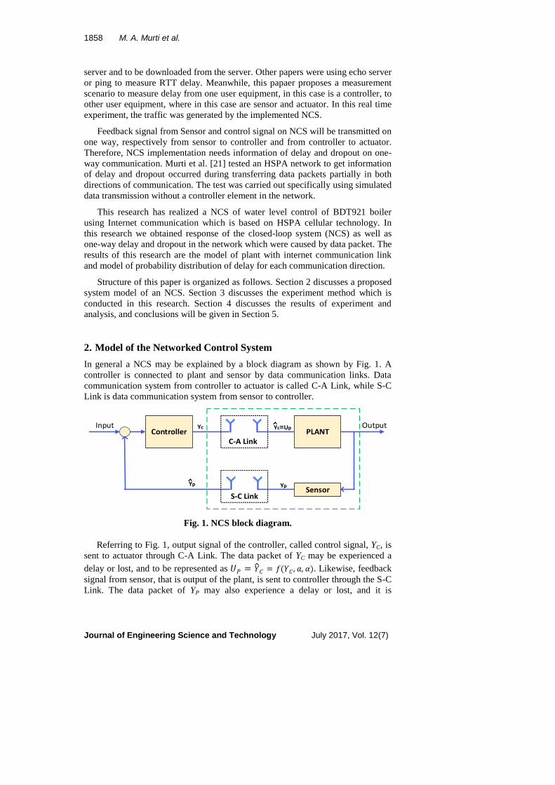
In general a NCS may be explained by a block diagram as shown by Fig. 1. A

controller is connected to plant and sensor by data communication links. Data

communication system from controller to actuator is called C-A Link, while S-C

Link is data communication system from sensor to controller.

PLANTInput Output

Controller

Sensor

C-A Link

S-C Link

Yc Yc=Up

Yp Yp

Fig. 1. NCS block diagram.

Referring to Fig. 1, output signal of the controller, called control signal, YC, is

sent to actuator through C-A Link. The data packet of YC may be experienced a

delay or lost, and to be represented as 𝑈𝑃 = �̂�𝐶 = 𝑓(𝑌𝐶 , 𝑎, 𝛼). Likewise, feedback

signal from sensor, that is output of the plant, is sent to controller through the S-C

Link. The data packet of YP may also experience a delay or lost, and it is



represented as 𝑈𝐶 = �̂�𝑃 = 𝑓(𝑌𝑃, 𝑏, 𝛽). By those background, the controller shown

in Fig. 1 is facing a plant system including the networks as shown in Fig. 2.

C-A Link PLANT S-C LinkYc = UCA Yc=Up Yp = UsC YSC = Yp

Fig. 2. Plant with data communication.

Referring to Fig. 2, consider the plant has a state-space model as:

𝑋𝑃(𝑘 + 1) = 𝐴𝑃𝑋𝑃(𝑘) + 𝐵𝑃𝑈𝑃(𝑘) (1)

𝑌𝑃(𝑘) = 𝐶𝑃𝑋𝑃(𝑘) + 𝐷𝑃𝑈𝑃(𝑘)

Meanwhile, C-A link has a state-space model as:

𝑋𝐶𝐴(𝑘 + 1) = 𝐴𝐶𝐴𝑋𝐶𝐴(𝑘) + 𝐵𝐶𝐴𝑈𝐶𝐴(𝑘) (2)

𝑌𝐶𝐴(𝑘) = 𝐶𝐶𝐴𝑋𝐶𝐴(𝑘)

and S-C link has a model of:

𝑋𝑆𝐶(𝑘 + 1) = 𝐴𝑆𝐶𝑋𝑆𝐶(𝑘) + 𝐵𝑆𝐶𝑈𝑆𝐶(𝑘) (3)

𝑌𝑆𝐶(𝑘) = 𝐶𝑆𝐶𝑋𝑆𝐶(𝑘)

In Fig. 2, the control signal U is sent to the plant through C-A link. YC will be

the input signal for block C-A or YC = U = UCA. Meanwhile output of the block

C-A, YCA, will be a control signal that is received by the plant, �̂� = 𝑌𝐶𝐴 = 𝑈𝑃.

Similarly, plant output of the feedback signal YP will be sent to the controller

through S-C link and become input signal for S-C link, YP = USC. The output

signal from S-C link is the estimated output of the plant, 𝑌�̂� = 𝑌𝑠𝑐.

Output of plant, YP (k), will experienced a delay of b seconds and if the delay

is greater than time allowed, the data will be dropped out. When the network is in

good condition and data from the plant is received in controller then β = 0.

Conversely, if the data network is in a bad condition due to some reasons and it

causes the dropout at S-C link, then β = 1. Similar to the data output from the

controller, YC(k) will be delivered to the plant through internet, and it will be

delayed for ɑ seconds. α = 0 when the data was arrived at the plant and α = 1 in

case of dropout at C-A link.

Using basic concept of delay and dropout given in [1], the received control

signal through C-A link can be written as:

)1()()1()( kUakUkU PCAP (4)

We assumed that )()( kUkX PCA and )()( kUkY PCA

Thus, state space model of C-A link can be written down as:

)1()1()()1( akUkXkX CACACA

(5)

)(.1)( kXkY CACA

Since )()( kUkX PCA , therefore Eq. (1) can be rewritten to be:



)()()1( kXBkXAkX CAPPPP (6)

)()(.)( kXDkXCkY CAPPPP

Similarly, the feedback signal from sensor to controller through S-A link can

be written as:

)1(ˆ)()1()(ˆ kYbkYkY PPP (7)

We assume that:

)(ˆ)( kYkX PSC and )()( kUkY SCP

and )()( kUkY SCP therefore Eq. (3) can be rewritten to be:

)1()1()1(.)1()(.)1( bkXDbkXCkXkX CAPPPSCSC

(8)

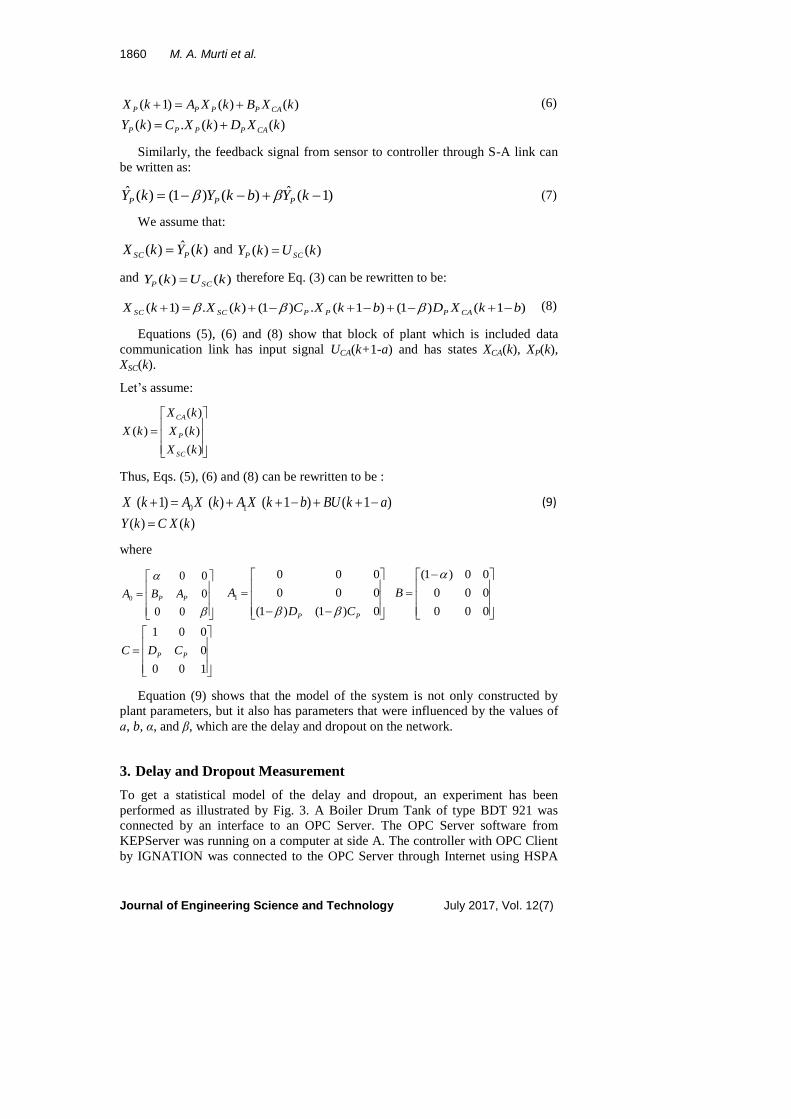
Equations (5), (6) and (8) show that block of plant which is included data

communication link has input signal UCA(k+1-a) and has states XCA(k), XP(k),

XSC(k).

Let’s assume:

)(

)(

)(

)(

kX

kX

kX

kX

SC

P

CA

Thus, Eqs. (5), (6) and (8) can be rewritten to be :

)1()1()()1( 10 akBUbkXAkXAkX

(9)

)()( kXCkY

where

00

0

00

0 PP ABA

0)1()1(

000

000

1

PP CD

A

000

000

00)1(

B

100

0

001

PP CDC

Equation (9) shows that the model of the system is not only constructed by

plant parameters, but it also has parameters that were influenced by the values of

ɑ, b, α, and β, which are the delay and dropout on the network.

3. Delay and Dropout Measurement

To get a statistical model of the delay and dropout, an experiment has been

performed as illustrated by Fig. 3. A Boiler Drum Tank of type BDT 921 was

connected by an interface to an OPC Server. The OPC Server software from

KEPServer was running on a computer at side A. The controller with OPC Client

by IGNATION was connected to the OPC Server through Internet using HSPA



modem. OPC Client was running on another computer at side B. The data

communication that takes place between computer A and B was recorded using

Wireshark on both sides.

The closed-loop system has implemented a PI controller to control water level

in the boiler tank. Using Ziegler-Nicholas method and manual adjustment as fine

tuning, then we have parameters of PI controller of Kp = 4 and Ki =0.181 with

input reference from 33 cm to 83 cm. The Experiments were conducted with two

scenarios to obtain data set of response system without Internet network, data set

of response system with Internet network, and data set of delay and dropout.

Fig. 3. Structure diagram of NCS experiment.

4. Result and Discussion

4.1. Control system without internet network

No Internet network in this case. Among elements of control system, they are

plant including sensor and actuator, and controller are connected directly. To get a

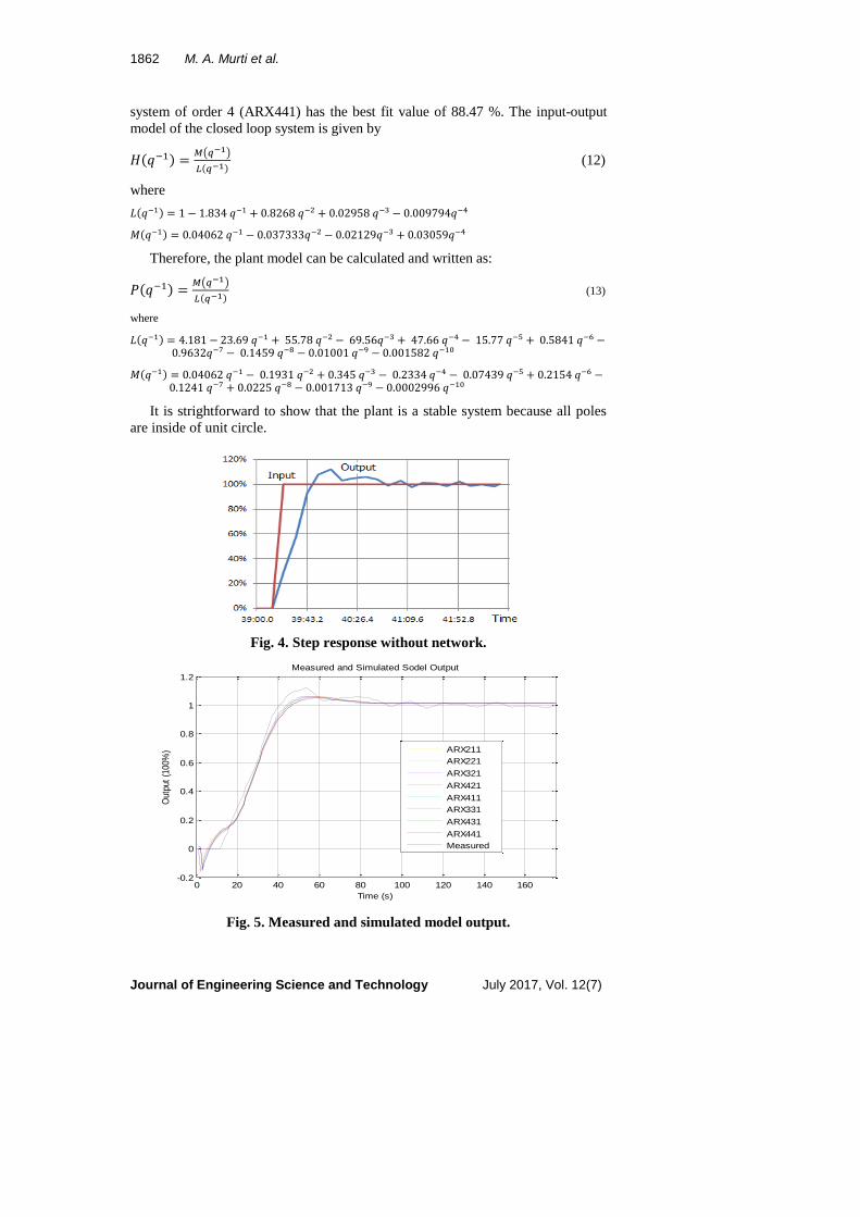
plant model, test has been carried out without Internet. Closed loop system was

implemented using PI Controller. The water level in the tank was changed

abruptly (step change) from 33 cm to 83 cm. The result has been obtained as

shown in Fig. 4. Figure 4 shows the step response of system in percentage.

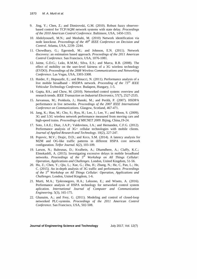
Using system identification tool of MATLAB, the model of the closed-loop system with ARX (Autoregressive Exogenous) structure has been obtained as shown in Fig. 5. ARX model is well suited for control design since this class of linear model is associated with a convex parameter estimation problem for both SISO and MIMO systems. A linear, discrete time, single input single output ARX model could be represented by the following equation:

𝐿(𝑞−1)𝑦(𝑡) = 𝑀(𝑞−1)𝑢(𝑡) + 𝜀(𝑡), 𝜀 ∈ 𝑁(0, 𝜎2) (10)

where L(q-1

) and M(q-1

) are polynomials of order n in the backwards shift operator q

-1 and ε(t) is white noise.

𝐿(𝑞−1) = 1 + 𝑎1𝑞−1 + 𝑎2𝑞−2 + ⋯ + 𝑎𝑛𝑞−𝑛 (11)

𝑀(𝑞−1) = 𝑏1𝑞−1 + 𝑏2𝑞−2 + ⋯ + 𝑏𝑛𝑞−𝑛

Figure 5 shows the simulated output of several ARX models. The index in

ARX model are indicating a number of poles, number of zeros, and number of

input samples that occur before the input affects the output. The best fits of each

estimated ARX model is shown by Table 1. The ARX model of closed loop



system of order 4 (ARX441) has the best fit value of 88.47 %. The input-output

model of the closed loop system is given by

𝐻(𝑞−1) =𝑀(𝑞−1)

𝐿(𝑞−1) (12)

where

𝐿(𝑞−1) = 1 − 1.834 𝑞−1 + 0.8268 𝑞−2 + 0.02958 𝑞−3 − 0.009794𝑞−4

𝑀(𝑞−1) = 0.04062 𝑞−1 − 0.037333𝑞−2 − 0.02129𝑞−3 + 0.03059𝑞−4

Therefore, the plant model can be calculated and written as:

𝑃(𝑞−1) =𝑀(𝑞−1)

𝐿(𝑞−1) (13)

where

𝐿(𝑞−1) = 4.181 − 23.69 𝑞−1 + 55.78 𝑞−2 − 69.56𝑞−3 + 47.66 𝑞−4 − 15.77 𝑞−5 + 0.5841 𝑞−6 − 0.9632𝑞−7 − 0.1459 𝑞−8 − 0.01001 𝑞−9 − 0.001582 𝑞−10

𝑀(𝑞−1) = 0.04062 𝑞−1 − 0.1931 𝑞−2 + 0.345 𝑞−3 − 0.2334 𝑞−4 − 0.07439 𝑞−5 + 0.2154 𝑞−6 −0.1241 𝑞−7 + 0.0225 𝑞−8 − 0.001713 𝑞−9 − 0.0002996 𝑞−10

It is strightforward to show that the plant is a stable system because all poles

are inside of unit circle.

Fig. 4. Step response without network.

Fig. 5. Measured and simulated model output.

0 20 40 60 80 100 120 140 160-0.2

0

0.2

0.4

0.6

0.8

1

1.2

Time (s)

Out

put

(100

%)

Measured and Simulated Sodel Output

ARX211

ARX221

ARX321

ARX421

ARX411

ARX331

ARX431

ARX441

Measured



Table 1. Best Fit of simulated model to measured output.

ARX Model Best Fits (%)

ARX441 88.47

ARX431 87.62

ARX331 87.3

ARX411 86.55

ARX421 86.55

ARX321 86.22

ARX221 85.72

ARX211 85.66

4.2. Control system with Internet network

This is an NCS, where connections of sensor to controller and controller to actuator

are used internet networks. In this case the plant under controlled is included sensor

and actuator as interfaces to the controller (See Figs. 1 and 2). To obtain set of data

of delay and dropout, an experiment is conducted upon an NCS as shown in Fig. 3.

Equation (12) with additional delay on network can be written as:

𝑌(𝑘) = 𝑁(𝜏)𝑀(𝑞−1)

𝐿(𝑞−1)𝑈(𝑘) (14)

where N(τ) consists of delay on C-A link (𝑎) and delay on S-C link (𝑏). In

condition of perfect model Eq. (14) should be equal to Eq. (9). But it is not

necessary since Eq. (9) is the proposed model which consists of plant and network

models as a system. The main issue is to obtain model of delay and dropout on

the network.

Figure 6 shows the response of system has 4.95% of overshoot, and settling

time was achieved in 23 seconds with steady-state error of 0.45%. Based on the

test results, we concluded that the system is stable and works normally. Therefore,

the captured data traffic over NCS with PI controller will be used to analyse the

delay and dropout on the network.

Fig. 6. Response of NCS with controller PI.

4.3. Data traffic record

During experiment of the closed-loop system with network, data traffic has been

recorded. Data packet size has average of 188 bytes with the largest size is 454

bytes for C-A link.



As for S-C link, it has average of 332 bytes with the largest packet size of 662

bytes. The delay and dropout caused by each packet can be seen in Fig. 7. The

delay varies with average delay of 0.1324 seconds for C-A Link and 0.3599

seconds for S-C link. Compare to [19] with 20 bytes of packet size, the average

RTT delay is 100ms, but 40% of packet bins have maximum RTT delay more

than 1 second.

Fig. 7. Data traffic record.

4.4. Dropout

Figure 8 shows dropout occurred several times for both directions. About 500

data packets of data have been sent with 15 dropouts in the direction of C-A link

and 3 dropouts in S-C link. Packet Loss can be calculated using the following

equation [21]:

𝑃𝑎𝑐𝑘𝑒𝑡 𝑙𝑜𝑠𝑠 = 𝐷𝑟𝑜𝑝 𝑜𝑢𝑡

𝑡𝑜𝑡𝑎𝑙 𝑝𝑎𝑐𝑘𝑒𝑡 (15)

(a). Delay and dropout in C-A link.

(b). Delay and dropout in S-C link.

Fig. 8. Delay and dropout.



Therefore, the resulted packet losses are 3% and 0.6% respectively for the

communication direction of C-A link and S-C link. If we consider both C-A link

and S-C link have upload at transmitter side and download at receiver, as shown

in Fig 3, then the result is lower than reported in [20], which is the packet loss rate

is 1.95% for uplink and 2.18% for downlink.

Packet Loss is very low because the data packet size is small and TTI

(Transmission Time Interval) is longer relatively to the data rate capacity of

Internet connection with HSPA technology. The experiment is conducted with

TTI = 1 second and the largest packet size is 662 bytes, and then data is with

highest rate as [21]:

bps296,51

8 x 662

TTI

sizepacket =BR (16)

Therefore, it requires Internet data rate less than 6 kbps. It is a significantly

low data rate in contrast to Internet capacity of HSPA technology which is up to

14 Mbps.

4.5. Probability distribution of delay

Statistical model of delay could be modelled by probability distribution [21].

Figure 9 shows an empirical distribution of delay in C-A link and S-C link.

Probability distribution of delay shown by Fig. 9 is close to Gaussian

distribution function. Gaussian distribution is one of common delay models. We

use basic Gaussian distribution as basic approach on delay modelling and

compare with experiment data. Therefore, using statistical data of mean and

standard deviation, we obtained Gausian like probability distribution shown by

Fig. 10. The mismatch between simulation and experiment is because there are

10% of data packets undergo high delays as shown in Fig. 9. Although the

number of events is very small, it increases the average value of delay. To avoid

the anomaly, the distribution can be recalculated by excluding 10% of the very

long time delay. We propose Gaussian distribution with corrected data and

Hidden Markov Model.

(a) C-A link. (b) S-C link.

Fig. 9. Probability distribution of delay.



(a) C-A Link. (b) S-C Link.

Fig. 10. Gaussian distribution of delay.

4.6. Corrected Gaussian distribution

If we assume a small amount of event with very long time delay that rarely appear

and can be ignored, it will obtain better results. As shown in Table 2, for the

direction of C-A link, in the case of which the delay greater than 0.2 seconds is

ignored, then average of delay is shifted from 0.132 seconds to 0.11 seconds.

Similarly, for the S-C link, the average of delay is changed from 0.36 seconds to

0.33 seconds. The distribution using average and standard deviation can be shown

in Fig. 11.

Table 2. Time delay statistical data.

C-A Link Delay (s) S-C Link Delay (s)

100% data 90% data 100% data 90% data

Mean 0.132 0.115 0.360 0.331

Min 0.041 0.040 0.123 0.123

Max 0.739 0.200 1.661 1.027

Standard Deviation 0.069 0.030 0.219 0.141


Fig. 11. Corrected Gaussian distribution of delay.

Using such modification, Correlation value and RMSE (Root Mean Square

Error) between the experimental data distribution and modified data distribution

are shown in Table 3.



As shown in Table 3, the modified Gaussian distribution models with

90% data packet has a correlation of 0.937 and 0.969 for the direction of

C-A link and S-C link respectively, while the RMSE values are 0.020 and 0.023

for the direction of C-A link and S-C link. It shows that removing a small

portion of data packet can represent a substantial delay distribution that

occurred in the experiment.

4.7. Hidden Markov Model (HMM)

The Markov model is a finite state model that describes the probability

distribution by a sequence of possibility. Figure 12 shows a Markov chain with

two states, S1 and S2. The probability of state changes from state j to state i is pji,

where pji < 0 and ∑ 𝑝𝑗𝑖 = 1𝑖 .

Fig. 12. Markov chain 2 states.

Sequential delay incident in Fig. 7 is a sequence of observations Oseq with n

data. Oseq is assumed as a hidden sequence of Sseq, corresponding to the following

equation [19]:

Oseq=O(1) , O(2) , …, O(k-1) , O(k) , O(k+1) ,..., O(n) (17)

Sseq=S(1) , S(2) , …, S(k-1) , S(k) , S(k+1) ,…, S(n)

where O(k) and S(k) are delay observation and corresponding state at sample time k.

State S1 represents condition with short delay, and S2 represents condition with

long delay, therefore the discrete state set is 𝑆(𝑘) ∈ 𝑆 = {𝑆1 , 𝑆2} with discrete

observation set is 𝑂(𝑘) ∈ 𝑂 = {𝑂1 , 𝑂2, … , 𝑂𝑛}. Let’s use mean values on Table 2

as threshold between short delay and long delay for each communication link.

Furthermore, the sequence of observations Oseq in Fig. 7 has sequence of states

Sseq as shown in Fig. 13 for C-A link and S-C link.

Using maximum likelihood estimation of the transition with data sequence

Oseq and Sseq, the transition matrices for C-A link and S-C link are:

𝑃𝑆𝐶 = [0.432 0.5680.496 0.504

]

𝑃𝐶𝐴 = [0.67 0.330.66 0.34

]

Transition matrix along with emission matrix can estimate the next state with

specific delay. Then let’s generate a number of delays by Hidden Markov Model

and investigate the probability distribution of generated delay as shown in Fig. 14.



(a) C-A link.

(b) S-C link.

Fig. 13. Sequence of states Sseq.


Fig. 14. Probability distribution of HMM.

As shown in Fig. 14 and Table 3, probability distribution of HMM has better

correlation compared with Gaussian distribution model, they are 0.988 for C-A

link and 0.995 S-C link. Furthermore, HMM also has better RMSE with 0.0199

for C-A link and 0.023 for S-C link.

Table 3. Correlation and RMSE of distribution models.

C-A Link S-C Link

Correlation RMSE Correlation RMSE

Gaussian 0.730 0.0334 0.867 0.0535

Corrected Gaussian 0.939 0.0199 0.969 0.0230

HMM 0,988 0,0056 0,995 0,0096

0

1

2

0 100 200 300 400 500

State C-A

0

1

2

0 100 200 300 400 500

State S-C



5. Conclusions

An investigation has been performed to obtain the statistical model of delay and

dropout on NCS with HSPA technology. This paper has discussed a model of plant

with a data communication network for both directions C-A link and S-C link in

the form of state space equations. In addition, an experiment has been carried out

to obtain an ARX model of plant in discrete transfer function. Dropouts occur

with 3% of packet loss rate resulting from NCS experiment conducted with data

packet size of 600 Bytes and TTI of 1 second. It also has been shown that

Gaussian distribution model can be used to represent delay probability

distribution with correlation of 0.93 and RMSE of 0.02. These results were

obtained when a small amount of data packet delay with high values is excluded

from the calculation. Hidden Markov Models with two states for low and high

delay may be used to estimate the delay. Probability distribution of delay by the

HMM delay estimator has correlation of 0.988 and 0.995, while RMSE values are

0.0056 and 0.0096 respectively for the C-A link and S-C link.

Actually the Gaussian delay model and the Hidden Markov delay model did

not considered dropout since the experiment shows there were very low of packet

loss rate. threfore, the delay models are only suitable for system with low packet

loss. It is an important for future work to find a model of delay and dropout on

both communication directions simultaneously as interactive model. This model

will be suitable for higher packet loss.

References

1. Murti, M.A.; Tjokronegoro, H.A.; Leksono, E.; and Wiseto, A. (2013).

Multi-delay multi-dropout model of M2M data network for networked

control system. Proceedings of the 19th

Asia Pacific Conference on

Communications. Bali, Indonesia, 509-513.

2. Luo, R.C.; Su, K.L.; Shen, S.H.; and Tsai, K.H. (2003). Networked

intelligent robots through the Internet: issues and opportunities. Journal:

Proceedings of the IEEE, 91(3), 371-382.

3. Ericsson. (2007). Basic concepts of HSPA. White paper 284 23-3087 Uen

Rev A. Ericsson. 1-20.

4. Bari, S.G.; Jadhav, K.P.; and Jagtap, V.P. (2013). High speed packet access.

International Journal of Engineering Trends and Technology, 4(8), 3422-3428.

5. Chamaken, A.; and Litz, L. (2010). Joint design of control and communication

in wireless networked control systems: a case study. Proceedings of the 2010

American Control Conference. Baltimore, USA, 1835-1840.

6. Li, Q.; Bugong, X.; and Shanbin, L. (2011). Modeling and analysis of

networked control system with random time delays and packet droputs.,

Proceeding of the 30th Chinese Control Conference. Yantai, China, 4527-4532.

7. Amelian, S.; Koofigar, H.R.; Vahdati, A.; and Vahdati, M. (2014). Digital

optimal control of multi-stand rolling mills with measurement and input delays.

Journal of Engineering Science and Technology (JESTEC), 9(2), 261-272.

8. Simon, S.; Gorgies, D.; Izak, M.; and Liu, S. (2010). Periodic observer

design for networked embedded control systems. Proceedings of the 2010

American Control Conference. Baltimore, USA, 4253-4258.



9. Jing, Y.; Chen, Z.; and Dimirovski, G.M. (2010). Robust fuzzy observer-

based control for TCP/AQM network systems with state delay. Proceedings

of the 2010 American Control Conference. Baltimore, USA, 1450-1355.

10. Abdolyousefi, M.N.; and Mesbahi, M. (2010) Network identification via

node knockout. Proceedings of the 49th

IEEE Conference on Decision and

Control. Atlanta, USA, 2239- 2244.

11. Chowdhary, G.; Egerstedt, M.; and Johnson, E.N. (2011). Network

discovery: an estimation based approach. Proceedings of the 2011 American

Control Conference. San Francisco, USA, 1076-1081.

12. Jaime, G.D.G.; Leão, R.M.M.; Silva, E.S.; and Marca, R.B. (2008). The

effect of mobility on the user-level fairness of a 3G wireless technology

(EVDO). Proceedings of the 2008 Wireless Communications and Networking

Conference. Las Vegas, USA, 3303-3308.

13. Haider, F.; Hepsaydir, E.; and Binucci, N. (2011). Performance analysis of a

live mobile broadband - HSDPA network. Proceeding of the 73rd

IEEE

Vehicular Technology Conference. Budapest, Hungary, 1-5.

14. Gupta, RA.; and Chow, M. (2010). Networked control system: overview and

research trends. IEEE Transaction on Industrial Electronics, 57(7), 2527-2535.

15. Jurvansuu, M.; Prokkola, J.; Hanski, M.; and Perälä, P. (2007). HSDPA

performance in live networks. Proceedings of the 2007 IEEE International

Conference on Communications. Glasgow, Scotland, 467-471.

16. Jang, K.; Han, M.; Cho, S.; Ryu, H.; Lee, J.; Lee, Y.; and Moon, S. (2009).

3G and 3.5G wireless network performance measured from moving cars and

high-speed trains. Proceedings of MICNET 2009. Bijing, China,19-24.

17. Soto, J.A.E.; Diaz, J.A.P.; Valdovinos, I.A.; and Hernandez, C.F.G. (2012).

Performance analysis of 3G+ cellular technologies with mobile clients.

Journal of Applied Research and Technology. 10(2), 227-247.

18. Popovic, M.V.; Drajic, D.D.; and Krco, S.M. (2014). A latency analysis for

M2M and OG-like traffic patterns in different HSPA core network

configuration. Telfor Journal. 6(2), 103-109.

19. Larson, N.; Baltrunas, D.; Kvalbein, A.; Dhamdhere, A.; Claffy, K.C.;

Elmokashfi, A. (2015). Investigating excessive delays in mobile broadband

networks. Proceedings of the 5th Workshop on All Things Cellular:

Operation, Applications and Challenges. London, United Kingdom, 51-56.

20. Hu, Z.; Chen, Y.; Qiu, L.; Xue, G.; Zhu, H.; Zhang, N.; He, C, Pan, L.; He,

C. (2015). An in-depth analysis of 3G traffic and performance. Proceedings

of the 5th Workshop on All Things Cellular: Operation, Applications and

Challenges. London, United Kingdom, 1-6.

21. Murti, M.A.; Tjokronegoro, H.A.; Leksono, E.; and Wiseto, A. (2016).

Performance analysis of HSPA technology for networked control system

aplication. International Journal of Computer and Communication

Engineering. 5(3), 165-175.

22. Ghanaim, A.; and Frey, G. (2011). Modeling and control of closed-loop

networked PLC-systems. Proceedings of the 2011 American Control

Conference. San Francisco, USA, 502-508.

statistic model of dynamic delay and dropout on …

Documents