STATIC AND DYNAMIC MEASUREMENTS OF RESERVOIRHETEROGENEITIES IN CARBONATE RESERVOIRS

Shameem Siddiqui, James Funk, and Aon KhameesSaudi Aramco Lab R&D Center, Dhahran, Saudi Arabia

AbstractHeterogeneity plays a critical role in determining the recovery from petroleum reservoirs.The determination of heterogeneities can be classified into static and dynamic techniques.CT and NMR techniques provide excellent means to determine the mobile fluid behaviorand the interactions of these mobile fluids with the confining surfaces of the pores.However, few studies have focused on the use of the interrelations of slice distributionsdetermined from these techniques.

In the present work, static heterogeneities were determined from distributionalmeasurements of core petrophysical properties including conventional whole core andplug data, profile permeametry measurements, CT number distributions and NMR T2

distributions. CT monitoring of displacement fronts during various stages of multi-phasecoreflood tests provided the dynamic measurements. Ambient condition corefloodingstudies on a three-plug composite core were conducted to show the dependence of fluiddisplacements on the microscopic heterogeneities existing in the core. The slice-by-slicedistributional data (porosity, permeability and saturation) in the horizontal direction wereused to visualize the position dependent variations. These were then compared withstandard heterogeneity parameters (Lorenz and Dykstra-Parsons) for both the discretesamples and the reservoir interval. Results showed that simple porosity-mappedheterogeneity indicators are unable to capture the variability in saturation distributions fortypical carbonate samples. However, even at the plug scale, expected deviations about amean value can be established based on the relative position of heterogeneities andstandard heterogeneity coefficients for the reservoir interval.

IntroductionComputerized Tomography (CT) is a non-destructive imaging technique that utilizes X-ray technology and mathematical reconstruction algorithms to view a cross-sectional sliceof an object. Since the early 80’s, the petroleum industry has been using CT-scanners asan effective tool for analyzing the reservoir cores. CT provides a non-destructive, non-invasive way of looking at cores and helps identify lithology, measure porosity anddetermine heterogeneity in three dimensions. The particular applications of CT as a rockdescription and core analysis tool include determination of fractures and heterogeneities,measurement of bulk density and porosity, visualization of mud invasion,characterization of lithology, evaluation of damage in unconsolidated cores and sectionalanalysis of cores. Apart from core characterization, CT used to visualize and quantifyfluid displacement in cores (both miscible and immiscible), to determine bulk density, todetermine residual oil saturation and trapped porosities, to visualize and quantify gravity

and viscous effects, etc. CT is mostly used for the determination of phase saturations inthe porous media. Detailed reviews of the application of CT in various corefloodexperiments can be found in the literature (Kantzas, 1990; Siddiqui, 1994).

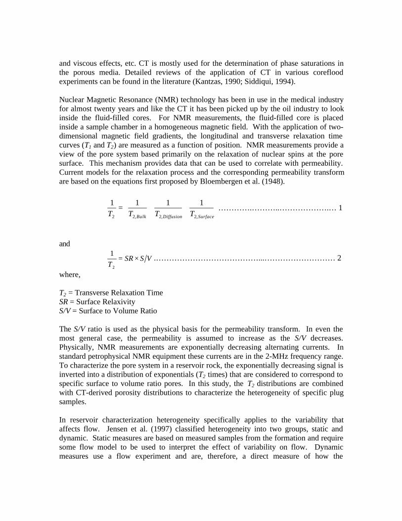
Nuclear Magnetic Resonance (NMR) technology has been in use in the medical industryfor almost twenty years and like the CT it has been picked up by the oil industry to lookinside the fluid-filled cores. For NMR measurements, the fluid-filled core is placedinside a sample chamber in a homogeneous magnetic field. With the application of two-dimensional magnetic field gradients, the longitudinal and transverse relaxation timecurves (T1 and T2) are measured as a function of position. NMR measurements provide aview of the pore system based primarily on the relaxation of nuclear spins at the poresurface. This mechanism provides data that can be used to correlate with permeability.Current models for the relaxation process and the corresponding permeability transformare based on the equations first proposed by Bloembergen et al. (1948).

++=

SurfaceDiffusionBulk TTTT ,2,2,22

1111………….………..……………….… 1

and

VSSRT

×=2

1.…………………………………...……………………… 2

where,

T2 = Transverse Relaxation TimeSR = Surface RelaxivityS/V = Surface to Volume Ratio

The S/V ratio is used as the physical basis for the permeability transform. In even themost general case, the permeability is assumed to increase as the S/V decreases.Physically, NMR measurements are exponentially decreasing alternating currents. Instandard petrophysical NMR equipment these currents are in the 2-MHz frequency range.To characterize the pore system in a reservoir rock, the exponentially decreasing signal isinverted into a distribution of exponentials (T2 times) that are considered to correspond tospecific surface to volume ratio pores. In this study, the T2 distributions are combinedwith CT-derived porosity distributions to characterize the heterogeneity of specific plugsamples.

In reservoir characterization heterogeneity specifically applies to the variability thataffects flow. Jensen et al. (1997) classified heterogeneity into two groups, static anddynamic. Static measures are based on measured samples from the formation and requiresome flow model to be used to interpret the effect of variability on flow. Dynamicmeasures use a flow experiment and are, therefore, a direct measure of how the

heterogeneity affects the flow. One of the commonly-used techniques for measuring thestatic heterogeneities is the Stile’s Plot, which gives the Lorenz Coefficient, Lc. Thetechnique involves ordering the product of permeability and the representative thickness(kh) in the descending order along with the corresponding porosity-representativethickness product (φh) for a well (or wells). The normalized cumulative values of kh,which also known as the fraction of total flow capacity (between 0 and 1) are then plottedagainst the normalized cumulative values of φh, which is also known as the fraction ofthe total volume (between 0 and 1). This plot is the so-called the Stile’s plot. The Lc iscalculated by comparing the area under the curve above a 45° line between (0,0 and 1,1)and 0.5. Lc can theoretically vary between 0 and 1, with 1 representing the highest degreeof heterogeneity. According to Jensen et al. (1997), Lc offers several advantages over theother more commonly-used heterogeneity indicator, the Dykstra-Parson’s coefficient.They include the fact that Lc can be calculated for any distribution (does not have to be anormal distribution), that Lc values do not depend on the best-fit procedures used and thatits evaluation includes porosity heterogeneity and variable thickness layers. Details ofthe procedures for calculating Lc and VDP can be found in the literature (Craig, 1971,Jensen et al., 1997).

The coefficient of variation, Cv is another lesser-known measure of heterogeneity. It is adimensionless measure of sample variability or dispersion and is given by,

)(

)(

xE

xVarCv = ………………………………………………...…………. 3

where, the numerator is the sample standard deviation and the denominator is the samplemean. Cv is being increasingly applied in geological and engineering studies as anassessment of permeability heterogeneity. For data from different populations, the meanand standard deviation often tend to change together such that Cv stays relativelyconstant. Any large changes in Cv between two samples indicate a dramatic difference inthe populations associated with those samples (Jensen et al., 1997).

ExperimentalThe cores used for this paper were selected from two vertical wells (designated as Well Aand Well B) from a Jurassic carbonate reservoir. Conventional core analysis work wasperformed on cores collected from the entire reservoir section using both 4" verticalwhole core samples and 1-1/2" horizontal plugs. For the whole cores, three different airpermeability measurements were made: one in the vertical direction (kvert), and two othersin the horizontal direction at 90 degrees to each other. The two horizontal permeabilitymeasurements are called kHMax and kH90, respectively in the paper, with the former beingthe maximum of the two permeability readings taken in any arbitrary direction.

A total of five 1-1/2" diameter carbonate plug samples from the two wells were selectedfor using in CT, NMR, Profile Permeametry and coreflooding studies. These are, plug

nos. 248 and 246, from Well A, and plug nos. 26, 157 and 100, from Well B. Thecapillary contact between two adjacent plugs was maintained by using circular filterpapers. All CT-scanning work was done using a Deltascan-100 scanner (120 KHz, 25mA, translate-rotate system). Coreflooding was conducted at room temperature and at2500-psi overburden pressure using a special coreflooding system consisting of Quizixpumps, a Temco FCH series coreholder and a Compumotor/AcuTrac table positioningsystem. Figure 1 shows a simplified schematic of the coreflooding system used.

The coreflooding test sequence for the composite plug from Well B included vacuum-saturation with brine, an oilflood (stopping for scanning after 0.2-PV, 10-PV and 20-PVof oil injected) and a waterflood (stopping for scanning after 1-PV, 10-PV and 20-PV ofwater injected). A constant flow rate of 5 cc/min was used during each stage ofcoreflooding, based on recommendations for stabilized flow. During CT-scanning, thecore was scanned at the same locations (0.5-cm inter-slice distance). An imagesubtraction technique involving voxel-by-voxel subtraction of the CT-data for the coreunder vacuum from the image data for the various stages of displacement was used toview and quantify the fluid movement. The image subtraction and most of the post-processing work was done using the VoxelCalc software on a SUN Ultra-60 workstation.

Two different methods were used for calculating porosity (φ) and porosity distributionsusing CT. The first of these methods, the standards method, involves scanning standardsof known bulk densities and plotting bulk density versus CT numbers. The slope and theintercept of the straight-line fit are then used to compute the bulk density (ρbulk) of theunknown samples. Once the bulk density is known, porosity at each volume element(voxel) can be calculated using Equation 4.

fluidmatrix

bulkmatrix

ρρρρ

φ−−

= …………………………………………….….……… 4

The other method involves taking the scan of the core under vacuum and when it is fullysaturated with brine, preferably containing a tracer such as sodium iodide. The equationused for calculating φ is given below.

airwater

drywet

CTCT

CTCT

−

−=φ …………………………………….…...……….…… 5

where, CTdry and CTwet are the mean CT numbers of the slice when the core is dry, andwhen it is saturated with brine containing a tracer, respectively. CTwater and CTair are themean CT numbers for the brine (containing tracer) and air, respectively. Details of bothtechniques can be found in the literature (Vinegar, 1986 and 1987; Withjack, 1988).

NMR measurements were made on 1.5" x 1.5" fluid saturated plugs in a Maran 2-MHzNMR instrument. Samples were wrapped in Teflon to minimize fluid loss during testing.The NMR signal was acquired using a CPMG (Carr-Purcell-Meiboom-Gill) pulsesequence acquiring 16,000 echoes with an inter-echo spacing of 0.10 ms. and apolarization time (delay time) of 7 s. Typically 150 scans were taken with a resultingsignal-to-noise ratio greater than 50. The echo trains were processed using a BDR(Butler, Dawson and Reed) algorithm on the phase-rotated signal. Regularization in theinversion equations was based on the signal-to-noise ratio for each individual sample.

Heterogeneity measurements at whole-core and plug scales were computed using theLorenz Coefficient (Lc) and the Dykstra-Parson's Coefficient (VDP). The pointpermeability data used for calculation of the Lorenz Coefficients for the plug sampleswere obtained using the NER Autolab Permeability System. A total of 8 measurementson the surface of the plugs (45°-apart from one another) were taken at each locationcorresponding to a particular 0.5-cm thick CT-slice. The NMR-based Lorenz coefficientswere calculated by ordering the surface-to-volume (S/V) ratio determined from the T2

distributions with the porosity distributions determined from CT scans. The method isbased on a simplification that the largest porosity intervals in the plug are most closelytied to the largest pore sizes.

Results and DiscussionFigures 2 and 3 are the CT-images of the slice porosities for the two carbonate plugs(#248 and #246) from Well A. The CT number data were used to generate bulk densitydata, which, in turn, were converted to porosities using the grain density data availablefrom routine core analysis. In these figures, in order to enhance the contrast between thevarious parts of the slices, the smallest possible porosity range is used (0.15 to 0.30). Thecolor legend is given in each figure at the top right-hand side. In these two figuresbrighter colors such as red and yellow represent a high porosity and darker colors such asblack and blue represent a low porosity. The overall porosity distribution (for all the CTslices) is given at the bottom of the figure. The porosity variation along a diagonal line(usually from lower left to upper right-hand corner of the slice) on any interesting slice ofeach plug is given at the upper left-hand corner. The predominance of brighter colors inFigure 2 indicates that plug #248 is more porous than plug #246. The large variation ofcolors in Figure 2 also indicates that plug #248 may be more heterogeneous than plug#246. Conventional core analysis data on plug nos. 248 and 246 gave porosities of 0.291and 0.228, respectively, with permeabilities of 961 md, and 648 md (at 2000 psig, roomtemperature), respectively.

Pore volume histograms for the two plugs together are shown in Figure 4. These arebased on the voxel-by-voxel porosity data for all the slices of an individual sampleplotted using 0.05% bin intervals. As shown in Figure 4, there is a slight differencebetween the porosity distribution and the PV-PHI distributions. Although CT-derivedporosity data can be calculated for each voxel, their arithmetic average does not representthe true porosity. Therefore the term PV-PHI (or pore volume-weighted porosity) is

used, which gives a better estimate of porosities from the CT-derived data. The porosityand the PV-PHI histograms cross over at the porosity bin size of 0.25. The increase in thepore volume distribution is due to the fact that more of the pore volume of the sample isdistributed in the portions of the sample with higher porosity. Discussions on PV-PHIcan be found in the literature (Funk et al. 1999).

Figure 5 shows the PV-PHI histograms for the individual plugs (#248 and #246). Thecorresponding NMR T2 distributions are shown in Figure 6. The T2 distributions aretypical of those seen in carbonates. In the absence of other data, the NMR distributionsgive a qualitative view of the plug sample heterogeneity but not a quantitative one. Thesamples are similar in that both show a large pore system (T2 distribution peak at 1 s)connected with a smaller pore system (T2 distribution peaks in the range of 90–300 ms).The distinction between the two pore systems is more pronounced in plug #248 than in#246. A third peak, seen at around 10 ms in the T2 distributions for plug #248 is mostlikely related to a small micropore system, the existence of which is confirmed by theSEM images.

Figure 7 shows three fresh-break SEM snapshots (A, B and C) and a back-scatteredimage (D) taken from one end of Plug #248. The snapshot A shows the same breakdownin pore body sizes seen in Figure 6 - a large subsystem with a diameter of 70-100 �m, asmall subsystem with 10 �m or smaller diameter and a very fine micro-crystallinesubsystem. The snapshot B shows the limestone and dolomite crystals and the snapshotC shows the very fine calcite crystals contributing to the smallest pore sizes. Thesnapshot D shows the back-scattered image for the area shown in the snapshot C and itgives the maximum projection of 1.6, with an aspect ratio of 1.4.

A sequence of static data, similar to the ones for Well A, is shown for the three-plug setfrom Well B. Figure 8 shows the porosities of individual slices arranged in the compositecore flood sequence (slices 1 through 7 representing Plug #26, 9 through 15 representingPlug #157, and 17 through 24 representing Plug #100, with slices 8 and 16 being thetransition slices). The porosity values obtained from conventional core analysis (at 2500psi and room temperature) for the three plugs in the above sequence are 0.281, 0.234 and0.243, respectively, with corresponding permeability values of 476, 338 and 471 md.The CT-derived porosity values match nicely with the conventional data and maintain theorder of porosities.

Figure 9 is the PV-PHI distribution for the individual samples based on CT data for thethree plugs (eliminating the transition slices). Figure 10 shows the corresponding NMRT2 distributions for the three plugs.

Dynamic two-phase data for the three-plug composite core from Well B are shown inFigures 11 and 12. Figure 11 represents the dynamic initial drainage data for 0.2-PV(pore volume) of injected oil and Figure 12 represents the dynamic drainage data at theend of a total of 20-PV of injected oil. In these two images, in order to enhance the

distribution of fluids inside the core, the matrix data were subtracted from the overallmatrix and fluid data on a voxel-by-voxel basis. Additionally the matrix-subtractedoilflood CT data were subtracted from the CT data corresponding to 100% brine (sodiumiodide doped) saturation. Details of the image subtraction technique used can be found inthe literature (Siddiqui et al., 1999).

In Figure 11 the effect of heterogeneity on fluid flow is highlighted by the non-uniformoil saturation front (before oil breakthrough) after injection of 0.2-PV of oil (shown asred). The vertical cross-section of the core shows slight override of the oil between slices11 and 13. More interestingly, both of these images show the presence of an unsweptregion (i.e. retention of water, shown as a blue diagonal line) between slices 1 and 8. Theporosity distribution slices for the first plug (#26), as seen in Figure 8, did not show anyunusually high- or low-porosity streaks. This heterogeneity in flow behavior, only seenduring dynamic conditions, could not be predicted from the CT-derived porositydistribution alone. However, the NMR T2 distributions may hold an important clue inthis matter.

Figure 12 shows the same core at irreducible water saturation (after 20-PV of oilinjection) with different plugs taking different amounts of oil. It also shows the existenceof the unswept region, even after the injection of 20-PV of oil.

The conventional data for Well A showed that the Lc depends not only on the orientationof the tested samples but also on the size. As shown in Figure 13, the Lc varied from 0.74for conventional horizontal plugs to 0.40 for whole core plugs, where the maximumhorizontal permeability was used. The Dykstra-Parson's coefficient for the horizontalplugs from Well A was calculated to be 0.91 (highly-heterogeneous). The Lc for all thehorizontal plugs from Well B was 0.75, very close to that for the horizontal plugs fromWell A.

On the plug scale, the various techniques for determining the Lc provided very similarresults. As expected, plug #248 from Well A was found to be more heterogeneous thanplug #246. As shown in Figure 14, the Lc for plug #248 determined using the CTporosity distributions and the NMR T2 distributions was 0.49, in close agreement withthat determined from the use of CT-derived porosity and profile permeability data, wherethe Lc was 0.50 . Results were in similar close agreement for plug #246 from Well A.The FZI-based Lc for the two plugs was the lowest (0.21), among all the Lc values. It wascalculated using CT-derived porosity data for the two plugs and the correspondingpermeability transform in the form k = a φn (applicable to the two plugs for 3<FZI<6).

Figure 15 shows that regardless of whether the porosity is determined by the CTstandards method (Equation 4) or by the CT saturation method (Equation 5), the averageporosity values are very close. The differences seen in plug #100 may be due toinsufficient saturation with water for this highly heterogeneous plug. The Cv values fromthe CT number data for the saturation method are generally higher than those for the

standards method. In general, the more heterogeneous plug (#100) also has the highestCv values for both methods.

What happens to Cv under dynamic conditions is generally a more complicated issue. Itappears that Cv for this case is a function of the local heterogeneities as well as the type offluids present in the core. Figure 16 shows the CT-derived saturation profiles inside the3-plug composite core during various stages of coreflooding. The assumption used forgenerating this plot is that uniform saturation existed throughout the core at the end ofwater circulation following saturation (called 100% water shown in blue at the top) and atthe end of 20-PV of oil (at irreducible water saturation of about 32%, shown in green atthe bottom). It also shows the two other saturation conditions representing 0.2-PV of oilinjected (shown in red and corresponding to Figure 11) and 20-PV of water injected(shown in brown, at residual oil saturation). The Cv values for the CT data used togenerate Figure 16 are shown in Figure 17. In general, the lowest values of Cv areobtained for the highest water saturation inside the core and the highest values of Cv areobtained for the lowest water saturation.

Conclusions1. The combination of CT and NMR data can reveal valuable information about

porosity and pore-size distributions that play an important role in fluid flowcharacterization and reservoir performance prediction. The two methods arecomplementary and provide a synergistic improvement in reservoircharacterization.

2. The combination of CT porosity distribution and NMR interpreted pore sizedistribution provides a convenient and accurate way to characterize theheterogeneity of individual core samples. This data can be critical for thecomparison of two-phase flow and other displacement processes in porous media.

3. Simple porosity-mapped heterogeneity indicators are unable to capture thevariability in saturation distributions for typical carbonate samples.

4. The coefficient of variation may hold important clues about the saturationconditions inside porous media in a multi-phase flow situation.

AcknowledgmentsThe authors wish to acknowledge the Saudi Arabian Ministry of Petroleum and MineralResources and the Saudi Arabian Oil Company (Saudi Aramco) for granting permissionto present and publish this paper. The authors also wish to acknowledge their colleaguesat the Petrophysics Unit and Sudhir Mehta at the Advanced Instruments Unit of SaudiAramco Lab R&D Center.

Nomenclaturea Coefficient used in the power-law

fit of the φ-k dataSR Surface Relaxivity

Cv Coefficient of Variation S/V Surface-to-Volume RatioE Expected Value of a Random

Variable xT1 Longitudinal Relaxation Time

FZI Flow Zone Indicator T2 Transverse Relaxation Timeh Reservoir or layer thickness Var Variance of a Random Variable xk Permeability VDP Dykstra-Parsons CoefficientLc Lorenz Coefficient φ Porosityn Exponent used in the power-law fit

of the φ-k dataρ Density

PV Pore Volume

ReferencesBloembergen, N., Purcell, E. M., and Pound, R. V.: "Relaxation Effects in Nuclear

Magnetic Absorption", Physics Review, 73, 1948, 679.Craig Jr., F. F.: The Reservoir Engineering Aspects of Waterflooding, SPE of A.I.M.E.,

Dallas, 1971, pp. 64-66.Funk J. J., Balobaid, Y. S., Al-Sardi, A. M. and Okasha, T. M.: Enhancement of

Reservoir Characteristics Modeling, Saudi Aramco Engineering Report No. 5684,Saudi Aramco, Dhahran, November, 1999.

Kantzas, A: "Investigation of Physical Properties of Porous Rocks and Fluid FlowPhenomena in Porous Media Using Computer Assisted Tomography," In Situ, Vol.14, No. 1, 1990, p. 77.

Jensen, J. L., Lake, L. L., Corbett, P. W. M. and Goggin, D. J.: Statistics for PetroleumEngineers and Geoscientists, Prentice Hall, Upper Saddle River, New Jersey, 1997,pp. 144-166.

Siddiqui, S.: Three Phase Dynamic Displacements in Porous Media, Ph.D. Dissertation,The Pennsylvania State University, University Park, PA, 1994.

Siddiqui, S., Khamees, A.A. and Velasco, V.B.: Three-Dimensional RelativePermeability and Dispersion Measurement using Computerized Tomography, SaudiAramco Engineering Report No. 5687, Saudi Aramco, Dhahran, December, 1999.

Vinegar, H. J.: "X-Ray CT and NMR Imaging of Rocks," Journal of PetroleumTechnology, March, 1986, p. 257.

Vinegar, H. J. and Wellington, S. L.: "Tomographic Imaging of Three-Phase FlowExperiments," Rev. Sci. Instrum., January, 1987, p. 96.

Wellington, S. L. and Vinegar, H. J.: "X-Ray Computerized Tomography," Journal ofPetroleum Technology, August, 1987, p. 885.

Withjack, E. M.: "Computed Tomography for Rock-Property Determination and Fluid-Flow Visualization," SPE paper 16951 presented at the 62nd Annual TechnicalConference and Exhibition of the SPE in Dallas, Texas, September 27-30, 1987.

Withjack, E. M.: "Computed Tomography for Rock-Property Determination and Fluid-Flow Visualization," SPE Formation Evaluation, December, 1988, p. 696.

Figure 1: Schematic of the coreflooding system and the CT-scanner.

Figure 2: CT-images of the slice porosities for plug#248 from Well A.

Figure 3: CT images of the slice porosities forplug #246 from Well A.

0.00

0.01

0.02

0.03

0.04

0.05

0.06

0.155 0.175 0.195 0.215 0.235 0.255 0.275 0.295 0.315 0.335 0.355 0.375 0.395 0.415 0.435

Porosity Bin Size (fraction)

No

rmalize

d F

req

uen

cy (

Po

rosit

y a

nd

PV

-PH

I)

PV-PHI (Normalized)

Porosity (Normalized)

Figure 4: Porosity and PV-PHI histograms forboth plugs (#248 and #246) from Well A.

0.00

0.01

0.02

0.03

0.04

0.05

0.06

0.07

0.08

0.09

0.10

0.11

0.15 0.20 0.25 0.30 0.35 0.40 0.45 0.50

Porosity (Bin Size)

No

rma

lize

d P

V-P

HI

Fre

qu

en

cy

PV-PHI (Normalized): 248

PV-PHI (Normalized): 246

248

246

Figure 5: PV-PHI histograms for each of theindividual plugs (#248 and #246) from Well A.

0.0

0.1

0.2

0.3

0.4

0.5

0.6

0.7

0.8

0.9

1.0

100 1000 10000 100000 1000000 10000000

T2 Time ( µµs)

No

rmalize

d S

ign

al

Inte

nsit

y

Sample 246

Sample 248

Figure 6: NMR T2 distributions for each of theindividual plugs (#248 and #246) from Well A.

Figure 7: SEM images of the freshly-brokensurfaces of plug #248 at different magnifications.

Figure 8: CT images of the slice porosities for thethree plugs (#26, #157 and #100) from Well B.

0.00

0.01

0.02

0.03

0.04

0.05

0.06

0.07

0.08

0.09

0.10

0.11

0.12

0.100 0.125 0.150 0.175 0.200 0.225 0.250 0.275 0.300 0.325 0.350 0.375 0.400

Porosity (Bin Size)

No

rma

lize

d P

V-P

HI

Fre

qu

en

cy

PV-PHI (Normalized): 26

PV-PHI (Normalized): 157

PV-PHI (Normalized): 100

157

100

26

Figure 9: PV-PHI histograms for each of theindividual plugs (#26, 157 and 100) from Well B.

0

1000

2000

3000

4000

5000

6000

7000

8000

9000

10000

100 1000 10000 100000 1000000 10000000

T2 Time ( µµs )

Sig

na

l In

ten

sit

y

Sample 157

Sample 100

Sample 26

Figure 10: NMR T2 distributions for each of theindividual plugs (#26, 157 and 100) from Well B.

Figure 11: Matrix-subtracted CT images of the 3-plug composite core from Well B after 0.2 PV ofoil is injected into the 100% water-saturated core.

Figure 12: Matrix-subtracted CT images of the 3-plug composite core from Well B after a total of 20PV of oil is injected into the 100% water-saturated

core.

0.0

0.1

0.2

0.3

0.4

0.5

0.6

0.7

0.8

0.9

1.0

0.0 0.1 0.2 0.3 0.4 0.5 0.6 0.7 0.8 0.9 1.0

Fraction of Total Flow Volume

Fra

ctio

n o

f Tota

l Flo

w C

apac

ity

Lc (Horiz. Plug) = (area ABCA) / (area ACDA) = 0.736Lc (Whole-Vert) = (area AB'CA) / (area ACDA) = 0.683Lc (Whole-H90) = (area AB''CA) / (area ACDA) = 0.442

Lc (Whole-Hmax) = (area AB'''CA) / (area ACDA) = 0.395

A

B

C

D

B'''

B'

B''

Figure 13: Stile’s plot for Well A showingvariations of Lc using various sources of

conventional core analysis data.

0.0

0.1

0.2

0.3

0.4

0.5

0.6

0.7

0.8

0.9

1.0

0.0 0.1 0.2 0.3 0.4 0.5 0.6 0.7 0.8 0.9 1.0

Fraction of Total Flow Volume

Fra

ctio

n o

f Tota

l Flo

w C

apac

ity

1 Lc(All Plugs from Well) = 0.756

2 Lc(Plug 248) = 0.4983 Lc(Plug 248)NMR = 0.485

4 Lc(Plug 248+246) = 0.458

5 Lc(Plug 246) = 0.3906 Lc(Plugs 246)NMR = 0.331

7 Lc(Plugs 246+248)FZI = 0.211

A

B

C

D

1

2

3

4

5

6

7

4

Figure 14: Stile’s plot for Well A showing thevariations of Lc values derived from individualplugs and their combinations using various CT

and NMR-based techniques.

0.22

0.23

0.24

0.25

0.26

0.27

0.28

0.29

0.0 0.1 0.2 0.3 0.4 0.5 0.6 0.7 0.8 0.9 1.0

Normalized Distance from Inlet End

Slice P

oro

sit

y (

fracti

on

)

0.0

0.1

0.2

0.3

0.4

0.5

0.6

0.7

0.8

0.9

1.0

Co

eff

icie

nt

of

Vari

ati

on

, C

v

Mean Porosity-Standards MethodMean Porosity-Saturation MethodCv-StandardsMethodCv - SaturationMethod

Plug #26 Plug #100Plug #157

Standards

Method

Sat.

Method

Figure 15: CT-derived average slice porosity values and Cv for the 3-plug composite core from Well B using the standardand the saturation methods.

0

10

20

30

40

50

60

70

80

90

100

0.0 0.1 0.2 0.3 0.4 0.5 0.6 0.7 0.8 0.9 1.0

Normalized Distance from Inlet End

Wate

r S

atu

rati

on

(%

)

100% Water

0.2 PV Oil Injected

20 PV Oil Injected

20 PV Water Injected

Figure 16: CT-derived saturation profiles for the 3-plug composite core from Well B during various stages of coreflooding.

0.10

0.12

0.14

0.16

0.18

0.20

0.22

0.24

0.26

0.28

0.30

0.0 0.1 0.2 0.3 0.4 0.5 0.6 0.7 0.8 0.9 1.0

Normalized Distance from Inlet End

Co

eff

icie

nt

of

Vari

ati

on

100% Water

0.2 PV Oil Injected

20 PV Oil Injected

20 PV Water Injected

Figure 17: CT-derived Cv values used for saturation calculation for the same conditions as shown in Figure 16.