Introduction to Supplemental.

This supplemental provides further supporting figures that could not be included in the manuscript. Table S1 lists the keywords used to query Twitter.

Figure S12 plots the silhouette scores associated with Figure 2, demonstrating that the number of clusters with the tightest clustering is two.

The section “Expert Curation of Tweets” describes how AM and NG curated tweets to validate labeling one cluster in Figure 2 as “MUPO” and the other “not MUPO”. This includes Tables S23 and S34. The statistical significance of this clustering is displayed In Table S4.

Figures S25 and S36 are the figures corresponding to Figure 5 for the 2013 and 2014 data collection periods.

The section “Calculation of Semantic Distance” describes our implementation of an ontology-based measurement of the semantic similarity of words. This includes Figures S47 and S58 and Table S5..

Table S1. Keywords used to query Twitter. A tweet was included in the signal category if the tweet contained at least one keyword. Division between “medical” and “street” names, made by NIDA, shown here for the sake of exposition. Not used in the acquisition or analysis of data.

Medical names Street names

morphine

methadone

codeine

hydrocodone

oxycodone

propoxyphene

fentanyl

tramadol

Roxanol

Duramorph

Empirin with

Codeine

Dope

Pain killers

Oxy

OC

Percs

Pancakes and

Syrup

Captain Cody

Demmies

Apache Chine

white

TNT

Oxy 80

Tango and Cash

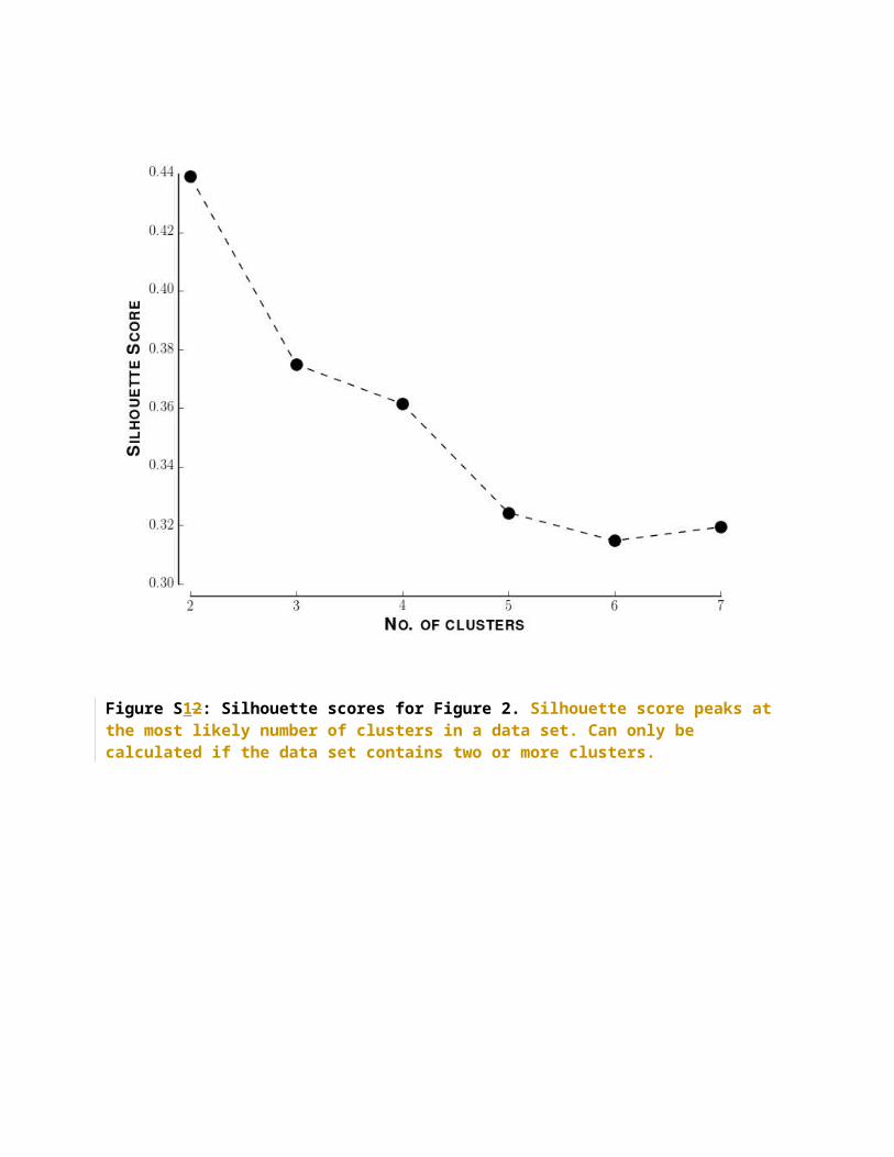
Figure S12: Silhouette scores for Figure 2. Silhouette score peaks at the most likely number of clusters in a data set. Can only be calculated if the data set contains two or more clusters.

Expert Curation of Tweets, Labeling of Semantic Clusters

Clustering tweets by semantic distance identifies groups of tweets with similar meaning.

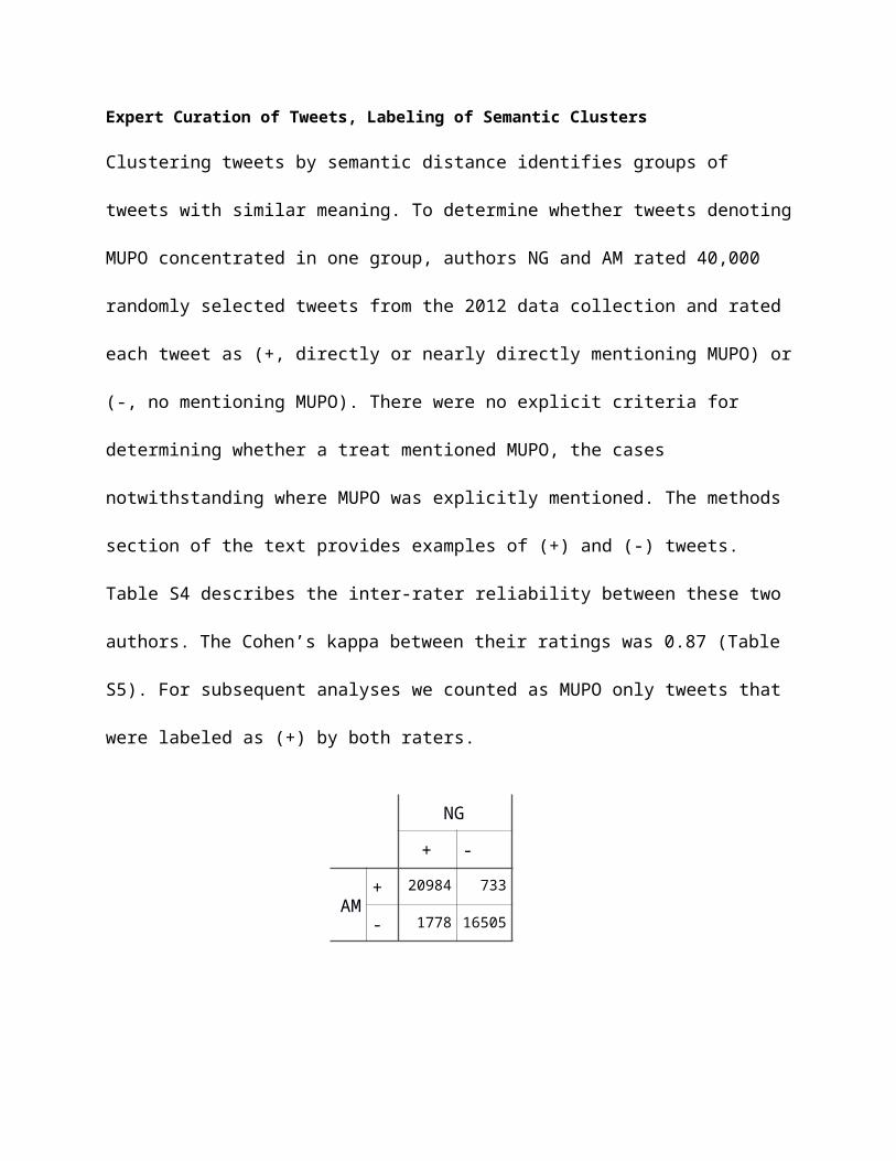
To determine whether tweets denoting MUPO concentrated in one group, authors NG

and AM rated 40,000 randomly selected tweets from the 2012 data collection and rated

each tweet as (+, directly or nearly directly mentioning MUPO) or (-, no mentioning

MUPO). There were no explicit criteria for determining whether a treat mentioned

MUPO, the cases notwithstanding where MUPO was explicitly mentioned. The methods

section of the text provides examples of (+) and (-) tweets. Table S4 describes the inter-

rater reliability between these two authors. The Cohen’s kappa between their ratings

was 0.87 (Table S5). For subsequent analyses we counted as MUPO only tweets that

were labeled as (+) by both raters.

Table S23: Inter-raterInterrater reliability between manual curators of 2012 tweets. (+) denotes "related to misuse of prescription pain medication (MUPO)". (-) denotes "not related to misuse of prescription pain medication (MUPO)".

Table S34: Calculation of Cohen's Kappa.

NG

+ -

AM+ 20984 733

- 1778 16505

Observed Agreement .9376Chance Agreement .5059Cohen's Kappa: (0.9376 - 0.5059)/(1-0.5059) = 0.87

Statistical Significance. We labeled as “MUPO” the tweet cluster enriched with MUPO

tweets. We assumed that the label of “MUPO” was valid if the “MUPO” cluster contained

significantly more MUPO tweets than did the other cluster. To determine enrichment we

calculated the ratio of the tweets labeled (+) to tweets labeled (-) for each cluster. We

established the statistical significance of this enrichment by randomly shuffling tweets

between the MUPO and non-MUPO clusters and then recalculating this enrichment

ratio in the MUPO cluster. If the enrichment ratio we observed in our data reflected an

underlying semantic difference between MUPO tweets and not MUPO tweets, rather

than chance, enrichment ratios generated by randomly shuffling tweets between

clusters should be significantly lower. We reshuffled 10,000 times. This approach,

sometimes termed bootstrapping, generated a probability density function. We directly

calculated the p-value of this enrichment as the ratio of the area under the curve in

Figure S5 greater than (to the right of) the 95th percentile to the total area under the

curve. We repeated this process for 2013 and 2014 (Table S46). To determine, for

2013 and 2014, which cluster predominantly referred to MUPO tweets we projected the

each year’s tweets alongside the 2012 tweets. We labeled the 2013 cluster as MUPO

whose centroid was closest to the cluster identified as MUPO in 2012. We repeated the

same procedure for 2014. This is the “nearest neighbors” approach.

Year p-value2012 0.01582013 0.03222014 0.021

Table S46. Statistical significance of cluster labeling. P-values estimated from empirical probability distribution function.

In summary, we wrote natural language processing software to cluster tweets by

meaning. We used manual curation by physicians to determine whether tweets

discussing MUPO were preferentially allocated to one cluster. We validated the

statistical significance of this differential allocation using bootstrapping.

Figure S25. Scatter plot of estimates of MUPO from NSDUH and Twitter for 2013. Title of each panel indicates NSDUH age range. Open circles are estimates for each state scaled as indicated in Methods. Solid line shows linear regression line.

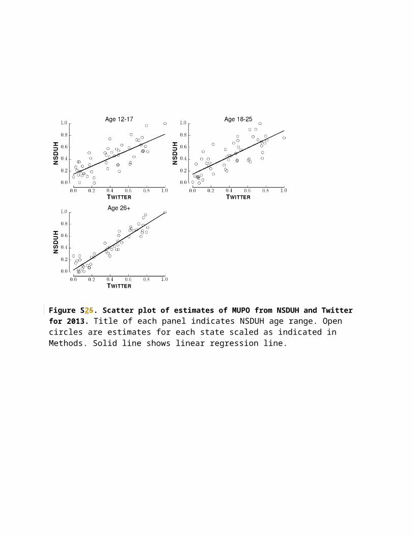
Figure S36. Scatter plot of estimates of MUPO from NSDUH and Twitter for 2014. Title of each panel indicates NSDUH age range. Open circles are estimates for each state scaled as indicated in Methods. Solid line shows linear regression line.

Calculation of semantic distance (SemD)

We used the semantic distance to partition the data stream from Twitter into

semantically distinct groups. Our implementation of SemD rests on the concept that the

more similar in meaning two words are the more synonyms they share. To make that

concept quantifiable, we exploit WordNet, a mind map of English that represents words

as clusters of synonyms. WordNet is a widely used map of semantic relations between

English words that has been extensively validated and is actively maintained. We

quantify the similarity in meaning between two words, as the distance between the

centers of mass of the two clusters of synonyms. This part of our calculation is identical

to other efforts to quantify semantic distance.

Our extension to the semantic distance involves the inclusion of context in the

calculation of the semantic distance. The context in which a word occurs helps specify

which meanings of that word are most germane. We include context by weighting the

combinations of meanings of each word with a kernel (vector), which we term the

Semantic Kernel. The ith entry of the semantic kernel represents the relative frequency

with which all synonyms of the ith meaning of a word occur in the text. For example, if a

list of words contains twice as many words pertaining to drugs as to aviation then, the

semantic kernel weights the meaning of high as in intoxicated with marijuana as twice

as likely as elevated in altitude.

Figure S47 shows the average fraction of words per tweet used in the calculation

of semantic distance. The left skew indicates that our approach did not capture all

words in calculating the semantic distance. Words that were not included corresponded

to words that were mis-spelled to the point of being unrecognizable or not in the lexicon

of WordNet, for example “xoxxxxo” or “bizsh*its”. Prior processing stages filtered out

emoticons. Efforts, such as PREDOSE [32], exist to extend the coverage of WordNet to

toxicologic and pharmacologic concepts, but are not yet fully integrated into WordNet

Figure S47. Distribution of fraction of words per tweet included in semantic distance calculation. Inset: Box plot of x-axis. Solid line indicates median, box indicates second and third quartile. Whisker indicates 90th percentile.

Having calculated the semantic distance between pairs of words, Figure S58 walks through the use of semantic distance to compare four tweets.

Figure S58. Calculation of semantic distance on four tweets. Lowercase d

with superscript hat denotes Jiang-Conrath similarity for each sense of the word.

Lowercase d with no superscript hat denotes semantic distance between tweets

designated by subscripts. No comparison with tweet (4), which contains no keywords

from Table S1.

Jiang-Conrath Similarity and WordNet

The Jiang-Conrath similarity between two meanings of a word is the distance to the nearest hypernym

both meanings share. Each word has many meanings, a property termed polysemy in linguistics.

WordNet represents meanings and so the Jiang-Conrath similarity, which uses WordNet as its input,

computes the similarity between meanings of words.

Text from social media contain words and so we designed our SemD to compare the similarity

between two words. While humans can often interpret which meaning is intended, there exists no way,

as of yet, for computers to do this. For our approach to be feasible for massive scale, automated

toxicosurveillance it is important to consider a computational approximation to context. We

approximated context by weighting the different possible meanings of a word by how many times the

synonyms of that meaning appeared in our entire corpus. Thus “high” was taken to be more likely to

mean “intoxicated with marijuana” than “elevated in altitude” because words related to marijuana were

mentioned more frequently than words related to aviation.

Construction of Semantic Similarity Matrix

We constructed a semantic similarity matrix to summarize the semantic similarity between tweets.

Albeit potentially confusing, we follow the machine learning convention of labeling any quantification of

the semantic relationship between two entities as “semantic similarity”, no matter whether the entities

are meanings, words, or phrases.

Table S5 shows an example to explain the construction of a semantic similarity matrix. We follow the

convention in machine learning of referring to entries in a matrix using row and column coordinates

rather than x- and y- coordinates. The rows are indexed by the letter i and the columns by the letter j.

The semantic similarity matrix presents measurements of distance, albeit an abstract one. (If the

distance measure is scaled to take on values between 0 and 1, then similarity = 1 – distance.) The matrix

must, accordingly, be symmetric across the diagonal. The distance between tweet i and tweet j is the

same as the distance between tweet j and tweet i. The entries on the diagonal must be 1 because each

entry is most similar to itself. In our example, Tweet 4 is most similar to Tweet 1 and Tweet 3 is least

similar to Tweet 1.

We constructed our semantic similarity matrix such that the rows and the columns of the matrix are the

individual tweets. The entry in the ith row and jth column of the matrix corresponds to the semantic

similarity between the ith and jth tweets. The semantic similarity of a tweet was the average SemD of

all combinations of words created by taking one word from the one tweet and another word from the

other tweet.

Tweet 1 Tweet 2 Tweet 3 Tweet 4

Tweet 1 1 0.3 0.1 0.8

Tweet 2 0.3 1 0.2 0.3

Tweet 3 0.1 0.2 1 0.4

Tweet 4 0.8 0.3 0.4 1

Table S5. Example semantic similarity matrix.