state estimation in power systems with combined ac … · state estimation in power systems with...

Ekaterina Telegina

State Estimation in Power Systems with

Combined AC and HVDC grids

Semester Thesis

PSL 1416

Institute:EEH – Power Systems Laboratory, ETH Zurich

Examiner:Prof. Dr. Goran Andersson, ETH Zurich

Supervisors:M.Sc. Roger Wiget, ETH Zurich

M.Sc. Philipp Fortenbacher, ETH Zurich

Zurich, July 2014

Abstract

The incorporation of Multiterminal High Voltage Direct Current (MTDC)grids in power transmission can be seen as a solution that will allow toincrease the transmission capacity of bulk transmission systems. An impor-tant example of such a system is European Network of Transmission SystemOperators for Electricity (ENTSO-e). Furthermore, it can enable an efficientintegration of the distantly located sources of renewable energy.

To ensure the secure operation of a combined power system, the Trans-mission System Operator (TSO) should be provided with the complete andaccurate information about the state of the system. However, due to suchfactors as measurement errors, communication noise and unavailability ofcertain measurements, the measurement data should be processed by a StateEstimation (SE) algorithm. This computational technique enables an effi-cient identification of the operating state of a system and is implementedin Energy Management Systems (EMS) of Alternating Current (AC) powersystems.

The objective of this thesis is to expand the existing SE technique forthe case of a combined power system with AC and MTDC grids by creatingan efficient and accurate SE algorithm on the base of the Weighted LeastSquares (WLS) algorithm for AC power systems.

i

Acknowledgement

First and foremost, I would like to express my gratitude to my supervisorsRoger Wiget and Philipp Fortenbacher for their constant support, encour-agement and insightful remarks. You really motivated me to work hard anddo my best.

I would also like to thank Professor Dr. Goran Andersson for giving methe opportunity to work on this interesting topic.

Special thanks to my family and friends for their continuous supportand understanding.

ii

Contents

List of Figures v

List of Tables vii

List of Abbreviations viii

List of Symbols ix

1 Introduction 1

1.1 Problem Definition . . . . . . . . . . . . . . . . . . . . . . . . 1

1.2 Literature Study . . . . . . . . . . . . . . . . . . . . . . . . . 1

1.3 Research Objectives . . . . . . . . . . . . . . . . . . . . . . . 2

1.4 Structure . . . . . . . . . . . . . . . . . . . . . . . . . . . . . 2

2 State Estimation of AC Power Systems 3

2.1 Functions of State Estimation . . . . . . . . . . . . . . . . . . 3

2.2 Weighted Least Squares State Estimation . . . . . . . . . . . 4

2.2.1 Weighted Least Squares Algorithm . . . . . . . . . . . 4

2.2.2 The Measurement Function . . . . . . . . . . . . . . . 7

2.2.3 The Measurement Jacobian . . . . . . . . . . . . . . . 8

2.3 Observability Analysis . . . . . . . . . . . . . . . . . . . . . . 8

2.4 Bad Data Analysis . . . . . . . . . . . . . . . . . . . . . . . . 9

3 State Estimation of Combined Power Systems 11

3.1 Existing Models . . . . . . . . . . . . . . . . . . . . . . . . . . 11

3.1.1 State Estimation Solution . . . . . . . . . . . . . . . . 11

3.1.2 Observability Analysis . . . . . . . . . . . . . . . . . . 14

3.2 Extended State Estimation Algorithm . . . . . . . . . . . . . 17

3.2.1 MTDC Power Systems Modelling . . . . . . . . . . . . 17

3.2.2 Weighted Least Squares Algorithm . . . . . . . . . . . 17

3.2.3 The Measurement Function . . . . . . . . . . . . . . . 19

3.2.4 The Measurement Jacobian . . . . . . . . . . . . . . . 21

iii



3.5 Implementation of the Algorithm in MATLAB . . . . . . . . 24

4 Case Study 28

4.1 Case Study Description . . . . . . . . . . . . . . . . . . . . . 28

4.2 Case Study. Results of the State Estimation . . . . . . . . . . 31



4.4.1 Bad Data in an AC measurement . . . . . . . . . . . . 35

4.4.2 Bad Data in a DC measurement . . . . . . . . . . . . 37

4.4.3 Measurement Data Set Corrupted by Noise . . . . . . 40

5 Discussion and Conclusion 42

Appendix A. Test Grid Parameters 43

Appendix B. Test Data Set 45

Appendix C. State Estimation Results 47

Appendix D. CD Contents 50

Bibliography 51

iv

List of Figures

2.1 Flowchart of the WLS Orthogonal Factorization SE . . . . . 6

3.1 Configuration of a generalized VSC-MTDC system a) sym-metric; b) asymmetric [7] . . . . . . . . . . . . . . . . . . . . 12

3.2 Equivalent circuit of the converter connecting the AC and DCgrid [7] . . . . . . . . . . . . . . . . . . . . . . . . . . . . . . . 13

3.3 Structure of the program implementing the extended SE al-gorithm in MATLAB . . . . . . . . . . . . . . . . . . . . . . . 24

4.1 Map of the combined power system with AC and MTDC gridsinvestigated in the case study . . . . . . . . . . . . . . . . . . 29

4.2 Case study results. AC voltage phase angles of the real andestimated state. AC 1: buses 1 - 16; AC 2: buses 17 - 32; AC3: buses 33 - 48. . . . . . . . . . . . . . . . . . . . . . . . . . 31

4.3 Case study results. AC voltage magnitudes of the real andestimated state. AC 1: buses 1 - 16; AC 2: buses 17 - 32; AC3: buses 33 - 48. . . . . . . . . . . . . . . . . . . . . . . . . . 32

4.4 Case study results. DC voltages of the real and estimated state. 33

4.5 Visualization of K-matrix (off-diagonal elements smaller than0.1 of the diagonal of the same row are deleted) . . . . . . . . 34

4.6 Case study results. AC voltage phase angles of the real,corrupted with a single AC bad measurement and correctedstate. AC 1: buses 1 - 16; AC 2: buses 17 - 32; AC 3: buses33 - 48. . . . . . . . . . . . . . . . . . . . . . . . . . . . . . . 35

4.7 Case study results. AC voltage magnitudes of the real, cor-rupted with a single AC bad measurement and correctedstate. AC 1: buses 1 - 16; AC 2: buses 17 - 32; AC 3:buses 33 - 48. . . . . . . . . . . . . . . . . . . . . . . . . . . . 36

4.8 Case study results. DC voltages of the real, corrupted with asingle AC bad measurement and corrected state. . . . . . . . 37

4.9 Case study results. AC voltage phase angles of the real,corrupted with a single DC bad measurement and correctedstate. AC 1: buses 1 - 16; AC 2: buses 17 - 32; AC 3: buses33 - 48. . . . . . . . . . . . . . . . . . . . . . . . . . . . . . . 38

4.10 Case study results. AC voltage magnitudes of the real, cor-rupted with a single DC bad measurement and correctedstate. AC 1: buses 1 - 16; AC 2: buses 17 - 32; AC 3:buses 33 - 48. . . . . . . . . . . . . . . . . . . . . . . . . . . . 39

v

4.11 Case study results. DC voltages magnitudes of the real, cor-rupted with a single DC bad measurement and corrected state. 40

4.12 The Normalized Root Mean Square Error of the SE algorithmfor different values of Gaussian noise standard deviation andthe extrapolation curve . . . . . . . . . . . . . . . . . . . . . 41

vi

List of Tables

4.1 The Normalized Root Mean Square Error of the SE algorithmfor different values of Gaussian noise standard deviation . . . 41

A.1 Susceptance of the shunt capacitors of the test grid, in p.u. [7,10] 43

A.2 Parameters of the AC branches of the test grid, all values inp.u. [7, 10] . . . . . . . . . . . . . . . . . . . . . . . . . . . . . 43

A.3 Resistance of the DC branches of the test grid, in p.u. [7] . . 44

A.4 Parameters of the model of active power losses in a converter [7] 44

B.1 Input data for PFC of AC 1 [10] . . . . . . . . . . . . . . . . 45



C.1 Real and estimated DC voltages of the test grid, in p.u. Dis-crepancy in values. . . . . . . . . . . . . . . . . . . . . . . . . 47

C.2 Real and estimated voltage angles and magnitudes of AC 1.Discrepancy in the values. . . . . . . . . . . . . . . . . . . . . 47



vii

List of Abbreviations

AC Alternating CurrentAC PS Alternating Current Power SystemCCI Correlation Coefficient of Injection MeasurementDC Direct CurrentEMS Energy Management SystemHVDC High Voltage Direct CurrentIEEE Institute of Electrical and Electronics EngineersMTDC Multiterminal (High Voltage) Direct CurrentNRMSE Normalized Root Mean Squared ErrorPFC Power Flow CalculationSCADA Supervisory Data Acquisition SystemSE State EstimationTSO Transmission System OperatorVSC Voltage Source ConvertersWLS SE Weighted Least Squares State Estimation

viii

List of Symbols

e measurement error vectorh(x) measurement function vectorH(x) measurement Jacobian matrixr residuals vectorR covariance matrixS residual sensitivity matrixΩ residual covariance matrixθ AC voltage angle vectorUDC DC voltage vectorV AC voltage magnitude vectorx state variables vectorx estimated state variables vectorz(x) measurement vector

Pinj AC active power injection vectorPflow AC active power flow vectorQinj AC reactive power injection vectorQflow AC reactive power flow vectorY AC bus admittance matrix

IDCinj DC current injection vectorIDCflow DC current flow vectorPDCinj DC power injection vectorPDCflow DC power flow vectorPloss vector of active power losses in convertersPC vector of active power injection from converters to AC gridsYDC DC bus admittance matrix

nbus number of buses in power systemnbusAC number of buses in alternating current power systemnbusDC number of buses in direct current power systemNAC number of interconnected AC gridsm number of measurementsmAC number of AC measurementsmDC number of DC measurements

ix

1

1 Introduction

1.1 Problem Definition

The complexity of modern power networks results in the challenging na-ture of the system control execution and normal operation maintenance. Tobe able to keep the power system in a normal secure state, the transmis-sion system operator (TSO) should be provided with sufficient and accurateinformation about the current operating state. This can be obtained byacquisition of measurements from different power system elements in Super-visory Control and Data Acquisition (SCADA). However, the measurementscan contain errors, be corrupted by noise or simply unavailable. Therefore,in order to correctly estimate the state of the system, the measurement datashould be processed by means of the State Estimation (SE) algorithm.

With the growing popularity of the Multiterminal High Voltage Di-rect Current (MTDC) grid concept as a reliable solution for interconnectionof several Alternating Current (AC) power systems and integration of thedistant renewable power sources, the problem of incorporation of MTDCsystems in the SE algorithm has become a question of vital importance. Toallow the identification of the operating state of a power system with com-bined AC and MTDC grids, the existing algorithm should be augmented andtested. This thesis addresses the problem of the expansion of the WeightedLeast Squares (WLS) SE algorithm on a combined AC and MTDC powersystem case.

1.2 Literature Study

The different aspects of the AC power system SE are explicitly describedin [1] and multiple other sources [2,3]. The specific AC Power System (PS)SE algorithm, used as a basis in this thesis, is presented in the lecturescript [4]. Augmentation of the SE technique for the combined AC andMTDC power systems is not sufficiently covered in the available sources.

There are quite a few works on incorporation of High Voltage DirectCurrent (HVDC) links (back-to-back or point-to-point) based on voltagesource converters (VSC) [5] or conventional current source converters [6]in SE algorithms. One possible concept of incorporation of MTDC powersystems in the SE algorithm is proposed in [7]. An approach to augmenta-tion of the observability analysis algorithm is described in [8]. The modelsintroduced in these two papers will be discussed in the following sections.The scarcity of the sources relevant to the topic justifies the demand on the

2 1 INTRODUCTION

further research regarding the subject.

1.3 Research Objectives

In this thesis, the power system SE technique is augmented on the case ofthe power system with combined AC and MTDC grids. This objective isfulfilled with the following steps:

• Study of the WLS PS SE algorithm and the existing models of itsexpansion on MTDC grids;

• Selection of the suitable approach to the modelling of a combinedpower system;

• Incorporation of the developed model in the SE algorithm;

• Implementation of the improved algorithm in MATLAB;

• Design of a combined power system for the case study and generationof a feasible test data set;

• Execution of the algorithm for the test power system;

• Analysis of the achieved results.

1.4 Structure

After this introduction the thesis has the following structure. The first partof Chapter 2 explains the methodology of WLS SE in AC power systems.In the subsequent sections of the chapter the observability analysis and baddata identification and correction tools for the AC case are discussed.

Chapter 3 describes the accomplished augmentation of the SE algorithmfor power systems with combined AC and MTDC grids and its implemen-tation in MATLAB.

In Chapter 4 the augmented algorithm is tested on a case study. Theresults of the corresponding computations are illustrated.

Chapter 5 discusses the results of the state estimation of a tested com-bined grid and provides the conclusions.

In Appendix A the test grid parameters are listed. Appendices B andC contain the test data set and the case study SE results correspondingly.In Appendix D the content of the enclosed CD is listed.

3

2 State Estimation of AC Power Systems

2.1 Functions of State Estimation

The state of the power system is defined by all complex voltages at all busesof the system. SE enables accurate and efficient monitoring of the currentstate of a power system based on which energy management system (EMS)functions can be incorporated. SE plays an important role in the controlof the real-time system operating conditions and contingency analysis. Itallows to derive an actual state of a power system from a noisy and/orincomplete measurement data set. The state estimators typically perform asuccessive implementation of the following functions [1]:

Topology processor gathers status data about the circuit breakers andswitches, and configures the one-line diagram of the system.

Observability analysis determines if an SE solution for the entire systemcan be obtained using the available set of measurements, identifies theunobservable branches, and the observable islands in the system if anyexist.

State estimation solution determines the optimal estimate for the sys-tem state, which is composed of complex bus voltages in the entirepower system, based on the network model and the gathered measure-ments from the system.

Bad data processing detects the existence of gross errors in the measure-ment set, identifies and eliminates bad measurements provided thatthere is enough redundancy in the measurement configuration.

Parameter and structural error processing estimates various networkparameters, such as transmission line model parameters, tap changingtransformer parameters, shunt capacitor or reactor parameters. It de-tects structural errors in the network configuration and identifies theerroneous breaker status provided that there is enough measurementredundancy.

This thesis addresses three of the stated functions, namely observabilityanalysis, SE solution and bad data processing. This choice is based ontheir important role in the estimation of an actual state of the system.Incorporation of two other processing tools in the developed algorithm canbe considered as a topic for the further research.

4 2 STATE ESTIMATION OF AC POWER SYSTEMS

2.2 Weighted Least Squares State Estimation

SE is based on processing of the measurements available in the power systemwith an appropriate network model. The modelling of the system compo-nents is described in [4]. It is assumed that the power system is in a steadyoperational state under balanced conditions. Therefore, a single phase pos-itive sequence equivalent circuit is applicable for its modelling.

The SE solution can be obtained by means of diverse techniques. Dif-ferent algorithms are compared in the article [9]. The traditional approachimplies the application of the Weighted Least Squares (WLS) iterative SEsolution algorithm. According to [1], this algorithm shows stable perfor-mance and can almost always successfully carry out the solution. However,the basic formulation of this algorithm requires matrix inversion which cancause convergence problems or even divergence. In order to circumvent theseshortcomings, different numerical techniques are used [4]. The formulationof the algorithm which is used in this thesis incorporates Orthogonal Fac-torization technique. This algorithm is briefly described in the followingsections.

2.2.1 Weighted Least Squares Algorithm

A SE algorithm should allow to derive a most probable state of the systemfrom the available measurement data set. In the WLS Algorithm the mea-surement errors are assumed to have a Gaussian (Normal) distribution withthe mean and the variance of the distribution as the parameters.

The state of an AC power system can be described with the systemvariables, namely voltage magnitudes and angles of the system nodes. Thestate variables build up a state vector:

x = [θ V ]T , (2.1)

where θ is the vector of the voltage angles of the system buses, and V isthe vector of the voltage magnitudes of the system buses. The state vectorcontains (2nbus − 1) unknown variables, where nbus designates the numberof the buses in the power system. One of the buses should be chosen asa reference bus, and therefore, its phase angle is set to an arbitrary value,such as 0. However, bus voltage angles are usually not measured directly.The state of the power system is typically estimated from a set of redundantmeasurements. This allows to mitigate the influence of measurement errorson the results of the SE. This data set z contains values such as activeand reactive power injections and power flows. As a part of SE algorithm,

2.2 Weighted Least Squares State Estimation 5

these values are derived as functions of the estimated state variables in themeasurement function h(x). The discrepancy between the measurementsdata set z and the measurement function h(x) is the measurement errorvector e:

z =

z1

z2

...

...

...zm

=

h1(x1, x2, ..., xn)h2(x1, x2, ..., xn)

...

...

...hm(x1, x2, ..., xn)

+

e1

e2

...

...

...em

= h(x) + e (2.2)

The WLS estimator minimizes the following objective function J(x):

J(x) =m∑i=1

(zi − hi(x))2/Rii = [z − h(x)]TR−1[z − h(x)], (2.3)

where m corresponds to the number of gathered measurements, zi and hiare the ith elements of the measurement vector z and measurement functionh. R in (2.3) represents the covariance of the measurement errors in the as-sumption that the measurement errors are independentR =diag

σ2

1, σ22, ..., σ

2n

.

In accordance to this, Rii is the variance of the ith measurement error. Asthe minimum, first order conditions should be met:

g(x) =∂J(x)

∂x= −HT (x) ·W · [z − h(x)] = 0, (2.4)

whereH(x) = ∂h(x)∂x is the measurement Jacobian and the matrixW = R−1

describes measurement accuracy. The solution of the WLS SE by means ofOrthogonal Factorization allows to avoid matrix decomposition. The WLSSE Orthogonal Factorization iteration procedure is described in [1] and hasthe sequence as in the flowchart depicted in Figure 2.1.


𝑥!

𝐻(𝑥!), ℎ(𝑥!)

𝑄!,𝑈 as QR

factorizarion of 𝐻! = 𝑊!/!𝐻

Δ𝑧! = 𝑄!!𝑊!/!Δ𝑧

solve 𝑈Δ𝑥 = Δ𝑧!

for Δ𝑥

𝑚𝑎𝑥!Δ𝑥𝑘! ≤ 𝜀?

NO

YES

END (𝑥! = 𝑥!)

START (𝑥!)

𝑘 = 𝑘 + 1

𝑥! = 𝑥! + Δ𝑥!

Figure 2.1: Flowchart of the WLS Orthogonal Factorization SE

In this flowchart xk is the estimate of the state vector at the kth itera-tion; H(xk),h(xk) are the measurement Jacobian and measurement func-tion calculated at the kth iteration; ε is the required accuracy of the SEsolution.

The initial guess of the state vector elements is typically the ”flat start”,when the values of voltage magnitudes are set to 1.0 p.u. and the values ofthe voltage angles are set to 0. The measurement function and measurementJacobian are calculated at each iteration, and using the Orthogonal Factor-ization the required change of the state variables is defined. This allows toobtain a new approximation of the state vector and run a new iteration ofthe SE algorithm. When the required accuracy of the solution is achieved,the iterations are stopped and the latest state vector approximation becomesan estimated state of the power system.

2.2 Weighted Least Squares State Estimation 7

2.2.2 The Measurement Function

The measurements obtained from the different parts of the power systemmost likely contain the line power flows, bus power injections and bus volt-age magnitudes. These measurements are expressed in terms of the statevariables in the measurement function:

h(θ,V ) =

Vmag

Pinj(θ,V )Pflow(θ,V )Qinj(θ,V )Qflow(θ,V )

(2.5)

where Vmag is the estimated voltage magnitude values; Pinj and Pflow arethe estimates of active power injections in the buses and active power flows inthe lines; Qinj andQflow are the estimates of reactive power power injectionsin the buses and reactive power flows in the lines. The expressions fordifferent measurement types are as following:

• Active and reactive power injection at bus i:

Pinji = Vi∑j∈Ni

Vj(Gijcosθij +Bijsinθij) (2.6)

Qinji = Vi∑j∈Ni

Vj(Gijsinθij −Bijcosθij) (2.7)

• Active and reactive power flow from bus i to bus j:

Pflowij = V 2i (gsi + gij)− ViVj(gijcosθij + bijsinθij) (2.8)

Qflowij = −V 2i (bsi + bij)− ViVj(gijsinθij − bijcosθij) (2.9)

where Vi, θi is the voltage magnitude and angle at the ith bus, θij = θi− θj ;Gij + jBij is the ijth element of the bus admittance matrix;gij + jbij is the admittance of the series branch connecting buses i and j;gsi + jbsi is the admittance of the shunt branch connected at bus i;Ni is the set of bus numbers that are directly connected to bus i.


2.2.3 The Measurement Jacobian

The measurement Jacobian H(θ,V ) has the following structure:

H(θ,V ) =

0∂Vmag

∂V

∂Pinj

∂θ∂Pinj

∂V

∂Pflow∂θ

∂Pflow∂V

∂Qinj

∂θ∂Qinj

∂V

∂Qflow∂θ

∂Qflow∂V

(2.10)

Each part of the measurement Jacobian (2.10) is a matrix consisting of thepartial derivatives of the measurement equations with respect to the statevariables. On the left side of the Jacobian matrix, the partial derivativeswith respect to the voltage angles are listed, on the right side there are thepartial derivatives with respect to the voltage magnitudes. For transmissionsystems, there is a strong coupling between active power and voltage angles,and between reactive power and voltage magnitudes. Under the assumptionthat the voltage angles are relatively small, the decoupled formulation of themeasurement Jacobian can be implemented:

H(θ,V ) =

0∂Vmag

∂V

∂Pinj

∂θ 0

∂Pflow∂θ 0

0∂Qinj

∂V

0 ∂Qflow∂V

(2.11)

2.3 Observability Analysis

Observability analysis determines which measurements should be executedin the power system in order to enable the power system SE. Different typesof measurements are described in the list below.

Critical measurement: elimination of that measurement from the mea-surement set results in an unobservable power system;

2.4 Bad Data Analysis 9

Redundant measurement: in case this measurement is eliminated fromthe measurement set, the power system is still observable;

Critical pair and critical k-tuple: two or k redundant measurements whosesimultaneous removal from the measurement set will make the powersystem unobservable;

Identification of the critical measurements can be accomplished by meansof the residual analysis. To conduct the residual analysis, the linearizedmeasurement equations should be considered:

∆z = H∆x+ e (2.12)

It is assumed that measurement errors are not correlated. The WLS esti-mator of the linearized state vector is given by:

∆x = G−1HTR−1∆z, (2.13)

where G = HTR−1H is called gain matrix. The estimated value of ∆z is:

∆z = H∆x = K∆z, (2.14)

where K = HG−1HTR−1. A large diagonal entry relative to the off-diagonal entries in the same row of the matrix K implies on a poor localredundancy. This feature enables the identification of the critical measure-ments in the data set. The measurement residuals and the measurementcovariance can be expressed as:

r = (I −K)e = Se (2.15)

Cov(r) = Ω = SW−1 (2.16)

where S is the residual sensitivity matrix, representing the sensitivity of themeasurement residual to measurement errors.

2.4 Bad Data Analysis

A SE algorithm should have a tool for identification and elimination ofthe measurements containing a large error (bad data). For the WLS SEmethod, detection and identification of the bad data can be performed bythe analysis of obtained residual values which are usually normalized bydividing their absolute values by the corresponding entries in the residualcovariance matrix Ω:

rNi =|ri|√Ωii

=|ri|√W−1

ii Sii

(2.17)


In the presence of a single bad data in a redundant measurement of the dataset, this bad measurement can be identified by finding the largest normalizedresidual. The faulty redundant measurement can be deleted from the dataset, and the SE algorithm can be run again to obtain a corrected state ofthe system. If all the residuals are smaller than a threshold that is chosenaccording to the measurement system accuracy, the conclusion is made thatthere is no bad data in redundant measurements of the data set. Detectionof the bad data in a critical measurement is not possible with this approach.

11

3 State Estimation of Combined Power Systems

In order to incorporate MTDC systems in the existing SE technique, thefollowing improvements should be done on the algorithm:

• an appropriate model of VSC converters and MTDC grid should beincorporated;

• the state variables of the MTDC power system should be defined andincluded in the state variables vector;

• the MTDC slack bus features should be defined;

• the measurements available in the MTDC grid should be identified;

• the measurement function should be augmented by the MTDC mea-surements;

• the measurement Jacobian should be augmented by the partial deriva-tives of the MTDC measurement function with respect to the MTDCstate variables;

• pseudomeasurements describing the coupling between AC and MTDCsystems should be included in the measurement function, their partialderivatives with respect to all state variables should be incorporatedin the measurement Jacobian;

• the adjustments of the observability analysis should be done, the tech-nique of critical MTDC measurements detection should be developed.

To develop an optimal approach to the resolution of the stated tasks, theearlier conducted relevant studies were analysed, and the short summary ofthe fulfilled analysis is presented in the next subsection.

3.1 Existing Models

In this section, several papers on HVDC state estimation problem are brieflyreviewed and discussed.

3.1.1 State Estimation Solution

In paper [7], a model of a VSC MTDC grid suitable for incorporation in WLSpower system SE algorithm is introduced. The generalized configuration ofa VSC-MTDC system, introduced in the paper, is illustrated in Figure 3.1.

12 3 STATE ESTIMATION OF COMBINED POWER SYSTEMS

Figure 3.1: Configuration of a generalized VSC-MTDC system a) symmetric;b) asymmetric [7]

From the AC side a converter is modelled as a controlled voltage source(Figure 3.2). The independent control of active and reactive power is per-formed by the use of corresponding equality constraints. One of the con-verters of MTDC system is set as controlling the DC voltage to compensatethe losses in the DC network. Besides that, the inequality constraints onthe operating area of VSC-MTDC are considered, namely the converter cur-rent constraint, converter DC voltage constraint and the DC cable currentconstraint. On the DC side, the converters are represented by a controllable

3.1 Existing Models 13

Figure 3.2: Equivalent circuit of the converter connecting the AC and DCgrid [7]

current source.

The measurement set proposed in [7] for AC/DC state estimation in-cludes traditional for WLS SE AC variables along with the DC voltage Udc,DC current injection, DC power injection, DC current flow, DC power flow;active and reactive power injections from converter Ps and Qs.

The state variables associated with the AC/DC interface are the sameas these in conventional AC state estimation formulations. Regarding theDC part, the DC voltage is chosen as the state variables, because once theseare known, the other variables such as current flow and power injections,can be calculated. The state vector of the whole DC system is Xdci =[Ufi θfi Uci θci Udci]

T for the ith converter.

The measurement equations for DC system and AC/DC interface arepresented in [7] as

Psi = Psi + ηps (3.1)

Qsi = Qsi + ηqs (3.2)

Udci = Udci + ηUdc(3.3)

Idci =

nd∑j=1

YdijUdci + ηIdc (3.4)

Pdci = Udci

nd∑j=1

YdijUdci + ηPdc(3.5)

Idcij = Ydij(Udci − Udcj) + ηIdcij (3.6)

Pdcij = UdciYdij(Udci − Udcj) + ηPdcij(3.7)


The equality constraints are introduced as pseudomeasurements:

0 = Pcfi − Psfi (3.8)

0 = Qcfi −Qsfi −Qfi (3.9)

x = [xac xdc]T , where xac contains (2nac − 2) unknown AC statevariables vector and xdc contains (5ndc − 2) unknown DC state variables.nac and ndc are the numbers of AC and DC buses. h = [hac hdc]T , wherehac is a mac × 1 AC measurement function vector, hdc is a mdc × 1 DCmeasurement function vector.

The Jacobian matrix of the combined grid is represented as

H(xac,xdc) =

[Hac−ac Hac−dc

Hdc−ac Hdc−dc

](3.10)

where Hac−ac is the Jacobian of traditional AC state estimation;Hac−dc = 0; Hdc−ac = ∂hdc

∂xac; Hdc−dc = ∂hdc

∂xdc.

The orders of the matrices Hac−ac,Hdc−ac and Hdc−dc aremac × (2nac − 2), mdc × (2nac − 2), mdc × 5ndc respectively.

In order to consider the operational limits of the converters, the esti-mated values are checked at the end of each iteration. If one variable is outof the limits, its value is fixed at the violated limit. In this situation, theJacobian matrix elements calculated with respect to the fixed state variableare considered equal to zero for the rest iterative process.

The proposed model is tested on the modified IEEE 14-bus system [10],with two offshore wind farms connected to buses 12 and 13. Simulationresults are stated to demonstrate the effectiveness of the proposed method.

3.1.2 Observability Analysis

The observability analysis technique for AC systems should be improvedto consider combined AC and MTDC grids. A concept of an improvedobservability analysis algorithm is proposed in [8].

Mathematical model of the VSC-AC system introduced in the paper isdivided into three parts: AC system, converters and DC network. A DCnetwork is described by the network equation

Id = GUd (3.11)

3.1 Existing Models 15

where Id and Ud are the vectors of direct current and direct voltage ofconverters at the terminals of DC network, and G is the node admittancematrix of DC network. The measurement vector of DC network is Zd =[Ud Id Pd]T . The state variable of each terminal is Udi of the converter.

The state of each converter is described by the variables vector X =[Usi Mi δi Udi]

T , where Usi represents voltage magnitude at the terminals ofthe coupling transformer of the converter, Mi is modulation ratio, δi is thelag angle between the terminals of the coupling transformer. If the activeand reactive power of the converter can be expressed as the function of Usi,the converter is defined as an effective converter. The measurement vectorof each converter is Zvsc = [Psi Qsi Mi δi]

T . The measurement equationsfor converter i are expressed by the variables as follows.

Pmsi = (UsiUci/Xli)sinδi =

µ√2Xli

UsiMiUdisinδi = f(Usi,Mi, δi, Udi) (3.12)

Qmsi =

Usi

Xli(Usi − Ucicosδi) =

Usi

Xli(Usi −

µMiUdi√2

cosδi) = f(Usi,Mi, δi, Udi)

(3.13)Mm

i = Mi (3.14)

δmi = δi (3.15)

The interaction between DC network and converters can be analysedin two aspects:

1. The DC network is observable. If the DC network is observable, Udi

and Pdi of every terminal are solvable. Therefore, Udi and Pdi of con-verters connected by the observable DC network can be regarded asequivalent measurements for the observability of converters in VSC-HVDC system.

2. The converter in VSC-HVDC system is observable. If the converteri in VSC-HVDC system is observable, Udi and Psi can be solved atthe converter side. Therefore, Udi and Psi of the observable convertercan be treated as equivalent measurements of DC network for theobservability of DC network.

The authors of the paper derived an algotithm for VSC-AC systemobservability analysis based on the following rules:

1. DC network rule: if the number of independent relation equationsabout DC voltage according to the available measurements is largerthan N which is the number of converters in VSC-HVDC, the DCnetwork is observable.


2. Converter rule: if the number of measurements inZvsc−oi = [Usi Psi Qsi Mi δi Udi]

T is larger than 4, the associatedconverter is observable. The number of measurements available shouldnot be less than the number of variables in the measurement equations.

3. Effective converter rule: if the number of measurements in Zvsc−ei =[Psi Qsi Mi δi Udi]

T is larger than 3, the associated converter is aneffective converter.

The proposed algorithm consists of the following steps:

1. Test the observability of DC network using the DC network rule. Ifthe DC network is observable, Psi and Udi are provided to convertersconnected by this DC network as equivalent measurements.

2. Identify the effective converters in the VSC-HVDC system one by one.Form the correlation coefficient of injection measurement (CCI) ofboundary buses. CCI equals to the number of converters subtractingthe number of effective converters connected to the boundary buses.

3. Add the injection measurements on boundary buses with CCI=0 asequivalent measurements to AC system. Perform observability analy-sis of AC system and identify all islands of AC system. If the islandhas at least one AC voltage magnitude measurement, this island isobservable.

4. Find out all converters in observable islands and update the corre-sponding Zvsc−oi with Usi. If the boundary buses in observable islandshave injection measurements, the corresponding Zvsc−oi will also beupdated with Psi and Qsi.

5. Test the observability of converters in VSC-HVDC system one by onewith Converter rule. If the converter is observable, add an equivalentAC voltage magnitude measurement to the corresponding island wherethe observable converter locates.

6. If any island in AC system is extended in step 3, return to step 1. Ifnot, stop and output the observable islands and observable constraints.

3.2 Extended State Estimation Algorithm 17

3.2 Extended State Estimation Algorithm

3.2.1 MTDC Power Systems Modelling

The first step of the incorporation of an MTDC PS into SE technique de-scribed in Chapter 2 is modelling of its elements, namely MTDC grid andVSC converters. In this thesis, an approach to modelling of the VSC con-verter as a voltage source on the AC side and a current source on the DCside proposed in [7] is adopted (Figure 3.2). On the AC side, the equivalentcircuit of a converter has three buses, two branches and one shunt. Thesebuses represent a point of connection of a coupling transformer to the ACgrid, a point of an AC filter connection and an AC side converter bus. Thebranches of the model have impedances of a coupling transformer and aphase reactor. This equivalent AC circuit can be shortly named AC/DCinterface. The shunt capacitor coincides with an AC filter. Unlike it isproposed in [7], the AC/DC interface measurements are considered as ACmeasurements, since they are taken on the AC side and represent AC volt-ages, power injections and power flows. The state variables of the busescorresponding to the AC/DC interface, namely AC voltage angles and mag-nitudes, are attributed to the AC state vector.

The MTDC grid is modelled by a bus admittance matrix, built up inthe same way as for an AC grid. One of the converters is set to control DCvoltage. The corresponding bus of the MTDC grid is chosen as slack. Thecoupling of the AC and MTDC grids is accomplished by maintenance of theactive power balance constraint of each converter. Active power losses in aconverter are modelled the same way as proposed in [7].

In contrast to [7], converter controllers and operating area constraintsare not incorporated in the algorithm developed in this thesis. The reasonof this decision lies in the main objective of this work to develop a highlyefficient SE algorithm whose performance can be clearly assessed at thecurrent research stage. Though it can be supplemented by diverse modellingcomplexities in case any further research follows.

3.2.2 Weighted Least Squares Algorithm

In this thesis, WLS Algorithm, described in Chapter 2 as a technique of SEof AC power systems, is applied for state estimation of combined AC andMTDC power systems. In order to incorporate the models of the MTDCgrid, the state vector x should be augmented with MTDC state variables.The state of the buses of MTDC is characterized by DC voltages. Provided


with DC voltages and MTDC grid topology and parameters, one can calcu-late other important values, such as DC power injections and power flows,and DC currents. This is implemented in the augmented measurement func-tion h(x). Besides that, the state variables of the AC/DC interface, namelyAC voltage magnitudes and angles of each converter and AC filter connec-tion buses, should be included as variables in the state vector.

The state vector of such a combined system is defined as:

x = [θ V UDC]T , (3.16)

where UDC defines voltage values in the buses of the MTDC grid (DCvoltages).

The state vector contains∑NAC

j=1 (2nbusACj − 1) + (nbusDC− 1) unknownvariables. NAC designates the number of the AC systems in a combinedsystem; nbusACj and nbusDC are the numbers of the buses in the jth ACsystem and in the MTDC grid correspondingly. The number of the slackbuses in a combined system depends on the number of AC power systemsinterconnected by the MTDC grid. One of the buses of the MTDC gridshould be chosen as a slack bus, and the value of its DC voltage should befixed. Each AC system involved into the interconnection should have its ownslack bus with a fixed value of the voltage angle. In the developed algorithmthe slack bus of each AC system is set to the point of connection of thedecoupling transformer to the AC grid. This means that the active powerbalance of each AC system should be attained at this point of the AC/DCinterface. In addition to this, AC voltage angles of each AC system arecalculated in reference to the angle at this point of connection. Typically,voltage angles of the slack buses are set to zero.

In case the MTDC grid is not connecting several AC systems but is justconnected to one AC system, only two slack buses should be defined: oneAC and one DC. Therefore, the state vector contains 2nbusAC + nbusDC − 2state variables.

The initial guess corresponds to the ”flat start” which for a combinedsystem means that along with AC voltage magnitudes set to one and anglesset zero, all the DC voltages are set to one.

The measurement vector of a PS with combined AC and MTDC gridsconsists of three parts: AC measurements; DC measurements and activepower balance pseudomeasurements. The measurement vector has the fol-lowing structure:

Z = [ZAC ZDC Zbal]T , (3.17)

where ZAC is built up from the measurements available on the AC side


including the measurements obtained from the AC/DC interface buses andbranches of the converters. These measurements are voltage magnitudes,active and reactive power injections and flows. However, some of the mea-surements can not be obtained from the technical standpoint, for example,the power injections directly from/to the converter. Along with this, someother possible measurements can be unavailable or economically not feasibleto conduct. For example, in absence of the active power flow measurements,the AC measurement vector can have a following structure:

ZAC = [Vmag Pinj Qinj Qflow]T . (3.18)

The DC measurement vector ZDC is comprised by DC voltages, DC currentinjections IDCinj, active power injections PDCinj, DC current flows IDCflow,and active flows PDCflow :

ZDC = [UDC IDCinj PDCinj IDCflow PDCflow]T . (3.19)

The third part of the measurement vector corresponds to the activepower balance pseudomeasurements. This part is needed in order to createthe coupling between AC and MTDC systems. The equations describingthe power balance in a converter are adopted from [7] and also reflect theactive power losses.

Zbal = [PC + PDC + Ploss] = 0, (3.20)

where PC is the vector of active power injections from the converters to theAC grid, PDC is the vector of power injections from the converters to theDC grid, and Ploss is the vector of active power losses in the converters.

The measurement vector is compared to the measurement function cal-culated based on the values of the state variables. The discrepancy betweenthe corresponding elements of these two vectors is calculated in the vector ofmeasurement errors. The WLS SE Algorithm provides the iterative solutionof the minimization problem defined by (2.3). The sequence of the steps ofthe algorithm corresponds to the one illustrated in Figure 2.1.

3.2.3 The Measurement Function

As stated above, all the measured values can be expressed in the terms ofthe state variables. The corresponding equations comprise the measurementfunction. The structure of the measurement function corresponds to the oneof the measurement vector: h = [hAC hDC hbal]

T .

The elements of the AC part of the measurement function are the valuesmeasured on the AC side and expressed in the AC state variables:


hAC = [Vmag Pinj Qinj Qflow]T . More details on this function were givenin Sec. 2.2.2.

In the DC part of the function, the DC values are calculated in termsof the DC state variables, namely DC voltages:hDC = [UDC IDCinj PDCinj IDCflow PDCflow]T .

hDC(UDC) =

UDC1

UDC2...

UDCnbusDC∑nbusDCj=1 YDC1jUDCj∑nbusDCj=1 YDC2jUDCj

...∑nbusDCj=1 YDCnbusDCjUDCj

UDC1∑nbusDC

j=1 YDC1jUDCj

UDC2∑nbusDC

j=1 YDC2jUDCj

...UDCnbusDC

∑nbusDCj=1 YDCnbusDCjUDCj

YDCij(UDCi − UDCj)YDCij(UDCi − UDCj)

...YDCij(UDCi − UDCj)

UDCiYDCij(UDCi − UDCj)UDCiYDCij(UDCi − UDCj)

...UDCiYDCij(UDCi − UDCj)

(3.21)

The third part of the measurement function corresponds to the balanceequations and has the following elements:

balk = PCk + PDCk + Plossk (3.22)

where k is the number of the AC system from 1 to NAC, balk is the estimatedactive power balance in the kth converter, PCk is the estimates of the activeand reactive power injections from the kth converter to the kth AC grid,


PDCk is the estimated active power injections from the kth converter to theMTDC grid Plossk is the active power losses estimation in the kth converterdefined by

Plossk = a+ bICk + cI2Ck, (3.23)

where ICk is the estimated current injection from the kth converter to the

AC grid calculated as ICk =

√P 2Ck+Q2

CkUCk

.

3.2.4 The Measurement Jacobian

The measurement Jacobian of a combined power system has the followingstructure:

H(xAC,xDC) =

HAC−AC HAC−DC

HDC−AC HDC−DC

Hbal−AC Hbal−DC

=

HAC−AC 00 HDC−DC

Hbal−AC Hbal−DC

(3.24)

Since the AC measurements are the functions of the AC state variables,and the DC measurements are the functions of the DC state variables, thecomponents HAC−DC and HDC−AC are zero matrices which have mAC ×(nbusDC − 1) and mDC × (2nbusAC −NAC) sizes correspondingly.

The matrix HAC−AC is the measurement Jacobian of the AC grids,its dimensions are mAC × (2nbusDC − NAC). The structure of this matrixcorresponds to (2.10) or (2.11) in case of the decoupled formulation of theAC measurement Jacobian is implemented.

The DC measurement Jacobian,HDC−DC, has the sizemDC×(nbusDC−1). This matrix has a structure as stated below:

HDC−DC(UDC) =

∂UDC∂UDC

∂IDCinj

∂UDC

∂PDCinj

∂UDC

∂IDCflow∂UDC

∂PDCflow∂UDC

(3.25)

The elements of the DC measurement Jacobian can be calculated using theequations below:


• Elements corresponding to the DC voltage measurements:

∂UDCi

∂UDCi= 1 (3.26)

∂UDCi

∂UDCj= 0 (3.27)

• Elements corresponding to the DC current injection measurements:

∂IDCinji

∂UDCi= YDCii (3.28)

∂IDCinji

∂UDCj= YDCij (3.29)

• Elements corresponding to the DC power injection measurements:

∂PDCinji

∂UDCi= YDCiiUDCi +

nbusDC∑j=1

YDCijUDCj (3.30)

∂PDCinji

∂UDCj= YDCijUDCi (3.31)

• Elements corresponding to the DC current flow measurements:

∂IDCflowij

∂UDCi= YDCij (3.32)

∂IDCflowij

∂UDCj= −YDCij (3.33)

• Elements corresponding to the DC power flow measurements:

∂PDCflowij

∂UDCi= YDCij(2UDCi − UDCj) (3.34)

∂PDCflowij

∂UDCj= −YDCijUDCi (3.35)

The parts of the measurement Jacobian of a combined power system that al-lows coupling between AC and MTDC grids are the partial derivatives of thebalance equations with respect to the state variables. The matrix Hbal−AC

has the size NAC × (2nbusAC −NAC). In case of a decoupled formulation ofthe Jacobian it has the following elements:

∂balk∂θi

=∂PCk

∂θi(1 + bk

PCk

VCk

√P 2

Ck +Q2Ck

+ 2ckPCk

VCk2) (3.36)

3.3 Observability Analysis 23

∂balk∂Vi

=(bk + 2ck

√P 2

Ck +Q2Ck

VCk)(− 1

V 2Ck

∂VCk

∂Vi+

1

VCk

QCk√P 2

Ck +Q2Ck

∂QCk

∂Vi)

(3.37)

where k is the number of the AC system from 1 to NAC, balk is the activepower balance in the kth converter, PCk and QCk are the active and reac-tive power injections from the kth AC grid to the kth converter, VCk is theAC voltage magnitude of the kth converter AC side bus, bk and ck are theparameters of the active power losses model of the kth converter.

The elements of the matrixHbal−AC, which has a sizeNAC×(nbusDC−1),correspond to (3.30) and (3.31).


The observability analysis of a combined power system can be performed asdescribed in Sec. 2.3 by the computation and analysis of the K-matrix.

If the structure of the AC and DC measurement vectors corresponds tothe one stated in Sec. 3.2.2, the AC active power injection measurementsare critical which will be also shown later in Sec. 4.3. The MTDC system inthis case is overdetermined, and will not have critical measurements providedthat DC measurements of more than one type are available.


Bad data analysis of a combined power system including bad data detectionand bad data correction can be conducted using the normalized residualanalysis, namely the largest normalized residual test and elimination of thedetected faulty measurement from the data set. More details on this tech-nique can be found in Sec.2.4.


3.5 Implementation of the Algorithm in MATLAB

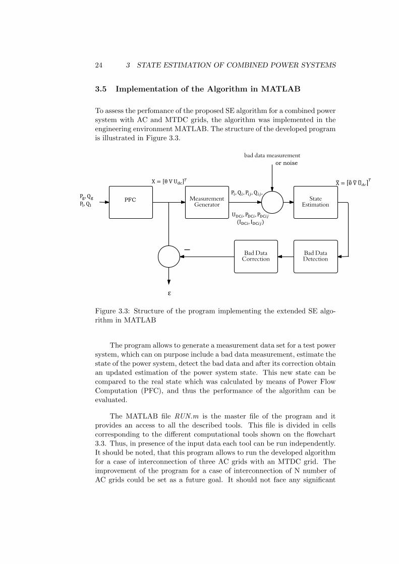
To assess the perfomance of the proposed SE algorithm for a combined powersystem with AC and MTDC grids, the algorithm was implemented in theengineering environment MATLAB. The structure of the developed programis illustrated in Figure 3.3.

X = [θ V U!"]! X! = !θ! V! U!!"!!

P! ,Q! ,P!" ,Q!" ,

U!"! , P!"! ,P!"!" (I!"! , I!"!")

P!,Q! P!,Q!

ε

PFC

or noise

Figure 3.3: Structure of the program implementing the extended SE algo-rithm in MATLAB

The program allows to generate a measurement data set for a test powersystem, which can on purpose include a bad data measurement, estimate thestate of the power system, detect the bad data and after its correction obtainan updated estimation of the power system state. This new state can becompared to the real state which was calculated by means of Power FlowComputation (PFC), and thus the performance of the algorithm can beevaluated.

The MATLAB file RUN.m is the master file of the program and itprovides an access to all the described tools. This file is divided in cellscorresponding to the different computational tools shown on the flowchart3.3. Thus, in presence of the input data each tool can be run independently.It should be noted, that this program allows to run the developed algorithmfor a case of interconnection of three AC grids with an MTDC grid. Theimprovement of the program for a case of interconnection of N number ofAC grids could be set as a future goal. It should not face any significant

3.5 Implementation of the Algorithm in MATLAB 25

obstacles, since the current program was written in a flexible and quitetransparent way. It is also important to stress out the fact that the programuses the per unit system (p.u.). Thus, all the input and output values arein p.u.

The input data required to run the complete program should be savedin the file Project TestData.mat and should include the following structurearrays:

1. topo 1, topo 2, topo 3 with the description of AC grids, namely thetopology description and parameters of each grid. The topology dataof an AC grid includes: number of the buses in the grid; start andend buses for each branch of the grid; index of the slack bus whichis chosen as a point of connection of the converter AC/DC interfaceto the AC grid. The input parameters of an AC grid should includeimpedances and shunt admittances of its branches; shunt addmitancesof the buses and tap ratios of the transformers.

2. topo dc with the description of the MTDC grid, namely its topologyand parameters. The topology data of a DC grid includes: numberof the buses in the grid; start and end buses for each branch of thegrid; index of the slack bus. The input parametrs of a DC grid areresistances of its branches.

3. pf input 1, pf input 2, pf input 3 which are matrices with the requiredinput data for the PFC for each AC grid. The following information isstored in these matrices: bus types (PU or PQ); active power injectionsfrom the generators; known active (for PU and PQ buses) and reactivepower injections (for PQ buses); known voltage magnitudes (for PUbuses).

To be able to test the algorithm, a feasible test data set should begenerated. This task is resolved by PFC which is carried out separatelyfor each grid. The corresponding MATLAB functions are run pf.m for ACgrids and pf dc.m for the MTDC grid. Both functions are controlled by themaster file.

The first computational step of the program is the preliminary PFC.This is required in order to obtain the values of the power that should begenerated in each AC system to meet the specified injections from the gridsto the MTDC grid. Since the PFC is run independently for each grid, thepreliminary values of power injections from each AC grid to the MTDCgrid should be obtained. The injections to two of the AC grids are enteredmanually in a corresponding dialog box, and the third injection is calculated


in pf dc.m function along with the power flows in the branches of the MTDCgrid. The values of the active power injections to AC grids from the MTDCgrid are then added to the power injection value of the converter AC sidebus stored in pf input X, where X is the number of the AC grid (1,2 or 3).Thus, at this step the power transmission via the MTDC grid is modelledas an additional active power load/generation in the converter AC side bus.To obtain the value of power generation required in an AC grid to keep itsactive power balance, the bus with the broadest generation range is set asa slack bus and run pf.m performs PFC. The results of the PFC are savedinto pf input X new matrices which have the same structure as pf input X.

At the next stage, the real state of the combined power system is cal-culated. Since the active power of each AC system of the combined grid isbalanced in a converter, a point of connection of the AC/DC interface toan AC grid is set as a slack bus for each AC system. The data stored inpf input X new is used as input for the new round of PFC. The output ofthe PFC for each AC grid is: the state vector state X new and the matricespflows X new and pinjections X new containing the values of active and re-active power flows and injections. The measurement generator saves the ACvoltage magnitudes, active power injections, reactive power injections andflows in the structures meas X of the Project TestData.mat. Besides that,the calculated DC values, such as DC voltages, DC current injections andflows and power injections and flows are saved into the structure meas dc ofthis file.

To perform the SE of a combined power system, the measurement anddata sets of the AC grids should be combined to obtain a complete data set.The topologies of the AC grids should be also joint in one structural vari-able. These two tasks are accomplished using of the file interconnect.m. Theresulting structure arrays meas and topo along with meas dc and topo dcare the input data for the WLS SE algorithm implemented in the StateEsti-mation.m function. The topology and parameters of the grids are processedwith the files admittance matrix.m and admittance matrix dc.m to createthe admittance matrices of the AC and MTDC parts of the combined grid.The SE is performed by means of the WLS SE algorithm with OrthogonalFactorization. The measurement function and the measurement Jacobianare calculated in the separate functions f measFunc h.m and f measJac Hwith the elements corresponding to the ones described in Sections 3.2.3 and3.2.4. The iterative SE runs until the required accuracy is obtained. If someof the redundant measurements predefined as an input data are not available,the SE algorithm tool will delete the corresponding entries of the measure-ment function and rows of the measurement Jacobian, thus performing theSE not requiring all the possible measurements to be available.

3.5 Implementation of the Algorithm in MATLAB 27

A single bad data measurement can be added in the obtained measure-ment data set. Another possible option is corruption of the measurementdata set by Gaussian noise. A corresponding dialog box allows to choosebetween a DC and AC bad data or addition of the noise. In case of a sin-gle bad data at the next step the program offers to define the type, thebus/branch of the faulty measurement, the relative change of the real value.The bad data is then detected by means of the residual analysis in thefunction BadDataDetection.m. The measurement with the largest normal-ized residual is deleted from the data set and the corrected state of thepower system is estimated at the step Bad Data Correction. The real andestimated states are compared by calculating the Normalized Root MeanSquared Error (NRMSE) of the estimation:

NRMSE =

√∑mi=1(xi − xi)2∑mi=1(xi − x)2

× 100% (3.38)

where x is a mean value of x.This allows to assess the perfomance of the program.

Among the figures that are output by default by the program are theAC voltage magnitudes, AC voltage angles and DC voltages of the real andestimated states (or real, corrupted by the bad measurement and correctedstates) and the visualization of the K-matrix obtained for the combined grid.As stated in section 3.3, the K-matrix can be used as a basis for definingthe critical measurements in the system.

28 4 CASE STUDY

4 Case Study

4.1 Case Study Description

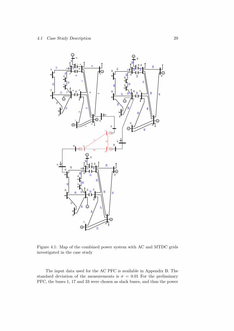
The combined grid considered in the case study consists of three IEEE 14-bus networks interconnected via MTDC 3-bus loop grid. Each IEEE 14-bus grid has 11 loads covered by 2 generators. The transmission grid isformed by 14 buses, 15 lines and 3 transformers. A shunt capacitor and 3synchronous compensators are installed in each AC grid in order to provideit with reactive power and support the voltage level [10].

The numeration of the buses of the MTDC grid corresponds to theindices of the AC grids connected to them. The map of the interconnectedpower system is shown in Figure 4.1. Each AC grid is extended to a 16-busgrid by adding the converter AC/DC interface circuit. The parameters ofthe three IEEE 14-bus systems, AC/DC interface elements, converters, andthe MTDC grid are listed in the Appendix A.

The state vector is as stated in Section 3.2.2, namely X = [θ V UDC]T .The number of the unknown variables in the state vector depends on thenumber of the interconnected AC grids and the number of the buses of eachAC grid and the MTDC grid. Since each AC grid has its own slack bus witha fixed value of the voltage angle, the number of the AC variables is equalto 2 ·nbusAC−NAC = 2 · (3 · (14 + 2))− 3 = 93. The number of the unknownDC variables is nbusDC − 1 = 2, because the voltage of the reference busshould be given. Thus, the total number of the unknown state variables is93 + 2 = 95. The slack buses can be chosen arbitrarily, though for the casestudy the following slack buses were chosen: AC 1 - bus 2; AC 2 - bus 30(14 in the original IEEE 14-bus grid); AC 3 - bus 38 (6 in the original IEEE14-bus grid); MTDC - bus 3.

The choice of the AC slack buses was made corresponding to the pointsof the connection of AC/DC interface circuits to the AC grids. In these nodesthe active and reactive power can be effectively controlled. The voltageangles of the AC slack buses are set to zero, the value of the DC voltage ofthe MTDC slack bus is set to 1.0 p.u. Thus, the voltage angles of the differentAC grids are independent from each other, and do not influence directly onthe states of the other grids. Though all the three grids are coupled via theMTDC grid which creates an interdependence of power flows between theAC networks.

4.1 Case Study Description 29

Figure 4.1: Map of the combined power system with AC and MTDC gridsinvestigated in the case study

The input data used for the AC PFC is available in Appendix B. Thestandard deviation of the measurements is σ = 0.01 For the preliminaryPFC, the buses 1, 17 and 33 were chosen as slack buses, and thus the power

30 4 CASE STUDY

generation in these buses was adjusted in order to preserve the power balancein each AC grid. The values of the active power injection from the convertersto the AC 1 and AC 2 grids were set to -1.0 p.u. and 0.6 p.u. correspondingly.That means that the power transmission is conducted from AC 1 to AC 2and AC 3. The value of the power injection to the AC 3 was calculatedusing DC PFC and is equal to 0.3776 p.u. The transmission of the powerbetween AC 2 and AC 3 is made in the direction from AC 3 to AC 2.

4.2 Case Study. Results of the State Estimation 31

4.2 Case Study. Results of the State Estimation

As stated in Sec. 3.5, the developed program allows to obtain the real stateof the combined power system using the PFC technique. Based on thisreal state, the measurement data set is generated, and afterwards the SEalgorithm is implemented.

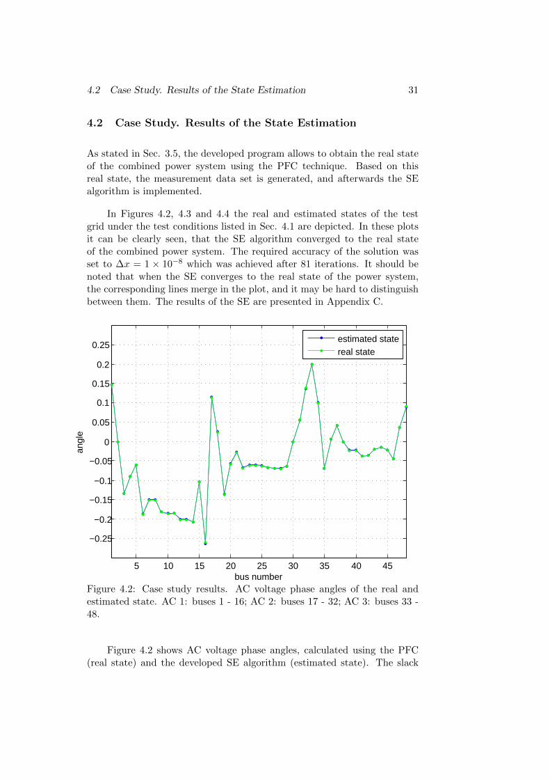
In Figures 4.2, 4.3 and 4.4 the real and estimated states of the testgrid under the test conditions listed in Sec. 4.1 are depicted. In these plotsit can be clearly seen, that the SE algorithm converged to the real stateof the combined power system. The required accuracy of the solution wasset to ∆x = 1 × 10−8 which was achieved after 81 iterations. It should benoted that when the SE converges to the real state of the power system,the corresponding lines merge in the plot, and it may be hard to distinguishbetween them. The results of the SE are presented in Appendix C.

5 10 15 20 25 30 35 40 45

−0.25

−0.2

−0.15

−0.1

−0.05

0

0.05

0.1

0.15

0.2

0.25

angl

e

bus number

estimated statereal state

Figure 4.2: Case study results. AC voltage phase angles of the real andestimated state. AC 1: buses 1 - 16; AC 2: buses 17 - 32; AC 3: buses 33 -48.

Figure 4.2 shows AC voltage phase angles, calculated using the PFC(real state) and the developed SE algorithm (estimated state). The slack

32 4 CASE STUDY

buses of the AC grids (2, 30, 38) can be easily determined from this plot -their phase angles are equal to zero. The location of the generating unitswith the highest power output is also clear from this picture: they are locatedat buses 1, 17 and 33, where the phase angles of the AC grids are the largest.

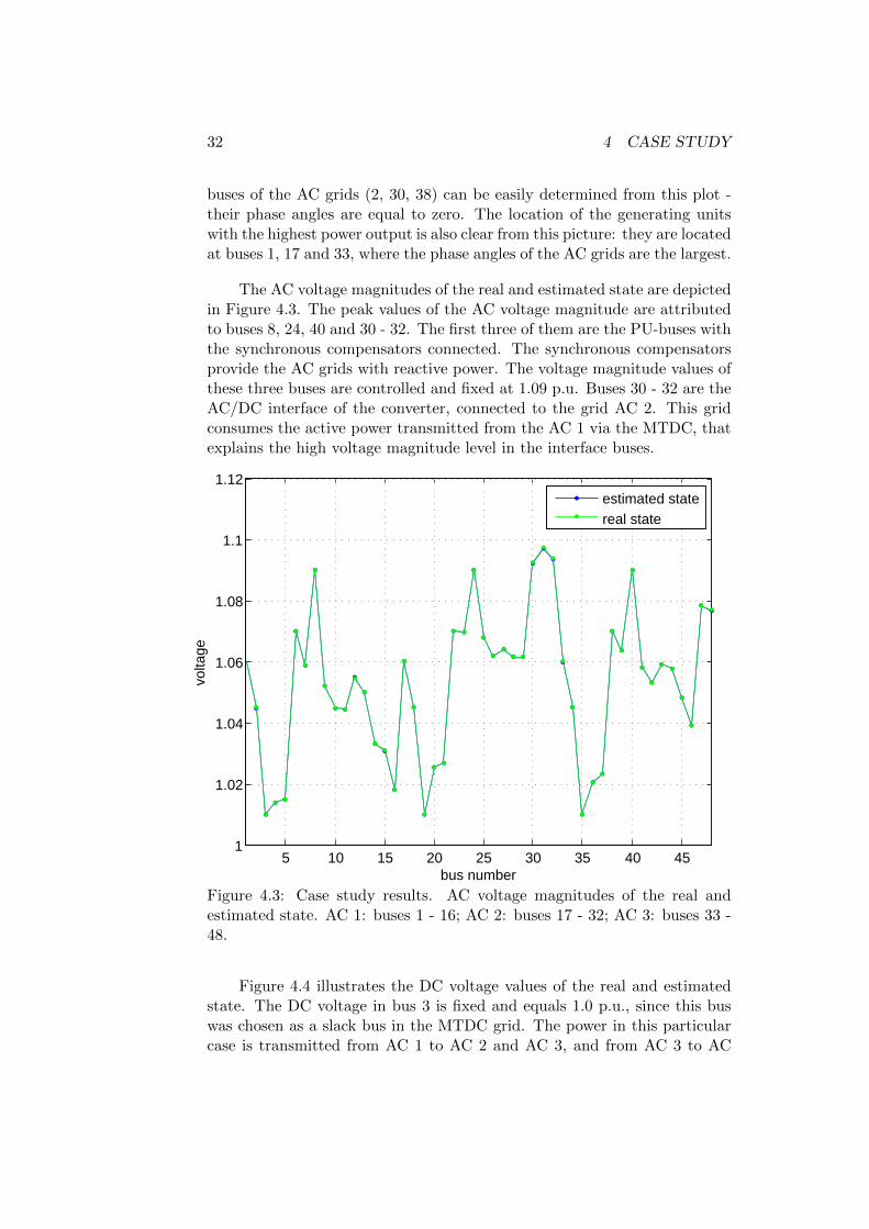
The AC voltage magnitudes of the real and estimated state are depictedin Figure 4.3. The peak values of the AC voltage magnitude are attributedto buses 8, 24, 40 and 30 - 32. The first three of them are the PU-buses withthe synchronous compensators connected. The synchronous compensatorsprovide the AC grids with reactive power. The voltage magnitude values ofthese three buses are controlled and fixed at 1.09 p.u. Buses 30 - 32 are theAC/DC interface of the converter, connected to the grid AC 2. This gridconsumes the active power transmitted from the AC 1 via the MTDC, thatexplains the high voltage magnitude level in the interface buses.

5 10 15 20 25 30 35 40 451

1.02

1.04

1.06

1.08

1.1

1.12

volta

ge

bus number


Figure 4.3: Case study results. AC voltage magnitudes of the real andestimated state. AC 1: buses 1 - 16; AC 2: buses 17 - 32; AC 3: buses 33 -48.

Figure 4.4 illustrates the DC voltage values of the real and estimatedstate. The DC voltage in bus 3 is fixed and equals 1.0 p.u., since this buswas chosen as a slack bus in the MTDC grid. The power in this particularcase is transmitted from AC 1 to AC 2 and AC 3, and from AC 3 to AC

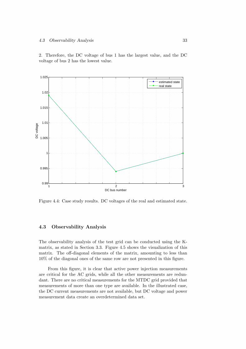
4.3 Observability Analysis 33

2. Therefore, the DC voltage of bus 1 has the largest value, and the DCvoltage of bus 2 has the lowest value.

1 1.2 1.4 1.6 1.8 2 2.2 2.4 2.6 2.8 30.99

0.995

1

1.005

1.01

1.015

1.02

1.025

DC

vol

tage

DC bus number


Figure 4.4: Case study results. DC voltages of the real and estimated state.


The observability analysis of the test grid can be conducted using the K-matrix, as stated in Section 3.3. Figure 4.5 shows the visualization of thismatrix. The off-diagonal elements of the matrix, amounting to less than10% of the diagonal ones of the same row are not presented in this figure.

From this figure, it is clear that active power injection measurementsare critical for the AC grids, while all the other measurements are redun-dant. There are no critical measurements for the MTDC grid provided thatmeasurements of more than one type are available. In the illustrated case,the DC current measurements are not available, but DC voltage and powermeasurement data create an overdetermined data set.

34 4 CASE STUDY

0 50 100 150 200 250

0

50

100

150

200

250

nz = 4095

matrix K (off−diagonal elements smaller than 1/10 of diagonal ones are neglected)

Figure 4.5: Visualization of K-matrix (off-diagonal elements smaller than0.1 of the diagonal of the same row are deleted)


Bad data was incorporated in the measurement set by adding a single baddata first in an AC measurement and then in a DC measurement, and bycorrupting the measurement data set by Gaussian noise. In the first twocases the bad data detection and correction algorithms were tested. Thenoise analysis allowed to assess the SE algorithm performance by calculat-ing the NRMSE of the states estimated for diverse values of the standarddeviation of the noise.


4.4.1 Bad Data in an AC measurement

In order to investigate the case of a single bad data in an AC measurement,the AC voltage magnitude at bus 27 was increased by 20%. The resultsof the Bad Data Detection and Correction are illustrated in Figures 4.6,4.7 and 4.8. Figure 4.6 shows that having a bad data in an AC voltagemagnitude measurement does not influence on the AC voltage phase anglevalues. The three lines representing the phase angles of the real, corruptedby bad data and corrected states merge together.

5 10 15 20 25 30 35 40 45−0.4

−0.3

−0.2

−0.1

0

0.1

0.2

0.3

0.4

angl

e

bus number

real stateestimated state with bad datacorrected state

Figure 4.6: Case study results. AC voltage phase angles of the real, cor-rupted with a single AC bad measurement and corrected state. AC 1: buses1 - 16; AC 2: buses 17 - 32; AC 3: buses 33 - 48.

36 4 CASE STUDY

By contrast, the AC voltage magnitude values of the state corruptedby a bad data display high values of discrepancy at buses of the AC 2.This is logical, since the bad data is contained in the AC voltage magnitudemeasurement at bus 27 that belongs to AC 2. This bad data does notinfluence on the voltage magnitudes of the other AC grids, since the ACvoltage values are decoupled via the MTDC grid.

5 10 15 20 25 30 35 40 451

1.02

1.04

1.06

1.08

1.1

1.12

1.14

volta

ge

bus number


Figure 4.7: Case study results. AC voltage magnitudes of the real, corruptedwith a single AC bad measurement and corrected state. AC 1: buses 1 - 16;AC 2: buses 17 - 32; AC 3: buses 33 - 48.

The DC voltages are not changed in the considered case. The couplingof the AC and MTDC grids is modelled by the balance pseudomeasurements.A change in the value of a voltage magnitude measurement can influence on


the values of reactive power injections and flows, and does not affect activepower injections and flows. Therefore, it has a negligible influence on theactive power balance equations and thus on the DC values.

1 1.2 1.4 1.6 1.8 2 2.2 2.4 2.6 2.8 30.99

0.995

1

1.005

1.01

1.015

1.02

1.025

DC

vol

tage

DC bus number


Figure 4.8: Case study results. DC voltages of the real, corrupted with asingle AC bad measurement and corrected state.

4.4.2 Bad Data in a DC measurement

As an example of a single bad data in a DC measurement, the increasementof the power injection at bus 2 of the MTDC grid by 15% was studied.

This bad measurement affects both AC and MTDC parts of the com-bined power system. Since the parts are coupled via the active power balance

38 4 CASE STUDY

equations, a change in the DC power injection value will lead to a changein the AC power injection value. The AC active power is coupled with ACvoltage angles which can be observed in Figure 4.9. The elimination of thefaulty measurement by the program allowed to obtain the new correctedstate converging to the real state of the power system.

5 10 15 20 25 30 35 40 45−0.4

−0.3

−0.2

−0.1

0

0.1

0.2

0.3

0.4

angl

e

bus number


Figure 4.9: Case study results. AC voltage phase angles of the real, cor-rupted with a single DC bad measurement and corrected state. AC 1: buses1 - 16; AC 2: buses 17 - 32; AC 3: buses 33 - 48.

Figure 4.10 depicts AC voltage magnitudes of the three states. Thereis a nonsignificant discrepancy between the voltage magnitudes of the realstate of AC 2 and the estimated state with a bad measurement. The largestdifference occurs for the buses of the AC/DC interface of AC 2. This dif-


ference is caused by the correlation between the voltage magnitude at theconverter AC-side bus and the active power balance in the converter. How-ever, the elimination of the faulty measurement from the data set allowedto obtain the corrected state converging to the real one.

5 10 15 20 25 30 35 40 451

1.02

1.04

1.06

1.08

1.1

1.12

1.14

volta

ge

bus number


Figure 4.10: Case study results. AC voltage magnitudes of the real, cor-rupted with a single DC bad measurement and corrected state. AC 1: buses1 - 16; AC 2: buses 17 - 32; AC 3: buses 33 - 48.

Since DC power injections are strongly correlated to the DC voltages,a change in the value of DC power injection caused a change in the valueof DC voltage at bus 2 (Fig. 4.11). The bad data correction tool of theprogram enabled the improvement of the estimation of this value.

40 4 CASE STUDY

1 1.2 1.4 1.6 1.8 2 2.2 2.4 2.6 2.8 30.99

0.995

1

1.005

1.01

1.015

1.02

1.025

DC

vol

tage

DC bus number


Figure 4.11: Case study results. DC voltages magnitudes of the real, cor-rupted with a single DC bad measurement and corrected state.

4.4.3 Measurement Data Set Corrupted by Noise

The developed algorithm should have a high performance level in presence ofthe communication noise. In order to evaluate the efficiency of the algorithm,the measurement data set was corrupted by Gaussian noise with differentstandard deviation values. For each value the NRMSE was calculated, andthe results are presented in Figure 4.12 and Table 4.1. The NRMSE valueswere extrapolated by a quadratic polynomial.

Obviously, the value of NRMSE of SE increases with increasing the


standard deviation of the added noise. However, this value did not exceed5% for the value of standard deviation equal to 10%. It can be concludedthat the performed noise analysis serves as a verification of the developedSE algorithm.

0.01 0.02 0.03 0.04 0.05 0.06 0.07 0.08 0.09 0.10

0.5

1

1.5

2

2.5

3

3.5

4

4.5

5

standard deviation

NR

MS

E

NRMSE valuesextrapolation of NRMSE values

Figure 4.12: The Normalized Root Mean Square Error of the SE algorithmfor different values of Gaussian noise standard deviation and the extrapola-tion curve

σ 0.01 0.02 0.03 0.04 0.05 0.06 0.07 0.08 0.09 0.1

NRMSE, % 0.242 0.8012 1.228 1.512 1.748 3.053 3.234 2.718 3.425 4.429

Table 4.1: The Normalized Root Mean Square Error of the SE algorithmfor different values of Gaussian noise standard deviation

42 5 DISCUSSION AND CONCLUSION

5 Discussion and Conclusion

In this thesis, the SE algorithm for a combined power system with ACand MTDC grids was presented. The existing models of the MTDC gridincorporation in SE technique were studied, and an approach to modellinga combined power system for SE was developed. Three functions of SE wereconsidered, namely observability analysis, SE solution and bad data analysis.The existing SE technique based on the WLS Orthogonal Factorization SEalgorithm for AC power systems was reviewed and extended for the case ofa combined power system. The proposed SE algorithm was implemented inMATLAB for the case of interconnection of three AC grids by an MTDCgrid. To assess the performance of the developed program, a case study wasconducted. As a test power system of a case study, an interconnection ofthree IEEE 14-bus grids via a loop MTDC grid was considered. Within thecase study, the SE of the power system, observability analysis and bad dataanalysis were implemented. The algorithm was validated by means of thenoise analysis.

The proposed algorithm enables the SE of a combined power systemwith high accuracy and a required level of computational performance. Thedeveloped program allows to generate a measurement data set via PFC,estimate a state of a combined power system and conduct an observabilityand bad data analysis. A single bad measurement can be definied andeliminated from the data set, and thus an erroneous state can be corrected.

Diverse objectives of the further research can be suggested. The imple-mentation of two SE functions which were not addressed in this thesis can bedone. These are the topology processor and parameter and structural errorprocessing. These computational tools shall play a significant role to main-tain a secure operation of a combined power system. Another possible taskis implementation of more complex models of the power system components.For instance, the VSC model can be improved by adding the operating areaconstraints. Furthermore, the program developed in MATLAB can be ex-panded to a general case of an interconnection of an unrestricted number ofAC grids.

APPENDIX A. TEST GRID PARAMETERS 43

Appendix A

Test Grid Parameters

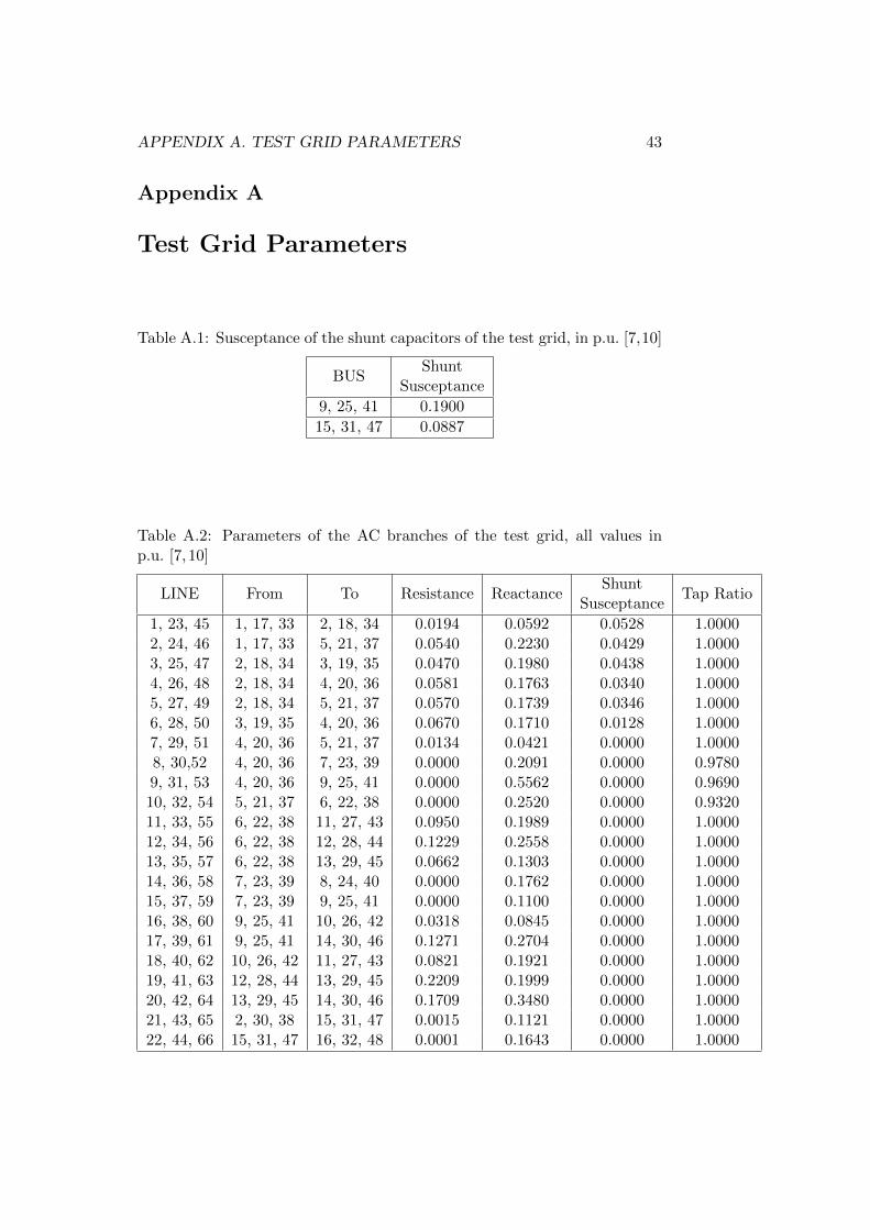
Table A.1: Susceptance of the shunt capacitors of the test grid, in p.u. [7,10]

BUSShunt

Susceptance

9, 25, 41 0.1900

15, 31, 47 0.0887

Table A.2: Parameters of the AC branches of the test grid, all values inp.u. [7, 10]

LINE From To Resistance ReactanceShunt

SusceptanceTap Ratio

1, 23, 45 1, 17, 33 2, 18, 34 0.0194 0.0592 0.0528 1.00002, 24, 46 1, 17, 33 5, 21, 37 0.0540 0.2230 0.0429 1.00003, 25, 47 2, 18, 34 3, 19, 35 0.0470 0.1980 0.0438 1.00004, 26, 48 2, 18, 34 4, 20, 36 0.0581 0.1763 0.0340 1.00005, 27, 49 2, 18, 34 5, 21, 37 0.0570 0.1739 0.0346 1.00006, 28, 50 3, 19, 35 4, 20, 36 0.0670 0.1710 0.0128 1.00007, 29, 51 4, 20, 36 5, 21, 37 0.0134 0.0421 0.0000 1.00008, 30,52 4, 20, 36 7, 23, 39 0.0000 0.2091 0.0000 0.97809, 31, 53 4, 20, 36 9, 25, 41 0.0000 0.5562 0.0000 0.969010, 32, 54 5, 21, 37 6, 22, 38 0.0000 0.2520 0.0000 0.932011, 33, 55 6, 22, 38 11, 27, 43 0.0950 0.1989 0.0000 1.000012, 34, 56 6, 22, 38 12, 28, 44 0.1229 0.2558 0.0000 1.000013, 35, 57 6, 22, 38 13, 29, 45 0.0662 0.1303 0.0000 1.000014, 36, 58 7, 23, 39 8, 24, 40 0.0000 0.1762 0.0000 1.000015, 37, 59 7, 23, 39 9, 25, 41 0.0000 0.1100 0.0000 1.000016, 38, 60 9, 25, 41 10, 26, 42 0.0318 0.0845 0.0000 1.000017, 39, 61 9, 25, 41 14, 30, 46 0.1271 0.2704 0.0000 1.000018, 40, 62 10, 26, 42 11, 27, 43 0.0821 0.1921 0.0000 1.000019, 41, 63 12, 28, 44 13, 29, 45 0.2209 0.1999 0.0000 1.000020, 42, 64 13, 29, 45 14, 30, 46 0.1709 0.3480 0.0000 1.000021, 43, 65 2, 30, 38 15, 31, 47 0.0015 0.1121 0.0000 1.000022, 44, 66 15, 31, 47 16, 32, 48 0.0001 0.1643 0.0000 1.0000

44 APPENDIX A. TEST GRID PARAMETERS

Table A.3: Resistance of the DC branches of the test grid, in p.u. [7]

LINE From To Resistance

1 2 2 0.052 2 3 0.063 3 1 0.04

Table A.4: Parameters of the model of active power losses in a converter [7]

Parameter a b c

Value 0.0053 0.0037 0.0018

APPENDIX B. TEST DATA SET 45

Appendix B

Test Data Set

Table B.1: Input data for PFC of AC 1 [10]

Bus Bus TypePi

[p.u.]Qi

[p.u.]V

[p.u.]PCk

[p.u.]

1 PU 2.5600 0.1690 1.0600 02 PU 0.1830 0.2970 1.0450 03 PU -0.9420 0.0440 1.0100 04 PQ -0.4780 0.0390 0 05 PQ -0.0760 -0.0160 0 06 PU -0.3120 0.0470 1.0700 07 PQ 0 0 0 08 PU 0 0.1740 1.0900 09 PQ -0.2950 -0.1660 0 010 PQ -0.0900 -0.0580 0 011 PQ -0.0350 -0.1180 0 012 PQ -0.0610 -0.0160 0 013 PQ -0.1350 -0.0580 0 014 PQ -0.1490 -0.0500 0 015 PQ 0 0 0 016 PQ 0 0 0 -1.0000

46 APPENDIX B. TEST DATA SET


Bus Bus TypePi

[p.u.]Qi

[p.u.]V

[p.u.]PCk

[p.u.]

17 PU 2.8049 -0.2416 1.0600 018 PU 0.1200 0.4085 1.0450 019 PU -1.2815 0.2164 1.0100 020 PQ -0.6856 0.0448 0 021 PQ -0.1128 -0.0084 0 022 PU -0.1522 0.0544 1.0700 023 PQ 0 0 0 024 PU 0 0.1635 1.0900 025 PQ -0.1999 -0.1407 0 026 PQ -0.0809 -0.0549 0 027 PQ -0.0222 -0.0100 0 028 PQ -0.0324 -0.0108 0 029 PQ -0.1943 -0.0674 0 030 PQ -0.1194 -0.0415 0 031 PQ 0 0 0 032 PQ 0 0 0 0.6000


Bus Bus TypePi

[p.u.]Qi

[p.u.]V

[p.u.]PCk

[p.u.]

33 PU 2.8049 -0.2416 1.0600 034 PU 0.1200 0.4085 1.0450 035 PU -1.2815 0.2164 1.0100 036 PQ -0.6856 0.0448 0 037 PQ -0.1128 -0.0084 0 038 PU -0.1522 0.0544 1.0700 039 PQ 0 0 0 040 PU 0 0.1635 1.0900 041 PQ -0.1999 -0.1407 0 042 PQ -0.0809 -0.0549 0 043 PQ -0.0222 -0.0100 0 044 PQ -0.0324 -0.0108 0 045 PQ -0.1943 -0.0674 0 046 PQ -0.1194 -0.0415 0 047 PQ 0 0 0 048 PQ 0 0 0 0.3776

APPENDIX C. STATE ESTIMATION RESULTS 47

Appendix C

State Estimation Results

Table C.1: Real and estimated DC voltages of the test grid, in p.u. Discrep-ancy in values.

BUSDC VoltageReal StateUDCi

DC VoltageEstimated State

UDCi

∆UDCi

1 1.0191 1.0191 02 0.9940 0.9940 03 1.0000 1.0000 0

Table C.2: Real and estimated voltage angles and magnitudes of AC 1.Discrepancy in the values.

BUS

Voltageangle,

Real Stateθi, [rad]

Voltageangle,

Estimated State

θi, [rad]

∆θi[rad]

Voltagemagnitude,Real StateVi [p.u.]

Voltagemagnitude,

Estimated State

Vi, [p.u.]

∆Vi[p.u.]

1 0.1469 0.1471 -0.0002 1.0600 1.0598 0.00022 0.0000 0.0000 0.0000 1.0450 1.0448 0.00023 -0.1348 -0.1346 -0.0003 1.0100 1.0099 0.00014 -0.0909 -0.0905 -0.0004 1.0140 1.0140 0.00005 -0.0606 -0.0602 -0.0004 1.0149 1.0148 0.00016 -0.1882 -0.1872 -0.0009 1.0700 1.0700 0.00007 -0.1509 -0.1501 -0.0008 1.0587 1.0587 0.00008 -0.1509 -0.1500 -0.0009 1.0900 1.0900 0.00009 -0.1820 -0.1811 -0.0009 1.0522 1.0521 0.000110 -0.1867 -0.1857 -0.0010 1.0446 1.0446 0.000011 -0.1856 -0.1845 -0.0010 1.0445 1.0445 0.000012 -0.2018 -0.2008 -0.0011 1.0547 1.0548 -0.000113 -0.2018 -0.2008 -0.0010 1.0500 1.0500 0.000014 -0.2082 -0.2071 -0.0011 1.0332 1.0332 0.000015 -0.1042 -0.1052 0.0010 1.0309 1.0306 0.000316 -0.2614 -0.2641 0.0027 1.0181 1.0179 0.0002

48 APPENDIX C. STATE ESTIMATION RESULTS


BUS

Voltageangle,


Voltageangle,

Estimated State

θi, [rad]

∆θi[rad]

Voltagemagnitude,Real StateVi, [p.u.]

Voltagemagnitude,

Estimated State

Vi, [p.u.]

∆Vi[p.u.]

17 0.1139 0.1151 -0.0012 1.0600 1.0601 -0.000118 0.0241 0.0254 -0.0013 1.0450 1.0451 -0.000119 -0.1380 -0.1368 -0.0012 1.0100 1.0101 -0.000120 -0.0583 -0.0572 -0.0011 1.0254 1.0255 -0.000121 -0.0283 -0.0271 -0.0012 1.0269 1.0269 0.000022 -0.0688 -0.0678 -0.0010 1.0700 1.0701 -0.000123 -0.0616 -0.0606 -0.0010 1.0695 1.0696 -0.000124 -0.0616 -0.0605 -0.0011 1.0900 1.0901 -0.000125 -0.0632 -0.0624 -0.0008 1.0678 1.0679 -0.000126 -0.0684 -0.0675 -0.0009 1.0619 1.0620 -0.000127 -0.0700 -0.0690 -0.0010 1.0640 1.0641 -0.000128 -0.0702 -0.0693 -0.0009 1.0616 1.0617 -0.000129 -0.0648 -0.0640 -0.0008 1.0617 1.0617 0.000030 0.0000 0.0000 0.0000 1.0925 1.0922 0.000331 0.0561 0.0554 0.0007 1.0975 1.0972 0.000332 0.1383 0.1367 0.0016 1.0938 1.0935 0.0003

APPENDIX C. STATE ESTIMATION RESULTS 49


BUS

Voltageangle,


Voltageangle,

Estimated State

θi, [rad]

∆θi[rad]

Voltagemagnitude,Real StateVi, [p.u.]

Voltagemagnitude,

Estimated State

Vi, [p.u.]

∆Vi[p.u.]

33 0.1988 0.1994 -0.0006 1.0600 1.0600 0.000034 0.0998 0.1004 -0.0006 1.0450 1.0450 0.000035 -0.0695 -0.0689 -0.0006 1.0100 1.0100 0.000036 0.0058 0.0063 -0.0005 1.0204 1.0204 0.000037 0.0406 0.0411 -0.0005 1.0235 1.0234 0.000138 0.0000 0.0000 0.0000 1.0700 1.0699 0.000139 -0.0232 -0.0226 -0.0006 1.0636 1.0636 0.000040 -0.0232 -0.0226 -0.0007 1.0900 1.0900 0.000041 -0.0383 -0.0377 -0.0006 1.0580 1.0581 -0.000142 -0.0357 -0.0353 -0.0006 1.0533 1.0533 0.000043 -0.0196 -0.0193 -0.0003 1.0590 1.0590 0.000044 -0.0153 -0.0152 -0.0001 1.0578 1.0578 0.000045 -0.0223 -0.0221 -0.0002 1.0484 1.0484 0.000046 -0.0452 -0.0448 -0.0004 1.0392 1.0392 0.000047 0.0366 0.0360 0.0006 1.0784 1.0783 0.000148 0.0900 0.0886 0.0014 1.0769 1.0768 0.0001

50 APPENDIX D. CD CONTENTS.

Appendix D

CD Contents

• Report

• LaTex-files

• Figures

• MATLAB-Scripts

• Literature

• Presentation

REFERENCES 51

References

[1] A. Abur, A.G.Exposito, “Power System State Estimation,” MarcelDekker, 2004

[2] A. Monticelli, “State Estimation in Electric Power Systems,” Springer,1999

[3] M. Ahmad “Power System State Estimation,” Artech House, 2013

[4] M. Zima, M. Bockarjova, “Operation, Monitoring and ControlTechonology of Power Systems,” EEH - Power Systems Laboratory,ETH Zurich, 2014

[5] A. de la Villa Jaen, E. Acha, A. G. Exposito, “Voltage Source ConverterModeling for Power System. State Estimation: STATCOM and VSC-HVDC,” IEEE Transactions on Power Systems, Vol. 23, pp. 1552-1559,2008

[6] H.R. Sirisena, E.P.M. Brown, “Inclusion of HVDC Links in AC power-system State Estimation,” IEEE PROC, Vol. 128, pp. 147-154, 1981

[7] J.Cao, W. Du, H.F. Wang, “The Incorporation of Generalized VSCMTDC Model in AC/DC Power System State Estimation,” SustainablePower Generation and Supply, 2012

[8] Z. Chen, C. Liu, P. Tian, H. Li, W. Wang, “Observability Analysis ofPower System Including VSC-HVDC,” Sustainable Power Generationand Supply, 2012

[9] E.Caro, A.J. Conejo, ”State Estimation via Mathematical Program-ming: a Comparison of Different Estimation Algorithms,” IET Gener.Transm. Distib., Vol. 6, pp. 545-553, 2012

[10] University of Washington. Power systems test case archive.http://www.ee.washington.edu/research/pstca/

state estimation in power systems with combined ac … · state estimation in power systems with...

Documents