V I R G I N I A POLYTECHNIC INSTITUTE AND STATE U N I V E R S I T Y

E N G I N E E R I N G SCIENCE AND MECHANICS DEPARTMENT

BLACKSBURG, V I R G I N I A 24061

A Progress Report on

I D E N T I F I C A T I O N AND CONTROL OF STRUCTURES I N SPACE

NASA Research Grant NAG-1-225

Covering t h e Per iod

July 1 - December 31, 1935

(NASA-Cfi-I798 11) IDENTXFZCATION AND CONTROL N87-10172 O F S T R U C T U R E S IN EEACE Proqress Report, 1 J u l . - 31 Eec. 19E5 { V i r g i n i a P c l y t e c h n i c Inst. and S t a t e Uxiiv.) 42 p CSCL 22B Unclas

G3/18 44339

P r i n c i p a l I n v e s t i g a t o r : Leonard M e i r o v i t c h U n i v e r s i t y D is t i ngu ished Pro fessor

https://ntrs.nasa.gov/search.jsp?R=19870000739 2019-02-07T00:17:26+00:00Z

Abst rac t

Work d u r i n g t h e p e r i o d J u l y 1 - December 31, 1985, has concentrated

on t h e a p p l i c a t i o n o f t h e equat ions d e r i v e d i n t h e preceding p e r i o d t o

t h e maneuveri ng and v i b r a t i o n suppression o f t h e Spacecraf t Contro l

Laboratory Experiment (SCOLE) model. Two d i f f e r e n t s i t u a t i o n s have been

considered: 1) a space environment and 2 ) a l a b o r a t o r y environment.

Th is r e p o r t covers t h e f i r s t case and c o n s i s t s o f a paper e n t i t l e d

"Maneuveri ny and V i b r a t i on Control o f F1 e x i b l e Spacecraf t " , presented a t

t h e Workshop on S t r u c t u r a l Dynamics and Cont ro l I n t e r a c t i o n o f F l e x i b l e

S t ruc tures , Marshal l Space F l i g h t Center, H u n t s v i l l e , AL, A p r i l 22-24,

1986. The second case w i l l be covered i n t h e r e p o r t for t h e next

per iod.

MANEUVERING AND V I B R A T I O N CONTROL OF FLEXIBLE SPACECRAFT*

L. M e i r o v i t c h t & R. 0. Quinni-

V i r g i n i a Po ly techn ic I n s t i t u t e & S t a t e U n i v e r s i t y

Department o f Engineer ing Science & Mechanics

Blacksburg, V i r g i n i a 24061

* Supported by t h e NASA Research Grant NAG-1-225 sponsored by t h e Spacecra f t Cont ro l Branch, Langley Research Center.

t U n i v e r s i t y D is t i ngu ished Professor . Fe l l ow A I A A .

tt Graduate Research Ass is tan t . Now A s s i s t a n t Professor , Department of Mechanical and Aerospace Engineering, Case GIestern Reserve Un:’ver- s i t y , Cleveland, OH, 44106.

ABSTRACT

This paper is concerned with slewing a

suppressing any vibration at the same time.

undergo large rigid-body motions and small e

arge structure in space and

The structure is assumed to

astic deformations. A

perturbation method permits a maneuver strategy independent of the

vibration control. Optimal control and pole placement techniques,

formulated to include actuator dynamics, are used to suppress the

The theory is illustrated by simultaneous

control of the Spacecraft Control Laboratory

n a space environment.

vibration during maneuver

maneuvering and vibration

Experiment (SCOLE) model

I. INTRODUCTION

The problem of simultaneous maneuver and vibration suppression of

spacecraft is becoming increasingly important.

missions involve experiments consisting of the control of flexible

bodies carried by a shuttle in an earth orbit. Other missions involve

laboratory simulations o f similar experiments. The equations o f motion

for both types of experiments have been presented previously (Ref. 1).

A perturbation technique permitting the maneuver strategy to be

Some projected NASA

formulated independently of the vibration problem was also presented.

In a following investigation, a straightforward rotational maneuver

strategy and an efficient vibration simulation technique were presented

(Ref. 2). Rotational maneuvers were shown to cause structural

vibrations.

these vibrations during the maneuver by means of feedback control.

The purpose of this paper is to develop ways o f suppressing

Turner and Junkins (Ref. 3), Turner and Chun (Ref. 4) and Breakwell

(Ref. 5) addressed the problem of rotational maneuvering and

simultaneous vibration suppression of flexible spacecraft for two-

I

dimensional models. In all cases, the methods used represent extensions

o f rigid-body maneuvering techniques, requiring the solution of a two

point boundary-value problem. The maneuver and vibration control

problems are coupled and numerical difficulties arise as the order o f

the system increases (Ref. 5). Baruh and Silverberg first suggested

separating the maneuver and vibration control problems (Ref. 6).

However, the vibration control did not include feedback on the rigid-

body modes, so that the spacecraft orientation could not be corrected

during the open-loop maneuver.

The equations of motion of a flexible spacecraft consist of six

nonlinear ordinary differential equations for the rigid-body motion of a

reference frame attached to the spacecraft in undeformed state coupled

with a set of partial differential equations for the vibration of the

elastic members relative to the rigid frame. Hence, the equations

describing the motion o f a flexible spacecraft during a certain maneuver

represent a set of nonlinear hybrid differential equations. In general,

hybrid systems of equations do not permit closed-form solution, so that

one must consider an approximate solution, which implies spatial

discretization and truncation.

The nonlinear equations of motion can be solved by a perturbation

approach.

of equations for the rigid-body motions, representing zero-order

effects, and a set of equations for the small elastic motions and

deviations from the rigid-body motions, representing first-order

effects.

independent of the elastic vibration.

The approach consists of separating the equations into a set

The perturbation technique permits a maneuver strategy that is

The order o f the perturbation equations for the vibration

suppression is often so large that some reduction is necessary. To this

end, the elastic motion can be expanded into a series consisting of

premaneuver eigenvectors acting as admissible vectors.

vectors clearly do not decouple the equations of motion, but using a

smaller number than the order of the system permits a reduction in the

order. We refer to the corresponding equations as quasi-modal

equations. The task o f simulation and vibration control can be carried

out conveniently by means o f the quasi-modal equations.

These admissible

At each sampling time, the control forces are formulated as if the

premaneuver eigenfunctions are the true eigenfuctions at that time.

This results in a modeling error, but this error does not create a

stability problem for robust control techniques, such as natural

control, which do not require the exact eigenfunctions in control

formulation (Refs. 7-11).

Any maneuver can be regarded as a single-axis rotation, where in

general the axis of rotation is not a principal axis. The single-axis

maneuver has the advantage o f simplifying the matrices o f time-dependent

coefficients in the perturbation equations. The rigid-body maneuver

represents an open-loop control strategy for minimum-time, single-axis

rotation about an axis which i s not necessarily a principal axis.

The vibration control is carried out in discrete time, which

amounts to regarding the system as having constant coefficient over the

duration of any sampling period.

algorithms developed for time-invariant systems, such as optimal control

and pole placement. Actuator dynamics can degrade the performace of the

control system. The inclusion of actuator, dynamics requires a

This permits the use of control

reformulation of the vibration control techniques mentioned above. The

theory is illustrated by simultaneous maneuvering and vibration control

of the SCOLE model in a space environment.

11. E Q U A T I O N S OF MOTION

We consider a space system consisting o f a shuttle carrying an

antenna connected to the shuttle by means of a mast, as shown in Fig.

1. The shuttle is assumed to be rigid and the mast and antenna are

deformable. The motion of the spacecraft is referred to a given

reference frame xoyozo embedded in the rigid shuttle (Fig. 1).

reference frame has six degrees o f freedom, three rigid-body rotations

and three rigid-body translations. We propose to derive the equations

of motion by means of the Lagrangian approach, which requires the

expressions for the kinetic energy, potential energy and virtual work.

Considering Fig. 1, the position of a point S in the rigid shuttle

relative to the inertial frame X Y Z is RS I = R - + r. - Moreover, the position

of a point A on the elastic appendage is RA - = R - + a - + u, I where u I i s the

The

R = R + w x r -s - I I

elastic displacement. The velocities of these points are then

(1)

R - A = R + w x ( a + u ) + i - - I I

where R and w are the translational and angular ve

xoyozo with respect to the inertial frame, respect

elastic velocity of the point relative t o xoyozo.

energy of the spacecraft is

I

(2 )

ocities o f the fram

vely, and I is the

Hence, the kinetic

I

where mS and mA are the masses of the shuttle and appendage,

respectively.

The potential energy i s due to the combined effects of gravity and

strain energy. The gravitational potential can be expresssed as

where me is the mass of the-earth and G is the universal gravitational

constant. The strain energy can be expressed as an energy inner product

denoted by [ , ] (Ref. 12). This includes centrifugal and gravitational

stiffening effects on the appendage. The total potential energy then

becomes

( 5 ) 1 2 - - 9

- A

v = -[u,u] + v Denoting by fS - and f the force vectors per unit volume of the shuttle

and appendage, respectively, we can express the virtual work as

S W = J fS*6Rs - dDS + J dDA n - n

"A

where DS and DA are the domains of the shuttle and appendage,

respectively. The system is discretized in space by expressing the

elastic displacements vector in the form

u = #q ( 7 ) -., - where # is a matrix o f space-dependent admissible functions and q .. is a

vector o f time-dependent generalized coordinates. The kinetic and

potential energies and virtual work can be expressed in matrix form by

introducing a rotational transformation matrix C from the XYZ frame to

the xoyozo frame, where the elements o f C are nonlinear functions of a

set of Euler angles a l , a 2 , a3.

be written in the symbolic form

Lagrange's equations o f motion can then

d aT aV T - (-) + - = C F aR - dt aR

a(7)--+-- d aT aT a V - ag 3 9 -

a!!

where the matrix D is defined by the expression

The resulting equations o f motion are nonlinear due to the large rigid-

body motion.

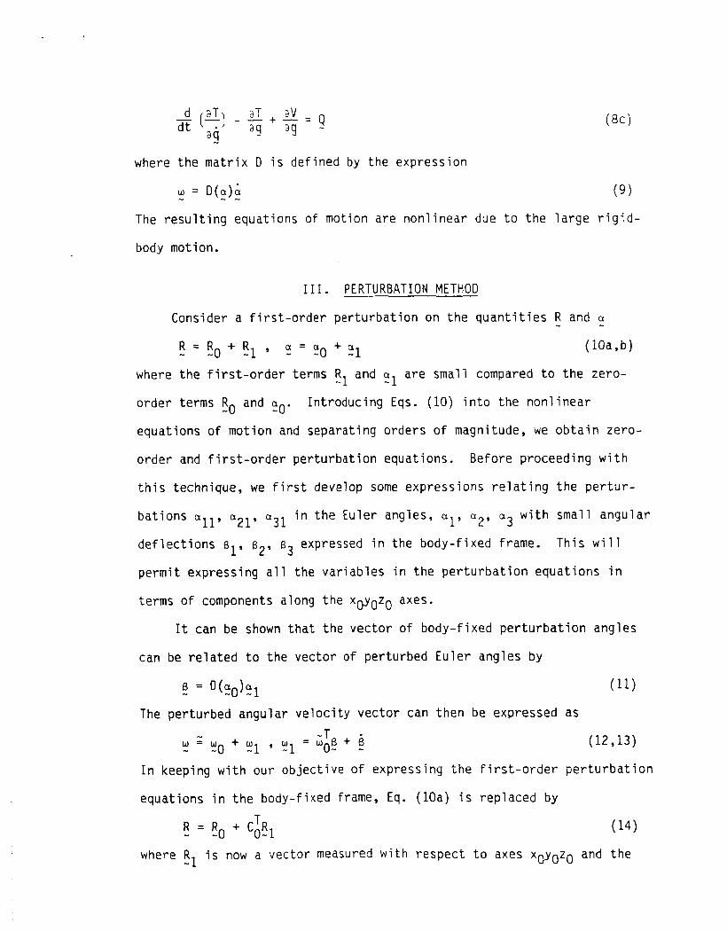
111. PERTURBATION METHOD

Consider a first-order

R = R o + F I 1 , - ! = a -0

where the first-order terms

perturbation on the quantities R - and Q

+ a (106, b -1 R and Q are small compared to the zero- -1 -1

order terms Ro - and ao. - equations of motion and separating orders of magnitude, we obtain zero-

Introducing Eqs. (10) into the nonlinear

order and first-order perturbation equations. Before proceeding with

this technique, we first develop some expressions relating the pertur-

in the Euler angles, al, a2, a3 with small angular a21' a31 bations all,

deflections ol, B ~ , B~ expressed in the body-fixed frame. This will

permit expressing all the variables in the perturbation equations in

terms of components along the xoyozo axes.

It can be shown that the vector of body-fixed perturbation angles

can be related to the vector of perturbed Euler angles by

The perturbed angular velocity vector can then be expressed as

In keeping with our objective of expressing the first-order perturbation

equations in the body-fixed frame, Eq. ( l o a ) is replaced by T R = Ro + C R - 0- 1

where R is now a vector measured with respect to axes xoyozo and the -1

r o t a t i o n m a t r i x has t h e per turbed form

?

( 1 5 0 ) 0 c co + c1 , c1 = gc The app l i ed f o r c e s and moments can a l s o be expressed i n f i r s t - o r d e r

per tu rbed form as f o l l o w s :

The zero-order equat ions o f mot ion, which govern t h e s t r u c t u r e as

i f i t were r i g i d , can be expressed as

T" - T-T" Gme A ^ T T T rnRo - + C S w + C o ~ o S o ~ o + ~ [ m R 0 + ( I - 3R R ) C S ] = CoFo 0 0-0 3 - -0-0 0-0

(17a) I!,I

"T .. Gme S -T C R + Io io

I Rol S C R + - 0 0-0 3 0 0-0

,. where Ro i s a u n i t v e c t o r i n t h e d

o f i n e r t i a m a t r i x about p o i n t 0, m

-T + W I W 0 0-0 - - Mo

r e c t i o n o f Ro, - Io i s t he mass moment

i s t he mass o f t he spacec ra f t and

The f i r s t - o r d e r l i n e a r p e r t u r b a t i o n equat ions, which govern t h e

v i b r a t i o n a l mot ion o f t he s t r u c t u r e , can be expressed i n t h e m a t r i x fo rm *

Mx + G i - + (Ks + KNS)x - . . , = F

where

M = [; -T

-

IO -T Q Lo

0 m 0

(19)

I

f I

and

T- 2 w 0 0 -T- 1

L J,

+ S o [ w o "T -2 + Fi] WoIoWo

I (0 = I (D dmA, Q -

mA

IV. RIGID-BODY MANEUVER

The perturbation method permits the maneuver strategy to be

designed independently o f the vibration control.

forward single-axis minimum-time maneuver strategy is developed in Ref.

2. It is shown in Ref. 2 that the axis of rotation need not be a

principal axis, so that any general rotational maneuver is possible.

The maneuver policy is formulated in continuous time but implemented in

discrete time, so t h a t seme error can nccuri

Indeed, a straight-

Also, the equations

governing the maneuver are nonlinear, so that the solution of Ref. 2 can

be unstable. However, the vibration control nciudes feedback control

of the rigid-body modes and can stabilize the spacecraft as well as

reduce the error caused by discrete-time samp ing.

The most desirable control technique for a maneuver excites only

the desired rigid-body motion, not the elastic modes. From Ref. 2, the

components of the maneuver force distribution exhibiting these

characteristics can be expressed as

( 22a)

where e(t) is the desired angular motion, m(p) is the mass density at

point p, and x(p), y(p) and z(p) are the components of the position

vector of point p with respect to the center of rotation.

forces are proportional to rotational rigid-body modes, so that they

will not excite the elastic modes and cause undesirable vibration. Of

course, distributed forces can only be implemented approximately with

discrete actuators, which tends to excite some vibration. Also,

centrifugal forces can cause vibration during the maneuver, so that

vibration control may be necessary.

The actuating

V. QUASI-MODAL EQUATIONS OF M O T I O N

During the maneuver, the gyroscopic and stiffness matrices, and

hence the eigenvalue problem, are functions of time. In Ref. 2, a

truncated set o f the premanetiver eigenvectors is iised as a set of

admissible vectors to simplify and reduce the order o f the equations of

motion t o a form called the quasi-modal equations of motion.

approach, Eq. (19) can be reduced to the quasi-modal form

Using this

f I

I

u(t) + G(t)i(t) + [ A + K(t)]u(t) = f(t)

where - -

T T G(t) = X G(t)X, K(t) = X Kt(t)X

are reduced-order gyroscopic and stiffness matrices, u is a vector of

the quasi-modal coordinates defined by -

x(t) - = Xu(t) - (244

where X is a rectangular matrix of the lower premaneuver eigenvectors

normalized so that T T X M X = I , X K O X = A

in which KO contains the constant terms in the stiffness matrix and A is

a diagonal matrix o f the premaneuver eigenvalues, and

f(t) = XTF*(t) (24f)

is the vector of modal forces. Comparing Eq. ( 2 3 ) with Eq. (19), we see

that the premaneuver eigenvectors have not decoupled the equations of

motion. However, as the maneuver velocity decreases, the time-varying

terms decrease in magnitude and the equations approach an uncoupled

form. Also note that the mass matrix has been reduced to the identity

matrix, which is convenient for casting Eq. (23) in state space form.

VI. VIBRATION CONTROL

The tangential and centrifugal disturbance forces during the

maneuver can cause vibration to be suppressed by means of feedback

control, as demonstrated in Ref. 2. The perturbation method permits the

vibration control to be formulated separately from the maneuver control,

resulting in the quasi-modal equations of ~o i i c j f i .

a) Actuator Dynamics

The equation of motion for the rth mode can be expressed as

(25 ) ur(t) + urur(t) 2 = fdr(t) + fr(t)

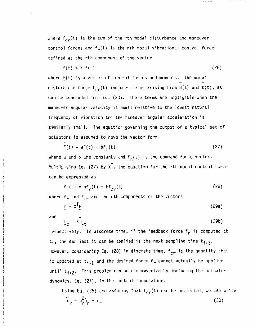
where fdr(t) i s the sum of the rth modal disturbance and maneuver

control forces and fr(t) is the rth modal vibrational control force

defined as the rth component of the vector

f(t) = XTF(t) (26)

where F(t) i s a vector of control forces and moments. The modal

disturbance force fdr(t) includes terms arising from G(t) and K ( t ) , as - - -

can be concluded from Eq. (23). These terms are negligible when the

maneuver angular velocity is small relative to the lowest natural

frequency o f vibration and the maneuver angular acceleration is

similarly small.

actuators is assumed to have the vector form

The equation governing the output of a typical set of

F(t) * = aF(t) - + bFc(t) (27)

where a and b are constants and Fc(t) - is the command force vector.

Multiplying Eq. (27) by XT, the equation for the rth modal control force

can be expressed as

fro) = afr(t) + bfcr(t) (28)

where f, and fcr are the rth components of the vectors

(29a) T f = X F ... - T

fc - = X Fc - and

respectively.

ti, the earliest it can be applied i s the next sampling time ti+l.

However, considering Eq. (28) in discrete time, fcr is the quantity that

is updated at ti+l and the desired force fr cannot actually be applied

until ti+2.

dynamics, Eq. (27) , in the control formulation.

In discrete time, if the feedback force fr is computed at

This problem can be circumvented by including t h e actuator

Using Eq. (25) and assuming that fdr(t) can be neglected, de can write 2. r r r

... u r + w u = f

Then, introducing Eqs. (25) and

equation can be expressed as 2 - 2 r r r r

... ur = - W u + aur + aw u

Equation (31) can be rewritten

z = Artr + bfcr -r %

where T T

2 = [Ur ur Ur] , b = -r

A = r

r

1

0

2 r --w i: a

(28) into Eq. ( 3 0 ) , the combined dynamic

+ bfcr n the state form

b) Optimal Control

The minimum-time optimal control policy i s bang-bang and involves

determining three-dimensional switching surfaces for each mode.

sampling time the modal state is to be located with respect to the

switching surfaces, and based on this the command modal force is set at

the positive or negative maximum value. The calculation of three-

dimensional switching surfaces is not a simple matter and using them in

the above mentioned fashion can be computationally time consuming (Ref.

13). If the measured modal states are noisy, the modal forces could be

switched frequently. This implies frequent, abrupt structural

accelerations which, when applied with spatially-discrete forces, tend

to destabilize the uncontrolled modes.

A t each

As an alternative, we consider a quadratic performance measure in

conjunction with the independent modal-space control (IMSC) method. In

particular, we consider a performance index consisting of a weighted sum

of the elastic energy and the control effort (Refs. 8, 9).

per-formarice index has t h e form

This -

m

J = z Jr r= 1

( 3 4 )

where

!

t

Jr = (z'Q -r r-r z + Rrfgr)dt (35)

are modal performance indices, in which

is a weighting matrix and R, is a weighting factor.

modes, qr is taken as the rth eigenvalue wr, and for the rigid-body

modes qr is chosen on the basis of pole-placement considerations.

the weight Rr is decreased, the rate of modal energy dissipation is

increased and, of course, more effort is required.

chosen on the basis of the available control command force for vibration

suppression. The command forces required by this performance index tend

For the elastic 2

As

Hence, R, can be

t o be smooth functions.

that they do not tend to excite the uncontrolled modes to the extent

Smooth forcing time histories are preferable in

that forces containing discontinuities do.

To minimize J, each modal performance index Jr can be minimized

independently. The steady-state Riccati equation for the rth mode i s an

algebraic matrix equation of order three and can be expressed as

1 I + - K bb Kr I 0 = -K A - ArKr - Q, r r Rr r-- ( 3 7 )

where Kr is a symmetric matrix to be determined; the matrix has the form

The linear, state feedback control law i s of the form

bTK z - fer - - - Rr - r-r

Introducing Eqs. (33a,b) into Eq. (39)’ the control law becomes

(39)

which minimizes the performance index given by Eq. (35) (Ref. 13). In

solving Eq. (37), the required entries o f Kr can be shown to satisfy the

following expressions:

= Rr (a,: + dr) kr3 b

k 4 C + k 3 C + k 2 C t k r 6 C 1 + C o = 0 r6 4 r6 3 r6 2

- b2 2 kr5 - -akr6 + - 2Rr kr6 where

1 W r 3 - 7 )

+ a’)

2 4 2 1

1 2 b2

1 dr 2 2drRr (,r

dr = [a w r + qrb /R,]’/2, c = - O dr

C = - - (d + a$, C = ~

c = - b a 4 b6 c = - 2d r r R2’ 4 8drR:

are constant coefficients which can be evaluated for each mode off-

line. The control law given by Eq. (40) is IMSC modified to include

actuator dynamics. IMSC is also called natural control because the

closed-loop modes are identical to the open-loop or natural modes, so

that natural coordinates remain natural after control (Ref. 9). Natural control j s effjcjent because i t 1.13cto

v.u-lcL-s n2 e f f e r t i n c h m i n g t h e shape

of the modes (Ref. 14), as other control techniques do. In this regard,

we recall that only eigenvalues affect stability and not eigenvectors.

Equation (40) can be expressed in the form - fer - -grlUr - gr2'r - gr3'r

where the control gains are defined as follows:

(43)

(44a-c)

Introducing Eq. (43) into Eq. (32), considering Eqs. (33) and expanding

the characteristic determinant, we conclude that the closed-loop poles

must satisfy the equation

c) Pole Allocation

In optimal control, a performance measure is defined, perhaps

arbitrarily, and minimized. The pole-allocation method is a modal

control method in which the poles are chosen for each mode, again

somewhat arbitrarily, and the actuator forces are computed to produce

these preselected poles. The most general form of the poles for the rth

mode defined by Eqs. (32) and (33), and whose characteristic equation i s

represented by Eq. (45), can be expressed as

= a - ie,, sr3 - - yr (46a-c) = a + iBr, sr2 r 'rl r where or and y r are related to the time constants for the rth mode

and B, is the closed-loop modal frequency.

associated with the poles given by Eqs. (46) is

The characteristic equation

3 2 2 2 2 2 s + (-y r - 2ar)s + (2yrar + ur + B,)S + (-yrar - y,~,) = o (47) Comparing Eqs. (47) and (45), we obtain the control gains

Hence, the poles given by Eqs . (46) can be chosen for each mode and

implemented with the command modal force given by Eq. (43) and the gai rs

of Eqs. (48).

d) Implementation of Modal Control

i. Modal actuation

Implementation of any IMSC technique requires an inversion of Eq. '

(29b), so that the applied command force Fc can be found from knowledge of the modal command force f . For discrete actuators, the simplest

implementation technique is a projection method (Ref. 9). Premulti-

plying Eq. (24d) by the pseudo-inverse of XT, denoted by X-T, we obtain

-C

X-T = MX (49)

Ec = MXf -C (50)

Premultiplying Eq. (29b) by X-T and considering Eq. (49), we obtain

which is the discrete counterpart o f a distributed generalized force and

must be applied with actuators at every finite element node. This may

require an impractically large number of actuators, so that only an

approximate "distributed" force can be applied. In the projection

technique, distributed control is implemented approximately by means of

discrete actuators (Ref. 9).

Another method of calculating the applied command force cc requires The advantage of this technique is that a numerical inversion (Ref. 8).

it produces a subset of the desired components of the modal force vector

exactly, rather than only approximately as in the case of projected

control. Hence, this type o f Control i s a true natural control i n that

the closed-loop eigenfunctions of the controlled modes are identical to

the open-loop eigenfunctions.

recalculated in the event of an actuator failure. The forces computed

Note that the inversion must be

i

from both the inverse and projected methods tend to excite the

uncontrolled modes giving rise to so-called control spillover (Ref. 8,

9 ) -

ii. Modal estimation

Modal state estimation is another common problem inherent in the

implementation of modal control techniques. This problem is somewhat

analogous to that of modal force implementation. It requires the

estimation of u(t) from measurement of x(t), which requires premulti- - - plication of Eq. (24c) by the matrix product X'M, so that

u(t) = XTMx(t) (51)

which is the second half of the expansion theorem (Ref. 12).

(51) and its time derivatives form what are known as modal filters (Ref.

15). Application of modal filters presupposes either "distributed"

sensors or sensors at every node for a finite element model.

acceptable approach to modal state estimation is to interpolate the

discrete sensor measurements by means of admissible functions to produce

approximate displacement and velocity profiles, where the latter are

functions of the spatial variables. These functions are then introduced

into the modal filter equations to yield the approximate modal states.

Equation

An

An alternative approach to modal state estimation involves a

numerical inversion of a matrix. In a manner analogous to the inversion

technique for force implementation, the displacement vector and modal

matrix of Eq. (24c) can be partitioned as follows:

where x

complement of xs, I Bs is an s x c submatrix of the modal matrix X and B,,

i s the complement of Bs.

i s an s x 1 vector of measured displacements, x~~ is the - S

Hence, the equation

x - S = B s u (53)

relates the modal displacements with the measured displacements.

Premultiplying Eq. (52) by B;', we obtain

u = B-lx s - s where 6,' is only a pseudo-inverse of B, if s t c . The expression

1 x = B B - x -ns ns s - s

( 5 4 )

(55)

can be regarded as observation spillover. Equation (55) implies

assignment of values to the unmeasured components of the displacement

vector.

e) Output Feedback Control

Modal control techniques have become quite common in the field of

control of structures because of their ability to take advantage of the

physical and mathematical properties of the natural modes of vibration.

The main drawback common to all modal control methods is the problem

encountered in modal state estimation with discrete sensors. Direct

feedback, where the command control force is related directly to the

measured state through control gains, avoids modal estimation

entirely. In addition, if this feedback force is the physical (rather

than modal) force, then the modal force implementation is also

avoided. Hence, a useful control technique might take advantage of the

concepts o f naturai mocies but be applicabie to output feedback. To this

end, the relationship between linear, output feedback control and linear

modal feedback control will now be explored.

Consider a linear control law having the special form

F -C (t) = -A[gt)gl + -(t)g, + :(t)g31 ( 5 6 )

where gl, g2 and g3 are control gain factors, Fc i s a vector o f actcal

command forces, x,

and accelerations and A i s a weighting matrix of constant coefficierts.

Using Eq. (24c) we obtain

- and x vectors o f measured displacements, velccities - - -

F -C (t) = -AX[u(t)g1 + !(t)g* + ij(t)g31 ( 5 7 )

From Eq. ( 4 3 ) , however, we conclude that, if'the modal control gains are

the same for all the modes, then the modal control force can be

expressed in the vector form

fc(t) = -u(t)g, - $ W S * - u(t)g3 Hence, Eq. (57) takes the form

F -C = AXfc I (59)

Recalling that Eq. (50) also relates f

regardless of the control technique used as it is an integral part o f

the expansion theorem, it is obvious that the weighting matrix A should

be set equal to the mass matrix. Hence, if A is replaced by M in Eq.

(56), the output feedback control law takes the form

and Ec, and Eq. (50) is true -C

y t ) = -M[:(t)g1 + +(t)g2 + y 3 1 (60)

so that the control specified by Eq. (60) is equivalent to the modal

control of Eq. (58). However, the control gain factors remain to be

determined.

A method of determining a particular set of control gains having

good physical and mathematical b a s i s i s known as uniform damping control

(Ref . 16). To this end, we consider Eqs. (46), which represent the

desired closed-loop poles for pole allocation.

natural frequencies can be regarded as a waste c f e f f ~ r t Fn the case of

But, changing the

vibration suppression.

being equal to the natural frequency wr o f the rth mode. The expansion

theorem states that the motion of the structure can be represented as a

I n view of this, we choose sr i n Eqs. (46) as

linear combination of all the modes. Hence, it is reasonable to force

all the modes to decay at the same rate of time, which implies that

a = a and y = y in Eqs. (46). Introducing these values into Eqs.

(48), the gains for the rth mode can be expressed as r. r

1 grl b

2 2 = - 1 ( 2 y a + 2 ) , gr3 = z; 1 (a - 2a - Y) = - [(a - y)wr - ~a 1 , gr2 b (61a-c)

If y is set equal to the decay rate of the actuator response a, then the

modal gains for all the modes become

(62a-c)

which are identical for all the modes. Introducing Eqs. (62) into Eq.

2 2 g 1 = -aa /b, g2 = (2aa + a )/b, g3 = -2a/b

(60), we obtain a linear feedback control law providing uniform decay

rate for all the modes without altering the natural frequencies. Hence,

modal estimation and implementation is bypassed entirely, although the

formulation takes advantage o f the concepts of modal control. In fact,

uniform damping control can also be derived as a first-order

approximation o f natural control if L2 D R = - 2 2 2a a

and a << w for all modes. r As with other distributed control techniques, uniform damping

control can only be implemented approximately with discrete actuators.

However, this control method has the advantage of being applicable in a

decentralized and collocated sense, and one that is known to be robust

(Ref. 16). If an actuator and sensor pair is located at node i , acting

in direction a , the control command force at that location takes the

form

and x are in. i n Nhere m

correspondents of the displacement, velocity and acceleration vectors,

is an entry of the mass matrix, and x iL , in.

respectively, all o f which correspond to node i and direction a . This

is known as decentralized control because the force at a point i s

related only to measurements taken at that point and, of course, i s only

possible when the actuators and sensors are collocated. Comparing Eqs.

(60) and (64), we conclude that the approximation involved in

decentralized control consists o f ignoring the off-diagonal terms in the

mass matrix. I f collocation is not possible, the measured state must be

interpolated spatially to approximate the state at the actuator

locations. Another advantage o f uniform damping control is that all the

modes are controlled, even with discrete actuation, not just a subset as

with typical modal control techniques.

The mass matrix has been found to be the weighting matrix both for

the open-loop maneuver forces, Eqs. (22), and for a particular closed-

loop vibration control force, Eq. (60). There is a certain physical

content in this result. Obviously, the uniform acceleration o f a

spacecraft demands more force at more massive sections.

maneuver, this acceleration rate is the desired rotational acceleration

and for the vibration control, it is the required vibrational decay

For the

rate a.

VII. NUMERICAL RESULTS

The SCOLE configuration of Fig. 2 was modeled by means o f the

finite element method. The nodal locations, each representing six

degrees of freedom, are denoted by the small circles. The mast

supporting the antenna i s a steel tube 10 feet long. The antenna

consists of 12 aluminum tubes, each 2 feet long, welded together to form

a hexagonal-shaped grid.

uniform thickness with a mass of 13.85 slugs.

can be found in Ref. 2. The natural frequencies of the model in a space

environment and cable detached are given in Table 1.

The shuttle is simulated by a steel plate of

The details of the model

The maneuver strategy of Ref. 2 was applied to the rigid-body model

of the spacecraft. The differential equation governing the actuator

behavior was assumed to be of first-order, as in Eq. (27) , with a = - 10 and b = 1.

axis are presented.

minimum-time rotation with M,,, = 20 lb-ft is illustrated in Fig. 3a.

Note that the acceleration overshoots the target state because of the

discrete-time switching. Figures 3b and 3c illustrate the continuous-

time switching histories o f 0" to 180" rotations with Mmax = 20 lb-ft

and Mmax = 60 lb-ft, respectively.

The histories of three rotational maneuvers about the xo

The discrete-time switching history o f a 0" to 30"

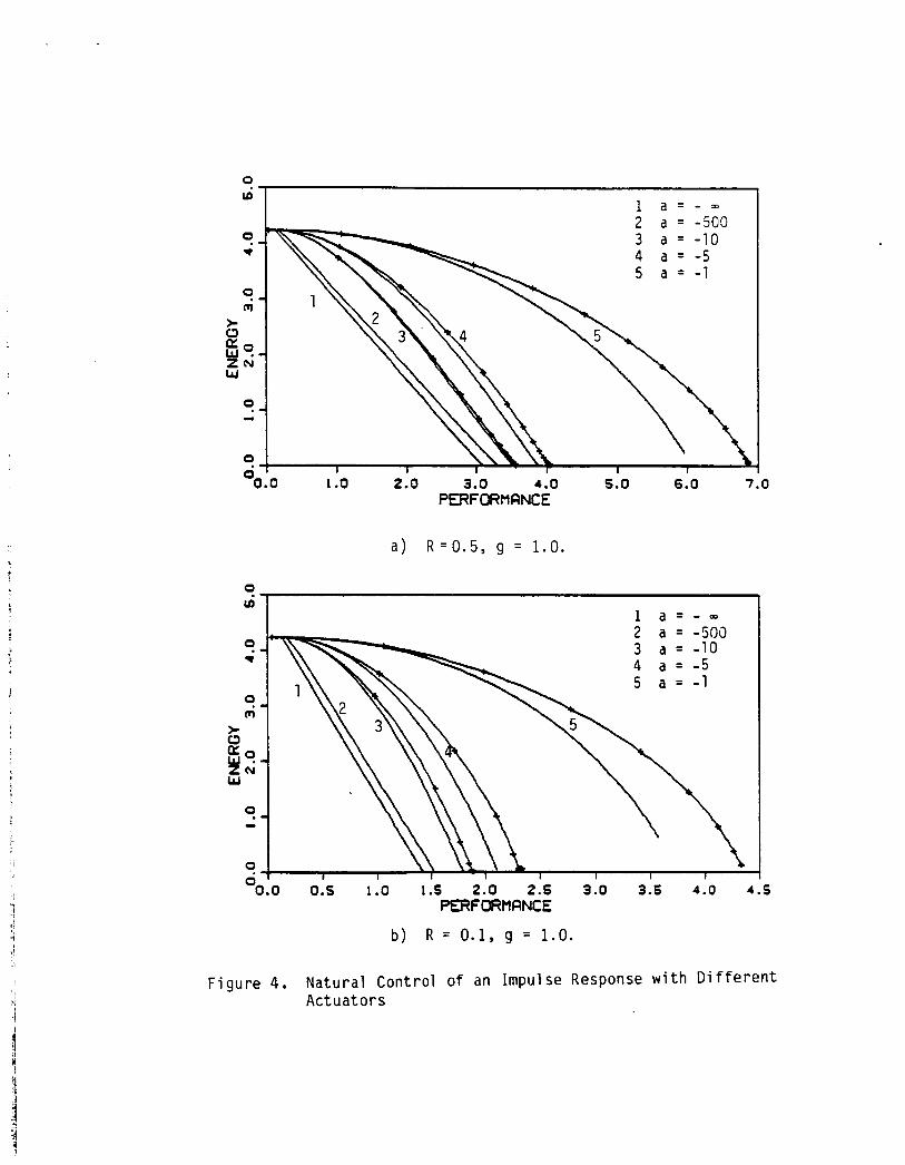
To illustrate the effects of the actuator dynamics, the model is

struck with an impulsive force of magnitude 5 lb in the yo direction.

The structure is initially in a state of rest. The ensuing motion is

modeled w i t h 15 modes and the first 10 modes are controlled with natural

control applied with distributed actuators and sensors. Both the

classical form of natural control and natural control adapted to include

the actuator dynamics is used to suppress the vibrations.

Figures 4a and 4b contain plots of the total energy of the system

versus the control performance for various values of the actuator

r e s p ~ n s e decay rate a. The values of R in the performance functional

are 0.5 and 0.1 for F igs . 4a and 4 b , respect ively, while q = 1 i n both

cases, f o r a l l modes. The symbol + s i g n i f i e s a solut ion w i t h c l a s s i c a l

natural control , i n which actuator dynamics i s not included. I n a l l

cases, the performance i s improved w i t h inclusion of actuator dynamics

i n the control formulation. Of course, as a + - = t h i s difference

approaches zero. Note t h a t , comparing F i g s . 4a and 4 b , t h i s d i f ference

also depends on the value of R. As R decreases, the modal decay r a t e

increases according t o Eq. (63) . Hence, the benef i t s derived from

including the actuator dynamics i n the control formulation depend on the

r a t i o of the desired modal decay r a t e t o the ac tua tors ' decay ra te . Of

course, as th i s r a t i o i s decreased, the e f f e c t of actuator dynamics

becomes l e s s important.

3a-c, a s imilar conclusion can be made about the e f f e c t of actuator

dynamics on the maneuver control . In this case, the r a t i o o f i n t e r e s t

is t h a t of the mean angular maneuver veloci ty t o the actuator decay

ra te .

As can be observed from a comparison of Figs .

The remainder of this section i s concerned w i t h the vibrat ion

control of the 30" and 180" r o l l maneuvers i n space. The f i r s t f i f t e e n

modes a re modeled f o r the simulations. Simulations a re presented

without vibrat ion controls i n Ref. 2, showing the exc i ta t ion of the

s t ruc ture by centr i fugal and tangent ia l forces .

Figure 5 i s a time-lapse p lo t of the spacecraf t d u r i n g the 30" r o l l

maneuver without vibrat ion control. The r o t a t i o n is produced by

actuators located on the s h u t t l e , so t h a t centr i fugal and tangent ia l

forces cause s t ruc tura l vibration.

s t ruc ture , showing the yozo plane w i t h the xo axis directed i n t o the

The view i s from d i r e c t l y behind t h e

----- p a p c i . n L A + -3-h EULII n l n + + ; n n ~ I U L L ' I I I Y camnlino ~ U V Q ~ S - S J t ime, t\;g plo t s appear, one i n dashed

l ines representing the s t ructure as i f i t were r i g i d and the other

representing the deformed s t ructure . As the s t r u c t u r e i s accelerated,

the appendage lags behind i t s desired posi t ion and then i t bounces

forward t o precede the desired configuration d u r i n g decelerat ion. When

the maneuver ends, the appendage continues t o v ibra te about the desired

target s t a t e .

The control techniques of Sec. 6 were applied t o control the

vibration o f the spacecraft d u r i n g the 30" r o l l . In a l l the presented

cases, R = 0.01 and q = 1.0 f o r a l l the control led modes. The time

constant of the ac tua tors ' equations of motion was assumed t o be a =

-10, as i n the maneuver strategy. Figure 6 i s a time-lapse p lo t of the

spacecraft d u r i n g the maneuver w i t h uniform damping control suppressing

the vibrations of the f i r s t 9 modes u s i n g the ten ac tua tors , six on the

s h u t t l e and four t h r u s t e r s , two a t the end of the mast and two a t the

antenna hub .

control d u r i n g the maneuver provides excel lent performance.

Comparing Figs. 5 and 6, we conclude t h a t uniform damping

The spacecraft was maneuvered through the 30" angle w i t h both

dis t r ibuted actuators and the 10 actuators discussed above. These 10

actuators were used f o r both maneuver control and vibrat ion suppression.

First, natural control approximated w i t h projected actuat ing and

dis t r ibuted sensing was used.

actuators and the maneuver was repeated u s i n g natural control

approximated by projected sens ng and actuat ing. F ina l ly , uniform

damping control was used w i t h he same 10 collocated ac tua tors and

sensors.

Next, 10 sensors were collocated w i t h the

Figures 7a and 7b show the t o t a l energy i n the system and the t o t a l

command e f f o r t versus time, r ~ s p s c i i v e l y , f o r a l l f o u r o f t h e abcve

mentioned control strategies. At the completion o f the maneuver, energy

is lower in all four strategies and the performance during the n 1 aneuver

is always better compared to the case of no vibration suppression shown

in Ref. 2. Distributed sensors and actuators yield the best performance

by far. Note that uniform damping control performs almost as well as

projected actuating and distributed sensing. This is to be expected, as

the former is an approximation o f the latter. However, it must be

recalled that uniform damping control is decentralized and requires only

a finite number of sensors, equal to the number of actuators.

The case o f projected actuating and sensing is clearly inferior to

uniform damping control, even though both techniques were applied with

the same collocated sensors and actuators. The difference lies in the

feedback method. Uniform damping control is decentralized, so that each

sensor supplies information only for the collocated actuator, requiring

no interpolation. On the other hand, the projected actuating and

sensing strategy is centralized so that the modal states are estimated

through interpolation o f signals from all the sensors. The actuators

are commanded from the estimated modal states. Hence, t o reduce modal

estimation error with projected sensing, more sensors are needed, as

discussed in Sec. 6 . Better modal filtering techniques can help to

reduce the modal estimation error, but in general, more sensors than

actuators are required.

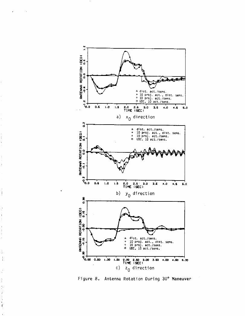
The main control objective of the SCOLE project is aiming the

antenna within a certain tolerance in minimum time. Hence, a study of

the antenna rotations versus time is of interest. Figures 8a-c

illustrate the instantaneous antenna rotations with respect to the frame

“yo’o about t h e x o, yo and ’0 axes, respectively; ?he p l o t s include

,

the responses produced during the maneuver with all four o f the Cbove

control implementation techniques. The relative quality of perfcrmance

is as mentioned above.

The effect of controlling only a finite set of modes is reflected

in Fig. 8b in the form of residual motion of the uncontrolled modes.

Uniform damping control dissipates energy in all of the modes, not just

a finite set. From Fig. 8b, however, we observe that it is not Lery

effective in controlling certain modes due to actuator placement.

Nevertheless, with time, it does remove all of the energy from the

system, unlike other implementation techniques.

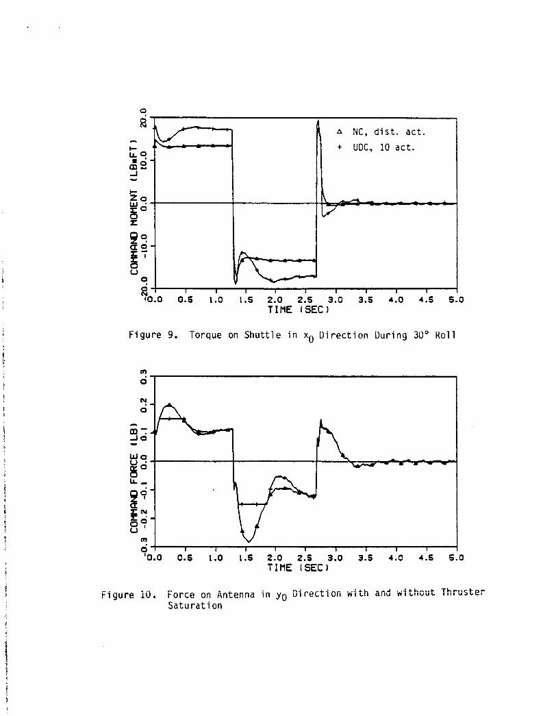
In reality, because of saturation, actuators can only produce a

finite amount of force or moment. The effect of limited command forces

was investigated for the 30" roll maneuver and uniform damping

control. The shuttle command forces and moments were limited to 2 lb

and 20 ft-lb, respectively. The four thrusters on the appendage were

each limited to 0.15 lb. These values correspond to saturation of the

thruster on the antenna hub in the yo direction.

plots o f this command force versus time for limited and unlimited

actuation. The corresponding plots of modal vibrational energy versus

time in Fig. lla show the adverse effect of command force truncation.

The price for force truncation is increased vibrational energy as well

as an associated increase in overall effort, as illustrated by F i g . lib,

although the control scheme is still effective.

Figure 10 contains

The maneuver and control techniques are now demonstrated for a more

extreme situation, a 180" roll maneuver with Mma, = 60 ft-lb. From Fig.

3c, we conclude that this i s a relatively severe maneuver in that a 180"

r o i l , starting and eiidSrig a t rest, takes place i!! less than 4 seconds.

A

Natural contro

press the vibration

and q = 1.0. First

and uniform damping

of the structure dur

natural control was

Attempting this maneuver with actuators located only on the shuttle and

without vibration controls resulted in deformations of the appendage

exceeding greatly the small elastic motions assumption.

control were employed tc sup-

ng the maneuver using R = -01

applied with distributed

actuators and sensors to establish a "best case". Uniform darnpino

control was then applied with the same 10 actuators and sensors used

previously. Finally, uniform damping control was used with two

additional thrusters (and collocated sensors), one in the zo direction

at the hub of the antenna and the other at the extreme tip of the

antenna in the yo direction.

The time-lapse plots of the structure during the maneuver showed no

discernible deformations for all three control techniques. Figures 12a

and 12b show the total modal energy and actual command effort versus

time, respectively, for three control implementation techniques. Figure

12c illustrates the antenna rotation about the xo direction for all

three cases. The addition of just two actuators resulted in much better

performance and a reduction in effort of approximately 50%.

maneuver and vibration control approach i s successful even in extreme

situations and the necessary number of actuators depends on the

performance requirements.

Hence, the

VIII. CONCLUSIONS

The perturbation method of s o l v i q the equations o f motion permits

the maneuver and vibration controls to be formulated independently.

This eliminates the numerical difficulties encountered Refs. 3-5 when

many modes are controlled. The quasi-modal equations o f motion permit

an efficient vibration simulation as well as a straightforward vibraticn

control formulation. Both uniform damping control and natural control

were found to be effective in controlling vibration even during

relatively quick maneuvers. The force distributions for both the

maneuver control and uniform damping control depend exclusively on the

mass matrix. Because the mass matrix is time invariant, these control

formulations are not affected during the maneuver and, hence, are

robust.

both for maneuver and vibration controls. Actuator dynamics causes a

time lag in force application, which degrades control performance.

Including the actuator dynamics along with the structure dynamics in the

control formulation minimizes this degradation.

The optimal actuator locations are the points of maximum mass

REFERENCES

1.

2.

3 .

4.

5.

6.

Meirovitch, L. and Quinn, R. D. "Equations of Motion for Maneuvering Flexible Spacecraft," Proceedings of the fifth VPI&SU/AIAA Symposium on Dynamics and Control of Larqe Structures, Blacksburg, Virginia, June 12-14, 1985.

Quinn, R. D. and Meirovitch, L., "Maneuver Control and Vibration Simulation of flexible Spacecraft," AIAA/ASME/ASCE/AHS 26th Structures, Structural Dynamics, and Materials Conference, San Antonio, Texas, May 19-21, 1986.

Turner, J. D. and Junkins, J . L., "Optimal Large-Angle Single-Axis Rotational Maneuvers of Flexible Spacecraft," Journal of Guidance and Control, Vol. 3, No. 6, 1980, pp. 578-585.

Turner, J. D. and Chun, H. M., "Optimal Distributed Control of a Flexible Spacecraft During a Large-Angle Maneuver," Journal o f Guidance, Control, and Dynamics, Vol. 7, No. 3, 1984, pp. 257-264.

Breakwell, J. A., "Optimal feedback Slewing of Flexible Spacecraft," Journal of Guidance and Control, Vol. 4, No. 5, 1981, pp. 372-479.

Baruh, H. and Silverberg, L., "Maneuver of Distributed Spacecraft," AIAA Guidance and Control Conference, Seattle, Washington, Aug. 20- 22, 1984.

7.

8.

9.

10.

11.

12.

13.

14.

15.

16.

Hale, A. L. an3 Rahn, G. A., "Robust Control of Self-Adjoint Distributed-Parameter Structures," Journal of Guidance, Control, a r d Dynamics, Vol. 7, No. 3, 1984, p p . 265-273. Meirovitch, L. and Baruh, H., "Control of Self-Adjoint Distributed- Partineter Systems,'' Journal of Guidance and Control, Vol . 5, No. 1, 1982, pp. 60-66.

Meirovitch, L. and Silverberg, L. M., "Globally Optimal Control of Self-Adjoint Distributed Systems," Optimal Control Applications an: Methods, Vol. 4, 1983, pp. 365-386.

Meirovitch, L. and Baruh, H., "On the Robustness of the Independent Modal-Space Control Method," Journal of Guidance, Control, and Dynamics, Vol. 6, No. 1, 1983, pp. 20-25.

Meirovitch L. and Silverberg, L., "Control o f Non-Self-Adjoint Distributed-Parameter Systems," Journal o f Optimization Theory and Applications, Vol. 47, No. 1, 1985.

Meirovitch, L., Computational Methods in Structural Dynamics, Sijthoff & Noordhoff Co., The Netherlands, 1980.

Kirk, D. E., Optimal Control Theory, Prentice-Hall, Inc., Englewood Cliffs, NJ, 1970.

Meirovitch, L., Baruh, H. and Oz, H., " A Comparison of Control Techniques for Large Flexible Systems," Journal o f Guidance, Control, and Dynamics, Vol. 6, No. 4, 1983, pg. 302.

Meirovitch, L. and Baruh, H., "On the Implementation of Modal Filters for Control of Structures,'' Journal of Guidance, Control, and Dynamics, Vol. 8, No. 6, 1985, pp. 707-716.

Silverberg, L., "Uniform Damping Control o f Spacecraft," Proceedings of the Fifth VPI&SU/AIAA Symposium on Dynamics and Control o f Large Structures, Blacksburg, Virginia, June 12-14, 1985.

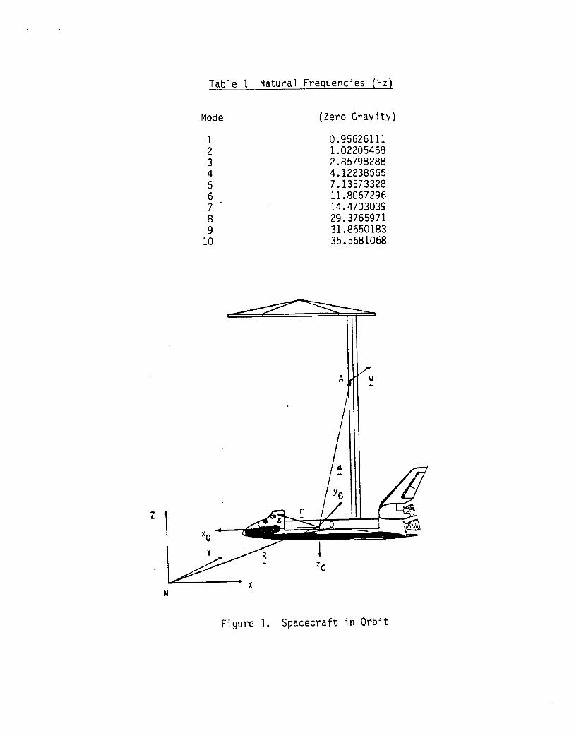
Tab le 1 Natural Frequencies (Hz)

Mode (Zero Gravity)

1 2 3 4 5 6 7 8 9

10

0.956261 11 1.02205468 2.85798288 4.12238565 7.13573328 11.8067296 14.4703039 29.3765971 31.8650183 35.5681068

U

Figure 1. Spacecraft in Orbit

i

,,,,,

13

F i gure 2. SCOLE Conf i gurat i on Showi ny Nodal Locat i ons

I

A rotation (rad) + ve 1 oci t y ' (rad/s ) o acceleration (rad/s 2 )

I I I I I I T i 0 0.s I .o 1 .s 2.0 2.5 3.0

TIRE I S E C I

a ) 30" r o l l , Mmax = 20 f t - l b .

9 ~ ~~~~~

w A ; veloc i ty rotation (rad/s) (rad) 2/

acceleration (rad/s ) * a 0 E: I

9 1 - 1 I I 1 I I

'0.0 1.0 2.0 3.0 4.0 5.0 6.0 7 .0 TIHE I S E C I

b ) 180" r o l l , Mmax = 20 f t - l b .

9 A rotation (rad) + veloc i ty (rad/s)

I-

- . '0.0 0.6 !.C 1.6 2.0 2.6 3.0 3.5 4.0

T I M I S E C I

c ) 180" r o l l , Mmax = 60 f t - l b .

F igu re 3. Comparison o f Maneuver S t ra teg ies

i

,

,I

' I ?! !

9 u)

9 t

9 (3

> 0

ZEV w 8 9

9

9 n Y

0.0 1 .o 2.0 3.0 4.0 s.0 6.0 7 . 0 PERFORflRNCE

a) R = O . 5 , g = 1.0.

9 t

9 m > 0

HK w

9

9 - ) - I I I

0.0 0.5 1.0 1.5 2.0 2.5 3.0 3.5 4.0 4.5 w

PERF ORflClNCE

R = 0.1, g = 1.0. b)

F i g u r e 4. Natura l Contro l o f an Impulse Response w i t h D i f f e r e n t Ac tua tors

I L aJ >

O n Ot- m o

I

,

c

I

I A

A d i s t . act./sens.

+ 10 p r o j . act , d i s t . sens. 0 10 p r o j . act./sens.

UnC, 10 act./sens

" m m 0"sa 1.00 1 . 5 0 2.00 2.90 3.00 3.50 4.00 4.50 5.00 TIME (SEGI

a ) Energy

u

A d i s t . act./sens.

+ 10 p r o j . act., d i s t . sens. 0 10 p r o j . act./sens.

9 2 UDC, 10 act./sens. /-- w g: =?

n

9 0.0 6.5 1.0 1.5 2.0 2.5 3.0 3.5 4.0 4.5 5.0

Q

TINE (SECl b) E f f o r t

F i g u r e 7. Comparison o f Various V i b r a t i o n Con t ro l Implementat ion Procedures f o r 30" R o l l Maneuver

1

n! - '0.0 0.5 1.0 1.S 2.0 2.5 3.0 3.S 4.0 4.5 5.0

TIME I S E C )

a ) xo d i r e c t i o n N 01 1

A dist. act./sens. + 10 p r o j . act., dist. sens. 0 I D p r o j . act./sens. 0 UDC, 10 act./sens.

'0 .0 0.6 1.0 1.6 2.0 2.5 3.0 7.5 4.0 4.S 5.0 TIRE I S E C )

b ) yo d i r e c t i o n SI 07 1

tC. n

d A

I I

7o:w 0:w *:oo 1:so zlw 2:so 31w 3:w 4roo *Is0 si, T t R E I S E C )

c ) zo d i r e c t i o n

F igu re 8. Antenna R o t a t i o n Dur ing 30" Maneuver

t

- c '

000- % ? - J -

+ UDC, 10 act .

\Y 10.0 0.5 1.0 1.S 2.0 2.5 3.0 3.5 4.0 4.5 5.0

TItlE ISEC)

c W 20

P 40 g2- is

S O

u 9

F i g u r e 9. Torque on S h u t t l e i n xo D i r e c t i o n Dur ing 30" Roll

? - 0

w o

0 I I I I I I I I I

'0.0 0.5 1.0 1.S 2.0 2.5 3.0 3.5 4.0 4.5 5.0 TItlE (SEC)

F i g u r e 10. Force on Antenna i n yo D i r e c t i o n w i t h and w i tho t i t Th rus te r S a t u r a t i o n

8- 0

A u n l i m i t e d forces

+ l i m i t e d forces 8- 0

W 0 - 2 0 W

00- Y O

8_; I I I I I I I I - I

0.00 0.50 1 . 0 0 1 . 5 0 2.00 2.w 3.00 3.50 4.00 4.50 5 0 -

+ l i m i t e d forces 8- 0

W 0 - 2 0 W

00- Y O

8_; I I I I I I I I - I

0.00 0.50 1 . 0 0 1 . 5 0 2.00 2.w 3.00 3.50 4.00 4.50 5.00 0 -

TIME ISEC) a

a) Energy

9 a A u n l i m i t e d forces

CL

N + l i m i t e d forces

m a

f

.OO

0 0

0 0.0 0.5 1.0 1.5 2.0 2.5 3.0 3.5 4.0 4.5 5.0

TIME ISECI b ) E f f o r t

X ? I " 0 0

? 0

0.0 0.5 1.0 1.5 2.0 2.5 3.0 3.5 4.0 4.5 5.0 TIME ISECI b ) E f f o r t

F i g u r e 11. E f f e c t s o f Actuator S a t u r a t i o n w i t h Uni form Damping Contro l Dur ing 30" Maneuver

A NC. d i s t . act . /sens.

~ 0 - + UDC, 12 act . /sens.

0 UDC, 10 act./sens.

-

TIRE ISEC) b ) Effort

0

c ) Antenna hub ro ta t ion in xo di rec t ion

Figure 12 . Implementation o f 180" Maneuver with Various Numbers of A c t u a t o r s