stat3014 { applied statistics

Semester 1, 2013 (Last adjustments: September 16, 2014)

Lecture Notes

STAT3014 – Applied Statistics

Lecturer

Dr. John T. Ormerod

School of Mathematics & Statistics F07

University of Sydney

(w) 02 9351 5883

(e) john.ormerod (at) sydney.edu.au

Binary Contingency Tables

We begin with a review of tests for 2-way contingency tables for two binary variables.

We will examine a variety of methods for analysing 2× 2 tables including:

2 Pearson’s χ2 statistic and the χ2 test for independence;

2 Odds ratios and relative risk, their relation to sampling methods and standard

errors for the log-odds ratio;

2 Fisher’s exact test; and

2 McNemar’s Test for 2× 2 Tables.

The first, third and fourth points are aimed at testing for independence, whereas

the second point is aimed at measuring the strength of a relationship between two

variables.

STAT3014: Week 1 2

Pearson’s Test for Independence

Suppose that R and S are both binary random variables and consider data

(R1, S1), . . . , (Rn, Sn).

The joint probability is

P (R = i, S = j) = pij, 1 ≤ i ≤ 2, 1 ≤ j ≤ 2.

Let xij be the observed count in the (i, j)th cell. We will use the • notation to

denote summation over a particular index. So that xi• is the sum of values in the

ith row and x•j is the sum of values in the jth column. Thus, we might present this

data as depicted in the table, often called a contingency table, below

S = 1 S = 2

R = 1 x11 x12 x1•R = 2 x21 x22 x2•

x•1 x•2 x•• = n

STAT3014: Week 1 3

Alternatively we use for 2 by 2 tables:

S = 1 S = 2

R = 1 a b a + b

R = 2 c d c + d

a + c b + d a + b + c + d = n

(but note that this notation doesn’t generalise to more complicated tables).

We will also use this convention for probabilities so that we may summarise the

probabilities as depicted below:

S = 1 S = 2

R = 1 p11 p12 p1•R = 2 p21 p22 p2•

p•1 p•2 p•• = 1

STAT3014: Week 1 4

Pearson’s χ2 Statistic

The most widely used statistic for testing structure in such tables is Pearson’s χ2

statistic:

X2 =

2∑i=1

2∑j=1

(observedi,j − expectedi,j)2

expectedi,j

where observedi,j = xij and the value of expectedi,j depends on the hypothesis at

hand. A simpler expression is: Pearson’s χ2 statistic:

X2 =

2∑i=1

2∑j=1

observed2i,jexpectedi,j

− n.which simplifies even further for 2 by 2 tables (Tutorial exercise) to

X2 =n(ad− bc)2

(a + b)(a + c)(b + d)(c + d)

STAT3014: Week 1 5

Pearson’s χ2 Statistic Distribution

This statistic, as the name might suggest, has an asymptotic χ21 distribution.

For more general tables Pearson’s χ2 statistic has a χ2k where the degrees of freedom

parameter k depends on the hypothesis at hand.

STAT3014: Week 1 6

Pearson’s χ2 Statistic – Justification

The null hypothesis for Pearson’s χ2 test for independence may be written as

H0 : pij = pi•p•j.

Under H0

pij = pi•p•j =xi•n× x•j

n.

Thus, the expected number of observations in the (i, j)th cell is

expectedi,j = npij =xi•x•jn

.

The fact that Pearson’s χ2 statistic has an asymptotic χ21 distribution result relies

on applying the Central Limit Theorem (CLT) and so it should be remembered that

the p-values calculated from the χ2 distribution are only approximations and they

become better approximations as n increases.

For this reason we should not use this test when the number of observations in a

cell is less than, say, 5.

STAT3014: Week 1 7

Peason’s χ2 Statistic – Justification

To get an intuitive feel for this link consider a simple test for proportions with

Z ∼ Binomial(n, p). Data might be presented by the following 1× 2 table:

Z = 1 Z = 0

x y

where we observe x successes and (n− x) = y failures.

Suppose that we wish to test the hypotheses

H0 : p = p0 vs Hi : p 6= p0.

For the above 1× 2 table Pearson’s χ2 statistic may be written as

X2 =

1∑i=0

(observedi − expectedi)2

expectedi=

(x− np0)2

np0+(y − n(1− p0))2

n(1− p0)

where under the null hypothesis expected1 = p0n, expected0 = (1 − p)0n, and

y = n− x.

STAT3014: Week 1 8

Under the CLT we have

p =Z

n

approx.∼ N

(p0,

p0(1− p0)n

).

Using this result we base the test on

|p− p0|√p0(1−p0)

n

∼ |N(0, 1)|

or, after squaring both sides,

n(p− p0)2

p0(1− p0)approx.∼ χ2

1.

STAT3014: Week 1 9

However,

n(p− p0)2

p0(1− p0)=

(x− np0)2

np0(1− p0)as p =

x

n

=(x− np0)2

np0+(x− np0)2

n(1− p0)

=(x− np0)2

np0+(y − n(1− p0))2

n(1− p0)as y = n− x.

Hence, since we know n(p− p0)2/(p0(1− p0)) is approximately χ21, we can deduce

that Pearson’s χ2 statistic is also approximately χ21.

Pearson’s χ2 statistic is important because, unlike some of the other tests we will

consider in this chapter, the ideas generalise to more elaborate contingency tables

than 2× 2 tables.

STAT3014: Week 1 10

Example

A hypothesis has been proposed that breast cancer in women is caused in part by

events that occur between the age at menarche (the age when menstruation begins)

and the age at first childbirth. An international study was conducted to test this hy-

pothesis. Breast cancer cases where identified amongst women in selected hospitals

in the US, Greece, Brazil, Taiwan and Japan. Controls were chosen from women of

comparable age who were in hospital at the sae time as the cases but who did not

have breast cancer. All women were asked of there aga at first birth and the results

were summarised in the table on the next slide.

In the table S = 1 if the age at first birth is greater than or equal to 30 and 2

otherwise and R = 1 for the cases and R = 2 for the controls.

STAT3014: Week 1 11

S = 1 S = 2

R = 1 683 2537 3220

R = 2 1498 8747 10245

2181 11284 13465

Under the assumption of independence the expected values (to 2 dp) are:

S = 1 S = 2

R = 1 521.56 2698.44

R = 2 1659.44 8585.56

X2 ≈ 6832

521.56+

25372

2698.44+

14982

1659.44+

87472

8585.56− 13465 ≈ 78.37

which is far too big when we compare it against a χ21 random variable. Hence, we

reject the null hypothesis for independence.

STAT3014: Week 1 12

Odds Ratios and Relative Risk

More often than not two way tables are generated by conditional sampling where

samples are drawn at each level of one factor and then these samples are classified

according to the observed values of the second factor.

For example, in a study of smoking (S) and lung cancer (R) data cannot be ob-

tained via a simple random sample from the complete population but we can obtain

information about the relationship via a prospective study where we take a large

sample of smokers and an independent sample of non-smokers and record these

people’s health status for several years to determine the proportion who develop

cancer. We can only estimate P (R = i|S = j) because the above method of col-

lecting the information does not allow us to estimate the proportion of smokers in

the population.

STAT3014: Week 1 13

Alternatively, we can use hospital records to construct a retrospective sample.

Under this scenario we draw samples from those known to have lung cancer and

those known to be free of lung cancer and classify people according to their smoking

history. This enables us to estimate P (S = j|R = i).

Regardless of how the data are collected they are presented as a contingency table.

It is critical that the person analysing the data understands how the data were

collected as this affects the interpretation of the statistical output. For Pearson’s χ2

test for independence the test statistic has an approximate χ21 distribution. However,

the conclusions drawn from the test depend on the sampling method used.

STAT3014: Week 1 14

Example

The table below is from New England Journal of Medicine, (1984) 318, 262–4.

Myocardial

Infarction

Yes No

Placebo 189 10,845 11,034

Aspirin 104 10,933 11,037

293 21,778 22,071

The data come from a 5 year (blind) study into the effect of taking aspirin every

second day on the incidence of heart attacks. The estimates for the proportion of

each subpopulation having heart attacks are

p1 =189

10, 845 + 189= 0.0171 estimating p1, say, and

p2 =104

10, 933 + 104= 0.0094 estimating p2, say.

STAT3014: Week 1 15

Relative Risk

The relative risk is the ratio of the outcome probabilities for the two groups, i.e.

p1/p2.

If we have

p1 =189


p2 =104

10, 933 + 104= 0.0094 estimating p2, say.

The estimated relative risk in the above case is 0.0171/0.0094 = 1.818.

We interpret this as saying that the sample proportion of heart attack cases for the

placebo group was 82% higher than that for the aspirin group. When the pi values

are small the relative risk or ratio is often of more interest than the absolute differ-

ence.

STAT3014: Week 1 16

Odds Ratios

Another common way of reporting the relationship in a 2× 2 table is via the odds

ratio or log-odds ratio.

The odds for group 1 is p1/(1− p1) and for group 2 is p2/(1− p2). The odds ratio

is

θ =odds 1

odds 2=p1(1− p2)p2(1− p1)

= Rel. Risk ×(1− p21− p1

)Note that if p1 = p2 then θ = 1. If θ > 1 then the odds of ‘success’ are higher in

group 1 than in group 2, and if θ < 1 then the reverse is true.

STAT3014: Week 1 17

Odds Ratios – Continued

If we have

p1 =189


p2 =104

10, 933 + 104= 0.0094 estimating p2, say.

In this example the odds for the placebo group is estimated to be

189/10845 = 0.0174,

i.e. 1.74 ‘yes’ cases for every 100 ‘no’ cases. The odds ratio is

(189/10845)/(104/10933) = 1.832

The estimated odds of heart attack for patients taking the placebo is 1.832 times

the estimated odds for those taking aspirin. The odds ratio (or log-odds ratio) is a

widely used measure of association as it can be estimated regardless of the sampling

scheme used to collect the data.

STAT3014: Week 1 18

For a completely random sample we can estimate pij = P (R = 1, S = j), with

i, j ∈ {1, 2} and hence estimate the odds ratio

p11/p12p21/p22

=p11p22p12p21

.

If we have conditional samples at each level of S, say, then we can estimate

P (R = i|S = j) =pij

p1j + p2j.

However, we cannot estimate pij itself because the number of subjects corresponding

the the category S is fixed. The odds ratio is given by

Odds ratio =P (R = 1|S = 1)/P (R = 2|S = 1)

P (R = 1|S = 2)/P (R = 2|S = 2)

=

p11p11 + p21

/ p21p11 + p21

p12p12 + p22

/ p22p12 + p22

=p11p22p12p21

=ad

bc.

STAT3014: Week 1 19

Standard Errors and Confidence Intervals

The odds ratio estimator θ has a skewed distribution on (0,∞), with the neutral

value being 1. The log odds estimator log(θ) has a more symmetric distribution

centred at 0 if there is no difference between the two groups.

[Note an odds ratio of a ∈ (0, 1) is equivalent to a value of a−1 ∈ (1,∞) just by

relabelling the categories. The log transformation is such that log(a−1) = − log(a).]

STAT3014: Week 1 20

Standard Errors and Confidence Intervals – Continued

The asymptotic standard error for log(θ) is√1

x11+

1

x21+

1

x12+

1

x22=

√1

a+1

b+1

c+

1

d

and a large sample confidence interval for log θ is approximately

log(θ)± zα/2√

1

x11+

1

x21+

1

x12+

1

x22= log(θ)± zα/2

√1

a+1

b+1

c+

1

d

from which we can approximate a confidence interval for the odds-ratio itself.

Note that these should only be applied if a, b, c and d are reasonably large (so that

aysmptotics hold).

STAT3014: Week 1 21

Example – Hodgkin’s Disease

The following data from Johnson & Johnson (1972) relate tonsillectomy and Hodgkin’s

disease.

Hodgkin’s No

Disease Disease

Tonsillectomy 90 165 255

No tonsillectomy 84 307 391

174 472 646

The data are from a case-control (retrospective) study.

We would like to know if tonsillectomy is related to Hodgkin’s disease. Pearson’s χ2

statistic is X2 = 14.96 and the p-value is P (χ21 > 14.96) = 0.0001. So we reject

the null hypothesis of independence and conclude that tonsillectomy is associated

with Hodgkin’s disease.

STAT3014: Week 1 22

(Note that this does not mean tonsillectomy causes Hodgkin’s disease. Suppose, for

example, that doctors gave tonsillectomies to the most seriously ill patients. The the

association between tonsillectomies and Hodgkin’s disease may be due to the fact

that those with tonsillectomies were the most ill patients and hence the more likely

to have a serious disease . We will pursue this issue later in the course).

The estimated odds-ratio and log odds-ratio are

Odds ratio =90× 307

165× 85= 1.99 and log( Odds ratio) = log(1.99) = 0.69

respectively. Hence, tonsillectomy patients are twice as likely to have Hodgkin’s

disease. The standard error of the log odds-ratio is√1

90+

1

84+

1

165+

1

307= 0.18.

A 95% confidence interval for the log odds-ratio is

0.69± 1.96× 0.18 ≈ (0.33, 1.05)

and a 95% confidence interval for the odds-ratio is (e0.33, e1.05) ≈ (1.39, 2.86).

STAT3014: Week 1 23

Fisher’s Exact Test

The χ2 approximation to the distribution of X2 and the deviance is only reasonable

when n is sufficiently large. Recall that we should only use the central limit theorem

based normal approximation to the binomial distribution, X ∼ Binomial(n, p) if

np ≥ 5 and n(1− p) ≥ 5.

The same rule of thumb can be applied to contingency tables.

The χ2 approximation is likely to be fine if the expected cell frequencies in the table

are all 5 or more. However, if this is not the case, then we need to take care and

maybe consider“exact” tests, i.e. calculating the exact p-value for the test statistic.

In R the function fisher.test() is available to carry out these calculations both

for 2× 2 tables and general contingency tables.

STAT3014: Week 1 24

The simplest exact test for contingency tables is Fisher’s test for 2 × 2 tables.

Consider the table:

A1 A2

B1 x11 x12 x1•B2 x21 x22 x2•

x•1 x•2 n

For a 2×2 table if we know the row and column and x11 then the table is completely

specified. A test of

H0 : θ = 1 (odds ratio = 1) vs HA : θ > 1

(or HA : θ < 1) can be based on the observed value of x11 given the marginal totals.

STAT3014: Week 1 25

If H0 is true and we know the x1•, x•1 and n values we expect x•1 × x1•n in the

(1, 1)th cell. To obtain the distribution of x11 given the marginal values note the

situation is like selecting x•1 values from n where x1• are type B1 and x2• are type

B2. Then

P (X11 = x11) =

(x1•x11

)(x2•

x•1 − x11

)(n

x•1

) ,

which is the hypergeometric distribution.

STAT3014: Week 1 26

P-values

To calculate the p-value for a particular table we need to:

2 Enumerate all tables, as extreme, or more extreme than the obsered table with

the same marginal totals.

2 Sum up the probability of each of these tables.

Note for a 2 by 2 table the probability an individual table (under H0 simplifies to:

P (a, b, c, d) =(a + b)!(c + d)!(a + c)!(b + d)!

n!a!b!c!d!

which can be useful when calculating these probabilities by hand.

STAT3014: Week 1 27

The Hypergeometric Distribution

The hypergeometric distribution relates to sampling without replacement from a

finite population. A population of size N is split into two types x1• of type 1, x2•of type 2. We draw a sample of size n = x•1. Let X denote the number of type 1

in the sample of size n then

P (X = x) = =

(x1•x

)(x2•

x•1 − x

)(N

x•1

) .

STAT3014: Week 1 28

Note that it can be shown that:

E(X) = x•1

(x1•N

)= x•1p

and

Var(X) = x•1p(1− p)(N − nN − 1

)where p is the proportion of type 1, i.e. x1•/N . Substituting this into the variance

formula we obtain:

Var(X) =x1• x2• x•1 x•2N 2(N − 1)

.

STAT3014: Week 1 29

Example

Mendenhall et al. (Int. J. Rad. Oncologist & Bio Phys, 10, 357-363 (1984)) reports

the results of a study comparing radiation therapy with surgery in treating cancer of

the larynx.

Cancer Cancer not

Controlled Controlled

Surgery 21 2 23

Radiation therapy 15 3 18

36 5 41

Suppose that we wish to test H0 : θ = 1 (both treatments equally effective) against

H1 : θ > 1 (surgery more effective).

STAT3014: Week 1 30

Example

First we need to enumerate all tables which are as extreme or more exteme than theobserved table. These are:

Cancer Cancer not


Surgery 21 2 23


36 5 41

Cancer Cancer not


Surgery 22 1 23


36 5 41

Cancer Cancer not


Surgery 23 0 23


36 5 41

STAT3014: Week 1 31

Let X be the number of surgery cases where cancer is controlled. Applying Fisher’s

approach

p-value = P (X ≥ 21| marginal totals)

= P (X = 21, 22, 23| marginal totals)

=

(23

21

)(18

15

)(41

36

) +

(23

22

)(18

14

)(41

36

) +

(23

23

)(18

13

)(41

36

)= 0.3808.

Extensions of this idea to higher order tables exist and are based on the multivariate

version of the hypergeometric distribution. However, the amount of calculations in-

volved means these techniques are rarely implemented without access to a computer.

STAT3014: Week 1 32

However, if we use Pearson’s χ2 test directly

X2 =41(3× 21− 2× 15)2

23× 18× 36× 5= 0.5992.

p-value ' P (χ21 ≥ 0.5992) = 0.4389.

STAT3014: Week 1 33

McNemar’s Test for 2× 2 Tables

McNemar’s test for 2 × 2 tables is a special test which applies to the special case

where the data relates to matched pairs of subjects. It is used to determine whether

the row and column marginal frequencies are equal (sometimes called “marginal

homogeneity”).

Second Survey

Yes No

First survey Yes a b

No c d

n

STAT3014: Week 1 34

Suppose n people are surveyed. Let (Xi, Yi) denote the responses of the ith person

to both surveysXi = 1 if ‘Yes’ at initial survey

= 0 if ‘No’

Yi = 1 if ‘Yes’ at second survey

= 0 if ‘No’.

Let Zi = Yi −Xi, p1 = E(Xi) and p2 = E(Yi). We are interested in testing

H0 : p1 = p2

against some alternative.

STAT3014: Week 1 35

McNemar’s Test for 2× 2 Tables – continued

We are interested in testing

H0 : p1 = p2

We base the test on the sample average difference between the Yis and the Xis,

Z =1

n

n∑i=1

(Yi −Xi) = p2 − p1

Under the null hypothesis

E(Z) = p2 − p1 = 0.

The Zi are independent so if n is large we can apply the CLT and base the test on

Z√Var(Z)

approx.∼ N(0, 1)

or equivalently

Z2

Var(Z)

approx.∼ χ2

1.

STAT3014: Week 1 36

Based on the table the value of Z is given by

Z =(a + c

n

)−(a + b

n

)=c− bn

.

Then Var(Z) is given by

Var(Z) =1

nVar(Z1)

=1

nE(Yi −Xi)

2

=1

n

[(1)2 × P (Y1 = 1, X1 = 0) + (−1)2P (Y1 = 0, X1 = 1) + 0

]=

1

nP (X1 6= Y1)

We can estimate P (X1 6= Y1) by

P (X1 6= Y1) =b + c

n

STAT3014: Week 1 37

which we use to obtain the test statistic,

T =(b− c)2

(b + c).

For a 2-sided test of H0 vs H1 : p1 6= p2 the p-value is approximately given by

p-value ' P(χ21 ≥ T

).

For a 1-sided test we need to use the normal version of the statistic.

STAT3014: Week 1 38

Example

Suppose that we want to compare two different chemotherapy regiments for breast

cancer after mastectomy. We assume that the two treatment groups are as com-

parable as possible along other prognostic factors. To accomplish this a matched

study is set up such that a random member of each matched pair gets treatment A

(chemotherapy) perioperatively (within 1 week after mastectomy) and for an addi-

tional 6 months, whereas the other members get treatment B (chemotherapy only

perioperatively).

The patients are assigned to pairs matched on age (within 5 years) and on clinical

condition. The patients are followed for 5 years with survival as the outcome variable.

Results are summarised on the next slide.

STAT3014: Week 1 39

Treatment B

Survive Die

Treatment A Survive 510 16

Die 5 90

n

T =(16− 5)2

(16 + 5)= 5.761905

which, when compared to a χ21 distribution gives a p-value of 0.0163. Thus we reject

the null that row and column marginal frequencies are equal and conclude that there

is evidence of a difference in outcome between treatment A and B.

STAT3014: Week 1 40

General 2-way Contingency Tables

We now turn our attention from 2× 2 table to r × s tables with classifying factors

R at r levels and S at s levels. Let

P (R = i, S = j) = pij, 1 ≤ i ≤ r, 1 ≤ j ≤ s.

Let xij be the observed count in the (i, j)th cell. Again, we will use the • notation

to denote summation over a particular index. So that xi• is the sum of values in the

ith row and x•j is the sum of values in the jth column.

STAT3014: Week 1 41

Thus, we might present this data as depicted in the table, often called a contingency

table, below

S = 1 · · · S = s

R = 1 x11 · · · x1s x1•... ... . . . ... ...

R = r xr1 · · · xrs xr•x•1 · · · x•s x••

Hence, x•• =∑r

i=1

∑sj=1 xij = n, the sample size.

STAT3014: Week 1 42

We will also use this convention for probabilities so that we may summarise the

probabilities as depicted below:

S = 1 · · · S = s

R = 1 p11 · · · p1s p1•... ... . . . ... ...

R = r pr1 · · · prs pr•p•1 · · · p•s 1

STAT3014: Week 1 43

The most widely used statistic for testing structure in such tables is Pearson’s χ2

statistic:

X2 =

r∑i=1

s∑j=1

(observedi,j − expectedi,j)2

expectedi,j

where observedi,j = xij and the value of expectedi,j depends on the hypothesis at

hand.

This statistic, as the name might suggest, has an asymptotic χ2k distribution. The

degrees of freedom parameter k also depends on the hypothesis at hand.

The χ2 result relies on applying the Central Limit Theorem (CLT) and so it should

be remembered that the p-values calculated from the χ2 distribution are only ap-

proximations and they become better approximations as n increases.

STAT3014: Week 1 44

Pearson’s χ2 Test of Independence for General 2-Way Tables

Suppose we have a completely random sample of size n classified by R and S. We

want to test

H0 : R and S are independent.

When R and S are independent we will use the notation R⊗ S.

If R⊗ S then, be definition of independence,

pij = P (R = i, S = j) = P (R = i)P (S = j)

STAT3014: Week 1 45

If R⊗ S then, be definition of independence,

pij = P (R = i, S = j) = P (R = i)P (S = j)

This equation allows us to estimate the marginal probabilities P (R = i) and P (S =

j) via

P (R = i) = pi• =

s∑j=1

pij estimated by(∑s

j=1 xij)

n=xi•n

and

P (S = j) = pj• =

r∑i=1

pij estimated by(∑r

i=1 xij)

n=x•jn.

Hence, under the independence hypothesis, the expected frequency in the (i, j)th

cell is

expectedi,j = npij = npi•p•j =xi•x•jn

STAT3014: Week 1 46

Pearson’s χ2 statistic is then given by

X2 =

r∑i=1

s∑j=1

(xij −xi•x•jn )2

(xi•x•jn )

which, after using the fact that∑r

i=1

∑sj=1 xij = n, may be written as

X2 =

r∑i=1

s∑j=1

(x2ijn

xi•x•j

)− n.

Under the null hypothesis Pearson’s χ2 statistic is asymptotically

X2 approx.∼ χ2

(r−1)(s−1).

Again, this test should only really be applied when all cells have counts greater than

5. Otherwise the R comment fisher.test() should be used.

STAT3014: Week 1 47

Contingency Table Example 1

The below table refers to a study that assessed factors associated with women’s

attitudes toward mammography (Hosmer & Lemeshow, 1989). The below table

gives the responses to the question ‘How likely is it that a mammogram could find

a new case of breast cancer?’

Mammography Detection of breast cancer

experience Not likely Somewhat likely very likely

Never 13 77 144

Over one year ago 4 16 54

Within the past year 1 12 91

STAT3014: Week 1 48

The R output follows.

> a = c(13, 77, 144, 4, 16, 54, 1, 12, 91)

> am = matrix(a, ncol = 3, byrow = T)

> am

[,1] [,2] [,3]

[1,] 13 77 144

[2,] 4 16 54

[3,] 1 12 91

> chisq.test(am)

Pearson's Chi-squared test

data: am

X-squared = 24.1481, df = 4, p-value = 7.46e-05

STAT3014: Week 1 49

> rp = apply(am, 1, sum)/sum(am)

> rp

[1] 0.5679612 0.1796117 0.2524272

> cp = apply(am, 2, sum)/sum(am)

> cp

[1] 0.04368932 0.25485437 0.70145631

> exp = rp %*% t(cp) * sum(am)

> exp

[,1] [,2] [,3]

[1,] 10.223301 59.63592 164.14078

[2,] 3.233010 18.85922 51.90777

[3,] 4.543689 26.50485 72.95146

STAT3014: Week 1 50

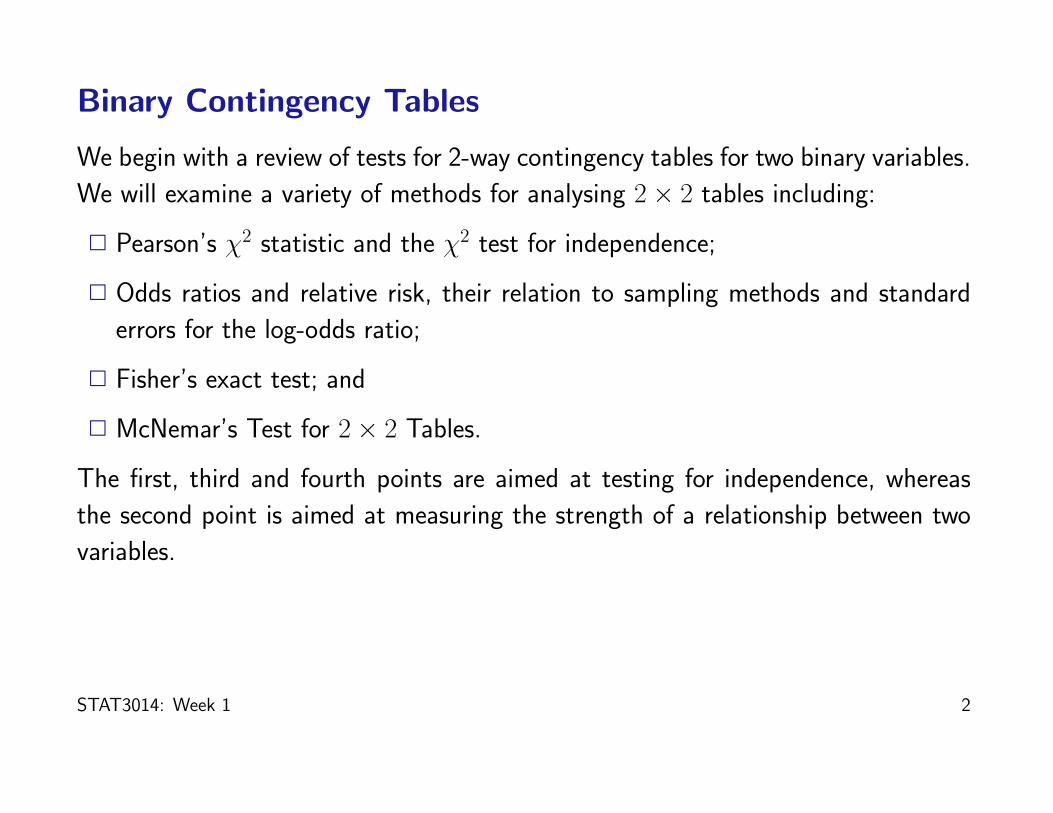
> obs = am

> mat = (obs - exp)^2/exp

> mat

[,1] [,2] [,3]

[1,] 0.7541652 5.0558654 2.4713596

[2,] 0.1819587 0.4334833 0.0843311

[3,] 2.7637748 7.9378214 4.4652971

> chisqstat = sum(mat)

> chisqstat

[1] 24.14806

> 1 - pchisq(chisqstat, df = 4)

[1] 7.459772e-05

STAT3014: Week 1 51

Given two of the entries are less than 5 in the first column we cound try to combine

the first and second columns.

> bm = cbind(am[, 1] + am[, 2], am[, 3])

> bm

[,1] [,2]

[1,] 90 144

[2,] 20 54

[3,] 13 91

> chisq.test(bm)


data: bm


Thus there is strong evidence that the person’s response varies with the recentness

of their mammography experience.

STAT3014: Week 1 52

Contingency Table Example 2

The following data from Norton and Dunn (Brit. Med. J. 291 (1985), 630-632)

relates to an epidemiological survey of 2484 subjects to investigate snoring as a

possible risk factor for heart disease. Those surveyed were classified according to

their partner’s report of how much they snored. The data are:

Heart disease

Snoring Yes No

Never 24 1355

Occasional 35 603

Nearly every night 21 192

Every night 30 224

STAT3014: Week 1 53

(a) Is the risk of a heart attack independent of snoring frequency?

> a <- c(24, 1355, 35, 603, 21, 192, 30, 224)

> am <- matrix(a, ncol = 2, byrow = T)

> am

[,1] [,2]

[1,] 24 1355

[2,] 35 603

[3,] 21 192

[4,] 30 224

> chisq.test(am)


data: am


STAT3014: Week 1 54

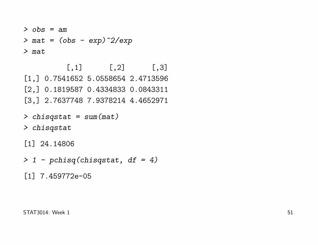
(b) For each cell calculate the expected frequency under the independence model.

Calculate the Pearson residuals

rij =oij − eij√

eij.

Note that Pearson’s statistic is just the sum of the squares of these values. The

expected frequencies under the independence model are:

> r <- apply(am, 1, sum)

> r

[1] 1379 638 213 254

> c <- apply(am, 2, sum)

> c

[1] 110 2374

> r <- matrix(r, ncol = 1)

> c <- matrix(c, ncol = 1)

STAT3014: Week 1 55

> sum(am)

[1] 2484

> ex <- r %*% t(c)/sum(am)

> ex

[,1] [,2]

[1,] 61.066828 1317.9332

[2,] 28.252818 609.7472

[3,] 9.432367 203.5676

[4,] 11.247987 242.7520

STAT3014: Week 1 56

The Pearson residuals are:

> res <- (am - ex)/sqrt(ex)

> res

[,1] [,2]

[1,] -4.743323 1.0210305

[2,] 1.269380 -0.2732420

[3,] 3.766467 -0.8107559

[4,] 5.591270 -1.2035565

> sum(res^2)

[1] 72.78206

If we focus on the first column we notice that the residuals are strictly increasing

(or strictly decreasing if we look at column 2).

STAT3014: Week 1 57

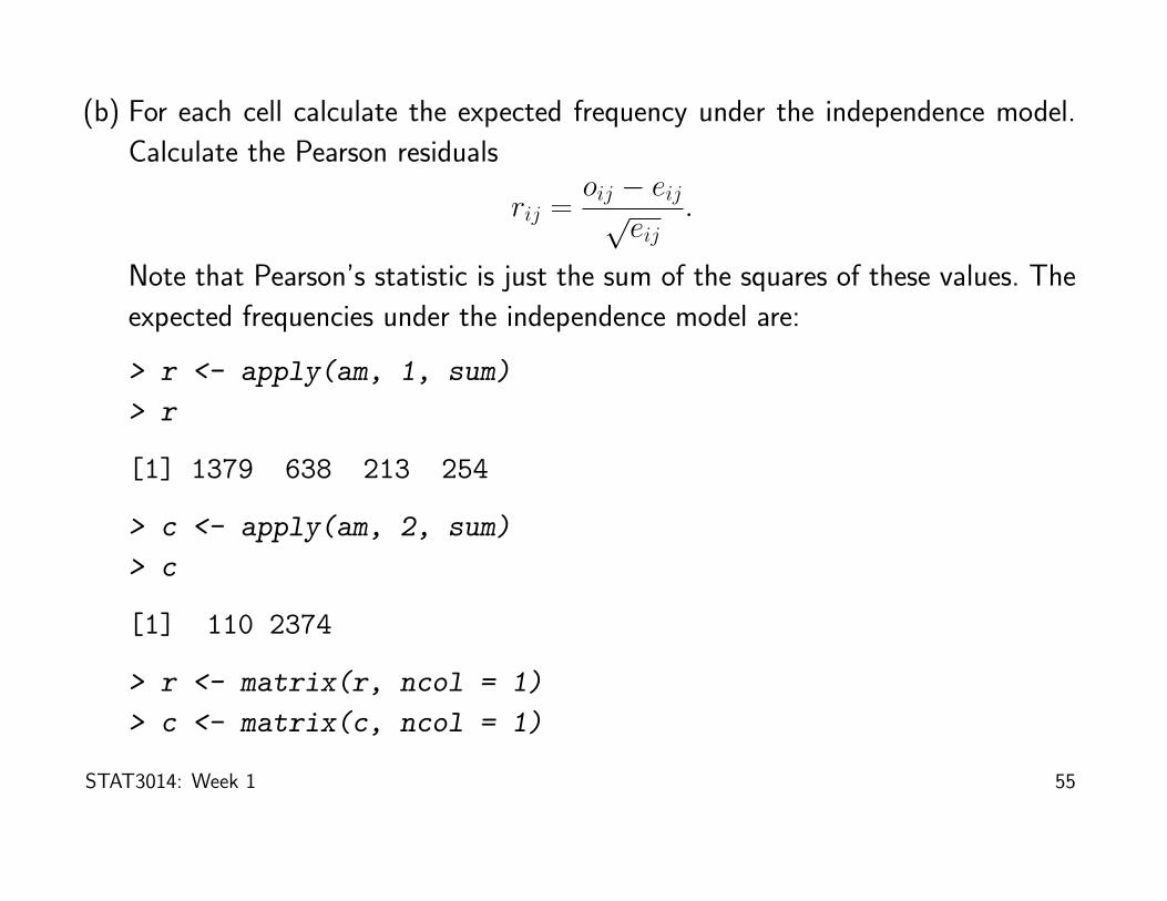
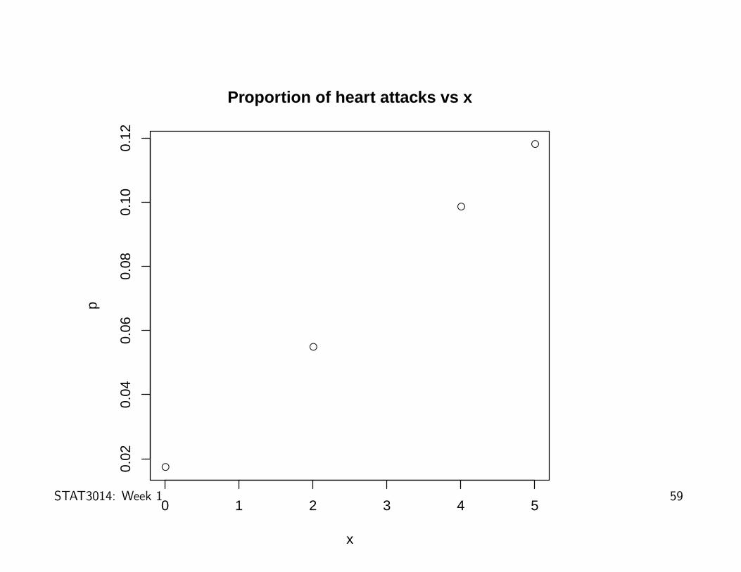
(c) The investigator gives the 4 snoring categories an x score of 0, 2, 4 or 5 going

from ‘never snores’ to ‘snores every night’. Plot the estimated probability of heart

attack against x.

> x <- c(0, 2, 4, 5)

> p <- am[, 1]/(am[, 1] + am[, 2])

> p

[1] 0.01740392 0.05485893 0.09859155 0.11811024

> plot(x, p, main = "Proportion of heart attacks vs x")

We can see from the next plot that the observed proportion of people suffering

a heart attack increases with x.

STAT3014: Week 1 58

●

●

●

●

0 1 2 3 4 5

0.02

0.04

0.06

0.08

0.10

0.12

Proportion of heart attacks vs x

x

p

STAT3014: Week 1 59

STAT3014: Week 1 60

(d) A model that relates the probability of a heart attack, p, to the snoring index, x

is

log

(p

1− p

)= −3.87 + 0.4x.

We can use the above model to calculate the probabilities of a heart attack for

each of the 4 groups.

> b = -3.87 + 0.4 * x

> b

[1] -3.87 -3.07 -2.27 -1.87

> p1 = exp(b)/(1 + exp(b))

> p1

[1] 0.02043219 0.04436183 0.09363821 0.13354172

STAT3014: Week 1 61

The expected frequencies for each of the cells in the contingency table.

> exp1 = p1 * r

> exp2 = (1 - p1) * r

> ex2 = cbind(exp1, exp2)

> ex2

[,1] [,2]

[1,] 28.17599 1350.8240

[2,] 28.30285 609.6972

[3,] 19.94494 193.0551

[4,] 33.91960 220.0804

Note there is reasonable agreement between p1 and p in (c).

STAT3014: Week 1 62

Thus, using Pearson’s X2 statistic to assess the fit of the model, we get:

> x2 = sum((am - ex2)^2/ex2)

> x2

[1] 2.874429

> 1 - pchisq(x2, 3)

[1] 0.4113937

Thus the model gives very good fit.

STAT3014: Week 1 63

Log-linear Models for 2-way Tables

Consider an r × s contingency table. If we have a completely random sample then

the joint distribution of the rs cell frequencies is multinomial. Let

pij = P (R = i, S = j), i = 1, . . . r; j = 1, . . . s.

We can analyse the data by assuming that the frequency in the (i, j)th cell is an

observation from a Poisson random variable,

Zij ∼ Poisson(npij)

with the Zijs independent. Given∑i

∑j

Zij = n,

the conditional distribution of the Zijs is multinomial. We can attempt to model

the structure in the pijs by using ANOVA type log-linear models.

STAT3014: Week 1 64

The model

Consider the model:

log pij = µ + αi + βj + λij,

with α1 = β1 = 0 and λ1j = λi1 = 0, i = 1, . . . , r, j = 1, . . . , s. It is easy to show

that the above constraints lead to

λij = log

(pijp11pi1p1j

).

Thus, λij is the log-odds ratio for the 2×2 table focussing on R = 1, i and S = 1, j.

The model with all λij set to 0 is the model of independence, that is, R and S are

independent if and only if λij = 0 for all i, j. Thus, we can check if the independence

model is reasonable by fitting the log-linear model with only main effects and using

the deviance as the test statistic. In this case the deviance has (r−1)(s−1) degrees

of freedom as we fit µ, (r − 1) different αi values and (s − 1) different βj values,

i.e. r + s− 1 parameters.

STAT3014: Week 1 65

Conditional Sampling

If the contingency table is constructed by sampling at each level of S, say, and then

classifying the response according to the value for R, we have information that allows

us to estimate the conditional probability P (R = i|S = j) but not P (R = 1, S = j)

as we have no information on the marginal distribution of S.

This structure is often referred to as the product multinomial model as the

likelihood can be thought of as the product of s multinomial distributions, one for

each level of S.

STAT3014: Week 1 66

In these situations we can also develop log-linear models.

logP (R = i|S = j) = µ + αi + βj + λij,

with α1 = β1 = 0 and λ1j = λi1 = 0, i = 1, . . . , r, j = 1, . . . , s.Here

λij = log

(P (R = i|S = j)P (R = 1|S = 1)

P (R = i|S = 1)P (R = 1|S = j)

).

If we have a constant probability distribution across levels of S then

P (R = i|S = j) = P (R = i|S = 1), i = 1, . . . , r; j = 1, . . . , s.

Clearly λij = 0 for all i and j in this case. The model with no interaction terms can

be interpreted as a model for homogeneity of proportions across levels of S.

STAT3014: Week 1 67

Theorem: λij = 0 if and only if P (R, S) = P (R)P (S)

To prove if and only if statements first we need to show one side of the if statement

to prove the other side, and then use the other side of the if statement to prove

the first side. To prove the first side. Assume that R and S are independent, i.e.,

P (R, S) = P (R)P (S). Now note that

λij = log

(pijp11pi1p1j

).

If P (R, S) = P (R)P (S) then pij = pi•p•j. Hence,

pij = pi•p•j,

p11 = p1•p•1 and

pi1 = pi•p•1,

p1j = p1•p•j.

Plugging these expressions into the expression for λij we get

λij = log

(pi•p•jp1•p•1pi•p•1p1•p•j

)= log(1) = 0

via cancellation.

STAT3014: Week 1 68

Now assume that the reverse is true, i.e. suppose that λij = 0 and so by assumption

pij = exp [µ + αi + βj] .

Then we want to show that pij = pi•p•j. Now

pi• = exp [µ + αi]∑j

exp [βj] ,

p•j = exp [βj]∑j

exp [µ + αi]

and

pi•p•j = exp [µ + αi + βj]∑i,j

exp [µ + αi + βj] = pij∑i,j

pij = pij

since (∑

i,j pij) = 1.

STAT3014: Week 1 69

Deviance for Log-linear Models in the Poisson case

To derive the deviance for a GLM we compare the log-likelihood under perfect fit with

the log likelihood maximised over the parameters in the current model. If z1, . . . , znare observations from Poisson populations, Zi ∼ Poisson(λi) then the likelihood is

n∏i=1

e−λiλzii /zi! = e−∑λi

n∏i=1

(λzii )/zi!.

The log-likelihood is

` = −n∑i=1

λi +

n∑i=1

zi log(λi)−n∑i=1

log(zi!).

STAT3014: Week 1 70

Under perfect fit (i.e. observed = expected) we have zi = λi so that

L1 = −n∑i=1

zi +

n∑i=1

zi log(zi)−n∑i=1

log(zi!),

whereas under the fitted model we get

L2 = −n∑i=1

λi +

n∑i=1

zi log(λi)−n∑i=1

log(zi!),

where λi is the expected value of Zi under the fitted model.

The (scaled deviance) is given by:

Deviance = D = 2(L1 − L2) = 2

n∑i=1

zi log(zi/λi) +

n∑i=1

(λi − zi).

(Note that the scaled deviance is the deviance for the Poisson case since α(φ) = 1).

STAT3014: Week 1 71

Deviance for Log-linear Models in the Poisson case

The deviance for Poisson models is given by:

Deviance = 2

n∑i=1

zi log(zi/λi) +

n∑i=1

(λi − zi).

For log-linear models with a constant term, i.e. µ,

∂L

∂µ= −

n∑i=1

λi +

n∑i=1

zi.

Setting the above to zero, for the Poisson case, the deviance becomes

D = 2

n∑i=1

zi log(zi/λi).

We can then use this statistic to test for independence. To do so we (i) Fit the

log-linear model without the interaction term and (ii) Use the deviance to test for

adequacy of fit.

STAT3014: Week 1 72

Relationship between Deviance and Pearson’s tests

From the previous slide the deviance simplified to

D = 2

n∑i=1

zi log(zi/λi).

The deviance for the Poisson model is closely related to Pearson’s χ2 statistic. To

see this consider the Taylor series expansion for f (z) = z log(z/a),

f (z) = f (a) + (z − a)f ′(a) + 1

2(z − a)2f ′′(a) +R,

where R is a remainder term. Hence,

f (z) = (z − a) + 1

2(z − a)2/a +R

and R = (z − a)3f (3)(ξ)/6, where ξ lies between z and a.

STAT3014: Week 1 73

Applying this result with a = λi we get

D = 2

n∑i=1

zi log(zi/λi)

≈ 2

n∑i=1

[(zi − λi) +

1

2(zi − λi)2/λi +Ri

]=

n∑i=1

(zi − λi)2

λi+ 2

n∑i=1

Ri

= X2 + a remainder term.

We can show that the remainder is typically very small when n becomes sufficiently

large. In fact the remainder goes to 0 with probability 1 as n→∞. For large n, D

and X2 should give similar values. Both statistics have an asymptotic χ2 distribution.

STAT3014: Week 1 74

Log-linear model: Example 1

In a study of children aged 0 to 15 years the following table was obtained (Armitage,

Biometrics 11 (1955), 375-386.)

Tonsils Tonsils Tonsils

not enlarged slightly enlarged very enlarged

Carriers 19 29 24

Non-carriers 497 560 269

STAT3014: Week 1 75

> y = c(19, 29, 24, 497, 560, 269)

> car = factor(c(1, 1, 1, 2, 2, 2))

> size = factor(c(1, 2, 3, 1, 2, 3))

> cbind(y, car, size)

y car size

[1,] 19 1 1

[2,] 29 1 2

[3,] 24 1 3

[4,] 497 2 1

[5,] 560 2 2

[6,] 269 2 3

> logl1 = glm(y ~ car + size, family = poisson)

> summary(logl1)

STAT3014: Week 1 76

Call:

glm(formula = y ~ car + size, family = poisson)

Deviance Residuals:

1 2 3 4 5 6

-1.54914 -0.24416 2.11019 0.34153 0.05645 -0.53736

Coefficients:

Estimate Std. Error z value Pr(>|z|)

(Intercept) 3.27997 0.12293 26.682 < 2e-16 ***

car2 2.91326 0.12101 24.075 < 2e-16 ***

size2 0.13232 0.06030 2.194 0.0282 *

size3 -0.56593 0.07315 -7.737 1.02e-14 ***

---

Signif. codes: 0 '***' 0.001 '**' 0.01 '*' 0.05 '.' 0.1 ' ' 1

(Dispersion parameter for poisson family taken to be 1)

Null deviance: 1487.217 on 5 degrees of freedom

Residual deviance: 7.321 on 2 degrees of freedom

AIC: 53.992

Number of Fisher Scoring iterations: 4

STAT3014: Week 1 77

> logl1$fitted

1 2 3 4 5 6

26.57511 30.33476 15.09013 489.42489 558.66524 277.90987

> deviance(logl1)

[1] 7.320928

> ym = matrix(y, ncol = 3, byrow = TRUE)

> chisq.test(ym)


data: ym

X-squared = 7.8848, df = 2, p-value = 0.0194

STAT3014: Week 1 78

> a = logl1$fitted

> x2 = sum((a - y)^2/a)

> x2

[1] 7.884843

Note that the fitted values from the log-linear fit are the same as those from the

homogeneous proportion model. The Residual deviance (7.32) is slightly less than

Pearson’s statistic (7.88) in this case. Both have 2 degrees of freedom.

STAT3014: Week 1 79

Log-Linear Example 2

An experiment on 75 rockets yields the characteristics of lateral deflection and range

as follows:

Lateral deflection

Range (m) -250 to -51 -50 to 49 50 to 199

0 - 1199 5 9 7

1200 - 1799 7 3 9

1800 - 2699 8 21 6

Are range and lateral deflection independent characteristics?

STAT3014: Week 1 80

> y = c(5, 9, 7, 7, 3, 9, 8, 21, 6)

> ym = matrix(y, ncol = 3, byrow = T)

> ym

[,1] [,2] [,3]

[1,] 5 9 7

[2,] 7 3 9

[3,] 8 21 6

> chisq.test(ym)


data: ym

X-squared = 10.4662, df = 4, p-value = 0.03327

STAT3014: Week 1 81

> r = factor(c(1, 1, 1, 2, 2, 2, 3, 3, 3))

> l = factor(c(1, 2, 3, 1, 2, 3, 1, 2, 3))

> glm2 = glm(y ~ r + l, family = poisson)

> summary(glm2)

Call:

glm(formula = y ~ r + l, family = poisson)

Deviance Residuals:

1 2 3 4 5 6 7 8

-0.2583 -0.0793 0.3312 0.8115 -2.1380 1.3315 -0.4475 1.3515

9

-1.4449

STAT3014: Week 1 82

Coefficients:

Estimate Std. Error z value Pr(>|z|)

(Intercept) 1.72277 0.29032 5.934 2.96e-09 ***

r2 -0.10008 0.31662 -0.316 0.7519

r3 0.51083 0.27603 1.851 0.0642 .

l2 0.50078 0.28338 1.767 0.0772 .

l3 0.09531 0.30896 0.308 0.7577

---

Signif. codes: 0 '***' 0.001 '**' 0.01 '*' 0.05 '.' 0.1 ' ' 1

(Dispersion parameter for poisson family taken to be 1)

Null deviance: 20.874 on 8 degrees of freedom

Residual deviance: 11.299 on 4 degrees of freedom

AIC: 55.98

Number of Fisher Scoring iterations: 5

STAT3014: Week 1 83

> glm2$fitted

> glm2$fitted

1 2 3 4 5 6 7 8

5.600000 9.240000 6.160000 5.066667 8.360000 5.573333 9.333333 15.400000

9

10.266667

STAT3014: Week 1 84

stat3014 { applied statistics

Documents