stat 302 - university of british columbiaruben/stat302website/lecture12.pdf · stat 302 ruben zamar...
TRANSCRIPT
Stat 302
Ruben [email protected]
Asymptotic Results
Ruben Zamar [email protected] () Module 12 Asymptotic Results 1 / 60

Motivation
Suppose we are interested on the overall performance of UBCstudents in the Stat 302 Final Exam.
Some questions we may have are:
What is the mean performance across all UBC students?Do women do better than men on average?Do CPSC students do better than other FOSC students?How likely is for a student to fail this test? Does this prob changeacross disciplines?
Ruben Zamar [email protected] () Module 12 Asymptotic Results 2 / 60

Motivation
Suppose we are interested on the overall performance of UBCstudents in the Stat 302 Final Exam.
Some questions we may have are:
What is the mean performance across all UBC students?
Do women do better than men on average?Do CPSC students do better than other FOSC students?How likely is for a student to fail this test? Does this prob changeacross disciplines?
Ruben Zamar [email protected] () Module 12 Asymptotic Results 2 / 60

Motivation
Suppose we are interested on the overall performance of UBCstudents in the Stat 302 Final Exam.
Some questions we may have are:
What is the mean performance across all UBC students?Do women do better than men on average?
Do CPSC students do better than other FOSC students?How likely is for a student to fail this test? Does this prob changeacross disciplines?
Ruben Zamar [email protected] () Module 12 Asymptotic Results 2 / 60

Motivation
Suppose we are interested on the overall performance of UBCstudents in the Stat 302 Final Exam.
Some questions we may have are:
What is the mean performance across all UBC students?Do women do better than men on average?Do CPSC students do better than other FOSC students?
How likely is for a student to fail this test? Does this prob changeacross disciplines?
Ruben Zamar [email protected] () Module 12 Asymptotic Results 2 / 60

Motivation
Suppose we are interested on the overall performance of UBCstudents in the Stat 302 Final Exam.
Some questions we may have are:
What is the mean performance across all UBC students?Do women do better than men on average?Do CPSC students do better than other FOSC students?How likely is for a student to fail this test? Does this prob changeacross disciplines?
Ruben Zamar [email protected] () Module 12 Asymptotic Results 2 / 60

Motivation (Continued)
Suppose we measure the independent performances of n = 65students (e.g. in April 12...).
The student’s performances Xi could be model as iid rv’s with(unknown) mean µ and variance σ2.
A quantity of possible interest is
P (|X − µ| < 5) =?
If this probability is large then we are confident that X estimates µwithin a 5 points error margin
Ruben Zamar [email protected] () Module 12 Asymptotic Results 3 / 60

Confidence Intervals
Other examples of quantities of possible interest are
P (L (X1, ...,Xn) < µ < U (X1, ...,Xn)) = 0.95?where L (X1, ...,Xn) and U (X1, ...,Xn) are some functions (calledestimates) that only depend on the data
P (L (X1, ...,Xn) < µW − µM < U (X1, ...,Xn)) = 0.95?
Unfortunately we cannot compute these probabilities exactly becausewe don’t know the actual distribution of the Xi .
Even if we knew the cdf of Xi , it may be inconvenient or unfeasible tocalculate the exact probabilities when L (X1, ...,Xn) andU (X1, ...,Xn) are complicated (non-linear) functions.
Ruben Zamar [email protected] () Module 12 Asymptotic Results 4 / 60

Asymptotic Approximation
We will learn in this course how to approximate these quantities whenn is “large”
These approximations are called “asymptotic calculations”
They are obtained by taking limit for n→ ∞The limiting results often give good approximation for moderatevalues of n (e.g. n = 20)
We will see that the standard normal cdf Φ (z) is a main tool forasymptotic calculations
Ruben Zamar [email protected] () Module 12 Asymptotic Results 5 / 60

Asymptotic Approximation
We will learn in this course how to approximate these quantities whenn is “large”
These approximations are called “asymptotic calculations”
They are obtained by taking limit for n→ ∞
The limiting results often give good approximation for moderatevalues of n (e.g. n = 20)
We will see that the standard normal cdf Φ (z) is a main tool forasymptotic calculations
Ruben Zamar [email protected] () Module 12 Asymptotic Results 5 / 60

Asymptotic Approximation
We will learn in this course how to approximate these quantities whenn is “large”
These approximations are called “asymptotic calculations”
They are obtained by taking limit for n→ ∞The limiting results often give good approximation for moderatevalues of n (e.g. n = 20)
We will see that the standard normal cdf Φ (z) is a main tool forasymptotic calculations
Ruben Zamar [email protected] () Module 12 Asymptotic Results 5 / 60

Asymptotic Approximation
We will learn in this course how to approximate these quantities whenn is “large”
These approximations are called “asymptotic calculations”
They are obtained by taking limit for n→ ∞The limiting results often give good approximation for moderatevalues of n (e.g. n = 20)
We will see that the standard normal cdf Φ (z) is a main tool forasymptotic calculations
Ruben Zamar [email protected] () Module 12 Asymptotic Results 5 / 60

The General Setting
Let Xn be a sequence of random variables
Xn ∼ Fn, n = 1, 2, ...
There are several ways in which the sequence Xn may approach a“target” random variable X ∼ F as n→ ∞.Sometimes the target random variable is in fact a constant c
i.e. F (x) = I[c ,∞) (x) and so X = c with probability 1
Ruben Zamar [email protected] () Module 12 Asymptotic Results 6 / 60

The General Setting
Let Xn be a sequence of random variables
Xn ∼ Fn, n = 1, 2, ...
There are several ways in which the sequence Xn may approach a“target” random variable X ∼ F as n→ ∞.
Sometimes the target random variable is in fact a constant c
i.e. F (x) = I[c ,∞) (x) and so X = c with probability 1
Ruben Zamar [email protected] () Module 12 Asymptotic Results 6 / 60

The General Setting
Let Xn be a sequence of random variables
Xn ∼ Fn, n = 1, 2, ...
There are several ways in which the sequence Xn may approach a“target” random variable X ∼ F as n→ ∞.Sometimes the target random variable is in fact a constant c
i.e. F (x) = I[c ,∞) (x) and so X = c with probability 1
Ruben Zamar [email protected] () Module 12 Asymptotic Results 6 / 60

The General Setting
Let Xn be a sequence of random variables
Xn ∼ Fn, n = 1, 2, ...
There are several ways in which the sequence Xn may approach a“target” random variable X ∼ F as n→ ∞.Sometimes the target random variable is in fact a constant c
i.e. F (x) = I[c ,∞) (x) and so X = c with probability 1
Ruben Zamar [email protected] () Module 12 Asymptotic Results 6 / 60

Different Types of Convergence
An (incomplete) list of different types of convergence:
(1) Convergence with Probability One (Almost Sure Convergence)(2) Convergence in Probability(3) Convergence in Distribution(4) Convergence in Quadratic Mean
Ruben Zamar [email protected] () Module 12 Asymptotic Results 7 / 60

Almost Sure Convergence
Suppose that the rv’s Xn and X are all defined on the same samplespace Ω.
Notation:Xn → X a.s.
means “Xn converges almost surely to X as n→ ∞”Definition: Xn → X a.s. if
P(w : lim
n→∞Xn (w) = X (w)
)= 1
This is a very strong type of convergence.
a.s. convergence implies ( no proved here)
convergence in probability andconvergence in distribution.
Ruben Zamar [email protected] () Module 12 Asymptotic Results 8 / 60

Almost Sure Convergence
Suppose that the rv’s Xn and X are all defined on the same samplespace Ω.Notation:
Xn → X a.s.
means “Xn converges almost surely to X as n→ ∞”
Definition: Xn → X a.s. if
P(w : lim
n→∞Xn (w) = X (w)
)= 1
This is a very strong type of convergence.
a.s. convergence implies ( no proved here)
convergence in probability andconvergence in distribution.
Ruben Zamar [email protected] () Module 12 Asymptotic Results 8 / 60

Almost Sure Convergence
Suppose that the rv’s Xn and X are all defined on the same samplespace Ω.Notation:
Xn → X a.s.
means “Xn converges almost surely to X as n→ ∞”Definition: Xn → X a.s. if
P(w : lim
n→∞Xn (w) = X (w)
)= 1
This is a very strong type of convergence.
a.s. convergence implies ( no proved here)
convergence in probability andconvergence in distribution.
Ruben Zamar [email protected] () Module 12 Asymptotic Results 8 / 60

Almost Sure Convergence
Suppose that the rv’s Xn and X are all defined on the same samplespace Ω.Notation:
Xn → X a.s.
means “Xn converges almost surely to X as n→ ∞”Definition: Xn → X a.s. if
P(w : lim
n→∞Xn (w) = X (w)
)= 1
This is a very strong type of convergence.
a.s. convergence implies ( no proved here)
convergence in probability and
convergence in distribution.
Ruben Zamar [email protected] () Module 12 Asymptotic Results 8 / 60

Almost Sure Convergence
Suppose that the rv’s Xn and X are all defined on the same samplespace Ω.Notation:
Xn → X a.s.
means “Xn converges almost surely to X as n→ ∞”Definition: Xn → X a.s. if
P(w : lim
n→∞Xn (w) = X (w)
)= 1
This is a very strong type of convergence.
a.s. convergence implies ( no proved here)
convergence in probability andconvergence in distribution.
Ruben Zamar [email protected] () Module 12 Asymptotic Results 8 / 60

The Strong Law of Large Numbers (SLLN)
Suppose that the random variables Xn are independent and all havethe same mean µ
The SLLN states that
1n
n
∑i=1Xi → µ a.s.
as n→ ∞.In this case the limiting rv is a constant: the common mean µ
Ruben Zamar [email protected] () Module 12 Asymptotic Results 9 / 60

The Strong Law of Large Numbers (SLLN)
Suppose that the random variables Xn are independent and all havethe same mean µ
The SLLN states that
1n
n
∑i=1Xi → µ a.s.
as n→ ∞.
In this case the limiting rv is a constant: the common mean µ
Ruben Zamar [email protected] () Module 12 Asymptotic Results 9 / 60

The Strong Law of Large Numbers (SLLN)
Suppose that the random variables Xn are independent and all havethe same mean µ
The SLLN states that
1n
n
∑i=1Xi → µ a.s.
as n→ ∞.In this case the limiting rv is a constant: the common mean µ
Ruben Zamar [email protected] () Module 12 Asymptotic Results 9 / 60

Examples
Example 1: Suppose that Xn ∼ Binom(n, p)
Notice that Xn = Y1 + Y2 + · · ·+ Yn , the Yi are iid Bernoulli(1, p)E (Yi ) = p, for all iIn this case E (Xn) = np, for all nBy the SLLN
pn =Xnn=Y1 + Y2 + · · ·+ Yn
n→ p a.s.
pn is called the "sample proportion”and p is called the “populationproportion”
Ruben Zamar [email protected] () Module 12 Asymptotic Results 10 / 60

Examples
Example 1: Suppose that Xn ∼ Binom(n, p)
Notice that Xn = Y1 + Y2 + · · ·+ Yn , the Yi are iid Bernoulli(1, p)
E (Yi ) = p, for all iIn this case E (Xn) = np, for all nBy the SLLN
pn =Xnn=Y1 + Y2 + · · ·+ Yn
n→ p a.s.
pn is called the "sample proportion”and p is called the “populationproportion”
Ruben Zamar [email protected] () Module 12 Asymptotic Results 10 / 60

Examples
Example 1: Suppose that Xn ∼ Binom(n, p)
Notice that Xn = Y1 + Y2 + · · ·+ Yn , the Yi are iid Bernoulli(1, p)E (Yi ) = p, for all i
In this case E (Xn) = np, for all nBy the SLLN
pn =Xnn=Y1 + Y2 + · · ·+ Yn
n→ p a.s.
pn is called the "sample proportion”and p is called the “populationproportion”
Ruben Zamar [email protected] () Module 12 Asymptotic Results 10 / 60

Examples
Example 1: Suppose that Xn ∼ Binom(n, p)
Notice that Xn = Y1 + Y2 + · · ·+ Yn , the Yi are iid Bernoulli(1, p)E (Yi ) = p, for all iIn this case E (Xn) = np, for all n
By the SLLN
pn =Xnn=Y1 + Y2 + · · ·+ Yn
n→ p a.s.
pn is called the "sample proportion”and p is called the “populationproportion”
Ruben Zamar [email protected] () Module 12 Asymptotic Results 10 / 60

Examples
Example 1: Suppose that Xn ∼ Binom(n, p)
Notice that Xn = Y1 + Y2 + · · ·+ Yn , the Yi are iid Bernoulli(1, p)E (Yi ) = p, for all iIn this case E (Xn) = np, for all nBy the SLLN
pn =Xnn=Y1 + Y2 + · · ·+ Yn
n→ p a.s.
pn is called the "sample proportion”and p is called the “populationproportion”
Ruben Zamar [email protected] () Module 12 Asymptotic Results 10 / 60

Examples
Example 1: Suppose that Xn ∼ Binom(n, p)
Notice that Xn = Y1 + Y2 + · · ·+ Yn , the Yi are iid Bernoulli(1, p)E (Yi ) = p, for all iIn this case E (Xn) = np, for all nBy the SLLN
pn =Xnn=Y1 + Y2 + · · ·+ Yn
n→ p a.s.
pn is called the "sample proportion”and p is called the “populationproportion”
Ruben Zamar [email protected] () Module 12 Asymptotic Results 10 / 60

a.s. Convergence and Continuity
Suppose that Xn → X a.s. and g (x) is a continuous function
It’s enough for g(x) to be continuous on the range of X
We can (easily) show that
g (Xn)→ g (X ) a.s.
Proof: just notice that if
Xn (w)→ X (w)
theng [Xn (w)]→ g [X (w)] .
Ruben Zamar [email protected] () Module 12 Asymptotic Results 11 / 60

Examples (Continued)
Example 2: Suppose that Xn are iid Exp(λ)
In this case E (Xn) = 1/λ, for all nBy the SLLN
X =1n
n
∑i=1
Xi → 1/λ a.s.
Now we use that a.s. convergence is preserved by continuous functions:
1X=
n∑ni=1 Xi
→ λ a.s.
Ruben Zamar [email protected] () Module 12 Asymptotic Results 12 / 60

Examples (Continued)
Example 2: Suppose that Xn are iid Exp(λ)
In this case E (Xn) = 1/λ, for all n
By the SLLN
X =1n
n
∑i=1
Xi → 1/λ a.s.
Now we use that a.s. convergence is preserved by continuous functions:
1X=
n∑ni=1 Xi
→ λ a.s.
Ruben Zamar [email protected] () Module 12 Asymptotic Results 12 / 60

Examples (Continued)
Example 2: Suppose that Xn are iid Exp(λ)
In this case E (Xn) = 1/λ, for all nBy the SLLN
X =1n
n
∑i=1
Xi → 1/λ a.s.
Now we use that a.s. convergence is preserved by continuous functions:
1X=
n∑ni=1 Xi
→ λ a.s.
Ruben Zamar [email protected] () Module 12 Asymptotic Results 12 / 60

Examples (Continued)
Example 2: Suppose that Xn are iid Exp(λ)
In this case E (Xn) = 1/λ, for all nBy the SLLN
X =1n
n
∑i=1
Xi → 1/λ a.s.
Now we use that a.s. convergence is preserved by continuous functions:
1X=
n∑ni=1 Xi
→ λ a.s.
Ruben Zamar [email protected] () Module 12 Asymptotic Results 12 / 60

The Sample Variance
Example 3: Suppose that Xn are iid with mean µ and variance σ2
By the SLLN
X =1n
n
∑i=1
Xi → µ a.s.
Moreover, since E(X 2i)= σ2 + µ2 we have that
X 2 =1n
n
∑i=1
X 2i → σ2 + µ2 a.s.
Since a.s. convergence is preserved by continuous functions we have
X 2 − X 2 → σ2 + µ2 − µ2 = σ2 a.s.
That is1n
n
∑i=1(Xi − X )2 → σ2 a.s.
Ruben Zamar [email protected] () Module 12 Asymptotic Results 13 / 60

Convergence in Probability
Suppose that the rv’s Xn and X are all defined on the same samplespace Ω.
Notation:Xn →p X
means “Xn converges in probability to X as n→ ∞”Definition: Xn →p X if for all ε > 0,
limn→∞
P (|Xn − X | > ε) = 0
This type of convergence is weaker than a.s. convergence
Ruben Zamar [email protected] () Module 12 Asymptotic Results 14 / 60

Convergence in Probability
Suppose that the rv’s Xn and X are all defined on the same samplespace Ω.Notation:
Xn →p X
means “Xn converges in probability to X as n→ ∞”
Definition: Xn →p X if for all ε > 0,
limn→∞
P (|Xn − X | > ε) = 0
This type of convergence is weaker than a.s. convergence
Ruben Zamar [email protected] () Module 12 Asymptotic Results 14 / 60

Convergence in Probability
Suppose that the rv’s Xn and X are all defined on the same samplespace Ω.Notation:
Xn →p X
means “Xn converges in probability to X as n→ ∞”Definition: Xn →p X if for all ε > 0,
limn→∞
P (|Xn − X | > ε) = 0
This type of convergence is weaker than a.s. convergence
Ruben Zamar [email protected] () Module 12 Asymptotic Results 14 / 60

Convergence in Probability
Suppose that the rv’s Xn and X are all defined on the same samplespace Ω.Notation:
Xn →p X
means “Xn converges in probability to X as n→ ∞”Definition: Xn →p X if for all ε > 0,
limn→∞
P (|Xn − X | > ε) = 0
This type of convergence is weaker than a.s. convergence
Ruben Zamar [email protected] () Module 12 Asymptotic Results 14 / 60

The Weak Law of Large Numbers (WLLN)
Suppose that the random variables Xn are independent and all havethe same mean µ and finite variance σ2
The WLLN states that
1n
n
∑i=1Xi →p µ
as n→ ∞.We will give a simple proof of this result using Chevychev’s Inequality:
P (|X − µ| > ε) ≤ σ2
ε2
Ruben Zamar [email protected] () Module 12 Asymptotic Results 15 / 60

The Weak Law of Large Numbers (WLLN)
Suppose that the random variables Xn are independent and all havethe same mean µ and finite variance σ2
The WLLN states that
1n
n
∑i=1Xi →p µ
as n→ ∞.
We will give a simple proof of this result using Chevychev’s Inequality:
P (|X − µ| > ε) ≤ σ2
ε2
Ruben Zamar [email protected] () Module 12 Asymptotic Results 15 / 60

The Weak Law of Large Numbers (WLLN)
Suppose that the random variables Xn are independent and all havethe same mean µ and finite variance σ2
The WLLN states that
1n
n
∑i=1Xi →p µ
as n→ ∞.We will give a simple proof of this result using Chevychev’s Inequality:
P (|X − µ| > ε) ≤ σ2
ε2
Ruben Zamar [email protected] () Module 12 Asymptotic Results 15 / 60

Proof for the WLLN
We have
The SLLN states that
E
(1n
n
∑i=1Xi
)= µ
and
Var
(1n
n
∑i=1Xi
)=
σ2
n
By Chevychev’s Inequality
limn→∞
P (|X − µ| > ε) ≤ limn→∞
σ2
nε2= 0
Ruben Zamar [email protected] () Module 12 Asymptotic Results 16 / 60

Proof for the WLLN
We have
The SLLN states that
E
(1n
n
∑i=1Xi
)= µ
and
Var
(1n
n
∑i=1Xi
)=
σ2
n
By Chevychev’s Inequality
limn→∞
P (|X − µ| > ε) ≤ limn→∞
σ2
nε2= 0
Ruben Zamar [email protected] () Module 12 Asymptotic Results 16 / 60

Proof for the WLLN
We have
The SLLN states that
E
(1n
n
∑i=1Xi
)= µ
and
Var
(1n
n
∑i=1Xi
)=
σ2
n
By Chevychev’s Inequality
limn→∞
P (|X − µ| > ε) ≤ limn→∞
σ2
nε2= 0
Ruben Zamar [email protected] () Module 12 Asymptotic Results 16 / 60

Some Remarks
It can be shown (with some more work) that convergence inprobability is preserved by continuous functions.
More precisely, suppose that
Xn →p X and Yn →p Y ,g (s, t) is a continuous functionThen g (Xn ,Yn)→p g (X ,Y )
Example: suppose that Xn →p Z , where Z ∼ N (0, 1) thenX 2n →p Z 2, and Z 2 ∼ Gamma (1/2, 1/2) , which is call Chi-squarewith one degree of freedom.
Ruben Zamar [email protected] () Module 12 Asymptotic Results 17 / 60

Some Remarks
It can be shown (with some more work) that convergence inprobability is preserved by continuous functions.
More precisely, suppose that
Xn →p X and Yn →p Y ,
g (s, t) is a continuous functionThen g (Xn ,Yn)→p g (X ,Y )
Example: suppose that Xn →p Z , where Z ∼ N (0, 1) thenX 2n →p Z 2, and Z 2 ∼ Gamma (1/2, 1/2) , which is call Chi-squarewith one degree of freedom.
Ruben Zamar [email protected] () Module 12 Asymptotic Results 17 / 60

Some Remarks
It can be shown (with some more work) that convergence inprobability is preserved by continuous functions.
More precisely, suppose that
Xn →p X and Yn →p Y ,g (s, t) is a continuous function
Then g (Xn ,Yn)→p g (X ,Y )
Example: suppose that Xn →p Z , where Z ∼ N (0, 1) thenX 2n →p Z 2, and Z 2 ∼ Gamma (1/2, 1/2) , which is call Chi-squarewith one degree of freedom.
Ruben Zamar [email protected] () Module 12 Asymptotic Results 17 / 60

Some Remarks
It can be shown (with some more work) that convergence inprobability is preserved by continuous functions.
More precisely, suppose that
Xn →p X and Yn →p Y ,g (s, t) is a continuous functionThen g (Xn ,Yn)→p g (X ,Y )
Example: suppose that Xn →p Z , where Z ∼ N (0, 1) thenX 2n →p Z 2, and Z 2 ∼ Gamma (1/2, 1/2) , which is call Chi-squarewith one degree of freedom.
Ruben Zamar [email protected] () Module 12 Asymptotic Results 17 / 60

Some Remarks
It can be shown (with some more work) that convergence inprobability is preserved by continuous functions.
More precisely, suppose that
Xn →p X and Yn →p Y ,g (s, t) is a continuous functionThen g (Xn ,Yn)→p g (X ,Y )
Example: suppose that Xn →p Z , where Z ∼ N (0, 1) thenX 2n →p Z 2, and Z 2 ∼ Gamma (1/2, 1/2) , which is call Chi-squarewith one degree of freedom.
Ruben Zamar [email protected] () Module 12 Asymptotic Results 17 / 60

Max and Min of Independent Unif(a,b)
Suppose that X1,X2, ...,Xn are iid Unif(a, b)
The common cdf is
F (x) =x − ab− a , for a < x < b
LetUn = Min X1,X2, ...,Xn
andVn = Max X1,X2, ...,Xn
Ruben Zamar [email protected] () Module 12 Asymptotic Results 18 / 60

Max and Min of Independent Unif(a,b)
Suppose that X1,X2, ...,Xn are iid Unif(a, b)
The common cdf is
F (x) =x − ab− a , for a < x < b
LetUn = Min X1,X2, ...,Xn
andVn = Max X1,X2, ...,Xn
Ruben Zamar [email protected] () Module 12 Asymptotic Results 18 / 60

Max and Min of Independent Unif(a,b)
Suppose that X1,X2, ...,Xn are iid Unif(a, b)
The common cdf is
F (x) =x − ab− a , for a < x < b
LetUn = Min X1,X2, ...,Xn
andVn = Max X1,X2, ...,Xn
Ruben Zamar [email protected] () Module 12 Asymptotic Results 18 / 60

The Min Converges in Probability to a
We will show that Un →p a
Recall that for all a < u < b
FUn (u) = 1−[1− u − a
b− a
]n= 1−
(b− ub− a
)n
Ruben Zamar [email protected] () Module 12 Asymptotic Results 19 / 60

The Min Converges in Probability to a
We will show that Un →p a
Recall that for all a < u < b
FUn (u) = 1−[1− u − a
b− a
]n= 1−
(b− ub− a
)n
Ruben Zamar [email protected] () Module 12 Asymptotic Results 19 / 60

The Min Converges in Probability to a
In fact, let 0 < ε < b− a be given. Then,
P (|Un − a| > ε) = P (Un > a+ ε) +
=0︷ ︸︸ ︷P (Un < a− ε)
=
(b− a− ε
b− a
)n=
(1− ε
b− a
)n→ 0,
as n→ ∞
Students should show that Vn →p b.
Ruben Zamar [email protected] () Module 12 Asymptotic Results 20 / 60

The Min Converges in Probability to a
In fact, let 0 < ε < b− a be given. Then,
P (|Un − a| > ε) = P (Un > a+ ε) +
=0︷ ︸︸ ︷P (Un < a− ε)
=
(b− a− ε
b− a
)n=
(1− ε
b− a
)n→ 0,
as n→ ∞Students should show that Vn →p b.
Ruben Zamar [email protected] () Module 12 Asymptotic Results 20 / 60

Convergence in Distribution. Preliminary Concepts
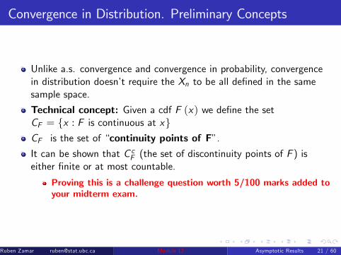
Unlike a.s. convergence and convergence in probability, convergencein distribution doesn’t require the Xn to be all defined in the samesample space.
Technical concept: Given a cdf F (x) we define the setCF = x : F is continuous at xCF is the set of “continuity points of F”.It can be shown that C cF (the set of discontinuity points of F ) iseither finite or at most countable.
Proving this is a challenge question worth 5/100 marks added toyour midterm exam.
Ruben Zamar [email protected] () Module 12 Asymptotic Results 21 / 60

Convergence in Distribution. Preliminary Concepts
Unlike a.s. convergence and convergence in probability, convergencein distribution doesn’t require the Xn to be all defined in the samesample space.
Technical concept: Given a cdf F (x) we define the setCF = x : F is continuous at x
CF is the set of “continuity points of F”.It can be shown that C cF (the set of discontinuity points of F ) iseither finite or at most countable.
Proving this is a challenge question worth 5/100 marks added toyour midterm exam.
Ruben Zamar [email protected] () Module 12 Asymptotic Results 21 / 60

Convergence in Distribution. Preliminary Concepts
Unlike a.s. convergence and convergence in probability, convergencein distribution doesn’t require the Xn to be all defined in the samesample space.
Technical concept: Given a cdf F (x) we define the setCF = x : F is continuous at xCF is the set of “continuity points of F”.
It can be shown that C cF (the set of discontinuity points of F ) iseither finite or at most countable.
Proving this is a challenge question worth 5/100 marks added toyour midterm exam.
Ruben Zamar [email protected] () Module 12 Asymptotic Results 21 / 60

Convergence in Distribution. Preliminary Concepts
Unlike a.s. convergence and convergence in probability, convergencein distribution doesn’t require the Xn to be all defined in the samesample space.
Technical concept: Given a cdf F (x) we define the setCF = x : F is continuous at xCF is the set of “continuity points of F”.It can be shown that C cF (the set of discontinuity points of F ) iseither finite or at most countable.
Proving this is a challenge question worth 5/100 marks added toyour midterm exam.
Ruben Zamar [email protected] () Module 12 Asymptotic Results 21 / 60

Convergence in Distribution
Let F (x) be the cdf of the “target” rv X , and let CF be its set ofcontinuity points
Definition: We say that Xn converges in distribution to X andwrite Xn →d X if Fn (x)→ F (x) for all x ∈ CF .Note: the convergence of Fn (x) to F (x) may fail for points outsideCF
Ruben Zamar [email protected] () Module 12 Asymptotic Results 22 / 60

Convergence in Distribution
Let F (x) be the cdf of the “target” rv X , and let CF be its set ofcontinuity points
Definition: We say that Xn converges in distribution to X andwrite Xn →d X if Fn (x)→ F (x) for all x ∈ CF .
Note: the convergence of Fn (x) to F (x) may fail for points outsideCF
Ruben Zamar [email protected] () Module 12 Asymptotic Results 22 / 60

Convergence in Distribution
Let F (x) be the cdf of the “target” rv X , and let CF be its set ofcontinuity points
Definition: We say that Xn converges in distribution to X andwrite Xn →d X if Fn (x)→ F (x) for all x ∈ CF .Note: the convergence of Fn (x) to F (x) may fail for points outsideCF
Ruben Zamar [email protected] () Module 12 Asymptotic Results 22 / 60

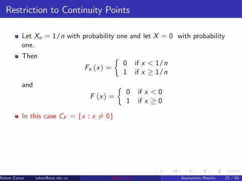
Restriction to Continuity Points
Let Xn = 1/n with probability one and let X = 0 with probabilityone.
Then
Fn (x) =0 if x < 1/n1 if x ≥ 1/n
and
F (x) =0 if x < 01 if x ≥ 0
In this case CF = x : x 6= 0Notice that Fn (0) = 0 for all n and F (0) = 1
That is, Fn (0)9 F (0) .
However, Fn (x)→ F (x) for all x 6= 0. Therefore 1/n→ 0 indistribution!
Ruben Zamar [email protected] () Module 12 Asymptotic Results 23 / 60
Restriction to Continuity Points
Let Xn = 1/n with probability one and let X = 0 with probabilityone.
Then
Fn (x) =0 if x < 1/n1 if x ≥ 1/n
and
F (x) =0 if x < 01 if x ≥ 0
In this case CF = x : x 6= 0
Notice that Fn (0) = 0 for all n and F (0) = 1
That is, Fn (0)9 F (0) .
However, Fn (x)→ F (x) for all x 6= 0. Therefore 1/n→ 0 indistribution!
Ruben Zamar [email protected] () Module 12 Asymptotic Results 23 / 60

Restriction to Continuity Points
Let Xn = 1/n with probability one and let X = 0 with probabilityone.
Then
Fn (x) =0 if x < 1/n1 if x ≥ 1/n
and
F (x) =0 if x < 01 if x ≥ 0
In this case CF = x : x 6= 0Notice that Fn (0) = 0 for all n and F (0) = 1
That is, Fn (0)9 F (0) .
However, Fn (x)→ F (x) for all x 6= 0. Therefore 1/n→ 0 indistribution!
Ruben Zamar [email protected] () Module 12 Asymptotic Results 23 / 60

Asymptotic Distribution of the Max of Unif(a,b)
Example: Suppose that X1,X2, ...,Xn are iid Unif (a, b)
We have shown above that
Vn = max X1,X2, ...,Xn →p b
We will show now that
n (b− Vn)→d Exp(
1b− a
)
Ruben Zamar [email protected] () Module 12 Asymptotic Results 24 / 60

Asymptotic Distribution of the Max of Unif(a,b)
Example: Suppose that X1,X2, ...,Xn are iid Unif (a, b)
We have shown above that
Vn = max X1,X2, ...,Xn →p b
We will show now that
n (b− Vn)→d Exp(
1b− a
)
Ruben Zamar [email protected] () Module 12 Asymptotic Results 24 / 60

Asymptotic Distribution of the Max of Unif(a,b)
Example: Suppose that X1,X2, ...,Xn are iid Unif (a, b)
We have shown above that
Vn = max X1,X2, ...,Xn →p b
We will show now that
n (b− Vn)→d Exp(
1b− a
)
Ruben Zamar [email protected] () Module 12 Asymptotic Results 24 / 60

Max of Unif(a,b) (continued)
We will first obtain the cdf for n (b− Vn) .
For any d > 0 such that d/n < b, we have
P [n (b− Vn) ≤ d ] = P[b− d
n≤ Vn
]= 1− P
[Vn < b−
dn
]= 1−
[(b− d
n
)− a
b− a
]n= 1−
[1− d
n (b− a)
]n
Ruben Zamar [email protected] () Module 12 Asymptotic Results 25 / 60

Max of Unif(a,b) (continued)
We will first obtain the cdf for n (b− Vn) .For any d > 0 such that d/n < b, we have
P [n (b− Vn) ≤ d ] = P[b− d
n≤ Vn
]= 1− P
[Vn < b−
dn
]= 1−
[(b− d
n
)− a
b− a
]n= 1−
[1− d
n (b− a)
]n
Ruben Zamar [email protected] () Module 12 Asymptotic Results 25 / 60

Max of Unif(a,b) (continued)
Recall that (1+
xn
)n→ ex , for all x as n→ ∞
Therefore
1−[1− d
n (b− a)
]n→ 1− exp
− db− a
, for all d > 0.
This is the cdf of an Exp( 1b−a)
Ruben Zamar [email protected] () Module 12 Asymptotic Results 26 / 60

Max of Unif(a,b) (continued)
Recall that (1+
xn
)n→ ex , for all x as n→ ∞
Therefore
1−[1− d
n (b− a)
]n→ 1− exp
− db− a
, for all d > 0.
This is the cdf of an Exp( 1b−a)
Ruben Zamar [email protected] () Module 12 Asymptotic Results 26 / 60

Max of Unif(a,b) (continued)
Recall that (1+
xn
)n→ ex , for all x as n→ ∞
Therefore
1−[1− d
n (b− a)
]n→ 1− exp
− db− a
, for all d > 0.
This is the cdf of an Exp( 1b−a)
Ruben Zamar [email protected] () Module 12 Asymptotic Results 26 / 60

Asymptotic Distribution of the Min of Unif(a,b)
The derivation of the asymptotic distribution of n (Un − a) is achallenge problem worth 1/100 increase in the midterm grade.
Ruben Zamar [email protected] () Module 12 Asymptotic Results 27 / 60

Convergence in Distribution and Continuity
It can be shown (this time with considerable level of diffi culty) thatconvergence in distribution is preserved by continuous functions
More precisely, if Xn →d X and g (x) is continuous, theng (Xn)→d g (X )
Example: Suppose that Xn →d X ∼ N (0, 1) Then
2+ 3Xn →d 2+ 3X ∼ N (2, 9)
Ruben Zamar [email protected] () Module 12 Asymptotic Results 28 / 60

Another Example
Example: Suppose that Xn →d X ∼ Unif (0, 1) . What is thelimiting distribution of − log (Xn)?
Solution: By continuity
− log (Xn)→d − log (X )
Moreover, for all y > 0,
P (− log (X ) ≤ y) = P (log (X ) ≥ −y)= P
(X ≥ e−y
)= 1− e−y
Therefore, − log (Xn)→d Exp (1)
Ruben Zamar [email protected] () Module 12 Asymptotic Results 29 / 60

Another Example
Example: Suppose that Xn →d X ∼ Unif (0, 1) . What is thelimiting distribution of − log (Xn)?Solution: By continuity
− log (Xn)→d − log (X )
Moreover, for all y > 0,
P (− log (X ) ≤ y) = P (log (X ) ≥ −y)= P
(X ≥ e−y
)= 1− e−y
Therefore, − log (Xn)→d Exp (1)
Ruben Zamar [email protected] () Module 12 Asymptotic Results 29 / 60

An important Technical Result (on MGF’s)
Suppose that Xn ∼ Fn and Mn (t) = E(etXn
), for all n
Suppose that X ∼ F and M (t) = E(etX)
Suppose that Mn (t)→ M (t) for all −ε < t < ε, for some ε > 0
Then Fn (x)→ F (x) for all x ∈ CFIn other words Mn (t)→ M (t) for all −ε < t < ε, for some ε > 0implies that Xn →d X .
Ruben Zamar [email protected] () Module 12 Asymptotic Results 30 / 60

An important Technical Result (on MGF’s)
Suppose that Xn ∼ Fn and Mn (t) = E(etXn
), for all n
Suppose that X ∼ F and M (t) = E(etX)
Suppose that Mn (t)→ M (t) for all −ε < t < ε, for some ε > 0
Then Fn (x)→ F (x) for all x ∈ CF
In other words Mn (t)→ M (t) for all −ε < t < ε, for some ε > 0implies that Xn →d X .
Ruben Zamar [email protected] () Module 12 Asymptotic Results 30 / 60

An important Technical Result (on MGF’s)
Suppose that Xn ∼ Fn and Mn (t) = E(etXn
), for all n
Suppose that X ∼ F and M (t) = E(etX)
Suppose that Mn (t)→ M (t) for all −ε < t < ε, for some ε > 0
Then Fn (x)→ F (x) for all x ∈ CFIn other words Mn (t)→ M (t) for all −ε < t < ε, for some ε > 0implies that Xn →d X .
Ruben Zamar [email protected] () Module 12 Asymptotic Results 30 / 60

The Central Limit Theorem (CLT)
Suppose that X1,X2, ...,Xn are iid with common mean µ andcommon variance σ2
Then
Zn =Xn − E (Xn)SD (Xn)
=√n(Xn − µ)
σ→d Z ∼ N (0, 1)
Ruben Zamar [email protected] () Module 12 Asymptotic Results 31 / 60

The Central Limit Theorem (CLT)
Suppose that X1,X2, ...,Xn are iid with common mean µ andcommon variance σ2
Then
Zn =Xn − E (Xn)SD (Xn)
=√n(Xn − µ)
σ→d Z ∼ N (0, 1)
Ruben Zamar [email protected] () Module 12 Asymptotic Results 31 / 60

CLT (continued)
To summarize, for large n (e.g. n ≥ 20)
√n(Xn − µ)
σ≈ N (0, 1)
⇒ Xn − µ ≈ σ√nN (0, 1) = N
(0,
σ2
n
)
⇒ Xn ≈ µ+N(0,
σ2
n
)= N
(µ,
σ2
n
)
⇒ Xn ≈ N [E (Xn) ,Var (Xn)]
Ruben Zamar [email protected] () Module 12 Asymptotic Results 32 / 60

CLT (continued)
To summarize, for large n (e.g. n ≥ 20)
√n(Xn − µ)
σ≈ N (0, 1)
⇒ Xn − µ ≈ σ√nN (0, 1) = N
(0,
σ2
n
)
⇒ Xn ≈ µ+N(0,
σ2
n
)= N
(µ,
σ2
n
)
⇒ Xn ≈ N [E (Xn) ,Var (Xn)]
Ruben Zamar [email protected] () Module 12 Asymptotic Results 32 / 60

CLT (continued)
To summarize, for large n (e.g. n ≥ 20)
√n(Xn − µ)
σ≈ N (0, 1)
⇒ Xn − µ ≈ σ√nN (0, 1) = N
(0,
σ2
n
)
⇒ Xn ≈ µ+N(0,
σ2
n
)= N
(µ,
σ2
n
)
⇒ Xn ≈ N [E (Xn) ,Var (Xn)]
Ruben Zamar [email protected] () Module 12 Asymptotic Results 32 / 60

CLT (continued)
To summarize, for large n (e.g. n ≥ 20)
√n(Xn − µ)
σ≈ N (0, 1)
⇒ Xn − µ ≈ σ√nN (0, 1) = N
(0,
σ2
n
)
⇒ Xn ≈ µ+N(0,
σ2
n
)= N
(µ,
σ2
n
)
⇒ Xn ≈ N [E (Xn) ,Var (Xn)]
Ruben Zamar [email protected] () Module 12 Asymptotic Results 32 / 60

CLT (continued)
Proof. We can assume without loss of generality that µ = 0 andσ2 = 1.
Challenge Question: Show that we can indeed assume that µ = 0and σ2 = 1 without loss of generality. This is for an increase of0.5/30 in your MT 2 grade.
Then Zn =√nXn and using the iid assumption:
MZn (t) = M√nXn (t)
= M(∑Xi )/√n (t)
= M∑Xi(t/√n)
=[M(t/√n)]n
Ruben Zamar [email protected] () Module 12 Asymptotic Results 33 / 60

CLT (continued)
Moreover,
M(t/√n)= E
exp
(tX1√n
)= E
1+
tX1√n+t2X 212n
+ o
(t√n
)
= 1+t2
2n+ o
(t√n
)
Ruben Zamar [email protected] () Module 12 Asymptotic Results 34 / 60

CLT (continued)
Hence
M(t/√n)n=
[1+
t2
2n+ o
(t√n
)]n→ exp
(t2
2
)which is the MGF of a standard normal random variable. This provesthe result.
Ruben Zamar [email protected] () Module 12 Asymptotic Results 35 / 60

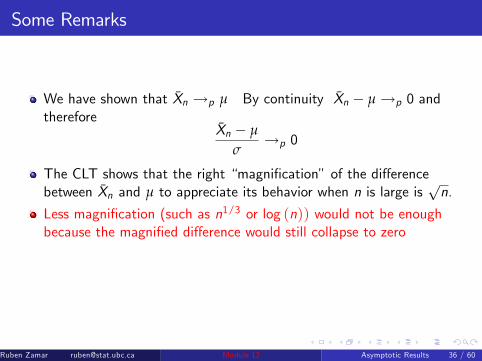
Some Remarks
We have shown that Xn →p µ By continuity Xn − µ→p 0 andtherefore
Xn − µ
σ→p 0
The CLT shows that the right “magnification”of the differencebetween Xn and µ to appreciate its behavior when n is large is
√n.
Less magnification (such as n1/3 or log (n)) would not be enoughbecause the magnified difference would still collapse to zero
More magnification (such as n3 or en ) would be to much because themagnified absolute difference would blow out to infinity.
Ruben Zamar [email protected] () Module 12 Asymptotic Results 36 / 60

Bounded in Probability
A normal random variable is unbounded (it can take any valuebetween −∞ and ∞)
However Z ∼ N (0, 1) is bounded in probability because theP (|Z | > K ) = 2 (1−Φ (K ))→ 0 as K → ∞.A sequence Yn is bounded in probability if for all δ > 0, there existsKδ > 0 and Nδ > 0 such that
P (|Yn | ≤ Kδ) ≥ 1− δ,
for all n ≥ Nδ.
Ruben Zamar [email protected] () Module 12 Asymptotic Results 37 / 60

Bounded in Probability
A normal random variable is unbounded (it can take any valuebetween −∞ and ∞)However Z ∼ N (0, 1) is bounded in probability because theP (|Z | > K ) = 2 (1−Φ (K ))→ 0 as K → ∞.
A sequence Yn is bounded in probability if for all δ > 0, there existsKδ > 0 and Nδ > 0 such that
P (|Yn | ≤ Kδ) ≥ 1− δ,
for all n ≥ Nδ.
Ruben Zamar [email protected] () Module 12 Asymptotic Results 37 / 60

Bounded in Probability
A normal random variable is unbounded (it can take any valuebetween −∞ and ∞)However Z ∼ N (0, 1) is bounded in probability because theP (|Z | > K ) = 2 (1−Φ (K ))→ 0 as K → ∞.A sequence Yn is bounded in probability if for all δ > 0, there existsKδ > 0 and Nδ > 0 such that
P (|Yn | ≤ Kδ) ≥ 1− δ,
for all n ≥ Nδ.
Ruben Zamar [email protected] () Module 12 Asymptotic Results 37 / 60

Bounded in Probability and the CLT
The CLT also means that the difference∣∣√n (Xn − µ)
∣∣ is boundedin probability
Notation: Xn − µ = Op(1/√n)meaning that∣∣∣∣ Xn − µ
1/√n
∣∣∣∣ = ∣∣√n (Xn − µ)∣∣ is bounded in probability
Ruben Zamar [email protected] () Module 12 Asymptotic Results 38 / 60

Bounded in Probability and the CLT
The CLT also means that the difference∣∣√n (Xn − µ)
∣∣ is boundedin probability
Notation: Xn − µ = Op(1/√n)meaning that∣∣∣∣ Xn − µ
1/√n
∣∣∣∣ = ∣∣√n (Xn − µ)∣∣ is bounded in probability
Ruben Zamar [email protected] () Module 12 Asymptotic Results 38 / 60

CLT ApplicationNormal Approximation for the Binomial
Suppose that Xn ∼ Binom (n, p)
Then
Xn = Y1 + Y2 + · · ·+ Yn, Yi ∼ iid Binom (1, p)
E (Yi ) = p, Var (Yi ) = p (1− p)
We can writeXnn=Y1 + Y2 + · · ·+ Yn
n= Yn
Ruben Zamar [email protected] () Module 12 Asymptotic Results 39 / 60

CLT ApplicationNormal Approximation for the Binomial
Suppose that Xn ∼ Binom (n, p)Then
Xn = Y1 + Y2 + · · ·+ Yn, Yi ∼ iid Binom (1, p)
E (Yi ) = p, Var (Yi ) = p (1− p)
We can writeXnn=Y1 + Y2 + · · ·+ Yn
n= Yn
Ruben Zamar [email protected] () Module 12 Asymptotic Results 39 / 60

CLT ApplicationNormal Approximation for the Binomial
Suppose that Xn ∼ Binom (n, p)Then
Xn = Y1 + Y2 + · · ·+ Yn, Yi ∼ iid Binom (1, p)
E (Yi ) = p, Var (Yi ) = p (1− p)
We can writeXnn=Y1 + Y2 + · · ·+ Yn
n= Yn
Ruben Zamar [email protected] () Module 12 Asymptotic Results 39 / 60

CLT Application (continued)Normal Approximation for the Binomial
By the CLT,
√n
(Xnn − p√p (1− p)
)=√n
(Yn − p√p (1− p)
)→ Z ∼ N (0, 1)
This means that
√n
(Xnn − p√p (1− p)
)w N (0, 1)
Ruben Zamar [email protected] () Module 12 Asymptotic Results 40 / 60

CLT Application (continued)Normal Approximation for the Binomial
By the CLT,
√n
(Xnn − p√p (1− p)
)=√n
(Yn − p√p (1− p)
)→ Z ∼ N (0, 1)
This means that
√n
(Xnn − p√p (1− p)
)w N (0, 1)
Ruben Zamar [email protected] () Module 12 Asymptotic Results 40 / 60

CLT Application (continued)Normal Approximation for the Binomial
Therefore
=⇒Xnn − p√p (1− p)
w 1√nN (0, 1) = N
(0,1n
)
=⇒ Xnn− p w
√p (1− p)N
(0,1n
)= N
(0,p (1− p)
n
)
=⇒ Xnnw p +N
(0,p (1− p)
n
)= N
(p,p (1− p)
n
)
=⇒ Xn w nN(p,p (1− p)
n
)= N
(np,
n2p (1− p)n
)
Ruben Zamar [email protected] () Module 12 Asymptotic Results 41 / 60

CLT Application (continued)Normal Approximation for the Binomial
In summary
Binomial (n, p) w N (np, np (1− p)) = N (E (Xn) ,Var (Xn))
That is, when n is large and p is not too small (so that the originaldistribution is not too asymmetric)
Rule of thumb: min np, n (1− p) ≥ 5
Ruben Zamar [email protected] () Module 12 Asymptotic Results 42 / 60

CLT Application (continued)Normal Approximation for the Binomial
As a numerical example, let X ∼ Binom (20, 0.4)
Use the normal distribution to approximate
(a) P (X ≥ 6) (b) P (6 < X < 9)
Solution
E (X ) = 20× 0.4 = 8,Var (X ) = 20× 0.4× 0.6 = 4.8SD (X ) =
√4.8 = 2.1909
Ruben Zamar [email protected] () Module 12 Asymptotic Results 43 / 60

CLT Application (continued)Normal Approximation for the Binomial
As a numerical example, let X ∼ Binom (20, 0.4)Use the normal distribution to approximate
(a) P (X ≥ 6) (b) P (6 < X < 9)
Solution
E (X ) = 20× 0.4 = 8,Var (X ) = 20× 0.4× 0.6 = 4.8SD (X ) =
√4.8 = 2.1909
Ruben Zamar [email protected] () Module 12 Asymptotic Results 43 / 60

CLT Application (continued)
(a)
P (X ≥ 6) = 1− P (X < 6) = 1− P (X ≤ 5)
= 1−Φ(5− 82.1909
)= 1−Φ (−1.3693)
= 0.9145472
Ruben Zamar [email protected] () Module 12 Asymptotic Results 44 / 60

CLT Application (continued)
(b)
P (6 < X < 9) = P (6 < X ≤ 8)
= Φ(8− 82.1909
)−Φ
(6− 82.1909
)= 0.5−Φ (−0.91287) = 0.3193445
Ruben Zamar [email protected] () Module 12 Asymptotic Results 45 / 60

CLT Application (continued)Normal Approximation for the Binomial
The exact probability calculated using the Binomial distribution are0.874401 and 0.3455881
With “correction for discreteness”we have
1−Φ(5.5−82.1909
)= 1−Φ (−1.1411) = 0.8730858 and
Φ(8.5−82.1909
)−Φ
(6.5−82.1909
)= Φ (0.228 22)−Φ (−0.68465) = 0.34348
Fortunately for all of us, these approximations are nowadaysobsolete as the exact quantities can be easily computed usingstatistical software.
Ruben Zamar [email protected] () Module 12 Asymptotic Results 46 / 60

CLT ApplicationMonte Carlo Integration
Suppose we wish to compute the integral
A =∫ b
ag (x) dx
We notice that
I = (b− a) 1b− a
∫ b
ag (x) dx
= (b− a)E g (U) , U ∼ Unif (a, b)
= (b− a)A, A = E g (U)Therefore
I = (b− a)A, where A = E g (U) .
Ruben Zamar [email protected] () Module 12 Asymptotic Results 47 / 60

CLT ApplicationMonte Carlo Integration
Suppose we wish to compute the integral
A =∫ b
ag (x) dx
We notice that
I = (b− a) 1b− a
∫ b
ag (x) dx
= (b− a)E g (U) , U ∼ Unif (a, b)
= (b− a)A, A = E g (U)
ThereforeI = (b− a)A, where A = E g (U) .
Ruben Zamar [email protected] () Module 12 Asymptotic Results 47 / 60

CLT ApplicationMonte Carlo Integration
Suppose we wish to compute the integral
A =∫ b
ag (x) dx
We notice that
I = (b− a) 1b− a
∫ b
ag (x) dx
= (b− a)E g (U) , U ∼ Unif (a, b)
= (b− a)A, A = E g (U)Therefore
I = (b− a)A, where A = E g (U) .
Ruben Zamar [email protected] () Module 12 Asymptotic Results 47 / 60

CLT Application (Continued)Monte Carlo Integration
Monte Carlo Integration Method:
1 generate a large enough number N of iid Ui with common distributionUnif (a, b)
2 Estimate the “population mean” A by the “sample mean” A, where
A =1N
N
∑i=1
g (Ui )
Ruben Zamar [email protected] () Module 12 Asymptotic Results 48 / 60

CLT Application (Continued)Monte Carlo Integration
Monte Carlo Integration Method:1 generate a large enough number N of iid Ui with common distributionUnif (a, b)
2 Estimate the “population mean” A by the “sample mean” A, where
A =1N
N
∑i=1
g (Ui )
Ruben Zamar [email protected] () Module 12 Asymptotic Results 48 / 60

CLT Application (Continued)
Properties of the Monte Carlo Estimate
1 A is an unbiased estimate of A : E(A)= A
Because the sample mean is an unbiased estimate of the populationmean
2 A→ A a.s. (and also in probability)Because of the SLLN (and the WLLN)
3√N(A− A
)→d N
(0, τ2
), where τ2 = Var (g (U)) (by the CLT)
4 τ2 = (1/N)∑ g2 (Ui )− [(1/N)∑ g (Ui )]→ τ2 a.s. (and also inprobability)Because of the SLLN (and the WLLN)
Ruben Zamar [email protected] () Module 12 Asymptotic Results 49 / 60

CLT Application (Continued)
Properties of the Monte Carlo Estimate1 A is an unbiased estimate of A : E
(A)= A
Because the sample mean is an unbiased estimate of the populationmean
2 A→ A a.s. (and also in probability)Because of the SLLN (and the WLLN)
3√N(A− A
)→d N
(0, τ2
), where τ2 = Var (g (U)) (by the CLT)
4 τ2 = (1/N)∑ g2 (Ui )− [(1/N)∑ g (Ui )]→ τ2 a.s. (and also inprobability)Because of the SLLN (and the WLLN)
Ruben Zamar [email protected] () Module 12 Asymptotic Results 49 / 60
Slutzky’s Results
Suppose that Xn →d X and Yn →p c. Then
(a) Xn + Yn →d X + c(b) XnYn →d Xc(c) XnYn →d X/c , provided c 6= 0.
Ruben Zamar [email protected] () Module 12 Asymptotic Results 50 / 60

Slutzky’s Results
Suppose that Xn →d X and Yn →p c. Then
(a) Xn + Yn →d X + c
(b) XnYn →d Xc(c) XnYn →d X/c , provided c 6= 0.
Ruben Zamar [email protected] () Module 12 Asymptotic Results 50 / 60

Slutzky’s Results
Suppose that Xn →d X and Yn →p c. Then
(a) Xn + Yn →d X + c(b) XnYn →d Xc
(c) XnYn →d X/c , provided c 6= 0.
Ruben Zamar [email protected] () Module 12 Asymptotic Results 50 / 60

Slutzky’s Results
Suppose that Xn →d X and Yn →p c. Then
(a) Xn + Yn →d X + c(b) XnYn →d Xc(c) XnYn →d X/c , provided c 6= 0.
Ruben Zamar [email protected] () Module 12 Asymptotic Results 50 / 60

Application of Slutzky’s Results to MC Integration
By property 3 we have
√N
(A− A
)τ
→d N (0, 1) (*)
By property 4 we haveτ2 →p τ2
By continuity we also have
τ →p τ
andτ
τ→p 1 (**)
Ruben Zamar [email protected] () Module 12 Asymptotic Results 51 / 60

Application of Slutzky’s Results to MC Integration
By property 3 we have
√N
(A− A
)τ
→d N (0, 1) (*)
By property 4 we haveτ2 →p τ2
By continuity we also have
τ →p τ
andτ
τ→p 1 (**)
Ruben Zamar [email protected] () Module 12 Asymptotic Results 51 / 60

Application of Slutzky’s Results to MC Integration
By property 3 we have
√N
(A− A
)τ
→d N (0, 1) (*)
By property 4 we haveτ2 →p τ2
By continuity we also have
τ →p τ
andτ
τ→p 1 (**)
Ruben Zamar [email protected] () Module 12 Asymptotic Results 51 / 60

Application of Slutzky’s Results to MC Integration(continued)
By (*), (**), and Slutzky’s Result (c) we have
√N
(A− A
)τ
τ
τ→d N (0, 1)
That is√N
(A− A
)τ
→d N (0, 1)
In summary,
A w N(A,
τ2
N
)
Ruben Zamar [email protected] () Module 12 Asymptotic Results 52 / 60

Application of Slutzky’s Results to MC Integration(continued)
By (*), (**), and Slutzky’s Result (c) we have
√N
(A− A
)τ
τ
τ→d N (0, 1)
That is√N
(A− A
)τ
→d N (0, 1)
In summary,
A w N(A,
τ2
N
)
Ruben Zamar [email protected] () Module 12 Asymptotic Results 52 / 60

Application of Slutzky’s Results to MC Integration(continued)
By (*), (**), and Slutzky’s Result (c) we have
√N
(A− A
)τ
τ
τ→d N (0, 1)
That is√N
(A− A
)τ
→d N (0, 1)
In summary,
A w N(A,
τ2
N
)
Ruben Zamar [email protected] () Module 12 Asymptotic Results 52 / 60

Controlling the MC-Integration Error
Fix the desired estimation precision (or relative precision): ε
Fix the desired probability of achieving the desired estimationprecision: 1− α
Run an “appropriate sized”pilot sample to calculate τ0
Ruben Zamar [email protected] () Module 12 Asymptotic Results 53 / 60

Controlling the MC-Integration Error
Notice that
P(∣∣A− A∣∣ < ε
)= P
(√N
∣∣∣∣ A− Aτ
∣∣∣∣ < √N ε
τ
)≈ 2Φ
(√N
ε
τ
)− 1
≈ 2Φ(√
Nε
τ0
)− 1
Ruben Zamar [email protected] () Module 12 Asymptotic Results 54 / 60

Controlling the MC-Integration Error
Solve for N in the following equation:
2Φ(√
Nε
τ0
)− 1 = 1− α
N∗ =
[τ0ε
Φ−1(1− α
2
)]2
Ruben Zamar [email protected] () Module 12 Asymptotic Results 55 / 60

Numerical Example
Example: Calculate the integral
I =1√2π
∫ 1.5
−0.5exp
(−12x2)dx
within a 0.001 error margin with probability 0.999.
In this case ε = 0.001 and α = 0.0001, b− a = 2,
g (x) = exp(−12x2)
and
A =12
∫ 1.5
−0.5exp
(−12x2)dx
Ruben Zamar [email protected] () Module 12 Asymptotic Results 56 / 60

Numerical Example (Continued)
Hence
I =2√2πA =
√2πA
We generate (using R) 100000 iid Unif (−0.5, 1.5) random variablesUi to compute
τ20 =11000
N
∑i=1
[exp
(−12U2i
)]2−[11000
N
∑i=1exp
(−12U2i
)]2
=11000
N
∑i=1exp
(−U2i
)−[11000
N
∑i=1exp
(−12U2i
)]2= 0.0457856
τ0 = 0.2139757
Ruben Zamar [email protected] () Module 12 Asymptotic Results 57 / 60

Numerical Example (Continued)
Therefore
N∗ =
[τ0ε
Φ−1(1− α
2
)]2
=
[0.21397570.001
Φ−1(1− 0.0001
2
)]2N∗ = 693, 044 (rounding up)
Ruben Zamar [email protected] () Module 12 Asymptotic Results 58 / 60

Numerical Example (Continued)
Now we generate 693, 044 iid Unif (−0.5, 1.5) random variables Ui tocompute
A =1N∗
N ∗
∑i=1exp
(−12U2i
)= 0.782887
Therefore
I =
√2πA =
√2π0.7830537 = 0.624654
Compare with
pnorm(1.5)− pnorm(−0.5) = 0.6246553
∣∣I − [pnorm(1.5)− pnorm(−0.5)]∣∣ = 0.000002
Ruben Zamar [email protected] () Module 12 Asymptotic Results 59 / 60

Numerical Example (Continued)
Now we generate 693, 044 iid Unif (−0.5, 1.5) random variables Ui tocompute
A =1N∗
N ∗
∑i=1exp
(−12U2i
)= 0.782887
Therefore
I =
√2πA =
√2π0.7830537 = 0.624654
Compare with
pnorm(1.5)− pnorm(−0.5) = 0.6246553
∣∣I − [pnorm(1.5)− pnorm(−0.5)]∣∣ = 0.000002Ruben Zamar [email protected] () Module 12 Asymptotic Results 59 / 60

Numerical Example (Continued)
In practice we don’t know I
Still we may wish to check if the desired precision has been likelyachieved
Recompute N∗∗ using the full Monte Carlo sample
N∗∗ = 692, 553
Compare N∗∗ with N∗
N∗∗ = 692, 553 < N∗ = 693, 044
Ruben Zamar [email protected] () Module 12 Asymptotic Results 60 / 60