stat 135 lab 10 two-way anova, randomized block design and ... · two-way anova suppose that a...
TRANSCRIPT
STAT 135 Lab 10Two-Way ANOVA, Randomized Block Design
and Friedman’s Test
Rebecca Barter
April 13, 2015

Two-way ANOVA
Two-way ANOVA
Let’s now imagine a dataset for which our response variable, Y ,may be influenced by two factors, each of which are potentialsources of variation.
I The first factor has I levels
I The second factor has J levels
Each combination (i, j) defines a treatment pairing. There area total of IJ treatment pairs.
We assume that we have K > 1 replicates for each treatmentcombination (i, j).
Two-way ANOVA
The idea is that we want to simultaneously examine the effectsof the two treatments/factors, and their interaction, on theresponse.
So we actually conduct 3 F -tests (one for each factor and onefor their interaction)
I To test if factor A has an effect:I compare the variability between the groups of factor A to
the “within” variability
I To test if factor B has an effect:I compare the variability between the groups of factor B to
the “within” variability
I To test if there is an interaction effect between A and B:I compare the variability between each combination of the
groups of factor A and of factor B to the “within”variability
Two-way ANOVA
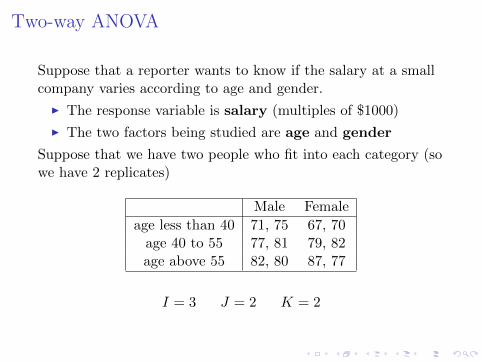
Suppose that a reporter wants to know if the salary at a smallcompany varies according to age and gender.
I The response variable is salary (multiples of $1000)
I The two factors being studied are age and gender
Suppose that we have two people who fit into each category (sowe have 2 replicates)
Male Female
age less than 40 71, 75 67, 70age 40 to 55 77, 81 79, 82age above 55 82, 80 87, 77
I = 3 J = 2 K = 2

Two-way ANOVA
Let’s introduce some notation:
I Yijk is the kth observation in the ith row and jth column.
I Y i·· is the mean of all observations in the ith row
I Y ·j· is the mean of all observations in the jth column
I Y ij· is the mean of all observations in the (i, j)th cell
I Y ··· is the mean of all observations
where a · in the subscript indicates what we are averaging over.
Two-way ANOVA
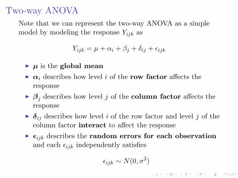
Note that we can represent the two-way ANOVA as a simplemodel by modeling the response Yijk as
Yijk = µ+ αi + βj + δij + εijk
I µ is the global mean
I αi describes how level i of the row factor affects theresponse
I βj describes how level j of the column factor affects theresponse
I δij describes how level i of the row factor and level j of thecolumn factor interact to affect the response
I εijk describes the random errors for each observationand each εijk independently satisfies
εijk ∼ N(0, σ2)
Two-way ANOVA
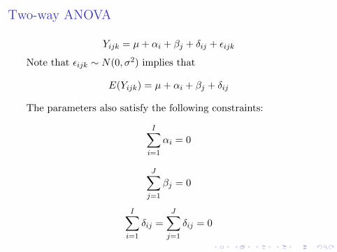
Yijk = µ+ αi + βj + δij + εijk
Note that εijk ∼ N(0, σ2) implies that
E(Yijk) = µ+ αi + βj + δij
The parameters also satisfy the following constraints:
I∑i=1
αi = 0
J∑j=1
βj = 0
I∑i=1
δij =
J∑j=1
δij = 0

Two-way ANOVA
Yijk = µ+ αi + βj + δij + εijk
We can calculate maximum likelihood estimates of each of theseparameters:
µ̂ = Y ··· global mean
α̂i = Y i·· − Y ··· differential effects for the row factor
β̂j = Y ·j· − Y ··· differential effects for the column factor
δ̂ij = Y ij· − µ̂− α̂i − β̂j interaction effect

Two-way ANOVA
For our example:
Male Female
age less than 40 71, 75 67, 70age 40 to 55 77, 81 79, 82age above 55 82, 80 87, 77
The mean over each age group is given by:
Y 1·· =71 + 75 + 67 + 70
2× 2= 70.75
Y 2·· =77 + 81 + 79 + 82
2× 2= 79.75
Y 3·· =82 + 80 + 87 + 77
2× 2= 81.50

Two-way ANOVA
For our example:
Male Female
age less than 40 71, 75 67, 70age 40 to 55 77, 81 79, 82age above 55 82, 80 87, 77
The mean over each gender is given by:
Y ·1· =71 + 75 + 77 + 81 + 82 + 80
3× 2= 77.67
Y ·2· =67 + 70 + 79 + 82 + 87 + 77
3× 2= 77.00

Two-way ANOVA
For our example:
Male Female
age less than 40 71, 75 67, 70age 40 to 55 77, 81 79, 82age above 55 82, 80 87, 77
The mean over each gender/age combination is given by:
Y 11· =71 + 75
2= 73.0 Y 12· =
67 + 70
2= 68.5
Y 21· =77 + 81
2= 79.0 Y 22· =
79 + 82
2= 80.5
Y 31· =82 + 80
2= 81.0 Y 32· =
87 + 77
283.0

Two-way ANOVA
For our example:
Male Female
age less than 40 71, 75 67, 70age 40 to 55 77, 81 79, 82age above 55 82, 80 87, 77
The global mean is given by:
Y ··· =71 + 75 + 67 + 77 + 81 + 79 + 82 + 82 + 80 + 87 + 77
3× 2× 2= 77.33

Two-way ANOVA
Like one-way ANOVA, the two-way ANOVA is conducted bycomparing various sum of squares. Recall that for one-wayANOVA we had
SST = SSB + SSW
where SSB was the between groups sum of squares and SSWwas the within groups sum of squares.

Two-way ANOVA
For two-way ANOVA, the total variability can be describedby the total sum of squares
SST =
I∑i=1
J∑j=1
K∑k=1
(Yijk − Y ···)2
and we will see that the total variability can be split up into thewithin-cell variability and the between-group variability, where
I The within-cell variability (often referred to as errors orresiduals) is defined by SSE (analog of SSW )
SSE =
I∑i=1
J∑j=1
K∑k=1
(Yijk − Y ij·)2

Two-way ANOVAI The between-cell variability can be split up into three
components (analog of SSB)I SSA: the sum of squares for the row factor
SSA =
I∑i=1
J∑j=1
K∑k=1
(Y i·· − Y ···)2 = JK
I∑i=1
(Y i·· − Y ···)2
I SSB : the sum of squares for the column factor
SSB =
I∑i=1
J∑j=1
K∑k=1
(Y ·j· − Y ···)2 = IK
J∑j=1
(Y ·j· − Y ···)2
I SSAB : the sum of squares for the interaction between therow and column factor
SSAB =
I∑i=1
J∑j=1
K∑k=1
(Y ij· − Y i·· − Y ·j· + Y ···)2
= K
I∑i=1
J∑j=1
(Y ij· − Y i·· − Y ·j· + Y ···)2
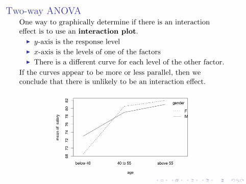
Two-way ANOVAOne way to graphically determine if there is an interactioneffect is to use an interaction plot.
I y-axis is the response level
I x-axis is the levels of one of the factors
I There is a different curve for each level of the other factor.
If the curves appear to be more or less parallel, then weconclude that there is unlikely to be an interaction effect.

Two-way ANOVA
There appears to be no interaction for the older age groupswith gender, but a bit of an interaction within the younger agegroups with gender. We will see that this is not enough toconclude that there is a significant interaction over all levels.

Two-way ANOVA
The sum of squares satisfy
SST = SSA + SSB + SSAB + SSE
and if we assume that εijk ∼ N(0, σ2), then
I SSE/σ2 ∼ χ2
IJ(K−1)
I SSA/σ2 ∼ χ2
I−1
I SSB/σ2 ∼ χ2
J−1
I SSAB/σ2 ∼ χ2
(I−1)(J−1)

Two-way ANOVA
The two-way ANOVA table is thus given by
Source df SS MS F
A (between) I − 1 SSA MSA MSA/MSEB (between) J − 1 SSB MSB MSB/MSE
AB (between) (I − 1)(J − 1) SSAB MSAB MSAB/MSEError (within) IJ(K − 1) SSE MSE
Total IJK − 1 SST
where
MS =SS
df

Two-way ANOVA
The p-value for testing the null hypothesis that there is nodifference between the levels of factor A is given by
P (FI−1,IJ(K−1) ≥MSA/MSE)
The p-value for testing the null hypothesis that there is nodifference between the levels of factor B is given by
P (FJ−1,IJ(K−1) ≥MSB/MSE)
The p-value for testing the null hypothesis that there is nointeraction between A and B is given by
P (F(I−1)(J−1),IJ(K−1) ≥MSAB/MSE)
Two-way ANOVA
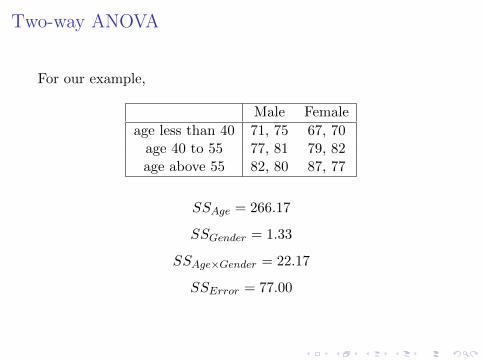
For our example,
Male Female
age less than 40 71, 75 67, 70age 40 to 55 77, 81 79, 82age above 55 82, 80 87, 77
SSAge = 266.17
SSGender = 1.33
SSAge×Gender = 22.17
SSError = 77.00

Two-way ANOVAFor our example:
Source df SS MS F
Gender 1 1.13 1.13 0.10Age 2 226.17 133.08 10.37
Age × Gender 2 22.17 11.08 0.86Error 6 77.00 12.83Total 11 366.67
and our p-values are:
Gender effect: P (F1,6 ≥ 0.10) = 0.76Age effect: P (F2,6 ≥ 10.37) = 0.011
Interaction effect: P (F2,6 ≥ 0.86) = 0.47
So we conclude that there is a difference in salary between thedifferent age groups but not for the different genders. Therealso does not appear to be a significant interaction effect.
Exercise

Exercise: Two-way ANOVA
Do the salary example in R, and report your results in a .pdfformat. Options include (but are not limited to):
I Using knitr (.Rnw file) – my preferred method (allows foreasy incorporation of LATEX, R code and figures)
I Using R Markdown (.Rmd file)
I Using IPython notebook
Randomized Block Design

Randomized Block DesignSuppose we have I treatments (e.g. fertilizers, diets) that wewant to try on each of I subjects (e.g. plots of land, people).
The I blocks for a subject might be
I physical partitions of the plot of land where a differentfertilizer is applied to each of the blocks
I stretches of time in each of which the same subject is puton a different diet.

Randomized Block Design
How is this different from one-way ANOVA?
I One-way ANOVA: we have a different group of J subjectsfor each of the I treatments
I Randomized Block Design: we have the same group of Jsubjects for each of the I treatments
How is this different from two-way ANOVA?
I Two-way ANOVA: Subjects are considered replicateswithin factors
I Randomized Block Design: Subjects are themselves a factor

Randomized Block Design
The observation in the (i, j)th block, Yij , is modeled by
Yij = µ+ αi + βj + εij
I µ is the overall mean parameterI αi is the differential effect of the ith treatment.
I Assume∑I
i=1 αi = 0.I βi is the differential effect of the jth subject.
I Assume∑J
j=1 βj = 0.I εij is the random error for the ith treatment on the jth
subject.
I Assume εijIID∼ N(0, σ2).

Randomized Block DesignThe total amount of variation is given by:
SST =
I∑i=1
J∑j=1
(Yij − Y )2
The variation explained by the treatment differential effect isgiven by:
SSA = J
I∑i=1
(Y i· − Y )2
The variation explained by the subject differential effect isgiven by:
SSB = I
J∑j=1
(Y ·j − Y )2
The variation not explained by the model is given by:
SSAB =
I∑i=1
J∑j=1
(Yij − Y i· − Y ·j + Y )2
Randomized Block Design
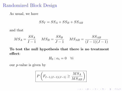
As usual, we have
SST = SSA + SSB + SSAB
and that
MSA =SSAI − 1
MSB =SSBJ − 1
MSAB =SSAB
(I − 1)(J − 1)
To test the null hypothesis that there is no treatmenteffect:
H0 : αi = 0 ∀i
our p-value is given by
P
(FI−1,(I−1)(J−1) ≥
MSAMSAB
)

Exercise

Exercise: Randomized block design (Rice 12.3 ExampleA)
Let’s consider an experimental study of drugs to relieve itching.
I 5 drugs were compared to a placebo and no drug (7treatments).
I 10 volunteers male subjects aged 20-30.
I Each volunteer underwent one treatment per day, and thetime-order was randomized.
I Individuals (rather than treatments) are the “blocks”.
I The subjects were given a drug (or placebo) intravenously,and itching was induced on their forearms.
I The subjects recorded the duration of the itching.

Exercise: Randomized block design (Rice 12.3 ExampleA)
The following table recorded the durations of the itching (inseconds) for the first 5 subjects.
Subject No Drug Placebo Papa. Morph. Amino. Pento. Tripelen.
BG 174 263 105 199 141 108 141JF 224 213 103 143 168 341 184BS 260 231 145 113 78 159 125SI 225 291 103 225 164 135 227
BW 165 168 144 176 127 239 194
Test the null hypothesis that there is no difference in meansbetween the different treatments.

Friedman’s Test (non-parametric version ofthe Randomized block design)

Friedman’s Test
1. Calculate the ranks of each treatment within each of theJ blocks (rather than overall). Rij is the rank of the ithtreatment for the jth subject for the jth subject.
2. Compute
Q =12
I(I + 1)SSA =
12J
I(I + 1)
I∑i=1
(Ri· −R
)2 ∼ χ2I−1
To test the null hypothesis that there is no treatment effect, thep-value is given by
P (χ2I−1 ≥ Q)

Exercise

Exercise: Friedman’s test (Rice 12.4 Example A)
Do the previous example using a non-parametric method.