stanislaus – lower san-joaquin river water temperature ... · pdf fileand the main-stem...
TRANSCRIPT

Stanislaus – Lower San-Joaquin River Water Temperature Modeling and Analysis
Lower Stanislaus River Goodwin Tulloch New Melones
Prepared for: CALFED
ERP-02-P28
Prepared by: AD Consultants
Resource Management Associates, Inc. Watercourse Engineering, Inc.
April 2007
DWR-1086

Stanislaus-Lower SJR Water Temperature Model
StanTempModelFinal-Apr-2007.doc i
STANISLAUS RIVER WATER TEMPERATURE MODEL
EXECUTIVE SUMMARY
In the late 1990s a group of stakeholders on the Stanislaus River initiated a cooperative effort to develop a water temperature model for the Stanislaus River having recognized the need to analyze the relationship between operational alternatives, water temperature regimes and fish mortality in the Stanislaus River. These stakeholders included the U.S. Bureau of Reclamation (USBR), Fish and Wildlife Service (USFWS), California Department of Fish & Game (CDFG), Oakdale Irrigation District (OID), South San Joaquin Irrigation District (SSJID), and Stockton East Water District (SEWD).
In December 1999, these partners garnered the necessary funding and, through a cost sharing arrangement, retained AD Consultants in association with its sub-consultant Research Management Associates to develop the model and perform a preliminary analysis of operational alternatives. In addition, the cost-sharing partners launched an extensive program for water temperature and meteorological data collection throughout the Stanislaus River Basin, in support of the modeling effort.
In 2002, the stakeholders decided unanimously to accept the model and adopt it as the primary water temperature planning tool for the Stanislaus River. Nevertheless, the stakeholders recognized the need to extend the model to the Lower San Joaquin River, thus enabling to study the relationship between Stanislaus operation and the temperature regime in the lower San Joaquin River enroute to the Bay-Delta.
In 2003 the project was extended to include the lower San Joaquin River through a CALFED grant (ERP-02-P28) to Tri-Dam (recipient) which is the subject of this report.
In December 2004, CALFED decided to extend the Stanislaus – Lower San Joaquin River Water Temperature Model to include the Tuolumne and Merced rivers, and the main-stem San Joaquin River from Stevenson to Mossdale (to be known as the San Joaquin River (SJR) Basin-Wide Water Temperature Model). The work was to be performed in two stages: 1) Through an amendment to the existing recipient agreement with Tri-Dam (ERP-02-P28), and 2) through a two-year Directed Action, thereafter.
Under the amended scope, the recipient was to develop a beta version of the model by the end of the current agreement period (October, 2006). This work has already been accomplished, presented to CALFED and approved through a CALFED sponsored peer review. The Directed Action was to allow further refinement of the model and use the model to investigate various mechanisms for water temperature improvements, both through operational and/or structural measures at existing facilities in all three tributaries of the San Joaquin River. This work commenced in October 2006.
The Model
The Stanislaus Water Temperature Model is based on the HEC-5Q computer simulation model designed to simulate the thermal regime of mainstem reservoirs and
Stanislaus-Lower SJR Water Temperature Model
StanTempModelFinal-Apr-2007.doc ii
river reaches. The extent of the model includes New Melones Reservoir, Tulloch Reservoir, Goodwin Pool, and approximately 60 miles of the Stanislaus River from Goodwin Dam to the confluence with the San Joaquin River (SJR) and the San Joaquin River from the Tuolumne River to Mossdale.
The objectives of this effort were to develop and calibrate a model capable of simulating the water temperature responses in the Stanislaus River system and to evaluate the impacts of New Melones Reservoir operations on downstream water temperatures. The model is designed to provide a basin-wide evaluation of temperature impacts at 6-hour intervals for alternative conditions such as changes in system operation.
The HEC-5Q model of the Stanislaus River system was previously calibrated to 1990 –1999 data. The current effort involves refinement of the initial calibration based on additional, detailed data available for the five year period from 2000 through 2004, including reservoir temperature profile observations in New Melones Reservoir, Tulloch Reservoir, and Goodwin Reservoir, as well as temperature time series observations at several stations in the Stanislaus River and Lower San Joaquin River. Minor adjustments have been made to model coefficients during the current calibration; however, previous calibration results remain relevant representations of model performance. Simulated flow conditions were developed using the CALSIM II model as well as those developed by Stakeholders. This model allows simulating the operations of New Melones and Tulloch reservoirs, given projected water demands and operational agreements in the basin.
Temperature Objectives The Stanislaus Water Temperature Model is driven by water temperature
objectives at critical points in the river system that would enhance habitat conditions for anadromous fish (e.g., fall-run Chinook salmon). A peer review panel (Panel) was assembled to evaluate the biological merits, and application of thermal criteria in assessment of model generated alternatives for the Stanislaus River. The Panel consisted of John Bartholow, United States Geological Survey; Chuck Hanson, Hanson Environmental; and Chris Myrick, Colorado State University. This group included scientists with local expertise, relevant discipline knowledge, as well as experience outside the Delta or Bay-Delta water issues.
A critical Panel conclusion was that a two threshold (e.g., optimal, suboptimal, and lethal ranges) criteria did not necessarily differentiate simulated alternatives on a broad scale. Further, from the outset of this review, the Panel had concerns over the discontinuous format of the two threshold (three-range) criteria - specifically, the inability of the discrete ranges to represent the continuous physiological response of a particular life stage. As an alternative, the Panel developed a thermal criteria for various life stages (e.g., adult migration, egg incubation, juvenile rearing) of anadromous fish based on 7-day average of the maximum daily temperatures (7DADM), wherein thermal status (e.g., stress) is represented by a continual, but exponentially increasing function with increasing temperature. In addition to the weekly average criteria, single day maximum temperatures were also considered because short duration elevated temperature events (on the order of a few hours) can have profound impacts on
Stanislaus-Lower SJR Water Temperature Model
StanTempModelFinal-Apr-2007.doc iii
anadromous fish populations. Thus, an additional metric representing a one-day instantaneous maximum lethal water temperature was developed based on an upper incipient lethal condition. The Panel encouraged the modification of such criteria, as necessary, by local resource managers when assessing model-simulated alternatives if there was supporting evidence to refine the criteria for the Stanislaus River.
Model Application Subsequent to model calibration and development of thermal criteria was the
application of the model to a wide range of alternatives for water temperature management in the Stanislaus River and lower San Joaquin River. These alternatives consisted of operational changes, physical changes of existing facilities, and combinations of the two. The alternatives studied with the model were divided into two general categories:
1) Water Management Plans – operational options consisting of diversions and instream flow schedules proposed by stakeholders, primarily the water irrigation districts and the fishery agencies.
2) Other Operational and Physical Changes – other concepts that were developed through discussions with the stakeholders or initiated by the project team. These concepts are stand-alone options and, if feasible, could be implemented in conjunction with the Water Management Plans.
Water Management Plans The water management plan proposed by the Districts included simulated
deliveries to OID and SSJID and subscribed deliveries to SEWD and CSJWCD, fish flow, and water quality releases based on CALSIM II simulations. The temperature criteria were modified in terms of magnitude and location of control points for the various life stages. CDFG proposed two water management plans: fish and water quality schedule with spring flow variations only (CFDG1); and fish and water quality schedule with spring, summer, and fall flow variations (CDFG2). Release schedules were year-type dependent and thermal criteria were applied at control point locations that were also year-type dependent.
From the temperature response point of view, the results differ among the alternatives, but generally late spring and early fall present the most challenging periods for anadromous fish in the river. In the spring period, the Districts’ case and criteria provides the best performance. During the summer period, the CDFG1 Case, with either the Peer or CDFG Criteria, provides the best performance. In the fall, both the CDFG1 and CDFG2 Cases provide improvement over historic conditions. The District Case shows reduced penalty, but this reduction varies considerably among the selected criteria, at times accruing more penalty than the historic condition. Other Operational and Physical Changes
Other operational and physical changes consisted of a wide range of operations and capital projects that may expand temperature management control in the Stanislaus River. These changes included:
Stanislaus-Lower SJR Water Temperature Model
StanTempModelFinal-Apr-2007.doc iv
• Tulloch re-operation (September drawdown and filling)
• New Melones power bypass with and without Old Melones Dam (various dates)
• Goodwin Dam Retrofit (lower level outlet)
• New Melones selective withdrawal (with and without Old Melones Dam)
• New Melones power intake extension (without old dam)
• Old Melones Dam removal
• Old Melones lowered 55 feet (partial removal) Briefly, re-operation of Tulloch has little merit with or without New Melones
power plant bypass. Conversely, power bypass provides cooler temperatures during the fall months without any structural changes; however, bypass decisions should consider temperature benefits versus foregone power costs.
The Goodwin retrofit option provides a modest reduction of the maximum temperature below Goodwin Dam throughout the spring, summer and fall months of all years
New Melones selective withdrawal provides greater flexibility for controlling outflow temperatures without foregoing power production. Temperature reductions are of the same magnitude as power bypass, so a selective withdrawal implementation plan should be based on temperature benefits versus construction and O&M costs. Extension of the power intake to 675 feet alone depletes the cold water pool prematurely and compromises the potential for power bypass to control fall temperatures. Such an extension should only be considered as part of a selective withdrawal scheme.
Old Melones Dam removal or lowering alone has very little impact on release temperatures when water levels are above approximately 790 feet; however, it does make more water available when bypassing the power plant or if a selective withdrawal option is adopted. Considering the effort of total removal of Old Melones Dam versus partial removal, the notched dam (mid-dam notch approximately 100 feet wide to elevation 668 feet at 55 feet below the old spillway elevation) provides approximately 75 percent of the benefit with a much lower level of effort (and cost). If appropriately planned a dam lowering project may be feasible during a prolonged future drought (e.g., similar to the early 1990s).
Findings These water management plan and other operational and physical changes
simulations provided critical insight into several facets of flow and temperature management in the Stanislaus River system, including:
• For approximately 8 months of the year, there are low penalties and generally little difference among many of the scenarios and criteria. That is, for the majority of the annual period, a wide range of operations and conditions indicate that impacts to anadromous fish are absent or modest.

Stanislaus-Lower SJR Water Temperature Model
StanTempModelFinal-Apr-2007.doc v
• The results identify clear bottle necks in the Stanislaus River for certain lifestages of anadromous fish, including the spring period (smoltification) and fall period (early adult immigration and egg incubation).
• The model allows assessment of a wide range of operations and assists in identifying various manners and/or capital projects may be implemented to provide varying levels of management flexibility, i.e., result in different benefits or dis-benefits.
• The model and peer review criteria spreadsheet can readily identify the impacts of various water management strategies and sensitivity of selected thermal criteria can easily be assessed.
Implementation Plan Through the course of this project several actions were identified and assessed
with regard to their efficacy in providing flow and temperature benefits for anadromous fish. These activities were largely focused on operational modification and/or capital improvements. A set of conceptual plans to implement identified activities and options is presented. This implementation plan is considered a work in progress because discussion with stakeholders in the Stanislaus River basin is ongoing, and the initial flow and temperature project has been extended to a broader arena (to include the Merced and Tuolumne Rivers). Extension of the study to other basins will provide additional insight and potentially operational flexibility through operating the system at the basin scale versus treating each tributary and the main stem San Joaquin River as discrete elements. Nonetheless, the individual activities presented for potential implementation include
• Old Melones Dam removal/modification
• New Melones power bypass
• Goodwin Dam Retrofit (lower level outlet)
• New Melones selective withdrawal/ power outlet extension
Identified actions are not prioritized, rather, implementation is left to stakeholders to balance costs (and identify funding) versus potential benefits to local anadromous fish populations. Stakeholders should participate, as necessary, in implementation activity planning, selection, and implementation. Further, with U.S. Bureau of Reclamation’s current activities to revise the operating plan for New Melones Reservoir, it may be prudent to consider future changes in operations and conditions prior to embarking on certain aspects of this implementation plan.
Generally, there are multiple activities where action can occur immediately, while others could take considerably longer to identify funding and complete appropriate planning to implement. An encouraging aspect of this study is the continued, direct involvement of basin stakeholders in identifying potential actions and participating in the assessment of these actions. With continued stakeholder involvement, it is envisioned that acceptable actions will be appropriately studied and implemented as funding and need arise.
Stanislaus-Lower SJR Water Temperature Model
StanTempModelFinal-Apr-2007.doc vi
Stakeholders Comments: Finally, it should be noted that the irrigation districts and the fisheries agencies
requested that their view on the model and on each other’s proposals for water temperature objectives and management in the Stanislaus River be included in this report. References to the files containing these comments letters are included in Section 7.3.

Stanislaus-Lower SJR Water Temperature Model
StanTempModelFinal-Apr-2007.doc vii
TABLE OF CONTENTS
Executive Summary ............................................................................................................ i
List of Figures.................................................................................................................... x
1 Introduction ............................................................................................................ 1.1 1.1 PROJECT OBJECTIVES......................................................................................... 1.2
1.2 REPORT ORGANIZATION .................................................................................... 1.3
2 Model Description .................................................................................................. 2.3 2.1 MODEL REPRESENTATION OF THE PHYSICAL SYSTEM ....................................... 2.4
2.2 MODEL REPRESENTATION OF RESERVOIRS ........................................................ 2.6
2.2.1 New Melones Reservoir ......................................................................... 2.8
2.3 MODEL REPRESENTATION OF STREAMS........................................................... 2.11
2.4 HYDROLOGIC & TEMPERATURE BOUNDARY CONDITIONS............................... 2.12
2.5 METEOROLOGICAL DATA ................................................................................. 2.13
3 Model Calibration ................................................................................................ 3.14 3.1 RESERVOIR TEMPERATURE CALIBRATION RESULTS ........................................ 3.15
3.2 STREAM TEMPERATURE CALIBRATION RESULTS ............................................. 3-51
4 Operations Study.................................................................................................. 4-62 4.1 INTRODUCTION ................................................................................................ 4-62
4.2 TEMPERATURE OBJECTIVES............................................................................. 4-62
4.2.1 Framework............................................................................................ 4-63
4.2.2 Application ........................................................................................... 4-65
4.3 ALTERNATIVES ................................................................................................ 4-68
4.3.1 Water Management Plans..................................................................... 4-68
4.3.2 Other Operational and Physical Changes............................................. 4.87
5 Implementation Plan.......................................................................................... 5.105 5.1.1 Conclusion.......................................................................................... 5.107
6 References ........................................................................................................... 6.107
7 Attachments ........................................................................................................ 7.108 7.1 DATA COLLECTION PROTOCOL...................................................................... 7.108
Stanislaus-Lower SJR Water Temperature Model
StanTempModelFinal-Apr-2007.doc viii
7.2 PEER REVIEW REPORTS ................................................................................. 7.108
7.3 LETTERS COMMENTS FROM STANISLAUS STAKEHOLDERS............................. 7.108
7.3.1 Oakdale ID, South San Joaquin ID, Stockton East WD and Tri-Dam7.108
7.3.2 California Department of Fish and Game .......................................... 7.108
7.4 LETTERS COMMENTS FROM TUOLUMNE & MERCED STAKEHOLDERS........... 7.109
7.4.1 Merced ID........................................................................................... 7.109
7.4.2 Turlock ID and Modesto ID ............................................................... 7.109
7.5 GOODWIN RETROFIT – COST ESTIMATE......................................................... 7.109
8 Compact Disk Content....................................................................................... 8.109 8.1 HWMS (HYDROLOGIC WATER-QUALITY MODELING SYSTEM)..................... 8.109
8.2 REPORT ....................................................................................................... 8.110
8.2.1 ATTACHMENTS .............................................................................. 8.110
8.3 SJT&SRT...................................................................................................... 8.110
Stanislaus-Lower SJR Water Temperature Model
StanTempModelFinal-Apr-2007.doc ix
LIST OF TABLES
Table 2-1 Incremental inflow assignment..................................................................... 2.13
Table 3-1 Average observed and computed water temperatures, and associated root mean squared error at seven stations on the lower Stanislaus River for 2000 through 2004.................................................................................................................................. 3-52
Table 4-1 Water Allocation for Instream Flow and CVP Contractors Proposed by the Districts ................................................................................................................... 4-69
Table 4-2 DSS F parts and descriptions for 1988–1997 simulation period results. ..... 4.88
Stanislaus-Lower SJR Water Temperature Model
StanTempModelFinal-Apr-2007.doc x
LIST OF FIGURES (NOTE: FIGURES ARE LOCATED AT THE END OF EACH SECTION)
Figure 2-1 Schematic of HEC-5 model of the Stanislaus River system (shown in blue).................................................................................................................................... 2.5
Figure 2-2 Schematic of HEC-5 expanded model of the Stanislaus/Tuolumne/Merced River system.............................................................................................................. 2.6
Figure 2-3 Schematic representation of New and Old Melones Dams......................... 2.10
Figure 3-1 Locations for 2000 – 2004 calibration plots. .............................................. 3.16
Figure 3-2 New Melones Reservoir computed and observed temperature profiles...... 3.17
Figure 3-3 New Melones Reservoir computed and observed temperature profiles...... 3.18
Figure 3-4 New Melones Reservoir computed and observed temperature profiles...... 3.19
Figure 3-5 New Melones Reservoir computed and observed temperature profiles...... 3.20
Figure 3-6 New Melones Reservoir computed and observed temperature profiles...... 3.21
Figure 3-7 New Melones Reservoir computed and observed temperature profiles...... 3.22
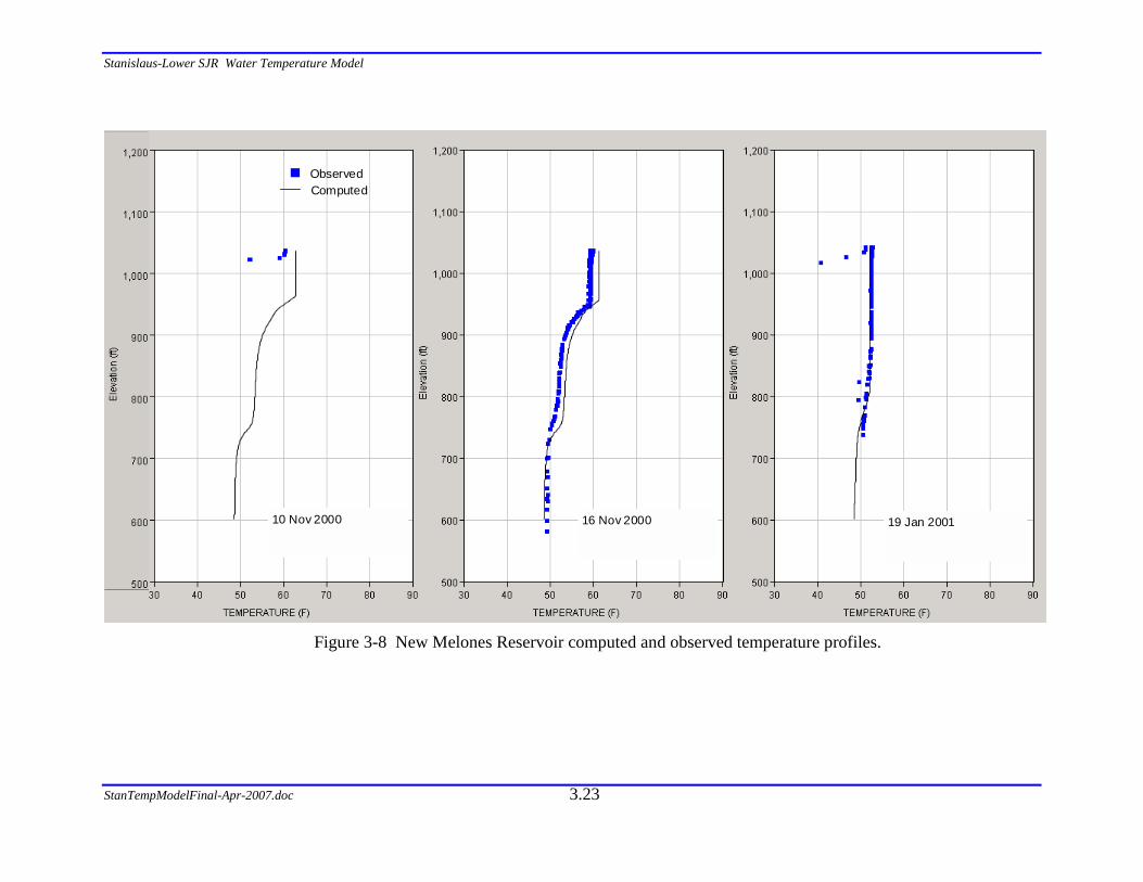
Figure 3-8 New Melones Reservoir computed and observed temperature profiles...... 3.23
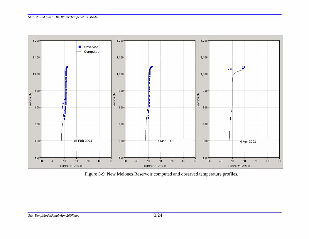
Figure 3-9 New Melones Reservoir computed and observed temperature profiles...... 3.24
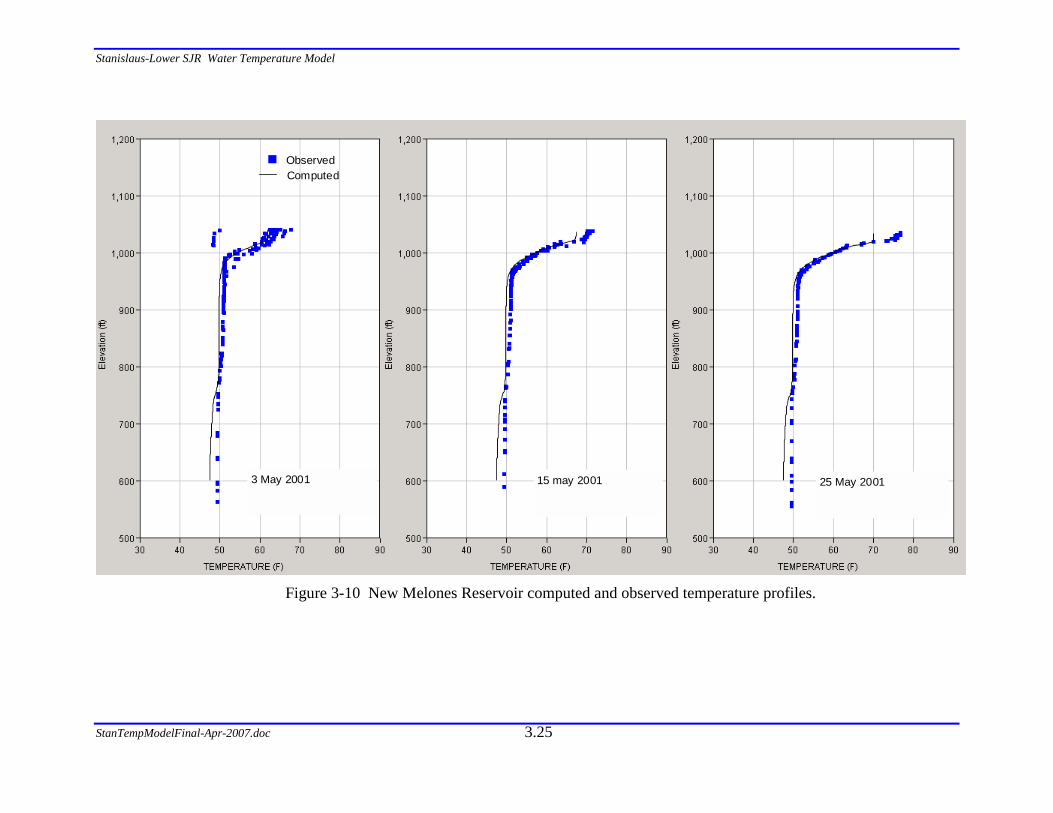
Figure 3-10 New Melones Reservoir computed and observed temperature profiles.... 3.25
Figure 3-11 New Melones Reservoir computed and observed temperature profiles.... 3.26
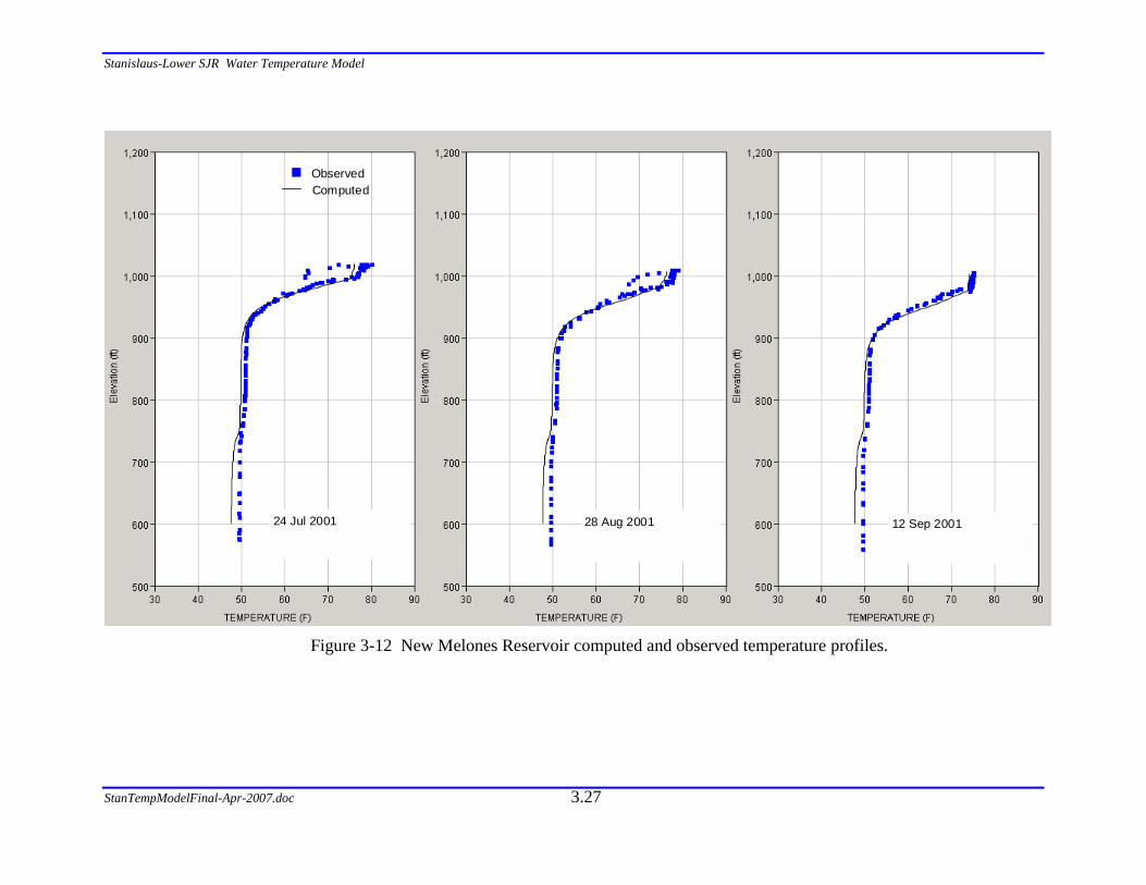
Figure 3-12 New Melones Reservoir computed and observed temperature profiles.... 3.27
Figure 3-13 New Melones Reservoir computed and observed temperature profiles.... 3.28
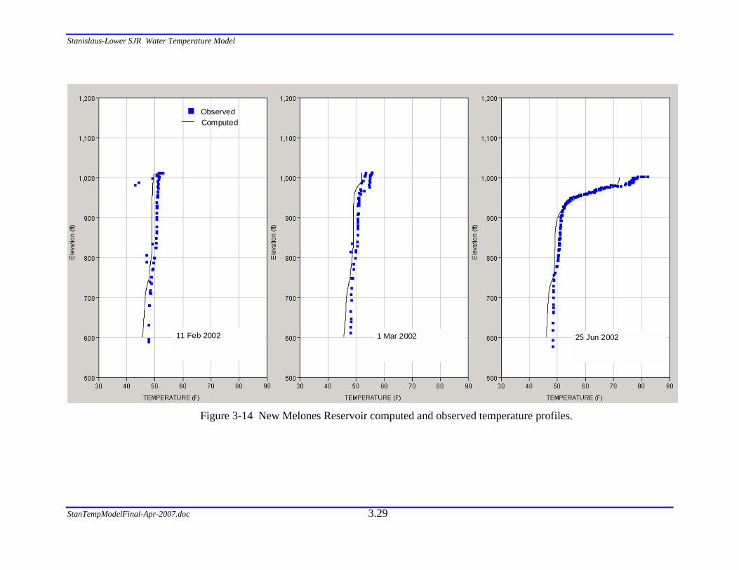
Figure 3-14 New Melones Reservoir computed and observed temperature profiles.... 3.29
Figure 3-15 New Melones Reservoir computed and observed temperature profiles.... 3.30
Figure 3-16 New Melones Reservoir computed and observed temperature profiles.... 3.31
Figure 3-17 New Melones Reservoir computed and observed temperature profiles.... 3.32
Figure 3-18 New Melones Reservoir computed and observed temperature profiles.... 3.33
Figure 3-19 New Melones Reservoir computed and observed temperature profiles.... 3.34
Figure 3-20 New Melones Reservoir computed and observed temperature profiles.... 3.35
Figure 3-21 Tulloch Reservoir computed and observed temperature profiles. ............ 3.36
Figure 3-22 Tulloch Reservoir computed and observed temperature profiles. ............ 3.37
Figure 3-23 Tulloch Reservoir computed and observed temperature profiles. ............ 3.38
Figure 3-24 Tulloch Reservoir computed and observed temperature profiles. ............ 3.39
Figure 3-25 Tulloch Reservoir computed and observed temperature profiles. ............ 3.40
Figure 3-26 Tulloch Reservoir computed and observed temperature profiles. ............ 3.41

Stanislaus-Lower SJR Water Temperature Model
StanTempModelFinal-Apr-2007.doc xi
Figure 3-27 Tulloch Reservoir computed and observed temperature profiles. ............ 3.42
Figure 3-28 Tulloch Reservoir computed and observed temperature profiles. ............ 3.43
Figure 3-29 Tulloch Reservoir computed and observed temperature profiles. ............ 3.44
Figure 3-30 Tulloch Reservoir computed and observed temperature profiles. ............ 3.45
Figure 3-31 Tulloch Reservoir computed and observed temperature profiles. ............ 3.46
Figure 3-32 Tulloch Reservoir computed and observed temperature profiles. ............ 3.47
Figure 3-33 Tulloch Reservoir computed and observed temperature profiles. ............ 3.48
Figure 3-34 Tulloch Reservoir computed and observed temperature profiles. ............ 3.49
Figure 3-35 Tulloch Reservoir computed and observed temperature profiles. ............ 3.50
Figure 3-36 Computed and observed temperature time series below Goodwin Dam. . 3-53
Figure 3-37 Computed versus observed temperatures below Goodwin Dam. ............. 3-53
Figure 3-38 Computed and observed temperature time series at Knights Ferry. ......... 3-54
Figure 3-39 Computed versus observed temperatures at Knights Ferry....................... 3-54
Figure 3-40 Computed and observed temperature time series at Orange Blossom Bridge.................................................................................................................................. 3-55
Figure 3-41 Computed versus observed temperatures at Orange Blossom Bridge. ..... 3-55
Figure 3-42 Computed and observed temperature time series at Oakdale Recreation Area. ........................................................................................................................ 3-56
Figure 3-43 Computed versus observed temperatures at Oakdale Recreation Area. ... 3-56
Figure 3-44 Computed and observed temperature time series at Riverbank Bridge. ... 3-57
Figure 3-45 Computed versus observed temperatures at Riverbank Bridge. ............... 3-57
Figure 3-46 Computed and observed temperature time series above the confluence... 3-58
Figure 3-47 Computed versus observed temperatures above the confluence............... 3-58
Figure 3-48 Computed and observed temperature time series in the San Joaquin River above the Stanislaus-San Joaquin confluence......................................................... 3-59
Figure 3-49 Computed versus observed temperatures in the San Joaquin River above the Stanislaus-San Joaquin confluence. ........................................................................ 3-59
Figure 3-50 Computed and observed temperature time series on the San Joaquin River at Patterson. ................................................................................................................. 3-60
Figure 3-51 Computed versus observed temperatures on the San Joaquin River at Patterson. ................................................................................................................. 3-60
Figure 3-52 Computed and observed temperature time series on the San Joaquin River at Durham Ferry. ......................................................................................................... 3-61
Figure 3-53 Computed versus observed temperatures on the San Joaquin River at Durham Ferry. ......................................................................................................... 3-61
Stanislaus-Lower SJR Water Temperature Model
StanTempModelFinal-Apr-2007.doc xii
Figure 4-1. Discrete criteria based on two temperatures defining three ranges of thermal conditions and associated thermal status (e.g., stress) ............................................ 4-64
Figure 4-2. Example continuous criteria based on an optimum temperature and an exponential function defining an increasingly degraded thermal condition – discrete criteria shown for comparison................................................................................. 4-64
Figure 4-3. Stanislaus River compliance locations for application of thermal criteria . 4-66
Figure 4-4. Single day and 7DADM criteria by compliance location and life stage for the September through August for the Stanislaus River ............................................... 4-67
Figure 4-5 Distribution of Instream Flow and Temperature Criteria – Districts Proposal4-70
Figure 4-6 Peer Panel Temperature Criteria Principals ................................................ 4-70
Figure 4-7 Temperature criteria for all year type proposed by the Districts ................ 4-71
Figure 4-8 Instream flow by year type proposed by CDFG ......................................... 4-72
Figure 4-9 CDFG proposal - wet year instream flow distribution................................ 4-73
Figure 4-10 CDFG proposal – above normal year instream flow distribution ............. 4-73
Figure 4-11 CDFG proposal – below normal year instream flow distribution............. 4-74
Figure 4-12 CDFG proposal – dry year instream flow distribution.............................. 4-74
Figure 4-13 CDFG proposal – critical dry year instream flow distribution ................. 4-75
Figure 4-14 Temperature criteria for wet and above normal years proposed by CDFG .. 4-76
Figure 4-15 Temperature criteria for below normal years proposed by CDFG ........... 4-77
Figure 4-16 Temperature criteria for dry and critical dry years proposed by CDFG... 4-78
Figure 4-17 New Melones storage volumes for historical, Districts and CDFG cases 4-80
Figure 4-18 New Melones water surface elevation for historical, Districts and CDFG cases ........................................................................................................................ 4-81
Figure 4-19 New Melones storage in the critical year and temperature violation with respect to the Historical Case based on the Peer Criteria, Districts Criteria, and CDFG Criteria. ........................................................................................................ 4-82
Figure 4-20 Foregone power resulting from bypassing New Melones power plant between September 15 and November 13 during years when New Melones elevation was below 900' on September 15. ........................................................................... 4-82
Figure 4-21 Evaluation of cases using Peer Criteria..................................................... 4.83
Figure 4-22 Evaluation of cases using Districts Criteria .............................................. 4.84
Figure 4-23 Evaluation of cases using CDFG Criteria ................................................. 4.85
Figure 4-24 Computed 7-day maximum and average maximum temperatures at Goodwin Dam for historical flows.......................................................................................... 4.96
Stanislaus-Lower SJR Water Temperature Model
StanTempModelFinal-Apr-2007.doc xiii
Figure 4-25 September-October 1993 New Melones outflow for base case and Tulloch re-operation alternative. .......................................................................................... 4.96
Figure 4-26 Computed 7-day average maximum temperatures at Goodwin Dam for historical (base case) and Tulloch re-operation alternative..................................... 4.97
Figure 4-27 Computed 7-day average maximum temperatures at Goodwin Dam for historical (base case) and Old Melones Dam removal alternative. ......................... 4.97
Figure 4-28 Computed 7-day average maximum temperatures at Goodwin Dam for historical (base case) and New Melones power bypass alternatives with old dam in and August, September, and May and August bypass schedules. .......................... 4.98
Figure 4-29 Computed 7-day average maximum temperatures at Goodwin Dam for historical (base case) and New Melones power bypass alternatives with old dam removed and July, August, and September bypass schedules. .............................. 4.98
Figure 4-30 Historical Flows in the SSJID/OID Joint Canal........................................ 4.99
Figure 4-31 Option 1 – Dedicated Bay (without Irrigation Outlet) ............................ 4.100
Figure 4-32 Option 2 – Shared Bay (with Irrigation Outlet) ...................................... 4.101
Figure 4-33 Computed 7-day average maximum temperatures at Goodwin Dam for historical (base case) and New Melones power bypass alternatives with August bypass schedule, with and without old dam.......................................................... 4.102
Figure 4-34 Computed 7-day average maximum temperatures at Goodwin Dam for historical (base case) and Goodwin Dam retrofit alternative. ............................... 4.102
Figure 4-35 Computed 7-day average maximum temperatures at Goodwin Dam for historical (base case) and New Melones 725’-875’ selective withdrawal alternative with old dam. Tailwater target temperatures and New Melones September power bypass alternative with old dam in are plotted for comparison. ........................... 4.103
Figure 4-36 Computed 7-day average maximum temperatures at Goodwin Dam for: Old dam removed with no other changes; New Melones 675’-875’ selective withdrawal alternative with old dam removed; and New Melones September power bypass alternative with old dam removed......................................................................... 4.103
Figure 4-37 Computed 7-day average maximum temperatures at Goodwin Dam for historical (base case), Old Melones Dam lowered 50’ with power intake lowered 100’, and power intake lowered 100’ with New Melones September power bypass................................................................................................................................ 4.104
Figure 4-38 Computed 7-day average maximum temperatures at Goodwin Dam for historical (base case), and New Melones September power bypass alternative with old dam in, with complete removal of old dam, and with partial removal of old dam................................................................................................................................ 4.104

Stanislaus-Lower SJR Water Temperature Model
StanTempModelFinal-Apr-2007.doc
1.1
1 INTRODUCTION
In the late 1990s a group of stakeholders on the Stanislaus River initiated a cooperative effort to develop a water temperature model for the Stanislaus River having recognized the need to analyze the relationship between operational alternatives, water temperature regimes and fish mortality in the Stanislaus River. These stakeholders included the U.S. Bureau of Reclamation (USBR), Fish and Wildlife Service (USFWS), California Department of Fish & Game (CDFG), Oakdale Irrigation District (OID), South San Joaquin Irrigation District (SSJID) and Stockton East Water District (SEWD). In December 1999, these partners garnered the necessary funding and through a cost sharing arrangement retained AD Consultants in association with its sub-consultant Research Management Associates, to develop the model and perform a preliminary analysis of operational alternatives. In addition, the cost-sharing partners launched an extensive program for water temperature and meteorological data collection throughout the Stanislaus River Basin, in support of the modeling effort.
In 2002, the project team presented to the stakeholders the calibrated model, results for the preliminary alternatives and a peer review report of the model prepared by Dr. Michael Deas, a consultant retained by the stakeholders to evaluate the suitability of the model its intended purpose. The stakeholders decided unanimously to accept the model and adopt it as the primary water temperature planning tool for the Stanislaus River. Nevertheless, the stakeholders recognized the need to extend the model to the Lower San Joaquin River thus enabling to study the relationship between Stanislaus operation and the temperature regime in the lower San Joaquin River as its flow to the Bay-Delta. The stakeholders also recommended that newly collected data be used to recalibrate the model. Due to lack of funding, the stakeholders decided to seek the support of CALFED for this effort through its Ecosystem Restoration Program (ERP) the stakeholders nominated Tri-Dam (Oakdale and South San Joaquin Irrigation Districts) to submit a proposal to the ERP for this project on behalf the entire Stanislaus stakeholders group.
In 2003 the project was extended to include the lower San Joaquin River through a CALFED grant (ERP-02-P28) to Tri-Dam (recipient) which is the subject of this report. A principal priority of this CALFED sponsored project was to develop a model capable of evaluating a wide range of alternatives for flow and water temperature management in the Stanislaus River and lower San Joaquin River. The work is also consistent with CALFED’s milestone 84 – “to develop water temperature management program for San Joaquin River tributaries”, and milestone 85 – “to identify thermal impacts of irrigation return flows in the San Joaquin River”. The project team was expanded and included Watercourse Engineering, Inc. and a peer review panel assigned to assist in developing temperature criteria for the evaluation of model alternatives.
The success of the project generated appreciable attention from stakeholders within other tributary basins of the San Joaquin River, especially, the Tuolumne and Merced Rivers, who have been dealing with water temperature related issues similar to

Stanislaus-Lower SJR Water Temperature Model
StanTempModelFinal-Apr-2007.doc
1.2
those on the Stanislaus River. The primary stakeholders in the Tuolumne River (Turlock Irrigation District and Modesto Irrigation District) and in the Merced River (Merced Irrigation District) basins expressed interest in adopting the same model for their own river system. Furthermore, all the stakeholders recognized the value in combining the individual models for the Stanislaus, Tuolumne and Merced Rivers into a single basin-wide model thus allowing the assessment of water operations and water temperature management scenarios in the overall San Joaquin River Basin.
In December 2004, CALFED decided to extend the Stanislaus – Lower San Joaquin River Water Temperature Model to include the Tuolumne and Merced rivers, and the main-stem San Joaquin River from Stevenson to Mossdale (to be known as the San Joaquin River (SJR) Basin-Wide Water Temperature Model). The work was to be performed in two stages: 1) Through an amendment to the existing recipient agreement with Tri-Dam (ERP-02-P28), and 2) through a two-year Directed Action, thereafter.
Under the amended scope, the recipient was to develop a beta version of the model by the end of the current agreement period (October, 2006). This work has already been accomplished, presented to CALFED and approved by a CALFED sponsored peer review (separate from the peer review panel assessing thermal criteria). The Directed Action was to allow further refinement of the model and investigate, using the model, various mechanisms for water temperature improvements both through operational and/or structural measures at existing facilities in all three tributaries of the San Joaquin River. This work commenced in October 2006.
1.1 PROJECT OBJECTIVES
The primary objective of this project was to develop an effective water temperature modeling tool for the Stanislaus River and the lower San Joaquin River.
The secondary objective was to perform detailed modeling and analysis of various alternatives for water management in the Stanislaus River basin to achieve the following:
1. Determine the relationship between water operations and river temperatures through out the Stanislaus River and San Joaquin River downstream to Mossdale.
2. Refine and validate current water temperature criteria for Central Valley fall-run Chinook salmon and Steelhead rainbow trout.
3. Simulate water operational strategies
4. Assess the merit of various water operational alternatives on water temperature.
5. Recommend a course or courses of action.
Stanislaus-Lower SJR Water Temperature Model
StanTempModelFinal-Apr-2007.doc
2.3
To achieve the identified objectives, the project team implemented the HEC-5Q model on the Stanislaus and Lower San Joaquin river system, calibrated the model, and applied the model to various investigations for water temperature improvements both through operational and/or structural measures at New Melones Reservoir, Tulloch Reservoir and Goodwin Pool. The project team analyzed the merit of those alternatives and developed a preliminary plan for the implementation of selected alternatives.
1.2 REPORT ORGANIZATION
The report is designed to provide a description of the overall work conducted under this CALFED contract (ERP-02-P28) and the necessary background needed for potential users before applying the model. The report has been divided into seven sections:
Section 1 provides an overview of the project and its objectives. Section 2 describes the HEC-5Q model and its adaptation to the Stanislaus – Lower San Joaquin river system. Section 3 presents model calibration results. Section 4 provides an overview of operations studies performed with the model including temperature objectives and alternatives analyzed. Section 5 introduces a preliminary implementation plan. Section 6 contains references cited in the report. Section 7 contains a list of attachments, including letters comments from stakeholders about this project as well as comments about water management plans proposed by other stakeholders. Section 8 describes the content of a compact disk submitted with this report, which contains this report, the model and associated input and output files.
2 MODEL DESCRIPTION
The water quality simulation module (HEC-5Q) was developed to assess temperature and a conservative water quality constituent in basin-scale planning and management decision-making. The application of HEC-5Q to the Stanislaus River and lower San Joaquin River computes the vertical or longitudinal distribution of temperature in the reservoirs and longitudinal temperature distributions in stream reaches based on daily average flows.
HEC-5Q can be used to evaluate options for coordinating reservoir releases among projects to examine the effects on flow and water quality at specified locations in the system. Example applications of the flow simulation model include examination of reservoir capacities for flood control, hydropower, and reservoir release requirements to meet water supply and irrigation demands. The model can be applied to a wide array of applications including evaluation of in-stream temperatures and several water quality constituent concentrations at critical locations in the system, examination of the potential effects of changing reservoir operations, and/or water use patterns on temperature or water quality constituent concentrations. Further, reservoir selective withdrawal operations (either existing or proposed facilities) can be simulated using HEC-5Q to determine necessary operations to meet water quality objectives downstream. This
Stanislaus-Lower SJR Water Temperature Model
StanTempModelFinal-Apr-2007.doc
2.4
option was utilized to examine a hypothetical selective withdrawal structure (TCD – temperature control device) at New Melones Dam
The HEC-5Q model used in the Stanislaus River analysis utilized only temperature and the conservative tracer (for mass continuity checking). A brief description of the processes affecting these two parameters is provided below. Refer to the HEC-5Q users manual (HEC, 2001a) for a more complete description of the water quality relationships included in model.
Temperature
The external heat sources and sinks that were considered in HEC-5Q were assumed to occur at the air-water interface, and at the sediment-water interface. Equilibrium temperature and coefficient of surface heat exchange concepts were used to evaluate the net rate of heat transfer. Equilibrium temperature is defined as the water temperature at which the net rate of heat exchange between the water surface and the overlying atmosphere is zero. The coefficient of surface heat exchange is the rate at which the heat transfer process progresses. All heat transfer mechanisms, except short-wave solar radiation, were applied at the water surface. Short-wave radiation penetrates the water surface and may affect water temperatures below the air-water interface. The depth of penetration is a function of adsorption and scattering properties of the water as affected by particulate material (i.e. phytoplankton and suspended solids). The heat exchange with the bottom is a function of conductance and the heat capacity of the bottom sediment.
Conservative parameter / tracer
The conservative parameter is unaffected by decay, settling, uptake, or other processes, and thus acts as a tracer – passively transported by advection and diffusion. This parameter was used to check mass continuity by setting the concentration of the tracer in all inflows to a constant value and then checking to ensure simulation results did reproduced the specified concentration.
2.1 MODEL REPRESENTATION OF THE PHYSICAL SYSTEM
The Stanislaus River-Lower San Joaquin River model incorporates the Stanislaus River system, including New Melones, Tulloch and Goodwin Reservoirs, a short section of the Tuolumne River extending from the San Joaquin River to Highway 99 Bridge, and the San Joaquin River from the Merced River to Mossdale.
For future work, this modeling framework has been expanded to include the Merced River system upstream of the confluence with the San Joaquin River (including McClure, McSwain, Merced Falls and Crocker-Huffman Reservoirs), and the Tuolumne River system upstream of the confluence with the San Joaquin River (including Don Pedro and La Grange Reservoirs), as well as the San Joaquin River from Stevinson near the confluence with the Merced River to Mossdale. A schematic representation of the

Stanislaus-Lower SJR Water Temperature Model
StanTempModelFinal-Apr-2007.doc
2.5
HEC-5 model of the Stanislaus system is shown in Figure 2-1, and the expanded modeling domain is shown in Figure 2-2.
Rivers and reservoirs within the Stanislaus River-Lower San Joaquin River model were represented as a network of discrete sections (reaches and/or layers, respectively) for application of HEC-5 for flow simulation, and HEC-5Q for temperature simulation. Within this network, control points (CP) were designated to represent reservoirs and selected stream locations where flow, elevations, and volumes were completed. In HEC-5, flows and other hydraulic information are computed at each control point. Within HEC-5Q, stream reaches and reservoirs were partitioned into computational elements to compute spatial variations in water temperature between control points. Within each element, uniform temperature was assumed, therefore the element size determines the spatial resolution. The model representation of reservoirs and streams is summarized in Sections 2.2 and 2.3.
Stanislaus River
Tuolum ne River
New Melones Reservoir
Tulloch Reservoir
Goodwin Reservoir
San Joaquin River
Figure 2-1 Schematic of HEC-5 model of the Stanislaus River system (shown in blue).

Stanislaus-Lower SJR Water Temperature Model
StanTempModelFinal-Apr-2007.doc
2.6
Stanislaus River
Tuolum ne River
Merced River
McClure Res ervoir
Merced Falls Reservoir
McSwain Reservoir
Crocker-Huffman Reservoir
Don Pedro Reservoir
La Grange Reservoir
New Melones Reservoir
Tulloch Reservoir
Goodwin Reservoir
San Joaquin River
Figure 2-2 Schematic of HEC-5 expanded model of the Stanislaus/Tuolumne/Merced River system.
2.2 MODEL REPRESENTATION OF RESERVOIRS
Within HEC-5Q, reservoirs can be represented as vertically or longitudinally segmented water bodies. Typically, the vertically segmented representation is applied to reservoirs that are prone to seasonal stratification, while longitudinally segmented representations are applied to impounded waters that retain riverine characteristics (e.g., a short residence time, intermittent/weak, stratification. For water quality simulations, New Melones and Tulloch Reservoirs were geometrically discretized and represented as vertically segmented water bodies with layers approximately 2 feet thick. Goodwin Reservoir was represented as vertically layered and longitudinally segmented with nine segments, and 5 layers each representing 1/5 of the cross-sectional area. Model time steps were 6-hours. A description of the different types of reservoir representation follows.

Stanislaus-Lower SJR Water Temperature Model
StanTempModelFinal-Apr-2007.doc
2.7
Vertically Segmented Reservoirs
Vertically stratified reservoirs are represented conceptually by a series of one-dimensional horizontal slices or layered volume elements, each characterized by an area, thickness, and volume. The aggregate assemblage of layered volume elements is a geometrically discretized representation of the prototype reservoir. The geometric characteristics of each horizontal slice are defined as a function of the reservoir’s area-capacity curve. Within each horizontal layer (or ‘element’) of a vertically segmented reservoir, the water is assumed to be fully mixed with all isopleths parallel to the water surface both laterally and longitudinally. External inflows and withdrawals occur as sources or sinks within each element and are instantaneously dispersed and homogeneously mixed throughout the layer from the headwaters of the impoundment to the dam. Consequently, simulation results are most representative of conditions in the main reservoir body and may not accurately describe flow or quality characteristics in shallow regions or near reservoir banks. It is not possible to model longitudinal variations in water quality constituents using the vertically segmented configuration.
The allocation of the inflow to individual elements is based on the relative densities of the inflow and the reservoir elements. Flow entrainment is considered as the inflowing water seeks a depth or level of similar density.
Vertical advection is one of two transport mechanisms used in HEC-5Q to simulate transport of water quality constituents between elements in a vertically segmented reservoir. Vertical transport is defined as the inter-element flow that results in flow continuity. An additional transport mechanism used to distribute water quality constituents between elements is effective diffusion, representing the combined effects of molecular and turbulent diffusion, and convective mixing or the physical movement of water due to density instability. Wind and flow-induced turbulent diffusion and convective mixing are the dominant components of effective diffusion in the epilimnion of most reservoirs.
The outflow component of the model incorporates a selective withdrawal technique for withdrawal through multiple dam outlet or other submerged orifices, or for flow over a weir. The relationships developed for the ‘WES Withdrawal Allocation Method’ describe the vertical limits of the withdrawal zone and the vertical velocity distribution throughout the water column.
For the Stanislaus River application, the existing conditions incorporated into HEC-5Q include:
1) New Melones power intake (elevation 775 feet at top of intake pipe) is always utilized for water surface elevations greater than 786.5 feet. The low-level outlet (two pipes) operates at lake elevations less than 786.5 feet. New Melones Spillway has never been used although it would be if releases greater than 7,700 cfs occurred.
2) Tulloch low-level (power intake) is always used except for flows greater than 2,060 cfs. Excess flows are passes through the gated spillway.
For New Melones bypass alternative simulations, power flows are bypassed to the low-level outlet to access deeper, cooler lake water. For operational alternative simulations, New Melones Dam is operated with selective withdrawal capability.
Stanislaus-Lower SJR Water Temperature Model
StanTempModelFinal-Apr-2007.doc
2.8
Longitudinally Segmented Reservoirs
Longitudinally segmented reservoirs are represented conceptually as a linear network of a specified number of segments or volume elements. The length of a segment, coupled with an associated stage-width relationship, characterize the geometry of each reservoir segment. Surface areas, volumes and cross-sectional areas are computed from the width relationship.
Additionally, longitudinally segmented reservoirs can be subdivided into vertical elements, with each element assumed fully mixed in the vertical and lateral directions. Branching of reservoirs is allowed. For reservoirs represented as layered and longitudinally segmented, all cross-sections contain the same number of layers and each layer is assigned the same fraction of the reservoir cross-sectional area. Therefore, the thickness of each element varies with the width versus elevation relationship for each element. The model performs a backwater computation to define the water surface profile as a function of the hydraulic gradient based on flow and Manning’s equation.
A uniform vertical flow distribution is specified at the upstream end of each reservoir. Velocity profiles within the body of the reservoir may be calculated as flow over a submerged weir or as a function of a downstream density profile. Linear interpolation is performed for reservoir segments without specifically defined flow fields.
External flows, such as withdrawals and tributary inflows, occur as sinks or sources within the segment. Inflows to the upstream ends of reservoir branches are allocated to individual elements in proportion to the fraction of the cross-section assigned to each layer. Other inflows to the reservoir are distributed in proportion to the local reservoir flow distribution. External flows may be allocated along the length of the reservoir to represent dispersed non-point source inflows such as agricultural drainage and groundwater accretions.
Vertical variations in constituent concentrations can be computed for the layered and longitudinally segmented reservoir model. Mass transport between vertical layers is represented by net flow determined by mass balance and by diffusion.
Vertical flow distributions at dams are based on weir or orifice withdrawal. The velocity distribution within the water column is calculated as a function of the water density and depth using the WES weir withdrawal or orifice withdrawal allocation method
Goodwin Dam currently has no low-level outlet. The seasonally warmer surfaces waters are thus preferentially released to the river (over the spillway, elevation 359 feet) and deeper, cooler water is diverted to the two water districts. The Goodwin retrofit plan, discussed below, incorporates a low-level siphon to access the deeper, cooler waters for release downstream
2.2.1 New Melones Reservoir
New Melones Reservoir is a large impoundment that is subject to strong seasonal stratification. Of special interest are the representation of New Melones Reservoir and, in
Stanislaus-Lower SJR Water Temperature Model
StanTempModelFinal-Apr-2007.doc
2.9
particular, the impacts of the old dam on the flow and thermal regime of the reservoir and the reservoir release temperatures.
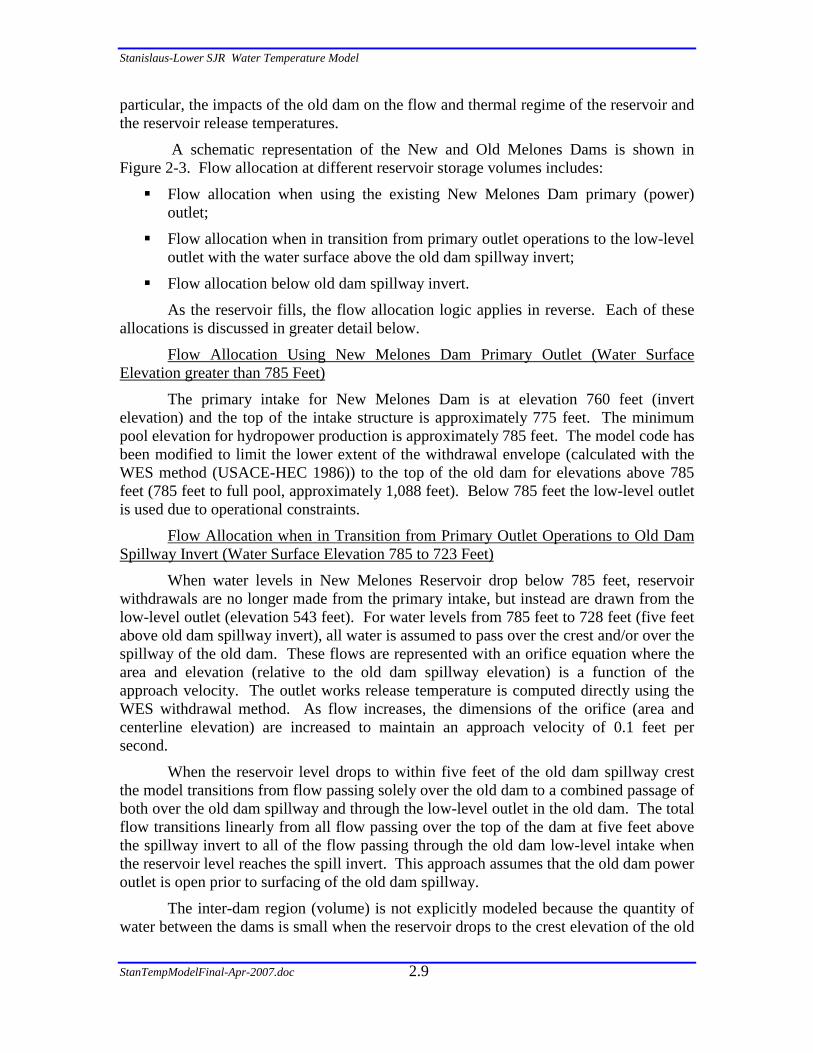
A schematic representation of the New and Old Melones Dams is shown in Figure 2-3. Flow allocation at different reservoir storage volumes includes:
! Flow allocation when using the existing New Melones Dam primary (power) outlet;
! Flow allocation when in transition from primary outlet operations to the low-level outlet with the water surface above the old dam spillway invert;
! Flow allocation below old dam spillway invert.
As the reservoir fills, the flow allocation logic applies in reverse. Each of these allocations is discussed in greater detail below.
Flow Allocation Using New Melones Dam Primary Outlet (Water Surface Elevation greater than 785 Feet)
The primary intake for New Melones Dam is at elevation 760 feet (invert elevation) and the top of the intake structure is approximately 775 feet. The minimum pool elevation for hydropower production is approximately 785 feet. The model code has been modified to limit the lower extent of the withdrawal envelope (calculated with the WES method (USACE-HEC 1986)) to the top of the old dam for elevations above 785 feet (785 feet to full pool, approximately 1,088 feet). Below 785 feet the low-level outlet is used due to operational constraints.
Flow Allocation when in Transition from Primary Outlet Operations to Old Dam Spillway Invert (Water Surface Elevation 785 to 723 Feet)
When water levels in New Melones Reservoir drop below 785 feet, reservoir withdrawals are no longer made from the primary intake, but instead are drawn from the low-level outlet (elevation 543 feet). For water levels from 785 feet to 728 feet (five feet above old dam spillway invert), all water is assumed to pass over the crest and/or over the spillway of the old dam. These flows are represented with an orifice equation where the area and elevation (relative to the old dam spillway elevation) is a function of the approach velocity. The outlet works release temperature is computed directly using the WES withdrawal method. As flow increases, the dimensions of the orifice (area and centerline elevation) are increased to maintain an approach velocity of 0.1 feet per second.
When the reservoir level drops to within five feet of the old dam spillway crest the model transitions from flow passing solely over the old dam to a combined passage of both over the old dam spillway and through the low-level outlet in the old dam. The total flow transitions linearly from all flow passing over the top of the dam at five feet above the spillway invert to all of the flow passing through the old dam low-level intake when the reservoir level reaches the spill invert. This approach assumes that the old dam power outlet is open prior to surfacing of the old dam spillway.
The inter-dam region (volume) is not explicitly modeled because the quantity of water between the dams is small when the reservoir drops to the crest elevation of the old

Stanislaus-Lower SJR Water Temperature Model
StanTempModelFinal-Apr-2007.doc
2.10
dam (approximately 2,400 acre-feet). If the reservoir is stratified during the transition period, warm waters flow over the top of the old dam and cooler waters flow through the low-level intake. The New Melones Reservoir release temperature is calculated using a mass balance: water that passes over the dam and that which passes through the low-level intake are assumed mixed completely and instantaneously in proportion to their total quantity.
Flow Allocation Below Old Dam Spillway Invert (Water Surface Elevation less than 723 feet)
Once below the old dam spillway invert, all flows are passed through the low-level outlet and assigned a withdrawal envelope according to the WES withdrawal approach (USACE-HEC 1986) and the physical characteristics of the old dam power intake.
Figure 2-3 Schematic representation of New and Old Melones Dams
Spillway El. 1088
Crest El. 1135
Min. Power Pool El. 785Intake El. 760
Crest El. 735Spillway El. 723
El. 543
El. 610
Transition Zone: 3-4 feet
New DamOld Dam
Not to Scale
Vol. 2,400 AF
Stanislaus-Lower SJR Water Temperature Model
StanTempModelFinal-Apr-2007.doc
2.11
2.3 MODEL REPRESENTATION OF STREAMS
In HEC-5Q, river or stream reaches are represented conceptually as a linear network of segments or volume elements. The length, width, cross-sectional area and a flow versus depth relationship characterize each element. Cross-sections are defined at all control points and at intermediate locations where data are available. The flow versus depth relation is developed external to HEC-5Q using available cross-section data and appropriate hydraulic computations. Linear interpolation between input cross-section locations is used to define the hydraulic data for each element.
For the Stanislaus River, three river reaches are modeled: upstream of New Melones Reservoir, between New Melones Dam and Tulloch Reservoir, and from Goodwin Dam to the confluence with the San Joaquin River. Upstream of New Melones Reservoir, a short river reach is modeled, wherein the modeled length is a function of New Melones elevation. This variable length allows heat exchange in the normally inundated old river channel to be simulated. Downstream of New Melones, Corp of Engineers cross-sections, field reconnaissance, and aerial photographs were used to define the geometry of the stream reaches. A total of 83 cross sections were utilized to define the river geometry.
San Joaquin River reaches include: Merced River confluence to the Tuolumne River confluence, Tuolumne River confluence to Stanislaus River confluence, and Stanislaus River confluence to Old River. A short reach of the Tuolumne River is included in the model, from the Highway 99 Bridge to the confluence with the San Joaquin River
Flow rates are calculated at stream control points by HEC-5 using one of several available hydrologic routing methods. For this project, all flows were routed using specified routing that explicitly defines travel time between control points. Within HEC-5, incremental local flows (i.e., flow between adjacent control points such as inflows or withdrawals may include any point or non-point flow) are assumed to enter at the control point. Within HEC-5Q, incremental local flow for a particular reach may be divided into components and placed at different locations within the stream reach (i.e., that portion of the stream bounded by the two control points). The diversions (demands) are allocated to individual control points within the river reaches or reservoirs. Distributed flows such as groundwater accretions and non-specific agricultural return flows are defined on a rate per mile basis. A flow balance is used to determine the flow rate at element boundaries.
For simulation of water quality (e.g., temperature), the tributary locations and associated water quality are specified (see subsequent section). To allocate components of the diversion flow balance, HEC-5Q performs a calculation using any specified withdrawals, inflows, or return flows, and distributes the balance uniformly along the stream reach. Once inter-element flows are established, the water depth, surface width and cross sectional area are computed at each element boundary, assuming normal flow and downstream control (i.e., backwater). For this study, there were no return flows other than groundwater. Stream elements were approximately one mile long. The river elements above New Melones varied with reservoir stage, expanding in length under low
Stanislaus-Lower SJR Water Temperature Model
StanTempModelFinal-Apr-2007.doc
2.12
storage conditions and contracting at high storage levels. Consistent with the reservoir representation, model time steps were 6-hours in length.
2.4 HYDROLOGIC & TEMPERATURE BOUNDARY CONDITIONS
HEC-5Q requires that flow rates and water quality be defined for all inflows. Daily data from USGS and the California Department of Water Resources (DWR) California Data Exchange Center (CDEC), as well as the United States Bureau of Reclamation (USBR) reservoir operation data provided the daily flow data used to develop all hydrologic boundary flows. Inflow rates may be defined explicitly or as a fraction of the incremental local flow to the control point as defined by HEC-5. Table 2-1 lists fractions of the net incremental inflow assigned to each of the individual tributaries to New Melones Reservoir (net inflow equals the total inflow minus Stanislaus and Collierville PH flows). Remaining system inflows are also included in Table 2-1 with data source or method used for their computation. The incremental accretion/depletion to the San Joaquin River was computed by mass balance of USGS gauge data and allocated to nine separate locations.
Tributary stream inflow temperature relationships were developed from observed hourly CDEC and project data for the period of 1999 through 2005. These data were analyzed and two types of inflow relationships were developed, which were then used to define temperatures for all years at 6-hour intervals. For the Stanislaus powerhouse, there is a consistent seasonality observed in the data, so inflow temperatures were based solely on the day of the year. For other major inflows, a composite relationship was developed that considered meteorology (equilibrium temperature), flow rate, and a seasonal temperature distribution. The seasonal temperatures were defined to represent high flow conditions (e.g., elevated flows due to snow melt and dam releases). At high flows, there was a seasonal bias. At lower flows, there was an equilibrium temperature bias. Flow rate also influenced the diurnal variation with a large range of inflow temperatures at lower flows and shallower water depths. The temperatures of stream accretions were assumed equal to the ambient stream temperature. Very limited small stream/return flow temperature data suggests that this is a reasonable approximation; however, the current data collection effort may provide sufficient data to further refine this approximation.

Stanislaus-Lower SJR Water Temperature Model
StanTempModelFinal-Apr-2007.doc
2.13
Table 2-1 Incremental inflow assignment.
Tributary Data Source / Computation Method Stanislaus PH above New Melones USGS gauge data Collierville PH above New Melones USGS gauge data Middle + North Forks above New Melones Computed (60% of net inflow to New Melones*) South Fork above New Melones Computed (25% of net inflow to New Melones*) Other inflows to New Melones Computed (15% of net inflow to New Melones*) Inflows to Tulloch Computed (mass balance on Tulloch) South San Joaquin Canal spill Computed (Ripon flow-Goodwin release) San Joaquin River at Newman USGS gauge data Tuolumne River at Modesto USGS gauge data Incremental San Joaquin inflow Computed (Tuolumne+San Joaquin @ Newman +
Ripon flow – San Joaquin @ Vernalis) *Net inflow to New Melones = total inflow – Stanislaus and Collierville PH flows
2.5 METEOROLOGICAL DATA
For temperature simulation using HEC-5Q, specification of water surface heat exchange data requires designation of meteorological zones within the study area. Each control point within the system or sub-system used in temperature or water quality simulation must be associated with a defined meteorological zone. Meteorological zones represent hourly data from the Modesto California Irrigation Management Information System (CIMIS) station for the period of 1989 - 2005.
Meteorological data for the 1980 – 1988 period were developed by extrapolation of the CIMIS data based on daily National Weather Service (NWS) maximum and minimum air temperature data for Modesto. The relationship between the maximum and minimum air temperatures of the CIMIS and NWS data were developed by comparing data for each day that air temperatures were available (1989–2002). For each day when CIMIS data were unavailable, the NWS temperature extremes were adjusted using the relationship described above and then the hourly CIMIS data that best replicated the NWS extreme was selected for use in the model. The CIMIS records considered were limited to within 2 days before or after the calendar day, thus up to 5 days from each of the 17 years (1989-2005) of CIMIS data (a maximum of 85 days) were considered.
Hourly air temperature, wind speed, relative humidity, and cloud cover for each day is used to compute the average equilibrium temperature, surface heat exchange rate, solar radiation flux and wind speed at 6-hour intervals for input to HEC-5Q. Solar radiation and wind speed are used in the reservoir simulation to attenuate solar energy below the water surface and to compute wind induced turbulent mixing parameters.
Stanislaus-Lower SJR Water Temperature Model
StanTempModelFinal-Apr-2007.doc
3.14
Three meteorological zones were used in the Stanislaus River model. Heat exchange coefficients for each zone were computed to reflect typical environmental conditions. For sheltered stream sections, wind speed was reduced and shading was assumed to reflect riparian canopy conditions. Reduced wind speed decreases the evaporative heat loss and results in higher equilibrium temperatures and lower heat exchange rates. Shading reduces solar radiation resulting in lower equilibrium temperatures and lower heat exchange rates. No riparian shading was assumed for reservoirs and for the lower San Joaquin River. For New Melones and Tulloch Reservoirs the wind speed was increased to reflect open water conditions.
The meteorological data collected as part of this project were used in determining the heat exchange adjustments to the individual stream sections.
3 MODEL CALIBRATION
The HEC-5Q model of the Stanislaus River system was previously calibrated to 1990 –1999 data. The current effort involves refinement of the initial calibration based on additional data available for the five year period from 2000 through 2004, including reservoir temperature profile observations in New Melones Reservoir, Tulloch Reservoir, and Goodwin Reservoir, as well as temperature time series observations at several stations in the Stanislaus River and Lower San Joaquin River (see Section 7.1). Minor adjustments have been made to model coefficients during the current calibration; however, previous calibration results remain relevant representations of model performance.
The following California Department of Fish and Game (CDFG) reservoir profile data sets, and CDEC and USGS time series data sets for the 2000 – 2004 calibration period were utilized. A map of these locations is shown in Figure 3-1.
• Temperature profile data in New Melones Reservoir (CDFG).
• Temperature profile data in Tulloch Reservoir (CDFG).
• Temperature time series data below Goodwin Dam (USGS).
• Temperature time series data at Knights Ferry, Orange Blossom Bridge, Oakdale Recreation Area, Riverbank Bridge, and above the confluence with the San Joaquin River (CDEC).
• Temperature time series data at Ripon (USGS).
• Temperature time series data on the San Joaquin River at Patterson and Durham Ferry (CDFG/CDEC).
The hydrology, meteorology, and inflow water quality conditions described in Chapter 2 were assumed.
The intent of model calibration exercise was to minimize the differences between the computed and observed data, and demonstrate that the model adequately represents the thermal responses of the prototype stream and reservoir system. The final water
Stanislaus-Lower SJR Water Temperature Model
StanTempModelFinal-Apr-2007.doc
3.15
quality coefficients of the calibrated models are listed on the model output CD that accompanies this report.
The results of the calibration effort are presented as plots of computed versus observed values using various formats. The final results of the calibration effort may be viewed using the graphical user interface (GUI). The GUI is described in Exhibit 4 of the HEC-5Q Users Guide. The following sections provide a brief discussion of the calibration results for reservoirs and streams. Station locations are shown in Figure 3-1. The following discussion proceeds by data set as listed above.
3.1 RESERVOIR TEMPERATURE CALIBRATION RESULTS
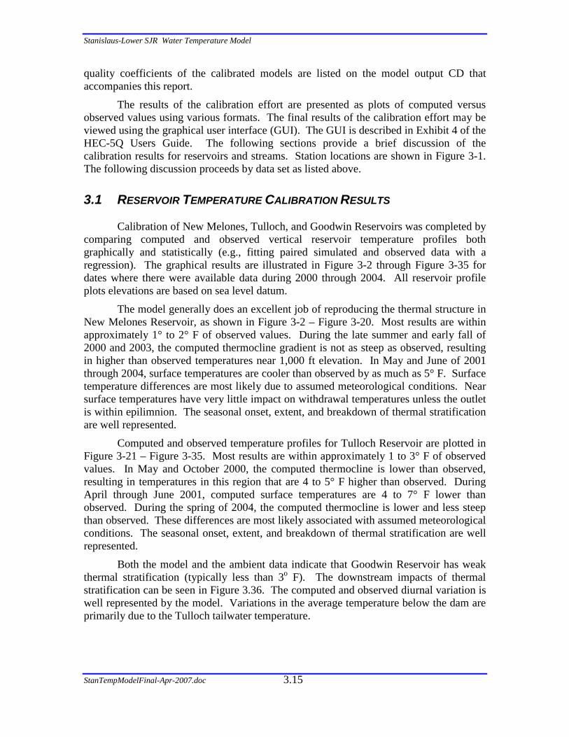
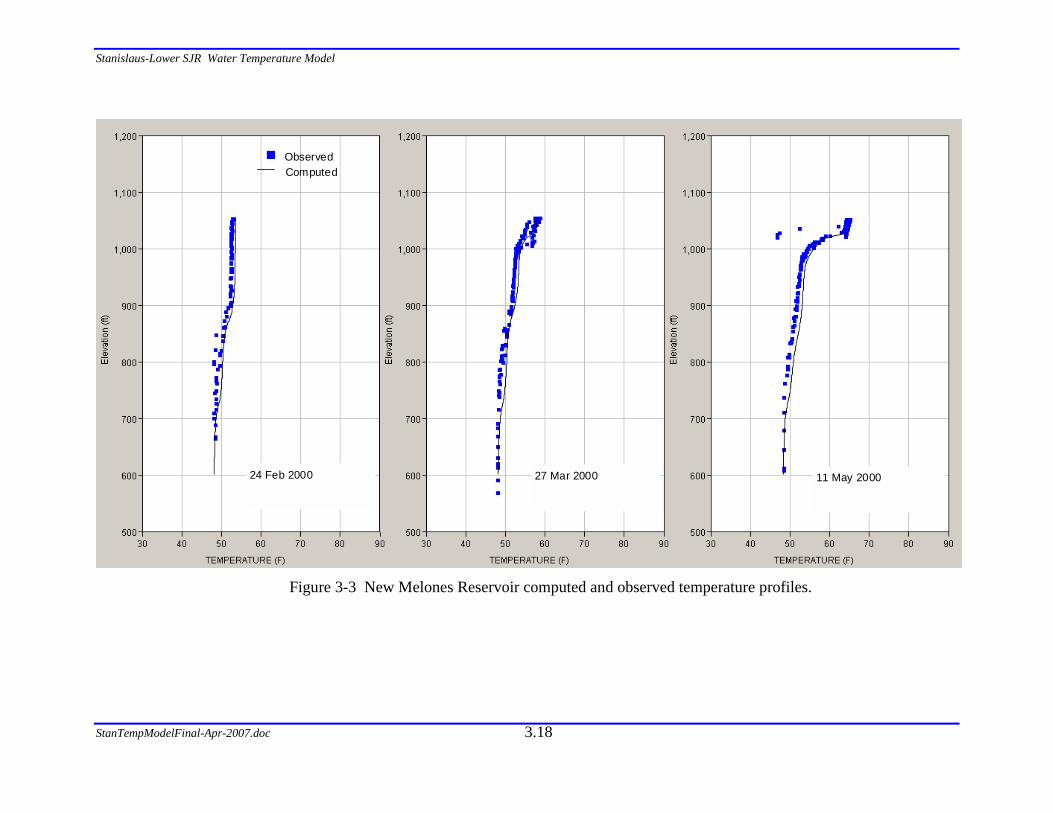
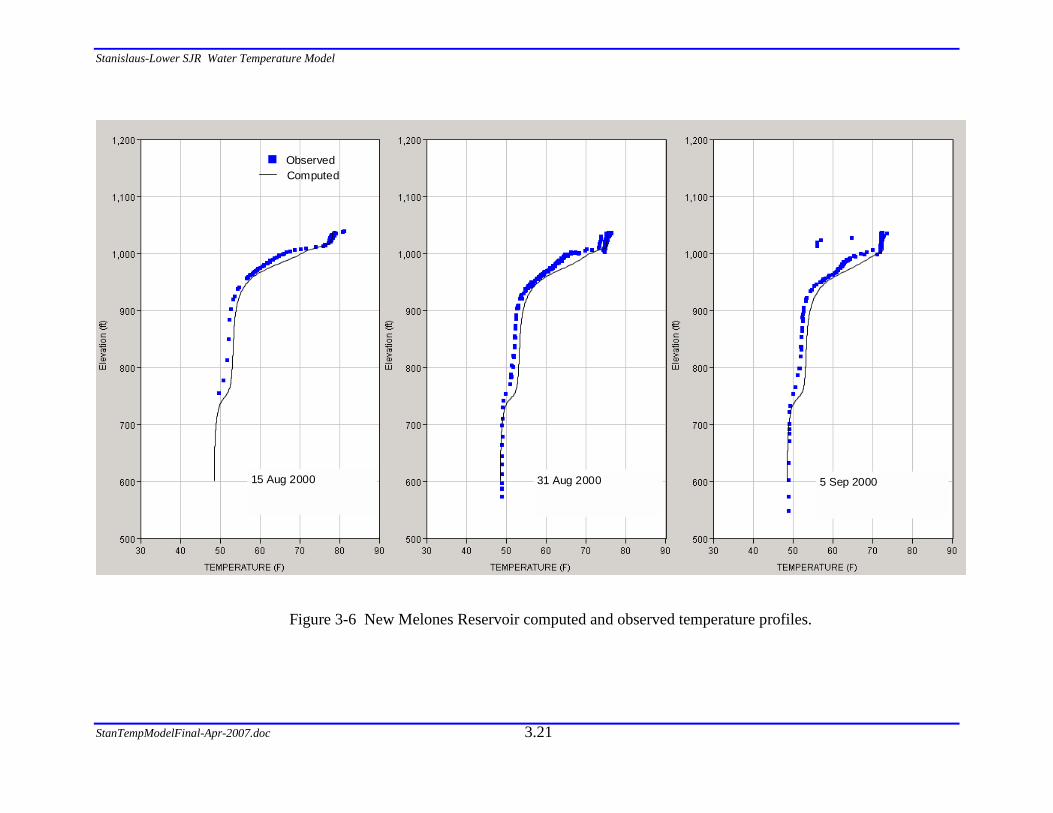
Calibration of New Melones, Tulloch, and Goodwin Reservoirs was completed by comparing computed and observed vertical reservoir temperature profiles both graphically and statistically (e.g., fitting paired simulated and observed data with a regression). The graphical results are illustrated in Figure 3-2 through Figure 3-35 for dates where there were available data during 2000 through 2004. All reservoir profile plots elevations are based on sea level datum.
The model generally does an excellent job of reproducing the thermal structure in New Melones Reservoir, as shown in Figure 3-2 – Figure 3-20. Most results are within approximately 1° to 2° F of observed values. During the late summer and early fall of 2000 and 2003, the computed thermocline gradient is not as steep as observed, resulting in higher than observed temperatures near 1,000 ft elevation. In May and June of 2001 through 2004, surface temperatures are cooler than observed by as much as 5° F. Surface temperature differences are most likely due to assumed meteorological conditions. Near surface temperatures have very little impact on withdrawal temperatures unless the outlet is within epilimnion. The seasonal onset, extent, and breakdown of thermal stratification are well represented.
Computed and observed temperature profiles for Tulloch Reservoir are plotted in Figure 3-21 – Figure 3-35. Most results are within approximately 1 to 3° F of observed values. In May and October 2000, the computed thermocline is lower than observed, resulting in temperatures in this region that are 4 to 5° F higher than observed. During April through June 2001, computed surface temperatures are 4 to 7° F lower than observed. During the spring of 2004, the computed thermocline is lower and less steep than observed. These differences are most likely associated with assumed meteorological conditions. The seasonal onset, extent, and breakdown of thermal stratification are well represented.
Both the model and the ambient data indicate that Goodwin Reservoir has weak thermal stratification (typically less than 3o F). The downstream impacts of thermal stratification can be seen in Figure 3.36. The computed and observed diurnal variation is well represented by the model. Variations in the average temperature below the dam are primarily due to the Tulloch tailwater temperature.

Stanislaus-Lower SJR Water Temperature Model
StanTempModelFinal-Apr-2007.doc
3.16
Stanislaus River
Tuolumne River
New Melones Reservoir
Tulloch Reservoir
Goodw in Reservoir
San Joaquin River
Knights Ferry
Ripon
Orange Blossom Bridge
Durham Ferry
Patterson
Riverbank Bridge
Oakdale Rec. Area
Figure 3-1 Locations for 2000 – 2004 calibration plots.

Stanislaus-Lower SJR Water Temperature Model
StanTempModelFinal-Apr-2007.doc
3.17
Observed Computed
4 Jan 2000 28 Jan 2000 10 Jan 2000
Figure 3-2 New Melones Reservoir computed and observed temperature profiles.
Stanislaus-Lower SJR Water Temperature Model
StanTempModelFinal-Apr-2007.doc
3.18
Observed Computed
24 Feb 2000 11 May 2000 27 Mar 2000
Figure 3-3 New Melones Reservoir computed and observed temperature profiles.

Stanislaus-Lower SJR Water Temperature Model
StanTempModelFinal-Apr-2007.doc
3.19
Observed Computed
16 May 2000 11 Jul 2000 7 Jun 2000
Figure 3-4 New Melones Reservoir computed and observed temperature profiles.

Stanislaus-Lower SJR Water Temperature Model
StanTempModelFinal-Apr-2007.doc
3.20
Observed Computed
20 Jul 2000 11 Aug 2000 2 Aug 2000
Figure 3-5 New Melones Reservoir computed and observed temperature profiles.
Stanislaus-Lower SJR Water Temperature Model
StanTempModelFinal-Apr-2007.doc
3.21
Observed Computed
15 Aug 2000 5 Sep 2000 31 Aug 2000
Figure 3-6 New Melones Reservoir computed and observed temperature profiles.
Stanislaus-Lower SJR Water Temperature Model
StanTempModelFinal-Apr-2007.doc
3.22
Observed Computed
15 Sep 2000 16 Oct 2000 26 Sep 2000
Figure 3-7 New Melones Reservoir computed and observed temperature profiles.
Stanislaus-Lower SJR Water Temperature Model
StanTempModelFinal-Apr-2007.doc
3.23
Observed Computed
10 Nov 2000 19 Jan 2001 16 Nov 2000
Figure 3-8 New Melones Reservoir computed and observed temperature profiles.
Stanislaus-Lower SJR Water Temperature Model
StanTempModelFinal-Apr-2007.doc
3.24
Observed Computed
15 Feb 2001 4 Apr 2001 7 Mar 2001
Figure 3-9 New Melones Reservoir computed and observed temperature profiles.
Stanislaus-Lower SJR Water Temperature Model
StanTempModelFinal-Apr-2007.doc
3.25
Observed Computed
3 May 2001 25 May 2001 15 may 2001
Figure 3-10 New Melones Reservoir computed and observed temperature profiles.

Stanislaus-Lower SJR Water Temperature Model
StanTempModelFinal-Apr-2007.doc
3.26
Observed Computed
5 Jun 2001 13 Jul 2001 28 Jun 2001
Figure 3-11 New Melones Reservoir computed and observed temperature profiles.
Stanislaus-Lower SJR Water Temperature Model
StanTempModelFinal-Apr-2007.doc
3.27
Observed Computed
24 Jul 2001 12 Sep 2001 28 Aug 2001
Figure 3-12 New Melones Reservoir computed and observed temperature profiles.

Stanislaus-Lower SJR Water Temperature Model
StanTempModelFinal-Apr-2007.doc
3.28
Observed Computed
4 Oct 2001 9 Jan 2002 19 Nov 2001
Figure 3-13 New Melones Reservoir computed and observed temperature profiles.
Stanislaus-Lower SJR Water Temperature Model
StanTempModelFinal-Apr-2007.doc
3.29
Observed Computed
11 Feb 2002 25 Jun 2002 1 Mar 2002
Figure 3-14 New Melones Reservoir computed and observed temperature profiles.
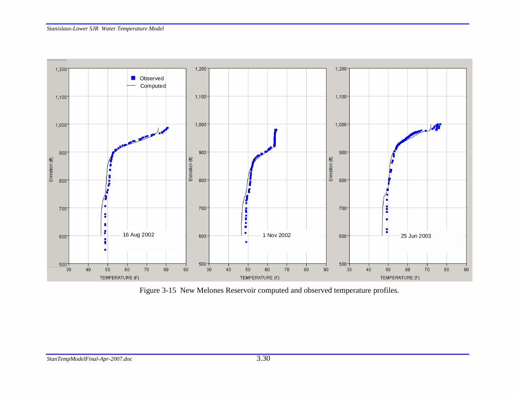
Stanislaus-Lower SJR Water Temperature Model
StanTempModelFinal-Apr-2007.doc
3.30
Observed Computed
16 Aug 2002 25 Jun 2003 1 Nov 2002
Figure 3-15 New Melones Reservoir computed and observed temperature profiles.

Stanislaus-Lower SJR Water Temperature Model
StanTempModelFinal-Apr-2007.doc
3.31
Observed Computed
31 Jul 2003 24 Sep 2003 29 Aug 2003
Figure 3-16 New Melones Reservoir computed and observed temperature profiles.
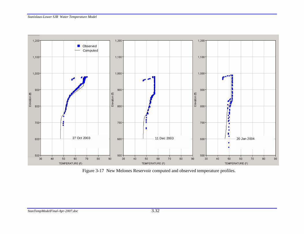
Stanislaus-Lower SJR Water Temperature Model
StanTempModelFinal-Apr-2007.doc
3.32
Observed Computed
27 Oct 2003 20 Jan 2004 11 Dec 2003
Figure 3-17 New Melones Reservoir computed and observed temperature profiles.
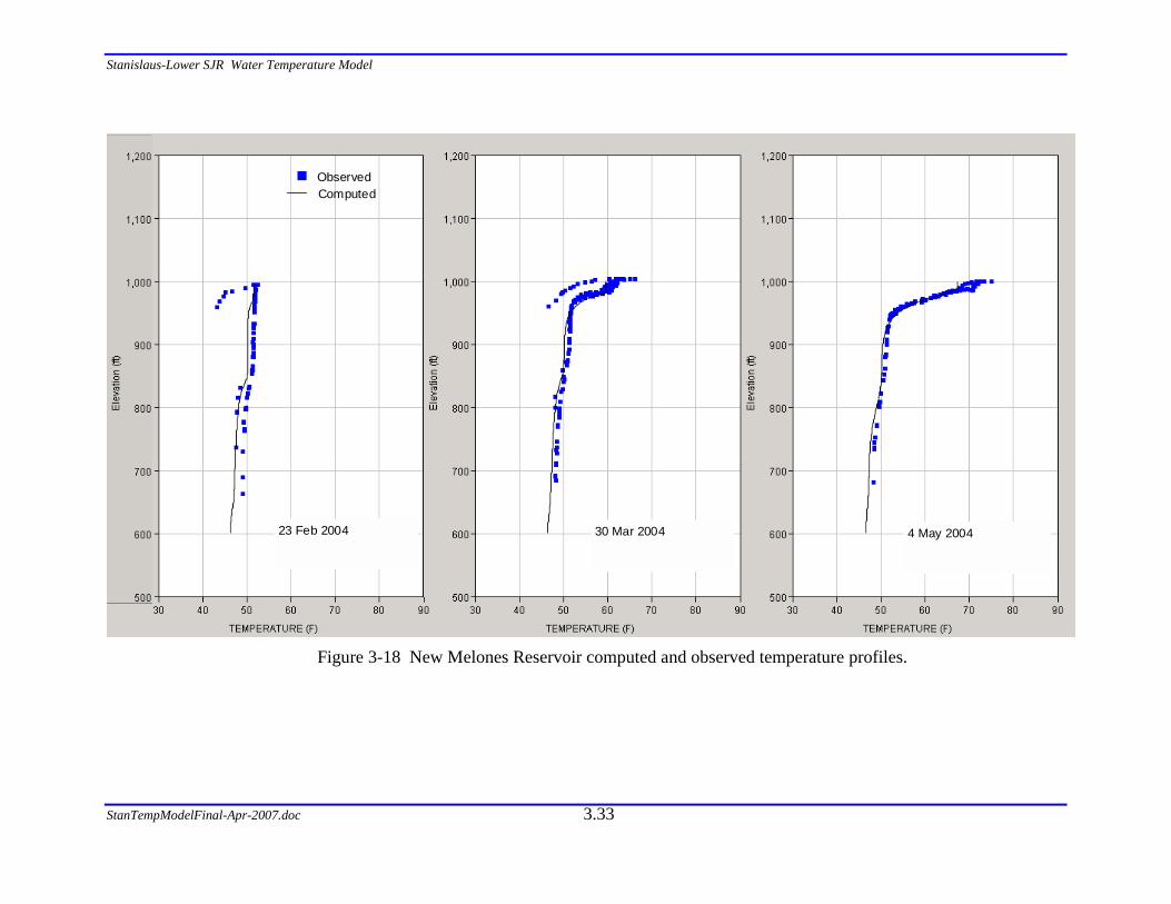
Stanislaus-Lower SJR Water Temperature Model
StanTempModelFinal-Apr-2007.doc
3.33
Observed Computed
23 Feb 2004 4 May 2004 30 Mar 2004
Figure 3-18 New Melones Reservoir computed and observed temperature profiles.

Stanislaus-Lower SJR Water Temperature Model
StanTempModelFinal-Apr-2007.doc
3.34
Observed Computed
27 May 2004 19 Jul 2004 22 Jun 2004
Figure 3-19 New Melones Reservoir computed and observed temperature profiles.
Stanislaus-Lower SJR Water Temperature Model
StanTempModelFinal-Apr-2007.doc
3.35
Observed Computed
17 Aug 2004 15 Oct 2004 20 Sep 2004
Figure 3-20 New Melones Reservoir computed and observed temperature profiles.

Stanislaus-Lower SJR Water Temperature Model
StanTempModelFinal-Apr-2007.doc
3.36
Observed Computed
4 Jan 2000 7 Jun 2000 16 May 2000
Figure 3-21 Tulloch Reservoir computed and observed temperature profiles.

Stanislaus-Lower SJR Water Temperature Model
StanTempModelFinal-Apr-2007.doc
3.37
Observed Computed
11 Jul 2000 2 Aug 2000 20 Jul 2000
Figure 3-22 Tulloch Reservoir computed and observed temperature profiles.

Stanislaus-Lower SJR Water Temperature Model
StanTempModelFinal-Apr-2007.doc
3.38
Observed Computed
15 Aug 2000 26 Sep 2000 5 Sep 2000
Figure 3-23 Tulloch Reservoir computed and observed temperature profiles.
Stanislaus-Lower SJR Water Temperature Model
StanTempModelFinal-Apr-2007.doc
3.39
Observed Computed
16 Oct 2000 19 Jan 2000 8 Dec 2000
Figure 3-24 Tulloch Reservoir computed and observed temperature profiles.

Stanislaus-Lower SJR Water Temperature Model
StanTempModelFinal-Apr-2007.doc
3.40
Observed Computed
15 Feb 2001 25 Apr 2001 24 Apr 2001
Figure 3-25 Tulloch Reservoir computed and observed temperature profiles.

Stanislaus-Lower SJR Water Temperature Model
StanTempModelFinal-Apr-2007.doc
3.41
Observed Computed
15 May 2001 28 Jun 2001 5 Jun 2001
Figure 3-26 Tulloch Reservoir computed and observed temperature profiles.
Stanislaus-Lower SJR Water Temperature Model
StanTempModelFinal-Apr-2007.doc
3.42
Observed Computed
13 Jul 2001 28 Aug 2001 24 Jul 2001
Figure 3-27 Tulloch Reservoir computed and observed temperature profiles.
Stanislaus-Lower SJR Water Temperature Model
StanTempModelFinal-Apr-2007.doc
3.43
Observed Computed
12 Sep 2001 19 Nov 2001 4 Oct 2001
Figure 3-28 Tulloch Reservoir computed and observed temperature profiles.
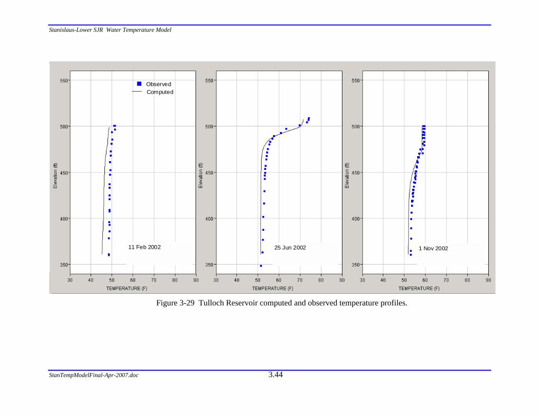
Stanislaus-Lower SJR Water Temperature Model
StanTempModelFinal-Apr-2007.doc
3.44
Observed Computed
11 Feb 2002 1 Nov 2002 25 Jun 2002
Figure 3-29 Tulloch Reservoir computed and observed temperature profiles.

Stanislaus-Lower SJR Water Temperature Model
StanTempModelFinal-Apr-2007.doc
3.45
Observed Computed
25 Jun 2003 29 Aug 2003 18 Jul 2003
Figure 3-30 Tulloch Reservoir computed and observed temperature profiles.
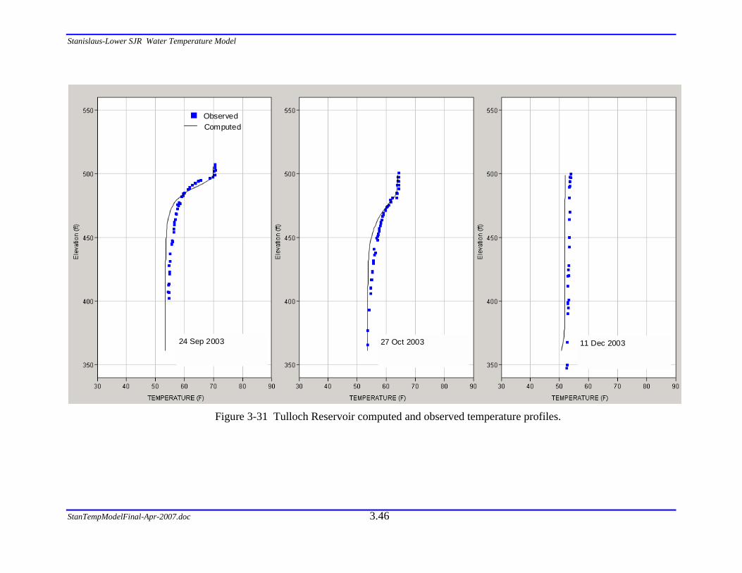
Stanislaus-Lower SJR Water Temperature Model
StanTempModelFinal-Apr-2007.doc
3.46
Observed Computed
24 Sep 2003 11 Dec 2003 27 Oct 2003
Figure 3-31 Tulloch Reservoir computed and observed temperature profiles.

Stanislaus-Lower SJR Water Temperature Model
StanTempModelFinal-Apr-2007.doc
3.47
Observed Computed
20 Jan 2004 23 Mar 2004 23 Feb 2004
Figure 3-32 Tulloch Reservoir computed and observed temperature profiles.
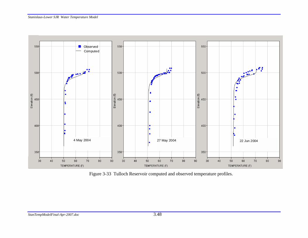
Stanislaus-Lower SJR Water Temperature Model
StanTempModelFinal-Apr-2007.doc
3.48
Observed Computed
4 May 2004 22 Jun 2004 27 May 2004
Figure 3-33 Tulloch Reservoir computed and observed temperature profiles.

Stanislaus-Lower SJR Water Temperature Model
StanTempModelFinal-Apr-2007.doc
3.49
Observed Computed
19 Jul 2004 20 Sep 2004 17 Aug 2004
Figure 3-34 Tulloch Reservoir computed and observed temperature profiles.

Stanislaus-Lower SJR Water Temperature Model
StanTempModelFinal-Apr-2007.doc
3.50
Observed Computed
17 Aug 2004 15 Oct 2004 20 Sep 2004
Figure 3-35 Tulloch Reservoir computed and observed temperature profiles.
Stanislaus-Lower SJR Water Temperature Model
StanTempModelFinal-Apr-2007.doc
3-51
3.2 STREAM TEMPERATURE CALIBRATION RESULTS
Calibration of the Stanislaus River was completed by comparing computed and observed time series temperatures both graphically and statistically (e.g., fitting paired simulated and observed data with a regression). Six locations along the Stanislaus River were employed: Knights Ferry, Orange Blossom Bridge, Oakdale Recreation Area, Riverbank Bridge, Ripon, and at the confluence of the Stanislaus and San Joaquin Rivers. The graphical results are illustrated in Figure 3-36 through Figure 3-53 for 2000 through 2004. The time series plots show that an excellent representation of the average temperatures, diurnal variation, and daily and season variation is achieved at each location.
In the computed versus observed temperature plots, an exact match between computed and observed data would result in an equation with a slope of 1 and an intercept of 0, or y = 1x + 0, and an R2 coefficient of determination value of 1. Discrepancies between computed and observed data result in non-zero intercept values and slopes greater than or less than 1. Differences between data points and the line described by the equation result in an R2 value less than 1. Line equations for the best linear fit to the data are shown on each computed versus observed plot. Mean values for X (computed) and Y (observed) are also shown on these plots.
R2 values are generally about 0.9 at all locations except below Goodwin Dam (Figure 3-36 and Figure 3-37). At this location, computed temperatures are overall lower than observed data as seen in Figure x. The discrepancy between computed and observed data results in an R2 value of 0.85, and the smallest slope (0.75) and largest intercept (14.4) of all the best linear fit equations.
Table 3-1 summarizes the 2000 through 2004 results for each location. The averages of the observed and computed values used in the computed versus observed plots are listed, along with the coefficient of determination (R2 value).
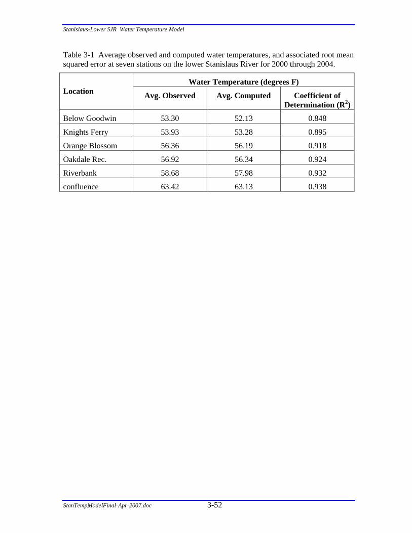
Stanislaus-Lower SJR Water Temperature Model
StanTempModelFinal-Apr-2007.doc 3-52
Table 3-1 Average observed and computed water temperatures, and associated root mean squared error at seven stations on the lower Stanislaus River for 2000 through 2004.
Water Temperature (degrees F) Location Avg. Observed Avg. Computed Coefficient of
Determination (R2)
Below Goodwin 53.30 52.13 0.848
Knights Ferry 53.93 53.28 0.895
Orange Blossom 56.36 56.19 0.918
Oakdale Rec. 56.92 56.34 0.924
Riverbank 58.68 57.98 0.932
confluence 63.42 63.13 0.938

Stanislaus-Lower SJR Water Temperature Model
StanTempModelFinal-Apr-2007.doc 3-53
Computed
Observed
Figure 3-36 Computed and observed temperature time series below Goodwin Dam.
R2 = 0.848 Y = 0.746*X+14.403
Computed Vs. Observed
Figure 3-37 Computed versus observed temperatures below Goodwin Dam.

Stanislaus-Lower SJR Water Temperature Model
StanTempModelFinal-Apr-2007.doc 3-54
Computed
Observed
Figure 3-38 Computed and observed temperature time series at Knights Ferry.
R2 = 0.895 Y = 0.817*X+10.412
Computed Vs. Observed
Figure 3-39 Computed versus observed temperatures at Knights Ferry.

Stanislaus-Lower SJR Water Temperature Model
StanTempModelFinal-Apr-2007.doc 3-55
Computed
Observed
Figure 3-40 Computed and observed temperature time series at Orange Blossom Bridge.
R2 = 0.918 Y = 0.801*X+11.343
Computed Vs. Observed
Figure 3-41 Computed versus observed temperatures at Orange Blossom Bridge.

Stanislaus-Lower SJR Water Temperature Model
StanTempModelFinal-Apr-2007.doc 3-56
Computed
Observed
Figure 3-42 Computed and observed temperature time series at Oakdale Recreation
Area.
R2 = 0.924 Y = 0.785*X+12.696
Computed Vs. Observed
Figure 3-43 Computed versus observed temperatures at Oakdale Recreation Area.
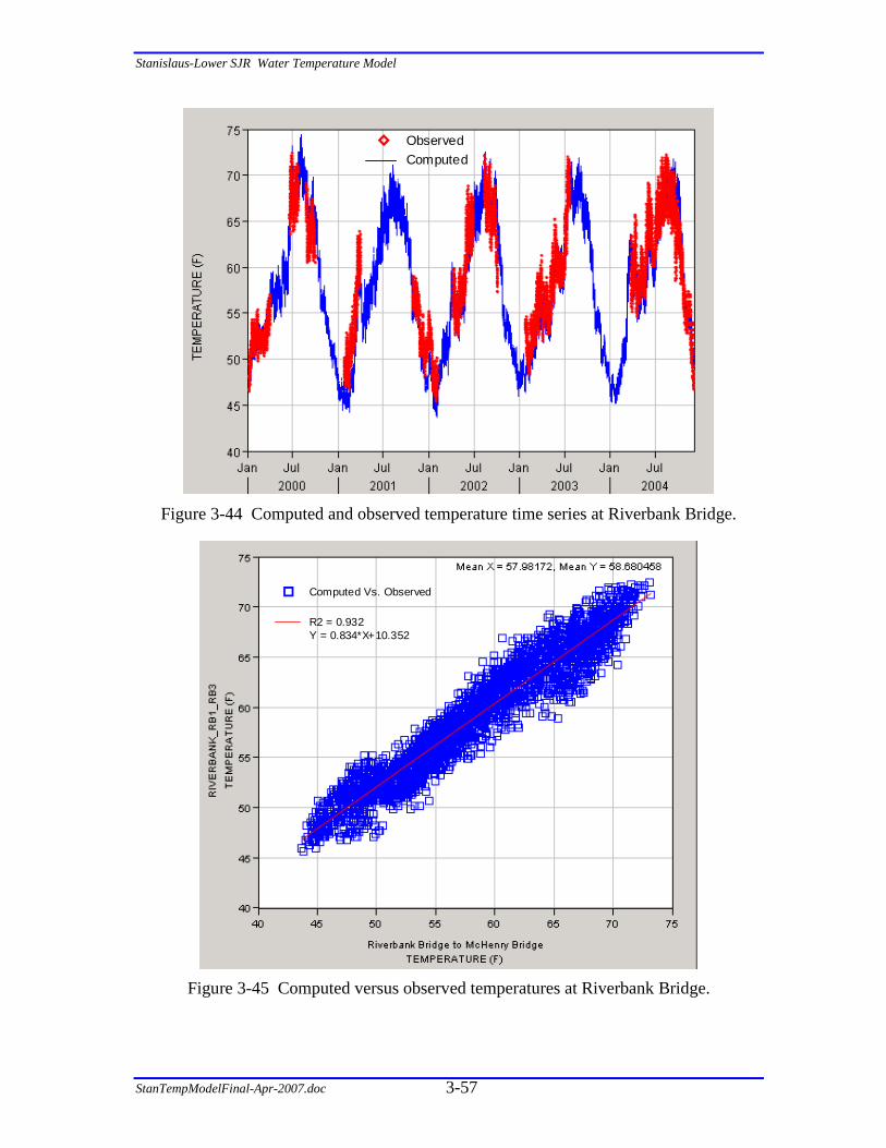
Stanislaus-Lower SJR Water Temperature Model
StanTempModelFinal-Apr-2007.doc 3-57
Computed Observed
Figure 3-44 Computed and observed temperature time series at Riverbank Bridge.
R2 = 0.932 Y = 0.834*X+10.352
Computed Vs. Observed
Figure 3-45 Computed versus observed temperatures at Riverbank Bridge.

Stanislaus-Lower SJR Water Temperature Model
StanTempModelFinal-Apr-2007.doc 3-58
Computed Observed
Figure 3-46 Computed and observed temperature time series above the confluence.
R2 = 0.938 Y = 0.906*X+6.249
Computed Vs. Observed
Figure 3-47 Computed versus observed temperatures above the confluence.

Stanislaus-Lower SJR Water Temperature Model
StanTempModelFinal-Apr-2007.doc 3-59
Computed Observed
Figure 3-48 Computed and observed temperature time series in the San Joaquin River
above the Stanislaus-San Joaquin confluence.
R2 = 0.957 Y = 0.899*X+6.374
Computed Vs. Observed
Figure 3-49 Computed versus observed temperatures in the San Joaquin River above the
Stanislaus-San Joaquin confluence.
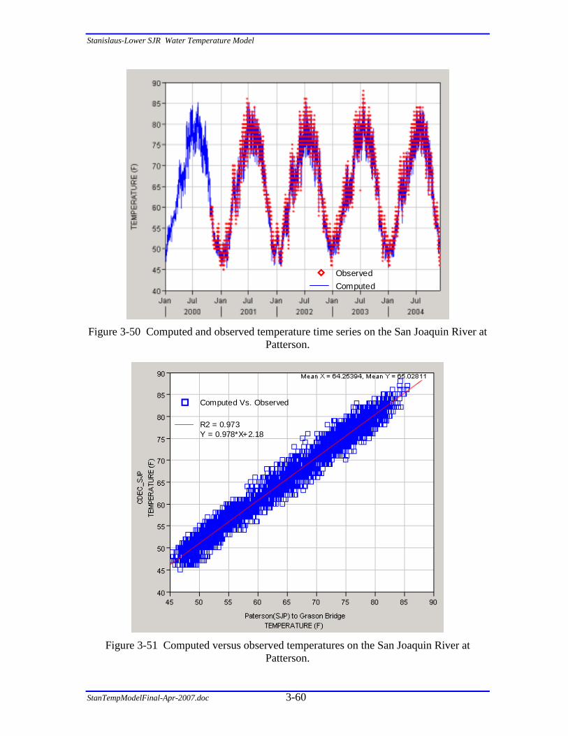
Stanislaus-Lower SJR Water Temperature Model
StanTempModelFinal-Apr-2007.doc 3-60
Computed Observed
Figure 3-50 Computed and observed temperature time series on the San Joaquin River at
Patterson.
R2 = 0.973 Y = 0.978*X+2.18
Computed Vs. Observed
Figure 3-51 Computed versus observed temperatures on the San Joaquin River at
Patterson.
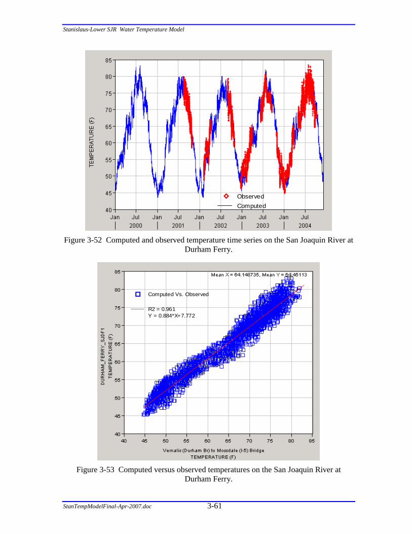
Stanislaus-Lower SJR Water Temperature Model
StanTempModelFinal-Apr-2007.doc 3-61
Computed Observed
Figure 3-52 Computed and observed temperature time series on the San Joaquin River at
Durham Ferry.
R2 = 0.961 Y = 0.884*X+7.772
Computed Vs. Observed
Figure 3-53 Computed versus observed temperatures on the San Joaquin River at
Durham Ferry.
Stanislaus-Lower SJR Water Temperature Model
StanTempModelFinal-Apr-2007.doc 4-62
4 OPERATIONS STUDY
4.1 INTRODUCTION
The purpose of the Operations Study was to investigate various mechanisms for water temperature improvements in the Stanislaus River both through operational and/or structural measures at New Melones Reservoir, Tulloch Reservoir and Goodwin Pool.
The model simulated various alternatives of Stanislaus River operation. The alternatives consisted of two categories: (1) Water Management Plans for re-operation of New Melones proposed by the irrigation districts and fishery agencies, and (2) Other Operational and Physical Changes in the system that were developed jointly by the Stanislaus stakeholders and/or initiated by the project team.
For the Water management Plans, the model estimated the temperature response at specified control points on the river, and the effect on water supply and storage at New Melones Reservoir. The driving force behind those proposals is the desire to meet water temperature objectives at defined control points in the river system that would enhance habitat conditions for fall-run Chinook salmon and Steelhead rainbow trout.
The temperature objectives (or criteria) were developed by a panel of experts (Peer Review Panel), as discussed in the following section. It should be emphasized that the stakeholders agreed that the Peer criteria should only serve as a means for comparing simulated alternatives and should not be construed as an agreed upon criteria in establishing temperature policy in the basin. Furthermore, the Peer Panel recommended that stakeholders should build upon and/or modify the Peer criteria given their own on-the-ground experience and knowledge of fishery issues related to the Stanislaus and Lower San-Joaquin river system.
For the Other Operational and Physical Changes, the model estimated the temperature impact in absolute terms by examining specific time periods and system conditions when those changes are most relevant.
4.2 TEMPERATURE OBJECTIVES
One of several inter-related tasks in the San Joaquin River Water Temperature Modeling and Analysis project was the need to review and assess available information to identify water temperature criteria for fall-run Chinook salmon and steelhead. A peer review panel (Panel) was assembled to evaluate the biological merits, and application of thermal criteria in assessment of model generated alternatives for the Stanislaus River. Three independent scientific experts who have a history of leadership activities and who have a demonstrated ability to deal with complex issues in a balanced manner:
• John Bartholow, United States Geological Survey
• Chuck Hanson, Hanson Environmental
• Chris Myrick, Colorado State University

Stanislaus-Lower SJR Water Temperature Model
StanTempModelFinal-Apr-2007.doc 4-63
This group included scientists with local expertise, relevant discipline knowledge, as well as experience outside the Delta or Bay-Delta water issues. The panel was chaired by Mike Deas, Principal at Watercourse Engineering, Inc. Outlined herein is a brief summary of the Panel findings. Specific details on development of the thermal criteria are presented in Deas et al (2004) (see Section 7.2), wherein the complete Panel charge, discussion of existing criteria, assessment of alternative criteria, presentation of technical information supporting the Panel thermal criteria, and other relevant information are presented.
In sum, thermal criteria were developed for various life stages (e.g., adult migration, egg incubation, juvenile rearing) of anadromous fish based on 7-day average of the maximum daily temperatures (7DADM). Panel members identified optimum threshold temperatures after EPA (2003): a well-documented source, with specific identified processes and procedures, and extensive peer review. These values were intended to be a common starting point for assessment of thermal criteria. Further, the Panel felt that local resource managers should adapt the criteria as necessary when assessing model-simulated alternatives if there was supporting evidence to refine the criteria for the Stanislaus River.
4.2.1 Framework
A critical Panel conclusion was that a two threshold (e.g., optimal, suboptimal, and lethal ranges) criteria did not necessarily differentiate alternatives on a broad scale. Further, from the outset of this review, the Panel had concerns over the discontinuous format of the two threshold (three-range) criteria - specifically, the inability of the discrete ranges to represent the continuous physiological response of a particular life stage. An example of how discontinuous criteria represent thermal conditions is provided in Figure 4-1. Temperatures Ta, Tb, and Tc, represent conditions in the high sub-optimal range, the low sub-optimal range, and in the optimal range, respectively. Note in this discrete representation, thermal condition (e.g., stress) is equivalent for Ta and Tb, and markedly greater than Tc even though Tb and Tc are nearly equivalent temperatures.

Stanislaus-Lower SJR Water Temperature Model
StanTempModelFinal-Apr-2007.doc 4-64
Tem
pera
ture
Tem
pera
ture
Thermal Status (e.g., stress)
Sub-optimal
Lethal
Optimal
a
b
Ta
Tb
a
bcc
Ta
Tb Tc Tc
Figure 4-1. Discrete criteria based on two temperatures defining three ranges of
thermal conditions and associated thermal status (e.g., stress)
To overcome these discrete ranges the panel elected to modify the two threshold (three range) criteria and adopt a response function that would essentially allow a continuous representation of increasingly adverse thermal conditions (Figure 4-2). In this case thermal status is more representative of a continual, but exponentially increasing function with increasing temperature, with thermal status at Tb markedly lower than at Ta, but only marginally higher than Tc.
Tem
pera
ture
Tem
pera
ture
a
b
Ta
Tb
a
bc c
Ta
Tb Tc Tc
Thermal Status (e.g., stress) Figure 4-2. Example continuous criteria based on an optimum temperature and an
exponential function defining an increasingly degraded thermal condition – discrete criteria shown for comparison
Construction of the temperature response curves shown above, were identified for each life stage based on an exponential relationship. Complete details are presented in Deas et al (2004).
Stanislaus-Lower SJR Water Temperature Model
StanTempModelFinal-Apr-2007.doc 4-65
In addition to the weekly average criteria, single day maximum temperatures were also considered because short duration elevated temperature events (on the order of a few hours) can have profound impacts on anadromous fish populations. Thus, an additional metric representing a one-day instantaneous maximum lethal water temperature was developed based on an upper incipient lethal condition. This criterion defined incipient upper lethal temperatures (IULT) as a thermal condition that would result in severe impairment to the fish when exposed for a short duration (hours). The application of this daily instantaneous maximum criteria/metric was to identify short duration events that are potentially masked by the 7DADM temperature. In the early fall or late spring, when thermal conditions are generally changing most rapidly, sub-weekly conditions may be highly variable and can put fish under stress. A modeled alternative that produced many instantaneous daily maximum temperatures above the selected criteria would indicate potential short-term impacts and the single day maximum criteria may assist in assessing alternatives, i.e., this criterion is intended to raise a “red flag” versus a quantitative measure.
4.2.2 Application
Compliance or reference points where the criteria for the various life stages are applied were subsequently identified with Stakeholder input. Compliance points for the Stanislaus River include:
- Orange Blossom Bridge [River Mile RM 46] (summer juvenile rearing) - Riverbank [RM 33] (juvenile rearing and egg incubation) - Confluence with the San Joaquin [RM 0] (smoltification and adult immigration)
Additional compliance points of interest included Goodwin Dam [RM 57.9], Knights Ferry [RM 54], Oakdale [RM 40], and Ripon [RM 15]. Compliance points may move with season and life stage and may not include all locations listed. These locations are shown in Figure 4-3. Single day criteria were applied at the same locations as the 7DADM. An example of the single day and 7DADM criteria by compliance location and life stage for the September through August period is shown in Figure 4-4.
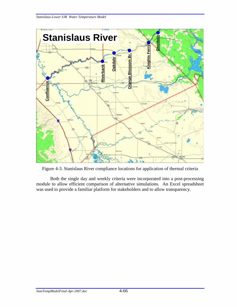
Stanislaus-Lower SJR Water Temperature Model
StanTempModelFinal-Apr-2007.doc 4-66
Goo
dwin
Oak
dale
Riv
erba
nk
Stanislaus RiverC
onflu
ence
Kni
ghts
Fer
ry
Ora
nge
Blo
ssom
Br.
Figure 4-3. Stanislaus River compliance locations for application of thermal criteria
Both the single day and weekly criteria were incorporated into a post-processing module to allow efficient comparison of alternative simulations. An Excel spreadsheet was used to provide a familiar platform for stakeholders and to allow transparency.
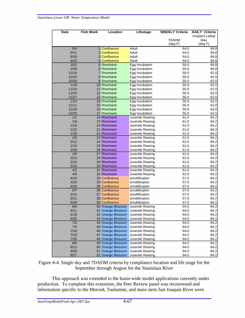
Stanislaus-Lower SJR Water Temperature Model
StanTempModelFinal-Apr-2007.doc 4-67
Date Fish Week Location Lifestage WEEKLY Criteria DAILY Criteria
7DADMIncipient Lethal
Max(deg F) (deg F)
9/4 1 Confluence Adult 64.0 69.89/11 2 Confluence Adult 64.0 69.89/18 3 Confluence Adult 64.0 69.89/25 4 Confluence Adult 64.0 69.810/2 5 Riverbank Egg Incubation 55.0 69.810/9 6 Riverbank Egg Incubation 55.0 69.8
10/16 7 Riverbank Egg Incubation 55.0 62.010/23 8 Riverbank Egg Incubation 55.0 62.010/30 9 Riverbank Egg Incubation 55.0 62.011/6 10 Riverbank Egg Incubation 55.0 62.0
11/13 11 Riverbank Egg Incubation 55.0 62.011/20 12 Riverbank Egg Incubation 55.0 62.011/27 13 Riverbank Egg Incubation 55.0 62.012/4 14 Riverbank Egg Incubation 55.0 62.0
12/11 15 Riverbank Egg Incubation 55.0 62.012/18 16 Riverbank Egg Incubation 55.0 62.012/25 17 Riverbank Egg Incubation 55.0 62.0
1/1 18 Riverbank Juvenile Rearing 61.0 84.21/8 19 Riverbank Juvenile Rearing 61.0 84.2
1/15 20 Riverbank Juvenile Rearing 61.0 84.21/22 21 Riverbank Juvenile Rearing 61.0 84.21/29 22 Riverbank Juvenile Rearing 61.0 84.22/5 23 Riverbank Juvenile Rearing 61.0 84.2
2/12 24 Riverbank Juvenile Rearing 61.0 84.22/19 25 Riverbank Juvenile Rearing 61.0 84.22/26 26 Riverbank Juvenile Rearing 61.0 84.23/5 27 Riverbank Juvenile Rearing 61.0 84.2
3/12 28 Riverbank Juvenile Rearing 61.0 84.23/19 29 Riverbank Juvenile Rearing 61.0 84.23/26 30 Riverbank Juvenile Rearing 61.0 84.24/2 31 Riverbank Juvenile Rearing 61.0 84.24/9 32 Riverbank Juvenile Rearing 61.0 84.2
4/16 33 Confluence smoltification 57.0 84.24/23 34 Confluence smoltification 57.0 84.24/30 35 Confluence smoltification 57.0 84.25/7 36 Confluence smoltification 57.0 84.2
5/14 37 Confluence smoltification 57.0 84.25/21 38 Confluence smoltification 57.0 84.25/28 39 Confluence smoltification 57.0 84.26/4 40 Orange Blossom Juvenile Rearing 64.0 84.2
6/11 41 Orange Blossom Juvenile Rearing 64.0 84.26/18 42 Orange Blossom Juvenile Rearing 64.0 84.26/25 43 Orange Blossom Juvenile Rearing 64.0 84.27/2 44 Orange Blossom Juvenile Rearing 64.0 84.27/9 45 Orange Blossom Juvenile Rearing 64.0 84.2
7/16 46 Orange Blossom Juvenile Rearing 64.0 84.27/23 47 Orange Blossom Juvenile Rearing 64.0 84.27/30 48 Orange Blossom Juvenile Rearing 64.0 84.28/6 49 Orange Blossom Juvenile Rearing 64.0 84.2
8/13 50 Orange Blossom Juvenile Rearing 64.0 84.28/20 51 Orange Blossom Juvenile Rearing 64.0 84.28/27 52 Orange Blossom Juvenile Rearing 64.0 84.2
Figure 4-4. Single day and 7DADM criteria by compliance location and life stage for the September through August for the Stanislaus River
This approach was extended to the basin-wide model applications currently under production. To complete this extension, the Peer Review panel was reconvened and information specific to the Merced, Tuolumne, and main stem San Joaquin River were
Stanislaus-Lower SJR Water Temperature Model
StanTempModelFinal-Apr-2007.doc 4-68
reviewed in light of application of identified thermal criteria on the Stanislaus River. The Peer Review panel identified that the methodology applied on the Stanislaus River was appropriate for the additional river reaches.
For the Peer Review Panel findings for the Stanislaus River and for the larger basin application (external to the Stanislaus River) see Section 7.2. For initial comments by Tuolumne and Merced stakeholders regarding temperature criteria applicable to their individual river basins, see Section 7.4. These comments will be address as part of the model extension in next phase of the project.
4.3 ALTERNATIVES
The alternatives consist of operational changes, physical changes of existing facilities and combinations of the two. The alternatives studied with the model were divided into two categories:
1) Water Management Plans – these are operational options consisting of diversions and instream flow schedules proposed by stakeholders, primarily, the water irrigation districts and the fishery agencies.
2) Other Operational and Physical Changes – these are other concepts that were developed through discussions with the stakeholders or initiated by the project team. These concepts are stand-alone options and, if feasible, could be implemented in conjunction with the Water Management Plans.
It should be noted that the irrigation districts and the fisheries agencies requested that their view on each other’s proposals be included in this report. References to the files containing these comments letters are included in Section 7.3.1 and 7.3.2 as follows:
7.3.1 Irrigation Districts (OID, SSJID, SEWD & Tri-Dam) Comments:
• TEMPERATURE.M102306.MODELING.pdf
• Memo121306final.pdf 7.3.2 California Department of Fish and Game Comments:
• DraftSRTempModelRpt_CDFGLetter.pdf
• FinalRptCDFGCommentLetter040907.pdf
4.3.1 Water Management Plans
The water management options were developed by the Stanislaus Stakeholders through a series of workshops with the participation of representatives from irrigation districts (Districts) and fishery agencies (CDFG). Water management plans consisted of three common elements:
1) Proposed diversions schedules
2) Proposed instream flow schedules
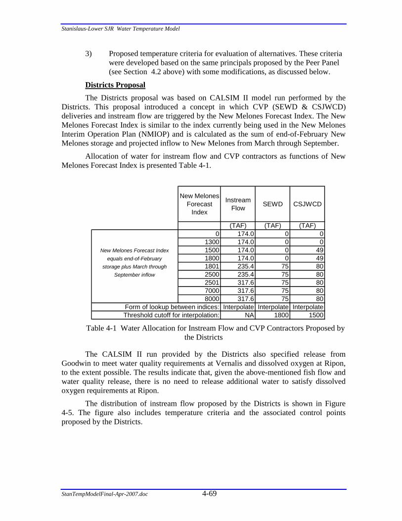
Stanislaus-Lower SJR Water Temperature Model
StanTempModelFinal-Apr-2007.doc 4-69
3) Proposed temperature criteria for evaluation of alternatives. These criteria were developed based on the same principals proposed by the Peer Panel (see Section 4.2 above) with some modifications, as discussed below.
Districts Proposal The Districts proposal was based on CALSIM II model run performed by the
Districts. This proposal introduced a concept in which CVP (SEWD & CSJWCD) deliveries and instream flow are triggered by the New Melones Forecast Index. The New Melones Forecast Index is similar to the index currently being used in the New Melones Interim Operation Plan (NMIOP) and is calculated as the sum of end-of-February New Melones storage and projected inflow to New Melones from March through September.
Allocation of water for instream flow and CVP contractors as functions of New Melones Forecast Index is presented Table 4-1.
New Melones Forecast
Index
Instream Flow SEWD CSJWCD
(TAF) (TAF) (TAF)0 174.0 0 0
1300 174.0 0 0New Melones Forecast Index 1500 174.0 0 49
equals end-of-February 1800 174.0 0 49storage plus March through 1801 235.4 75 80
September inflow 2500 235.4 75 802501 317.6 75 807000 317.6 75 808000 317.6 75 80
Form of lookup between indices: Interpolate Interpolate InterpolateThreshold cutoff for interpolation: NA 1800 1500
Table 4-1 Water Allocation for Instream Flow and CVP Contractors Proposed by the Districts
The CALSIM II run provided by the Districts also specified release from Goodwin to meet water quality requirements at Vernalis and dissolved oxygen at Ripon, to the extent possible. The results indicate that, given the above-mentioned fish flow and water quality release, there is no need to release additional water to satisfy dissolved oxygen requirements at Ripon.
The distribution of instream flow proposed by the Districts is shown in Figure 4-5. The figure also includes temperature criteria and the associated control points proposed by the Districts.

Stanislaus-Lower SJR Water Temperature Model
StanTempModelFinal-Apr-2007.doc 4-70
Period Optimal (F)
Critical (F) 174 TAF 235.4
TAF317.6 TAF
Control Point
Jan 1 54 62 200 252 300 RBJan 15 54 62 200 252 300 RBFeb 1 54 65 200 300 300 CONFeb 15 54 65 200 300 300 CONMar 1 56 65 200 300 300 CONMar 15 56 65 200 300 300 CONApr 1 58 65 150 150 300 CONApr 15 58 65 150 150 300 CONMay 1 60 65 173 173 300 CONMay 15 60 65 173 173 300 OBBJun 1 60 65 200 200 300 OBBJun 15 60 65 200 200 300 OBBJul 1 60 65 200 200 1500 OBBJul 15 60 65 750 1500 1500 OBBAug 1 60 65 750 1500 1500 OBBAug 15 60 65 200 200 850 OBBSep 1 60 65 200 200 200 OBBSep 15 60 65 200 200 200 OBBOct 1 60 65 200 200 200 OBBOct 15 54 65 200 200 200 RBNov 1 54 62 200 200 200 RBNov 15 54 62 200 200 200 RBDec 1 54 62 200 200 200 RBDec 15 54 62 200 200 200 RB
Instream Flow
50
52
54
56
58
60
62
64
66
Jan
1
Jan
15
Feb
1
Feb
15
Mar
1
Mar
15
Apr 1
Apr 1
5
May
1
May
15
Jun
1
Jun
15
Jul 1
Jul 1
5
Aug
1
Aug
15
Sep
1
Sep
15
Oct
1
Oct
15
Nov
1
Nov
15
Dec
1
Dec
15
Tem
pera
ture
(F)
0
200
400
600
800
1000
1200
1400
1600
Flow
(cfs
)
Optimal (F) Critical (F) 174 TAF 235.4 TAF 317.6 TAF
Riverbank Confluence Orange Blossom Bridge Riverbank
Figure 4-5 Distribution of Instream Flow and Temperature Criteria – Districts
Proposal
To evaluate modeling results using the Districts temperature criteria, it was necessary to convert the criteria to a form compatible with that used in the Peer Panel Evaluation Model, as illustrated in Figure 4-4. This conversion was completed by assuming the optimal temperatures depicted in Figure 4-5 as the base (optimum) temperature above which relative penalty is accrued, and then applying the same shape of curves for the different life stages as proposed by the Peer Panel (Figure 4-6).
0.0
0.2
0.4
0.6
0.8
1.0
50 55 60 65 70 75 80 85 90Water Temperature
Rel
ativ
e P
enal
ty
AdultEgg Incub.Juv. Rear.Smolt.
Figure 4-6 Peer Panel Temperature Criteria Principals
The resulting modified temperature criteria proposed by the Districts is illustrated in Figure 4-7. The criteria were applied to all year type.

Stanislaus-Lower SJR Water Temperature Model
StanTempModelFinal-Apr-2007.doc 4-71
DISTRICT Year Type: All
Calendar Date
Fish Week Location Lifestage
WEEKLY Criteria
(A) (B) (C) (E)7-Day AOM
(deg F)9/4 1 Orange Blossom Adult 60.0
9/11 2 Orange Blossom Adult 60.09/18 3 Orange Blossom Adult 60.09/25 4 Orange Blossom Adult 60.010/2 5 Orange Blossom Adult 60.010/9 6 Orange Blossom Adult 60.0
10/16 7 Riverbank Egg Incubation 54.010/23 8 Riverbank Egg Incubation 54.010/30 9 Riverbank Egg Incubation 54.0
11/6 10 Riverbank Egg Incubation 54.011/13 11 Riverbank Egg Incubation 54.011/20 12 Riverbank Egg Incubation 54.011/27 13 Riverbank Egg Incubation 54.0
12/4 14 Riverbank Egg Incubation 54.012/11 15 Riverbank Egg Incubation 54.012/18 16 Riverbank Egg Incubation 54.012/25 17 Riverbank Egg Incubation 54.0
1/1 18 Riverbank Juvenile Rearing 54.01/8 19 Riverbank Juvenile Rearing 54.0
1/15 20 Riverbank Juvenile Rearing 54.01/22 21 Riverbank Juvenile Rearing 54.01/29 22 Riverbank Juvenile Rearing 54.0
2/5 23 Confluence Juvenile Rearing 54.02/12 24 Confluence Juvenile Rearing 54.02/19 25 Confluence Juvenile Rearing 54.02/26 26 Confluence Juvenile Rearing 54.0
3/5 27 Confluence Juvenile Rearing 56.03/12 28 Confluence Juvenile Rearing 56.03/19 29 Confluence Juvenile Rearing 56.03/26 30 Confluence Juvenile Rearing 56.0
4/2 31 Confluence Juvenile Rearing 58.04/9 32 Confluence Juvenile Rearing 58.0
4/16 33 Confluence smoltification 58.04/23 34 Confluence smoltification 58.04/30 35 Confluence smoltification 60.0
5/7 36 Confluence smoltification 60.05/14 37 Orange Blossom smoltification 60.05/21 38 Orange Blossom smoltification 60.05/28 39 Orange Blossom smoltification 60.0
6/4 40 Orange Blossom Juvenile Reaering 60.06/11 41 Orange Blossom Juvenile Reaering 60.06/18 42 Orange Blossom Juvenile Reaering 60.06/25 43 Orange Blossom Juvenile Reaering 60.0
7/2 44 Orange Blossom Juvenile Reaering 60.07/9 45 Orange Blossom Juvenile Reaering 60.0
7/16 46 Orange Blossom Juvenile Reaering 60.07/23 47 Orange Blossom Juvenile Reaering 60.07/30 48 Orange Blossom Juvenile Reaering 60.0
8/6 49 Orange Blossom Juvenile Reaering 60.08/13 50 Orange Blossom Juvenile Reaering 60.08/20 51 Orange Blossom Juvenile Reaering 60.08/27 52 Orange Blossom Juvenile Reaering 60.0
Figure 4-7 Temperature criteria for all year type proposed by the Districts
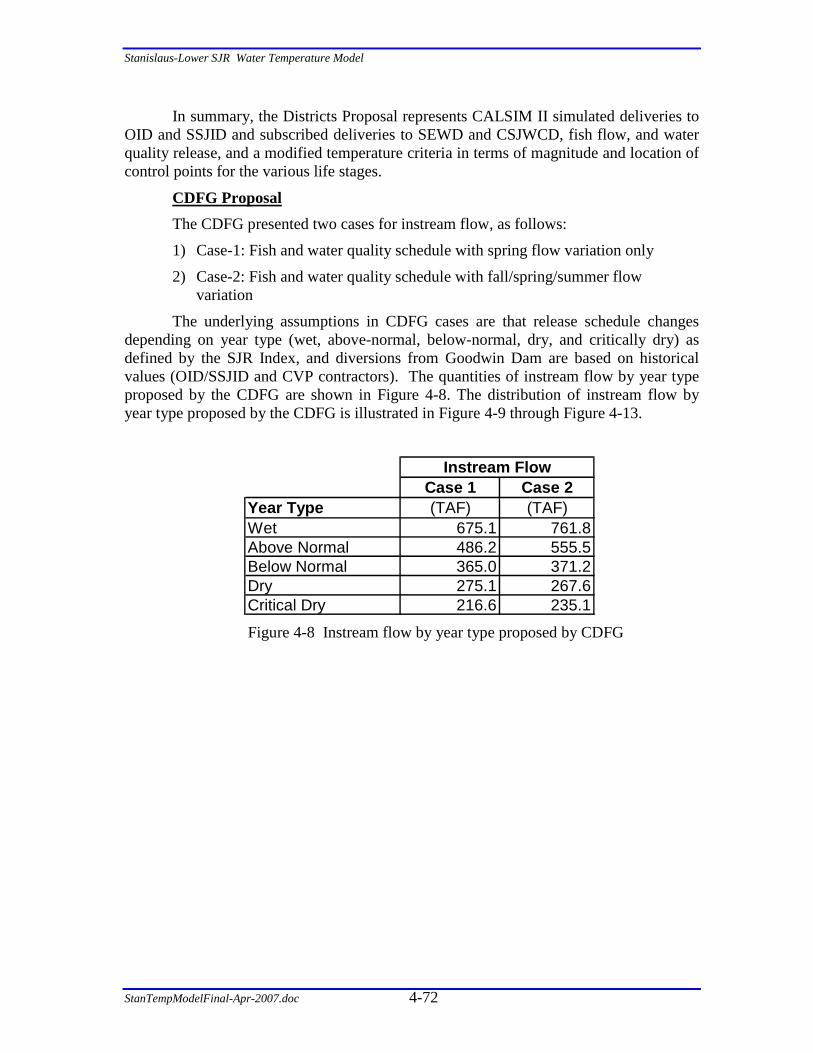
Stanislaus-Lower SJR Water Temperature Model
StanTempModelFinal-Apr-2007.doc 4-72
In summary, the Districts Proposal represents CALSIM II simulated deliveries to OID and SSJID and subscribed deliveries to SEWD and CSJWCD, fish flow, and water quality release, and a modified temperature criteria in terms of magnitude and location of control points for the various life stages.
CDFG Proposal The CDFG presented two cases for instream flow, as follows:
1) Case-1: Fish and water quality schedule with spring flow variation only
2) Case-2: Fish and water quality schedule with fall/spring/summer flow variation
The underlying assumptions in CDFG cases are that release schedule changes depending on year type (wet, above-normal, below-normal, dry, and critically dry) as defined by the SJR Index, and diversions from Goodwin Dam are based on historical values (OID/SSJID and CVP contractors). The quantities of instream flow by year type proposed by the CDFG are shown in Figure 4-8. The distribution of instream flow by year type proposed by the CDFG is illustrated in Figure 4-9 through Figure 4-13.
Case 1 Case 2Year Type (TAF) (TAF)Wet 675.1 761.8Above Normal 486.2 555.5Below Normal 365.0 371.2Dry 275.1 267.6Critical Dry 216.6 235.1
Instream Flow
Figure 4-8 Instream flow by year type proposed by CDFG
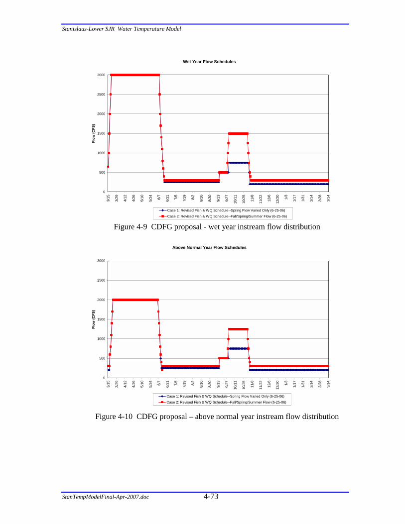
Stanislaus-Lower SJR Water Temperature Model
StanTempModelFinal-Apr-2007.doc 4-73
Figure 4-9 CDFG proposal - wet year instream flow distribution
Figure 4-10 CDFG proposal – above normal year instream flow distribution
Above Normal Year Flow Schedules
0
500
1000
1500
2000
2500
3000
3/15
3/29
4/12
4/26
5/10
5/24 6/7
6/21 7/5
7/19 8/2
8/16
8/30
9/13
9/27
10/1
1
10/2
5
11/8
11/2
2
12/6
12/2
0
1/3
1/17
1/31
2/14
2/28
3/14
Flow
(CFS
)
Case 1: Revised Fish & WQ Schedule--Spring Flow Varied Only (6-25-06)Case 2: Revised Fish & WQ Schedule--Fall/Spring/Summer Flow (6-25-06)
Wet Year Flow Schedules
0
500
1000
1500
2000
2500
3000
3/15
3/29
4/12
4/26
5/10
5/24 6/7
6/21 7/5
7/19 8/2
8/16
8/30
9/13
9/27
10/1
1
10/2
5
11/8
11/2
2
12/6
12/2
0
1/3
1/17
1/31
2/14
2/28
3/14
Flow
(CFS
)
Case 1: Revised Fish & WQ Schedule--Spring Flow Varied Only (6-25-06)Case 2: Revised Fish & WQ Schedule--Fall/Spring/Summer Flow (6-25-06)
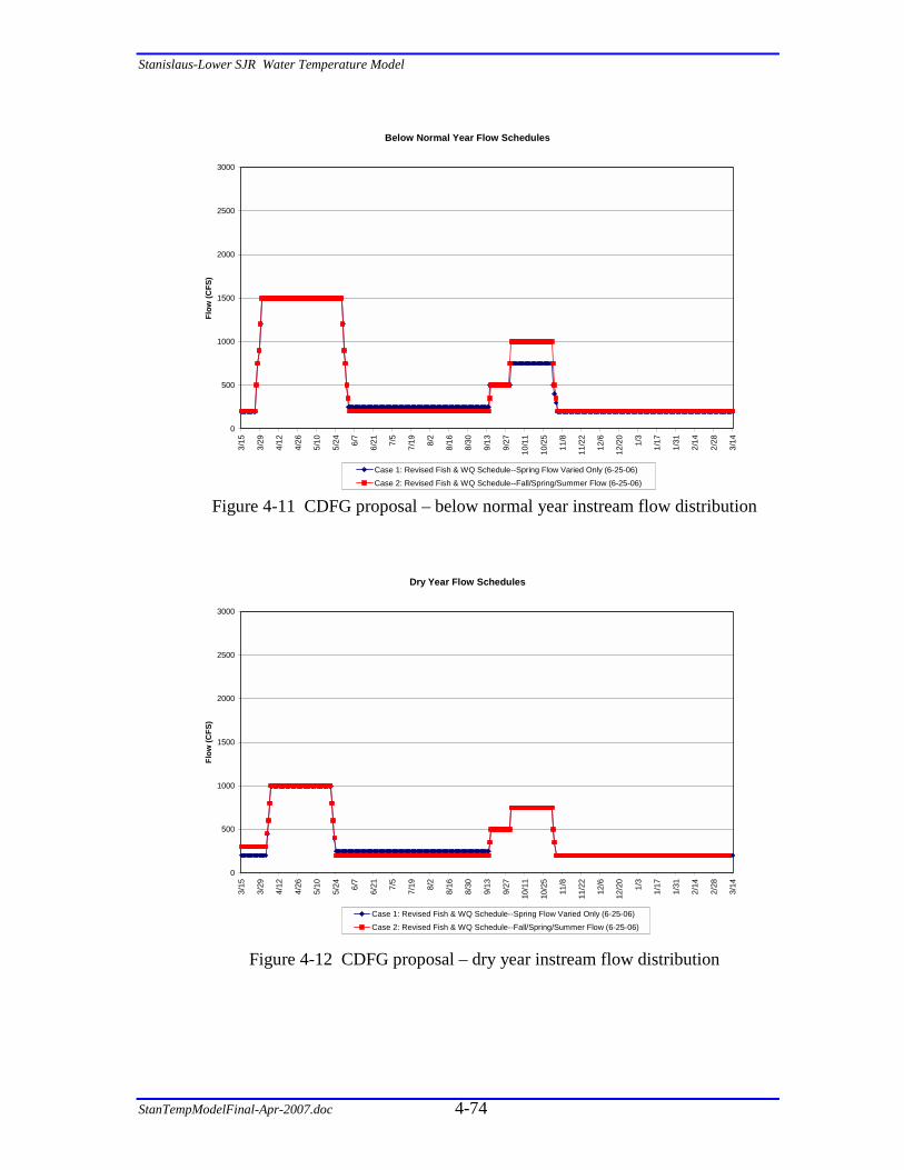
Stanislaus-Lower SJR Water Temperature Model
StanTempModelFinal-Apr-2007.doc 4-74
Figure 4-11 CDFG proposal – below normal year instream flow distribution
Figure 4-12 CDFG proposal – dry year instream flow distribution
Dry Year Flow Schedules
0
500
1000
1500
2000
2500
3000
3/15
3/29
4/12
4/26
5/10
5/24 6/7
6/21 7/5
7/19 8/2
8/16
8/30
9/13
9/27
10/1
1
10/2
5
11/8
11/2
2
12/6
12/2
0
1/3
1/17
1/31
2/14
2/28
3/14
Flow
(CFS
)
Case 1: Revised Fish & WQ Schedule--Spring Flow Varied Only (6-25-06)Case 2: Revised Fish & WQ Schedule--Fall/Spring/Summer Flow (6-25-06)
Below Normal Year Flow Schedules
0
500
1000
1500
2000
2500
3000
3/15
3/29
4/12
4/26
5/10
5/24 6/7
6/21 7/5
7/19 8/2
8/16
8/30
9/13
9/27
10/1
1
10/2
5
11/8
11/2
2
12/6
12/2
0
1/3
1/17
1/31
2/14
2/28
3/14
Flow
(CFS
)
Case 1: Revised Fish & WQ Schedule--Spring Flow Varied Only (6-25-06)Case 2: Revised Fish & WQ Schedule--Fall/Spring/Summer Flow (6-25-06)

Stanislaus-Lower SJR Water Temperature Model
StanTempModelFinal-Apr-2007.doc 4-75
Figure 4-13 CDFG proposal – critical dry year instream flow distribution
CDFG requested that the temperature analysis be conducted in two ways:
1) Using the proposed Peer Criteria,
2) Using the proposed Peer Criteria; however, moving control point locations depending on year type, as follows:
a) For the first 4 fish weeks (9/4 to 10/1): Control Point Year Type
Confluence (RM 0) Above Normal / Wet RM 15 Below Normal RM 30 Critical / Dry
b) For the next 6 fish weeks (10/2 to 11/12): Control Point Year Type
RM 34 Above Normal / Wet RM 39 Below Normal RM 44 Critical / Dry
The resulting modified temperature criteria proposed by CDFG are illustrated in Figure 4-14 through Figure 4-16.
Critical Year Flow Schedules
0
500
1000
1500
2000
2500
3000
3/15
3/29
4/12
4/26
5/10
5/24 6/7
6/21 7/5
7/19 8/2
8/16
8/30
9/13
9/27
10/1
1
10/2
5
11/8
11/2
2
12/6
12/2
0
1/3
1/17
1/31
2/14
2/28
3/14
Flow
(CFS
)
Case 1: Revised Fish & WQ Schedule--Spring Flow Varied Only (6-25-06)Case 2: Revised Fish & WQ Schedule--Fall/Spring/Summer Flow (6-25-06)

Stanislaus-Lower SJR Water Temperature Model
StanTempModelFinal-Apr-2007.doc 4-76
CDFG Year Type: Wet / Above Normal
Calendar Date
Fish Week Location Lifestage
WEEKLY Criteria
(A) (B) (C) (E)7-Day AOM
(deg F)9/4 1 Confluence Adult 64.0
9/11 2 Confluence Adult 64.09/18 3 Confluence Adult 64.09/25 4 Confluence Adult 64.010/2 5 RM 34 (~McHenry Br.) Egg Incubation 55.010/9 6 RM 34 Egg Incubation 55.0
10/16 7 RM 34 Egg Incubation 55.010/23 8 RM 34 Egg Incubation 55.010/30 9 RM 34 Egg Incubation 55.0
11/6 10 RM 34 Egg Incubation 55.011/13 11 Riverbank Egg Incubation 55.011/20 12 Riverbank Egg Incubation 55.011/27 13 Riverbank Egg Incubation 55.0
12/4 14 Riverbank Egg Incubation 55.012/11 15 Riverbank Egg Incubation 55.012/18 16 Riverbank Egg Incubation 55.012/25 17 Riverbank Egg Incubation 55.0
1/1 18 Riverbank Juvenile Rearing 61.01/8 19 Riverbank Juvenile Rearing 61.0
1/15 20 Riverbank Juvenile Rearing 61.01/22 21 Riverbank Juvenile Rearing 61.01/29 22 Riverbank Juvenile Rearing 61.02/5 23 Riverbank Juvenile Rearing 61.0
2/12 24 Riverbank Juvenile Rearing 61.02/19 25 Riverbank Juvenile Rearing 61.02/26 26 Riverbank Juvenile Rearing 61.03/5 27 Riverbank Juvenile Rearing 61.0
3/12 28 Riverbank Juvenile Rearing 61.03/19 29 Riverbank Juvenile Rearing 61.03/26 30 Riverbank Juvenile Rearing 61.04/2 31 Riverbank Juvenile Rearing 61.04/9 32 Riverbank Juvenile Rearing 61.0
4/16 33 Confluence smoltification 57.04/23 34 Confluence smoltification 57.04/30 35 Confluence smoltification 57.05/7 36 Confluence smoltification 57.0
5/14 37 Confluence smoltification 57.05/21 38 Confluence smoltification 57.05/28 39 Confluence smoltification 57.06/4 40 Orange Blossom Juvenile Reaering 64.0
6/11 41 Orange Blossom Juvenile Reaering 64.06/18 42 Orange Blossom Juvenile Reaering 64.06/25 43 Orange Blossom Juvenile Reaering 64.07/2 44 Orange Blossom Juvenile Reaering 64.07/9 45 Orange Blossom Juvenile Reaering 64.0
7/16 46 Orange Blossom Juvenile Reaering 64.07/23 47 Orange Blossom Juvenile Reaering 64.07/30 48 Orange Blossom Juvenile Reaering 64.08/6 49 Orange Blossom Juvenile Reaering 64.0
8/13 50 Orange Blossom Juvenile Reaering 64.08/20 51 Orange Blossom Juvenile Reaering 64.08/27 52 Orange Blossom Juvenile Reaering 64.0
Figure 4-14 Temperature criteria for wet and above normal years proposed by CDFG

Stanislaus-Lower SJR Water Temperature Model
StanTempModelFinal-Apr-2007.doc 4-77
CDFG Year Type: Below Normal
Calendar Date
Fish Week Location Lifestage
WEEKLY Criteria
(A) (B) (C) (E)7-Day AOM
(deg F)9/4 1 RM 15 (~Ripon) Adult 64.0
9/11 2 RM 15 Adult 64.09/18 3 RM 15 Adult 64.09/25 4 RM 15 Adult 64.010/2 5 RM 39 (~Riverbank) Egg Incubation 55.010/9 6 RM 39 Egg Incubation 55.0
10/16 7 RM 39 Egg Incubation 55.010/23 8 RM 39 Egg Incubation 55.010/30 9 RM 39 Egg Incubation 55.0
11/6 10 RM 39 Egg Incubation 55.011/13 11 Riverbank Egg Incubation 55.011/20 12 Riverbank Egg Incubation 55.011/27 13 Riverbank Egg Incubation 55.0
12/4 14 Riverbank Egg Incubation 55.012/11 15 Riverbank Egg Incubation 55.012/18 16 Riverbank Egg Incubation 55.012/25 17 Riverbank Egg Incubation 55.0
1/1 18 Riverbank Juvenile Rearing 61.01/8 19 Riverbank Juvenile Rearing 61.0
1/15 20 Riverbank Juvenile Rearing 61.01/22 21 Riverbank Juvenile Rearing 61.01/29 22 Riverbank Juvenile Rearing 61.02/5 23 Riverbank Juvenile Rearing 61.0
2/12 24 Riverbank Juvenile Rearing 61.02/19 25 Riverbank Juvenile Rearing 61.02/26 26 Riverbank Juvenile Rearing 61.03/5 27 Riverbank Juvenile Rearing 61.0
3/12 28 Riverbank Juvenile Rearing 61.03/19 29 Riverbank Juvenile Rearing 61.03/26 30 Riverbank Juvenile Rearing 61.04/2 31 Riverbank Juvenile Rearing 61.04/9 32 Riverbank Juvenile Rearing 61.0
4/16 33 Confluence smoltification 57.04/23 34 Confluence smoltification 57.04/30 35 Confluence smoltification 57.05/7 36 Confluence smoltification 57.0
5/14 37 Confluence smoltification 57.05/21 38 Confluence smoltification 57.05/28 39 Confluence smoltification 57.06/4 40 Orange Blossom Juvenile Reaering 64.0
6/11 41 Orange Blossom Juvenile Reaering 64.06/18 42 Orange Blossom Juvenile Reaering 64.06/25 43 Orange Blossom Juvenile Reaering 64.07/2 44 Orange Blossom Juvenile Reaering 64.07/9 45 Orange Blossom Juvenile Reaering 64.0
7/16 46 Orange Blossom Juvenile Reaering 64.07/23 47 Orange Blossom Juvenile Reaering 64.07/30 48 Orange Blossom Juvenile Reaering 64.08/6 49 Orange Blossom Juvenile Reaering 64.0
8/13 50 Orange Blossom Juvenile Reaering 64.08/20 51 Orange Blossom Juvenile Reaering 64.08/27 52 Orange Blossom Juvenile Reaering 64.0
Figure 4-15 Temperature criteria for below normal years proposed by CDFG
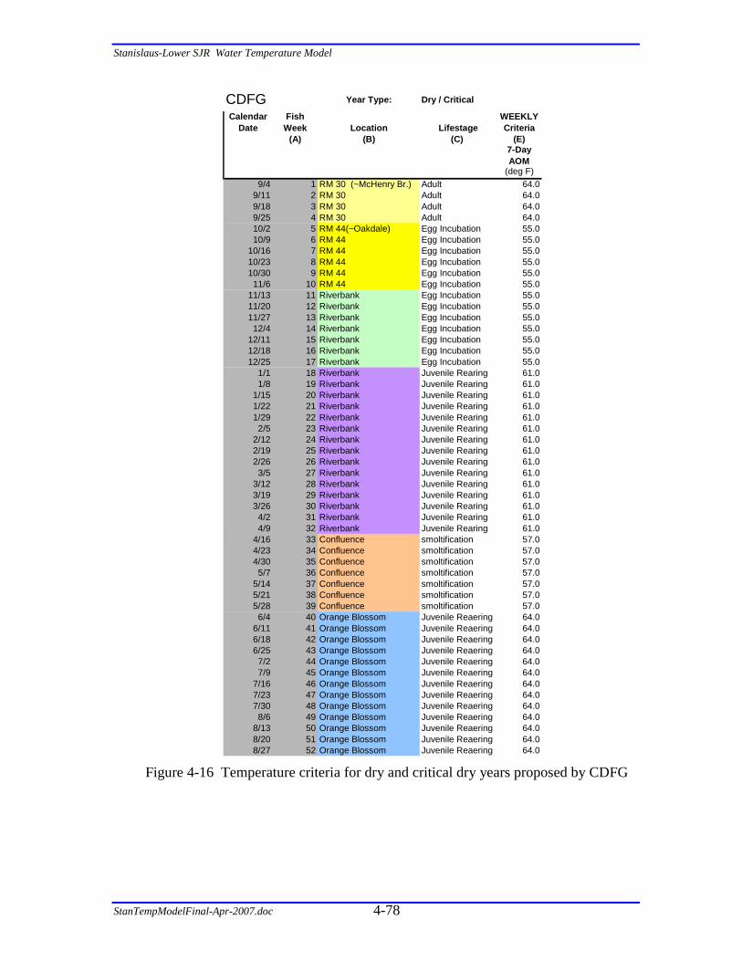
Stanislaus-Lower SJR Water Temperature Model
StanTempModelFinal-Apr-2007.doc 4-78
CDFG Year Type: Dry / Critical
Calendar Date
Fish Week Location Lifestage
WEEKLY Criteria
(A) (B) (C) (E)7-Day AOM
(deg F)9/4 1 RM 30 (~McHenry Br.) Adult 64.0
9/11 2 RM 30 Adult 64.09/18 3 RM 30 Adult 64.09/25 4 RM 30 Adult 64.010/2 5 RM 44(~Oakdale) Egg Incubation 55.010/9 6 RM 44 Egg Incubation 55.0
10/16 7 RM 44 Egg Incubation 55.010/23 8 RM 44 Egg Incubation 55.010/30 9 RM 44 Egg Incubation 55.011/6 10 RM 44 Egg Incubation 55.0
11/13 11 Riverbank Egg Incubation 55.011/20 12 Riverbank Egg Incubation 55.011/27 13 Riverbank Egg Incubation 55.012/4 14 Riverbank Egg Incubation 55.0
12/11 15 Riverbank Egg Incubation 55.012/18 16 Riverbank Egg Incubation 55.012/25 17 Riverbank Egg Incubation 55.0
1/1 18 Riverbank Juvenile Rearing 61.01/8 19 Riverbank Juvenile Rearing 61.0
1/15 20 Riverbank Juvenile Rearing 61.01/22 21 Riverbank Juvenile Rearing 61.01/29 22 Riverbank Juvenile Rearing 61.02/5 23 Riverbank Juvenile Rearing 61.0
2/12 24 Riverbank Juvenile Rearing 61.02/19 25 Riverbank Juvenile Rearing 61.02/26 26 Riverbank Juvenile Rearing 61.03/5 27 Riverbank Juvenile Rearing 61.0
3/12 28 Riverbank Juvenile Rearing 61.03/19 29 Riverbank Juvenile Rearing 61.03/26 30 Riverbank Juvenile Rearing 61.04/2 31 Riverbank Juvenile Rearing 61.04/9 32 Riverbank Juvenile Rearing 61.0
4/16 33 Confluence smoltification 57.04/23 34 Confluence smoltification 57.04/30 35 Confluence smoltification 57.05/7 36 Confluence smoltification 57.0
5/14 37 Confluence smoltification 57.05/21 38 Confluence smoltification 57.05/28 39 Confluence smoltification 57.06/4 40 Orange Blossom Juvenile Reaering 64.0
6/11 41 Orange Blossom Juvenile Reaering 64.06/18 42 Orange Blossom Juvenile Reaering 64.06/25 43 Orange Blossom Juvenile Reaering 64.07/2 44 Orange Blossom Juvenile Reaering 64.07/9 45 Orange Blossom Juvenile Reaering 64.0
7/16 46 Orange Blossom Juvenile Reaering 64.07/23 47 Orange Blossom Juvenile Reaering 64.07/30 48 Orange Blossom Juvenile Reaering 64.08/6 49 Orange Blossom Juvenile Reaering 64.0
8/13 50 Orange Blossom Juvenile Reaering 64.08/20 51 Orange Blossom Juvenile Reaering 64.08/27 52 Orange Blossom Juvenile Reaering 64.0
Figure 4-16 Temperature criteria for dry and critical dry years proposed by CDFG

Stanislaus-Lower SJR Water Temperature Model
StanTempModelFinal-Apr-2007.doc 4-79
Assumptions: The following assumptions were used in analyzing the Districts and CDFG cases:
• The simulation period was 1982-2004.
• In all proposed cases, New Melones power plant was bypassed during the period September 15 to November 13 if reservoir levels falls below El. 900 feet on Sept. 15 (see Alternative D in Section 4.3.2).
• All results were compared with respect to historical operations.
• Energy price (for loss of generation due to New Melones power plant bypass) was based on current energy pricing offered by PG&E to all Qualifying Facilities (QF) projects of $64.50 per megawatt-hour for a 5-year fixed term.
• Under the Districts proposed operation, New Melones was completely dry by June 15, 1992. The model continued to run, but allocated the total New Melones outflow (outflow = inflow) to the diversion at Goodwin leaving the release to the river below Goodwin Dam as zero. The following procedure was used to reallocate diversion flows to the Stanislaus River once New Melones volume reached 5,000 AF:
i. Decrease diversions so that the Goodwin release to the river equaled the minimum required flow.
ii. If New Melones outflow was less than the minimum Goodwin flow to the river, diversions were set to zero and all available flow was released to the river.
iii. Tulloch was not re-operated to meet diversion or instream flows.
Results The results are presented in several ways:
1) A chart showing New Melones Storage for all cases.
2) A chart showing New Melones Elevation for all cases.
3) A table showing minimum New Melones storage in the critical year and temperature violations with respect to the Historical Case based on the Peer Criteria, Districts Criteria, and CDFG Criteria.
4) A table showing the foregone power resulting from bypassing New Melones power plant between September 15 and November 13 during years when New Melones elevation was below 900 feet on September 15.
5) Charts showing temperature violations for each case.
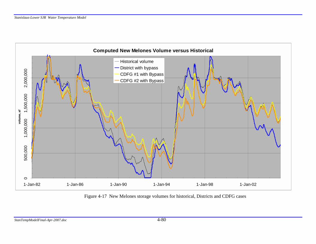
Stanislaus-Lower SJR Water Temperature Model
StanTempModelFinal-Apr-2007.doc
4-80
Figure 4-17 New Melones storage volumes for historical, Districts and CDFG cases
Computed New Melones Volume versus Historical
050
0,00
01,
000,
000
1,50
0,00
02,
000,
000
1-Jan-82 1-Jan-86 1-Jan-90 1-Jan-94 1-Jan-98 1-Jan-02
volu
me,
af
Historical volumeDistrict with bypassCDFG #1 with BypassCDFG #2 with Bypass

Stanislaus-Lower SJR Water Temperature Model
StanTempModelFinal-Apr-2007.doc 4-81
Figure 4-18 New Melones water surface elevation for historical, Districts and CDFG cases
Computed New Melones Elevation versus HistoricalBypass Trigger = El. 900, Bypass Period = Sept. 15 to Nov. 13
600
700
800
900
1,000
1,100
1-Jan-82 1-Jan-86 1-Jan-90 1-Jan-94 1-Jan-98 1-Jan-02
elev
atio
n, ft
Historical elevationDistrict with bypassCDFG #1 with BypassCDFG #2 with BypassBypass Trigger
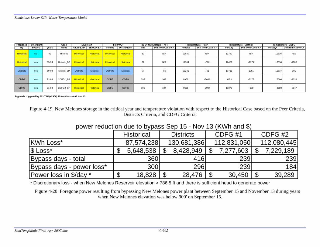
Stanislaus-Lower SJR Water Temperature Model
StanTempModelFinal-Apr-2007.doc 4-82
Figure 4-19 New Melones storage in the critical year and temperature violation with respect to the Historical Case based on the Peer Criteria, Districts Criteria, and CDFG Criteria.
Figure 4-20 Foregone power resulting from bypassing New Melones power plant between September 15 and November 13 during years
when New Melones elevation was below 900' on September 15.
Historical Districts CDFG #1 CDFG #2KWh Loss* 87,574,238 130,681,386 112,831,050 112,080,445$ Loss* 5,648,538$ 8,428,949$ 7,277,603$ 7,229,189$ Bypass days - total 360 416 239 239Bypass days - power loss* 300 296 239 184Power loss in $/day * 18,828$ 28,476$ 30,450$ 39,289$ * Discretionary loss - when New Melones Reservoir elevation > 786.5 ft and there is sufficient head to generate power
power reduction due to bypass Sep 15 - Nov 13 (KWh and $)
Proposed Powerplant CaseBy Bypass years Name OID/SSJID SEWD/CSJ Volume Distribution Min. Diff from Case 0-A Penalty Diff from Case 0-A Penalty Diff from Case 0-A Penalty* Diff from Case 0-A
Historical No 92 Historic Historical Historical Historical Historical 87 N/A 12540 N/A 11750 N/A 11536 N/A
Historical Yes 89-94 Historic_BP Historical Historical Historical Historical 87 N/A 11764 -776 10476 -1274 10536 -1000
Districts Yes 89-94 District_BP Districts Districts Districts Districts 2 -85 13241 701 13711 1961 11837 301
CDFG Yes 91-94 CDFG1_BP Historical Historical CDFG CDFG 395 308 8906 -3634 9473 -2277 7500 -4036
CDFG Yes 91-94 CDFG2_BP Historical Historical CDFG CDFG 191 104 9636 -2904 11070 -680 8589 -2947
Bypassis triggered by 723 TAF (el 900) 15 sept lasts until Nov 13
Diversion Fish/WQ Temperature - Peer Temperature - District83-04 NM Storage (TAF) Temperature - CDFG

Stanislaus-Lower SJR Water Temperature Model
StanTempModelFinal-Apr-2007.doc 4.83
Figure 4-21 Evaluation of cases using Peer Criteria
HistoricCDFG1_BP-Peer
HistoricCDFG2_BP-Peer
HistoricDist_BP-Peer
HistoricHistoric_BP-Peer
0
200
400
600
8001000
1200
1400
1600
1800
2000
1/1 4/1 7/1 9/29 12/29W
eekl
y C
riter
ia P
enal
ty
Historic
(Scenario)Historic:Scenario:Change:
125408906-3634
Historic vs Scenario
0
200
400
600
8001000
1200
1400
1600
1800
2000
1/1 4/1 7/1 9/29 12/29
Wee
kly
Crit
eria
Pen
alty
Historic
(Scenario)Historic:Scenario:Change:
125409636-2904
Historic vs Scenario
0200
400
600
800
1000
1200
1400
1600
1800
2000
1/1 4/1 7/1 9/29 12/29
Wee
kly
Crit
eria
Pen
alty
Historic
(Scenario)Historic:Scenario:Change:
1254013241701
Historic vs Scenario
0
200
400
600
8001000
1200
1400
1600
1800
2000
1/1 4/1 7/1 9/29 12/29
Wee
kly
Crit
eria
Pen
alty
Historic
(Scenario)Historic:Scenario:Change:
1254011764-776
Historic vs Scenario
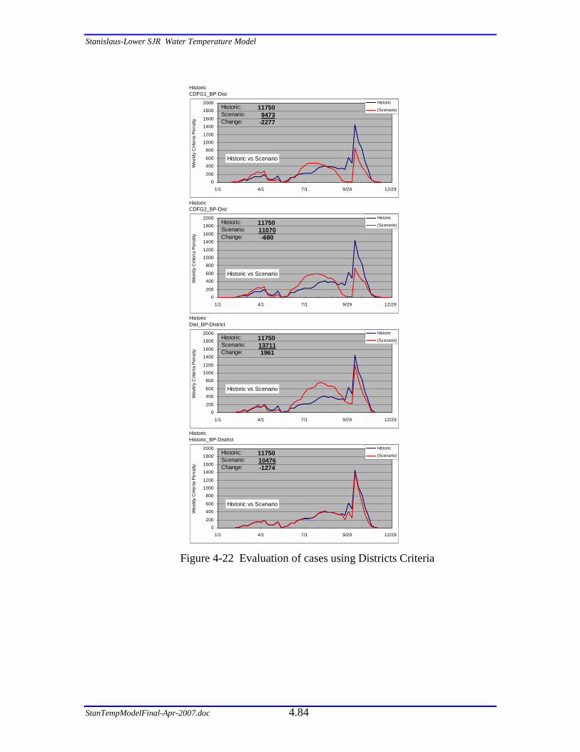
Stanislaus-Lower SJR Water Temperature Model
StanTempModelFinal-Apr-2007.doc 4.84
Figure 4-22 Evaluation of cases using Districts Criteria
HistoricCDFG1_BP-Dist
HistoricCDFG2_BP-Dist
HistoricDist_BP-District
HistoricHistoric_BP-District
0
200
400
600
800
1000
1200
1400
1600
1800
2000
1/1 4/1 7/1 9/29 12/29W
eekl
y C
riter
ia P
enal
ty
Historic
(Scenario)Historic:Scenario:Change:
117509473
-2277
Historic vs Scenario
0
200
400
600
800
1000
1200
1400
1600
1800
2000
1/1 4/1 7/1 9/29 12/29
Wee
kly
Crit
eria
Pen
alty
Historic
(Scenario)Historic:Scenario:Change:
1175011070-680
Historic vs Scenario
0
200
400
600
800
1000
1200
1400
1600
1800
2000
1/1 4/1 7/1 9/29 12/29
Wee
kly
Crit
eria
Pen
alty
Historic
(Scenario)Historic:Scenario:Change:
11750137111961
Historic vs Scenario
0
200
400
600
800
1000
1200
1400
1600
1800
2000
1/1 4/1 7/1 9/29 12/29
Wee
kly
Crit
eria
Pen
alty
Historic
(Scenario)Historic:Scenario:Change:
1175010476-1274
Historic vs Scenario
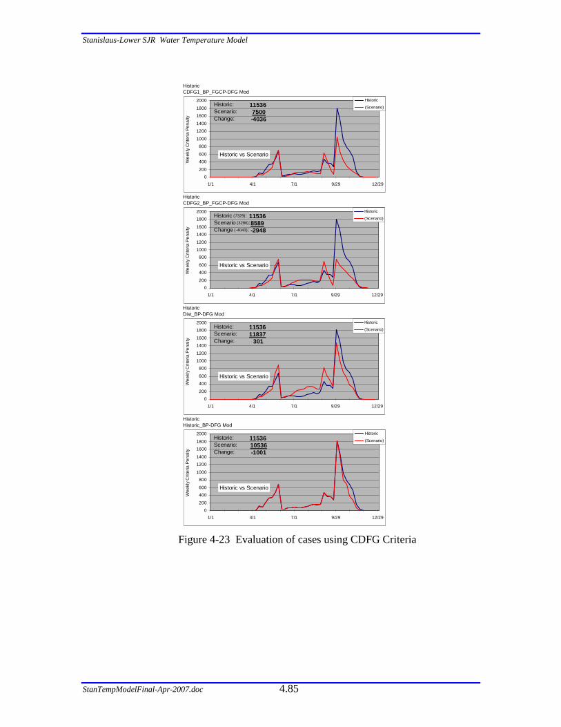
Stanislaus-Lower SJR Water Temperature Model
StanTempModelFinal-Apr-2007.doc 4.85
Figure 4-23 Evaluation of cases using CDFG Criteria
HistoricCDFG1_BP_FGCP-DFG Mod
HistoricCDFG2_BP_FGCP-DFG Mod
HistoricDist_BP-DFG Mod
HistoricHistoric_BP-DFG Mod
0
200
400
600
800
1000
1200
1400
1600
1800
2000
1/1 4/1 7/1 9/29 12/29
Wee
kly
Crit
eria
Pen
alty
Historic
(Scenario)Historic:Scenario:Change:
1153610536-1001
Historic vs Scenario
0
200
400
600
800
1000
1200
1400
1600
1800
2000
1/1 4/1 7/1 9/29 12/29
Wee
kly
Crit
eria
Pen
alty
Historic
(Scenario)Historic:Scenario:Change:
1153611837
301
Historic vs Scenario
0
200
400
600
800
1000
1200
1400
1600
1800
2000
1/1 4/1 7/1 9/29 12/29W
eekl
y C
riter
ia P
enal
ty
Historic
(Scenario)Historic:Scenario:Change:
115367500-4036
Historic vs Scenario
0200
400
600
800
1000
1200
1400
1600
1800
2000
1/1 4/1 7/1 9/29 12/29
Wee
kly
Crit
eria
Pen
alty
Historic
(Scenario)Historic (7329):Scenario (3286):Change (-4043):
115368589-2948
Historic vs Scenario
Stanislaus-Lower SJR Water Temperature Model
StanTempModelFinal-Apr-2007.doc 4.86
Findings The alternative operations cases proposed by the Districts and CDFG were
analyzed using the flow and temperature model. The results were subsequently evaluated based on the Peer Criteria, Districts’ Criteria, and CDFG Criteria.
The main difference between the Districts’ Case and CDFG Cases was the assumption regarding diversions. While CDFG uses historical diversion from Goodwin, the District Case providedd assumed deliveries based on future demands by the irrigation districts subject to the Districts’ proposed curtailments based on New Melones Index.
From the temperature response point of view, the results differ among the alternatives, but generally late spring and early fall present the most challenging periods for anadromous fish in the river. In the spring period, the Districts’ case and criteria provided the best performance. During the summer period, the CDFG1 Case, with either the Peer or CDFG Criteria, provided the best performance. In the fall, both the CDFG1 and CDFG2 Cases provided improvement over historic conditions. The District Case showed reduced penalty, but this reduction varied considerably among the selected criteria, at times accruing more penalty than the historic condition.
In conclusion: these simulations provide potentially useful insight into several facets of flow and temperature management in the Stanislaus River system, including:
• For approximately 8 months of the year, there are low penalties and generally little difference among many of the scenarios and criteria.
• There appear to be clear bottle necks in the river in the spring (smoltification) and fall (early adult immigration and egg incubation).
• The system may be operated in various manners resulting in different benefits or dis-benefits.
• The model and peer review criteria spreadsheet can readily identify the impacts of various water management strategies and sensitivity of selected thermal criteria

Stanislaus-Lower SJR Water Temperature Model
StanTempModelFinal-Apr-2007.doc 4.87
4.3.2 Other Operational and Physical Changes
In addition to the operations proposed by the Districts and CDFG, other operational and physical changes were developed through discussions with the stakeholders or initiated by the project team. These concepts are stand-alone options and, if feasible, could be implemented in conjunction with the Water Management Plans proposed by the Districts and CDFG.
To assess potential impacts of operational changes, a base case and seven alternatives were simulated for the 1988 through 1997 period, a time of extended drought and reservoir recovery:
A. Re-operation using Tulloch Rule Curve (base case) B. Tulloch re-operation (September drawdown and filling C. Old Melones Dam removal D. New Melones power bypass with and without Old Melones Dam
(various dates) E. Goodwin Dam Retrofit (lower level outlet) F. New Melones selective withdrawal (with and without Old Melones
Dam) G. New Melones power outlet extension (without old dam) H. Old Melones lowered 55 feet (partial removal)
Results were output to DSS at six-hour intervals at the following locations:
o New Melones Dam (RM 69)
o Tulloch Dam (RM 60)
o Goodwin Dam (RM 58)
o Stanislaus at Knights Ferry (RM 54)
o Stanislaus at Orange Blossom Br. (RM 46)
o Stanislaus at Oakdale Recreation Area (RM 40)
o Stanislaus at Riverbank (RM 31)
o Stanislaus at Ripon (RM 15)
o Stanislaus at San Joaquin Confluence (RM 0)
o San Joaquin at Vernalis (RM 72 on the SJR)
The data storage system (DSS) file structure consists of several “parts” that describe various aspects of the data set. This structure provided a convenient method to store simulation results in DSS for dissemination, review, and assessment by stakeholders. For example, the F-parts in the DSS file indicate the alternative operation and/or physical change. Table 4-2 lists the F-parts with descriptions of the alternatives. There are more than seven alternatives due to permutations of a particular alternative.

Stanislaus-Lower SJR Water Temperature Model
StanTempModelFinal-Apr-2007.doc 4.88
Table 4-2 DSS F parts and descriptions for 1988–1997 simulation period results.
F part Description historical Historical flows and operation (base case) Tulloch_reopp Tulloch re-operation (September drawdown - 30 TAF max) Select New Melones selective withdrawal (725’ - 875’) Goodwin_retro Goodwin Dam retrofit Sep_BP New Melones power plant bypass on September 15 Aug_BP New Melones power plant bypass on August 15 May_Aug_BP New Melones power plant bypass in May 2 and August 15 May_Sep_BP New Melones power plant bypass in May 2 and September 15 no_dam Old Melones Dam removed (no bypass or selective withdrawal) ND_Jul_BP Old Melones Dam removed with July 15 bypass ND_Aug_BP Old Melones Dam removed with August 15 bypass ND_Sep_BP Old Melones Dam removed with September 15 bypass ND_select Old Melones Dam removed with selective withdrawal (675’ – 875’) ND_May_Sep_BP Old Melones Dam removed with May 2 and September 15 bypass ND_May_Aug_BP Old Melones Dam removed with May 2 and August 15 bypass D2_May_Aug_BP Old Melones Dam lowered 55ft with May 2 and August 15 bypass D2_Pow_100ft Old Melones Dam lowered 55ft with 100 ft lower power D2_Aug_100_BP Old Melones Dam lowered 55ft with 100 ft lower power & August bypass
Results for the individual alternatives are discussed in detail below. Graphical results for each case represent a one year period that represents average weekly maximums over the entire 6-year evaluation period from April 1989 through April 1995 (see discussion under base case, below).
A. Re-operation using Tulloch Rule Curve (base case) The base case used for comparison with operational and physical changes was a
modified-historical simulation. The base case used historical New Melones reservoir inflows with minor modification to outflows. New Melones reservoir outflows were modified to ensure Tulloch reservoir volume effectively tracked the storage rule curve, eliminating any impacts from atypical operations such as the 1991 Tulloch drawdown. Note, the base case is also referred to as “historical” in the plots.

Stanislaus-Lower SJR Water Temperature Model
StanTempModelFinal-Apr-2007.doc 4.89
Average weekly maximum and maximum weekly maximum temperatures at Goodwin Dam for historical flows over the 6-year evaluation period are shown in Figure 4-24. The inset plot includes 6-hour temperatures at Goodwin Dam for 1992. Elevated Goodwin temperatures result for discharge of near surface New Melones water prior to discontinued power plant operation in June (due to power intake submergence requirements) and surfacing of the Old dam in the fall. The impact of the 1992 results is clearly seen in the plot of weekly maximum temperatures. Because there are no flow changes in the alternatives, the June shut-off date and associated maximum temperature is the same except for power bypass or selective withdrawal options and the September dam surfacing and associated maximum temperature is the same for all alternatives that do not include dam removal. Therefore, results are presented as average weekly maximum temperatures for all subsequent plots so that conditions among all alternatives can be readily compared.
B. Tulloch re-operation (September drawdown and filling) In 1991 Tulloch Reservoir was drawn down and refilled with cold water from the
New Melones low-level outlet (i.e., bypassing the power plant). The Tulloch re-operation alternative was performed to determine how much of the thermal impact observed during this 1991 event was the result of drawdown and how much was the result of power plant bypass.
The Tulloch re-operation alternative involved modification of New Melones reservoir releases beginning on September 15 of each year to drawdown Tulloch Reservoir up to 30 TAF, or until September 30, whichever occurred first. On September 30, inflows were increased by an amount equivalent to the flow reduction for drawdown, to refill the reservoir by October 13. An example of this operation is shown in Figure 4-25 for 1993.
There was no impact of this operation on flow at Goodwin Dam and very little change in temperature was observed at Goodwin Dam in simulation results. Figure 4-26 shows the average temperature impact at Goodwin Dam over the evaluation period. Base case versus Tulloch drawdown temperatures showed an increase in temperature of approximately 3° F during the drawdown period. Beginning in October, there was a temperature benefit of approximately 1° F that lasted through the month.
C. Old Melones Dam removal Removal of Old Melones Dam was simulated to investigate the impacts of
potentially greater access to the lower portions of the cold water pool. No other operational changes were assessed in this alternative. A plot of computed 7-day average maximum temperatures at Goodwin Dam for the base case and Old Melones Dam removal alternative is provided in Figure 4-27.
There was almost no impact on temperature with the removal of the dam (assuming no other operational changes). This is largely due to power plant operations: power plant bypass must commence when water surface elevations fall below 780 feet to avoid air entrainment, and thus if the dam is in place there is still cold water flowing over it. The differences in average temperatures between the base case and old dam removal alternative were almost solely due to 1992 operation when the power plant was bypassed

Stanislaus-Lower SJR Water Temperature Model
StanTempModelFinal-Apr-2007.doc 4.90
due to elevation constraints. This is illustrated in the inset plot in Figure 4-27, which shows 6-hour temperature results for 1992 for the base case and the old dam removal alternative. In this case, having the dam in place was actually a benefit. With the old dam removed, the low-level outlet depleted the entire cold water pool and by September, only warmer water remained. With the old dam in place, cold water was stored behind the dam resulting in lower temperatures during September and October. By this time, the water surface elevation dropped below the old dam and flow was through the low-level outlet in the old dam accessing the cold water stored behind it.
D. New Melones power bypass with and without Old Melones Dam (various dates)
Uner the current configuration, the New Melones power plant intake is located at an elevation of 760 feet (invert elevation) and the low-level outlet elevation is located at 543 feet. Because the low level outlet accesses deeper water, bypass of the New Melones power plant flows to the low-level outlet could serve as an alternative to constructing a temperature control device in New Melones Reservoir.
For the New Melones power bypass alternative, New Melones Power Plant flows were bypassed to the low-level outlet for years when the New Melones storage elevation is greater than 900’ on September 15. Three operations strategies for the power plant bypass were examined, namely bypassing during the periods:
• September 15 – November 12,
• August 15 – November 12, or
• May 2 – May 23 and August 15 – November 12 Computed 7-day average maximum temperatures for the base case and three New
Melones power bypass schedules with the Old Melones Dam are plotted in Figure 4-28.
For the September 15 – November 12 bypass operation, Goodwin Dam release temperatures in October were reduced by approximately 7° F with total forgone power production of 86,400 MWH or $5,620,000 (based on $.065/KWH).
For the August 15 – November 12 bypass operation, the temperatures of the warmest releases were reduced, but some of the beneficial effect seen with the September bypass date was reduced in September and October. October temperatures were reduced by approximately 4° F with total forgone power production of 227,400 MWH or $14,780,000. The smaller reduction with the August 15 bypass date demonstrated the limited volume of cold water available with the old dam in place.
The May 2 – May 23 bypass to provided a pulse flow in the spring (i.e., adding 21 day bypass period in May) had little impact on October temperatures and small thermal benefits in May.
Additional simulations were completed with Old Melones Dam removed – effectively providing access to more cold water. An additional simulation with a bypass period of July 15 – November 12 was simulated as a sensitivity test to determine how much cold water is potentially available. Computed 7-day average maximum temperatures for the base case, along with New Melones power bypass schedules for July
Stanislaus-Lower SJR Water Temperature Model
StanTempModelFinal-Apr-2007.doc 4.91
15 – November 12, August 15 – November 12, and September 15 – November 12 with the Old Melones Dam removed are plotted in Figure 4-29.
For bypass operations commencing on September 15, October temperatures were reduced by approximately 8° F. Starting such operations in September had no impact on the warmest release temperatures that occur in late August.
For bypass operations commencing on August 15, temperatures of the warmest releases in August were decreased; however, October temperatures were not reduced to the same extent as bypass operation starting on September 15. October temperatures were reduced by approximately 7° F, approximately 1° F difference from the September 15 bypass operation. Nonetheless, this was an improvement of 3° F over results with the old dam in place. Thus, with removal of the old dam, it was possible to begin power bypass approximately one month earlier than with the old dam in place, and achieve similar benefits in October and additional benefits in August and September.
For bypass operations commencing on July15, October temperatures were reduced by approximately 3° F. The smaller reduction demonstrated the cool water pool remains limited even with the old dam removed.
A plot of base case and the August 15 – November 12 power bypass alternative with and without Old Melones Dam is shown in Figure 4-33. With the dam removed, temperatures during late August through October were approximately 2.5° F lower than with the old dam in place.
E. Goodwin Dam Retrofit (lower level outlet) The idea of modifying the operation of Goodwin Dam to enable discharging
colder water from Goodwin pool to the Stanislaus River was discussed with the Stanislaus stakeholders on several occasions over the years.
Measurements of water temperature in Goodwin pool on hot summer days, especially when instream release from the dam is low (below 300 cfs), identified stratification in the Goodwin pool. Under the present operation of the dam, the top layer of warm water in Goodwin pool is “skimmed off” and released over the crest of Goodwin Dam for the instream flow while the irrigation districts receive colder water through the irrigation canals (north and south).
The concept behind the proposed Goodwin Retrofit is to construct a low level outlet that will facilitate the transfer of cool water from Goodwin pool downstream into the Stanislaus River in lieu of discharging warm water over Goodwin Dam. The low level intake elevation would be at a sufficient depth in order to tap the lower temperature water, and release it downstream for the enhancement of the fish habitat.
The most cost effective configuration for the low level outlet appears to be at the right abutment inside the confines of the joint head-works irrigation canal (SSJID/OID joint canal).
The intake of the irrigation canal is controlled by three 72-inch by 120-inch slide gates also referred to as the upper gates. Downstream of the upper gates there are three identical gates, referred to as the lower gates. The lower gates are normally left in the
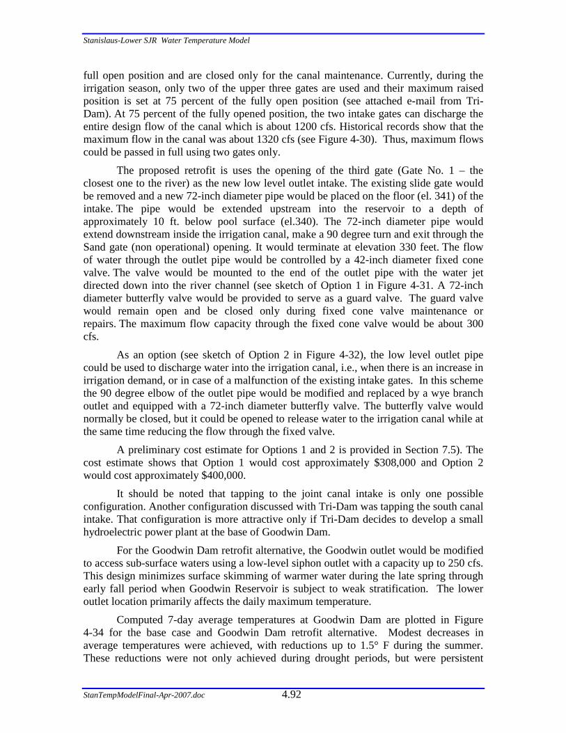
Stanislaus-Lower SJR Water Temperature Model
StanTempModelFinal-Apr-2007.doc 4.92
full open position and are closed only for the canal maintenance. Currently, during the irrigation season, only two of the upper three gates are used and their maximum raised position is set at 75 percent of the fully open position (see attached e-mail from Tri-Dam). At 75 percent of the fully opened position, the two intake gates can discharge the entire design flow of the canal which is about 1200 cfs. Historical records show that the maximum flow in the canal was about 1320 cfs (see Figure 4-30). Thus, maximum flows could be passed in full using two gates only.
The proposed retrofit is uses the opening of the third gate (Gate No. 1 – the closest one to the river) as the new low level outlet intake. The existing slide gate would be removed and a new 72-inch diameter pipe would be placed on the floor (el. 341) of the intake. The pipe would be extended upstream into the reservoir to a depth of approximately 10 ft. below pool surface (el.340). The 72-inch diameter pipe would extend downstream inside the irrigation canal, make a 90 degree turn and exit through the Sand gate (non operational) opening. It would terminate at elevation 330 feet. The flow of water through the outlet pipe would be controlled by a 42-inch diameter fixed cone valve. The valve would be mounted to the end of the outlet pipe with the water jet directed down into the river channel (see sketch of Option 1 in Figure 4-31. A 72-inch diameter butterfly valve would be provided to serve as a guard valve. The guard valve would remain open and be closed only during fixed cone valve maintenance or repairs. The maximum flow capacity through the fixed cone valve would be about 300 cfs.
As an option (see sketch of Option 2 in Figure 4-32), the low level outlet pipe could be used to discharge water into the irrigation canal, i.e., when there is an increase in irrigation demand, or in case of a malfunction of the existing intake gates. In this scheme the 90 degree elbow of the outlet pipe would be modified and replaced by a wye branch outlet and equipped with a 72-inch diameter butterfly valve. The butterfly valve would normally be closed, but it could be opened to release water to the irrigation canal while at the same time reducing the flow through the fixed valve.
A preliminary cost estimate for Options 1 and 2 is provided in Section 7.5). The cost estimate shows that Option 1 would cost approximately $308,000 and Option 2 would cost approximately $400,000.
It should be noted that tapping to the joint canal intake is only one possible configuration. Another configuration discussed with Tri-Dam was tapping the south canal intake. That configuration is more attractive only if Tri-Dam decides to develop a small hydroelectric power plant at the base of Goodwin Dam.
For the Goodwin Dam retrofit alternative, the Goodwin outlet would be modified to access sub-surface waters using a low-level siphon outlet with a capacity up to 250 cfs. This design minimizes surface skimming of warmer water during the late spring through early fall period when Goodwin Reservoir is subject to weak stratification. The lower outlet location primarily affects the daily maximum temperature.
Computed 7-day average temperatures at Goodwin Dam are plotted in Figure 4-34 for the base case and Goodwin Dam retrofit alternative. Modest decreases in average temperatures were achieved, with reductions up to 1.5° F during the summer. These reductions were not only achieved during drought periods, but were persistent

Stanislaus-Lower SJR Water Temperature Model
StanTempModelFinal-Apr-2007.doc 4.93
every year and often larger during non-drought years. The inset plot in Figure 4-34 shows September – October 1995, a wet year outside the evaluation period. Reductions during this period were greater than the average reductions seen during the dry evaluation period.
The Goodwin Dam retrofit alternative is inexpensive, but the impacts are modest, providing the most benefit in the reach immediately below Goodwin Dam.
F. New Melones selective withdrawal (with and without Old Melones Dam)
The New Melones selective withdrawal alternative was examined with and without the Old Melones Dam. The old dam spillway elevation is 723 feet and the invert of the New Melones power outlet (upstream intake) is at 760 feet.
With or without the old dam, the withdrawal structure was operated to meet hypothetical seasonal tailwater temperature targets that emphasize cold water releases during the late spring and fall. The selective withdrawal capability allowed release of the warmer water earlier in the spring and during the summer when cold water was not needed so that more cold water was available in the late spring and fall.
With the old dam in place, the selective withdrawal structure was assumed capable of accessing any level within the reservoir between elevations 725 feet and 875 feet.
Computed 7-day average maximum temperatures at Goodwin Dam for the base case and New Melones selective withdrawal with the old dam are shown in Figure 4-35. The seasonal tailwater temperature targets for New Melones are included on the plot for reference. The results of this alternative operation would change if the temperature targets were changed. No attempt was made to optimize the tailwater targets to meet downstream temperatures. The New Melones September 15 power bypass operation is also plotted for comparison.
The New Melones selective withdrawal alternative with the old dam resulted in reductions in September and October temperatures up to 8° F. These reductions were only slightly greater than the September power bypass alternative results.
With the old dam removed, the selective withdrawal structure was capable of accessing any level within the reservoir between elevations 675 feet and 875 feet. Computed 7-day average maximum temperatures at Goodwin Dam for the base case and New Melones selective withdrawal with the old dam removed are shown in Figure 4-36. The New Melones September power bypass alternative without the old dam is plotted for comparison.
The New Melones selective withdrawal alternative with the old dam removed resulted in reductions in September and October temperatures of up to 8° F. These reductions were nearly identical to the September power bypass alternative results.
Without significant improvement over the September power bypass alternative, the cost of removal of the old dam and selective withdrawal outlet construction should be carefully weighed against the cost associated with lost power production.
Stanislaus-Lower SJR Water Temperature Model
StanTempModelFinal-Apr-2007.doc 4.94
G. New Melones power outlet extension (without old dam) The New Melones power outlet extension alternative assumeed that the power
intake was extended from the existing elevation of 775 feet down to 675 feet to access colder water. Power was generated when water surface elevations were greater than 775 feet. Two variations of this alternative were simulated: one with the Old Melones Dam lowered by 55 feet; and one with bypass of the power plant during August 14 through November 12.
In Figure 4-37, computed 7-day average maximum temperatures at Goodwin Dam are plotted for the base case and the two alternative variations. For both variations, the lower power intake depleted the cold water pool and resulteds in warm releases during October. Benefits of bypassing power in the fall were modest since cool water pool in New Melons was depleted by this time of year. Results for the two variations were very similar, with the August bypass simulation producing slightly lower temperatures in September and October.
A two-port selective withdrawal is another option that could be considered. Instead of simply lowering the outlet to 775 feet, a two-port withdrawal would provide the option to select from elevation 775 feet or 675 feet. This would allow operation similar to the bypass option but would utilize the power plant. Having an option to throttle the 775’ intake would allow additional control of New Melones outflow temperatures. Such an option may be justified if power loss is greater than construction costs. This option was not simulated.
H. Old Melones lowered 55 feet (partial removal) This alternative involved assuming a lowering of the Old Melones Dam elevation
to 55 feet below the old spillway, i.e., to an elevation of 668 feet and bypassing the power plant during the May 2 – May 23 and August 15 – November 12 periods. Lowering of the old dam to elevation 668 feet would provide access to approximately 75 percent of the water isolated by the old dam. This could be accomplished using a notch in the old dam at least 100’ wide.
Plotted in Figure 4-38 are computed 7-day average maximum temperatures at Goodwin Dam for the base case and with the August power bypass alternatives with the dam, without the dam and with the lowered dam. Differences between the results with complete dam removal and the lowered dam were always less than 1° F.
Summary Several insights were gained from simulation of a wide range of operational and
physical changes, and are summarized below..
Re-operation of Tulloch has little merit with or without New Melones power plant bypass.
Power bypass provides cooler temperatures during the fall months without any structural changes. Bypass decisions should consider temperature benefits versus foregone power costs.
Stanislaus-Lower SJR Water Temperature Model
StanTempModelFinal-Apr-2007.doc 4.95
The Goodwin retrofit option provides a modest reduction of the maximum temperature below Goodwin Dam throughout the spring, summer and fall months of all years. Implementation decisions should consider temperature benefits versus construction and O&M costs.
New Melones selective withdrawal provides greater flexibility for controlling outflow temperatures without foregoing power production. Temperature reductions are of the same magnitude as power bypass, so a selective withdrawal implementation plan should be based on temperature benefits versus construction and O&M costs. A simplified two level port option (775 feet & 675 feet) provides the best potential due to lower cost. A 675 feet low port elevation assumes a lowered (notched) old dam. A selective withdrawal option without old dam lowering is probably not a realistic option because it would provide a smaller temperature benefit. Further, lowering reservoir storage sufficient to construct a selective withdrawal structure would be a logical time to notch the old dam. Identifying a plan for completing this work (e.g., notching the dam) during a future drought period when the reservoir is drawn down, could be a prudent, cost effective way to gain considerable operational flexibility for temperature management.
Old Melones Dam removal or lowering alone (no power bypass) has very little impact on New Melones release temperatures when water levels are above approximately 790 feet. Removal or lowering of the old dam does provide more cool water when bypassing the power plant or if a selective withdrawal option is adopted. Temperature benefits of power bypass begin at water levels below approximately 900 feet. Therefore, there is no compelling reason to attempt a dam lowering project when New Melones Reservoir has sufficient storage for near normal operation. During a prolonged future drought (similar to the early 1990s), a dam lowering project may be feasible.
Considering the effort of total removal of Old Melones Dam versus partial removal, the notched dam (mid-dam notch approximately 100 feet wide to elevation 668 feet at 55 feet below the old spillway elevation) provides approximately 75 percent of the benefit with a much lower level of effort.
Extension of the power intake to 675 feet alone depletes the cold water pool prematurely and compromises the potential for power bypass to control fall temperatures. Such an extension should only be considered as part of the two-port selective withdrawal scheme.
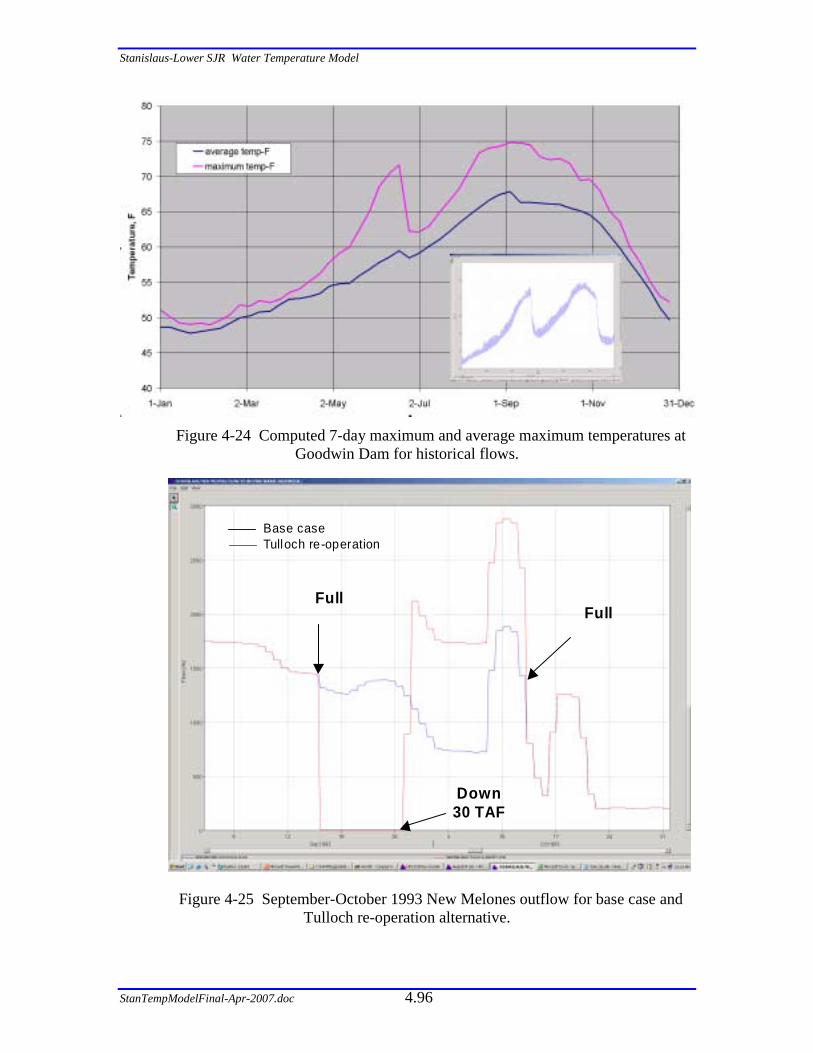
Stanislaus-Lower SJR Water Temperature Model
StanTempModelFinal-Apr-2007.doc 4.96
Figure 4-24 Computed 7-day maximum and average maximum temperatures at
Goodwin Dam for historical flows.
FullFull
Down 30 TAF
Base caseTulloch re-operation
Figure 4-25 September-October 1993 New Melones outflow for base case and Tulloch re-operation alternative.
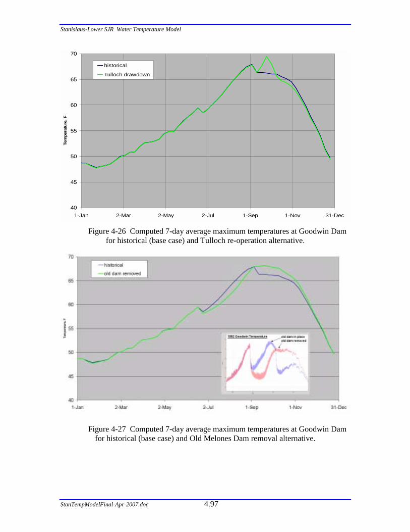
Stanislaus-Lower SJR Water Temperature Model
StanTempModelFinal-Apr-2007.doc 4.97
40
45
50
55
60
65
70
1-Jan 2-Mar 2-May 2-Jul 1-Sep 1-Nov 31-Dec
Tem
pera
ture
, Fhistorical
Tulloch drawdown
Figure 4-26 Computed 7-day average maximum temperatures at Goodwin Dam
for historical (base case) and Tulloch re-operation alternative.
Figure 4-27 Computed 7-day average maximum temperatures at Goodwin Dam
for historical (base case) and Old Melones Dam removal alternative.
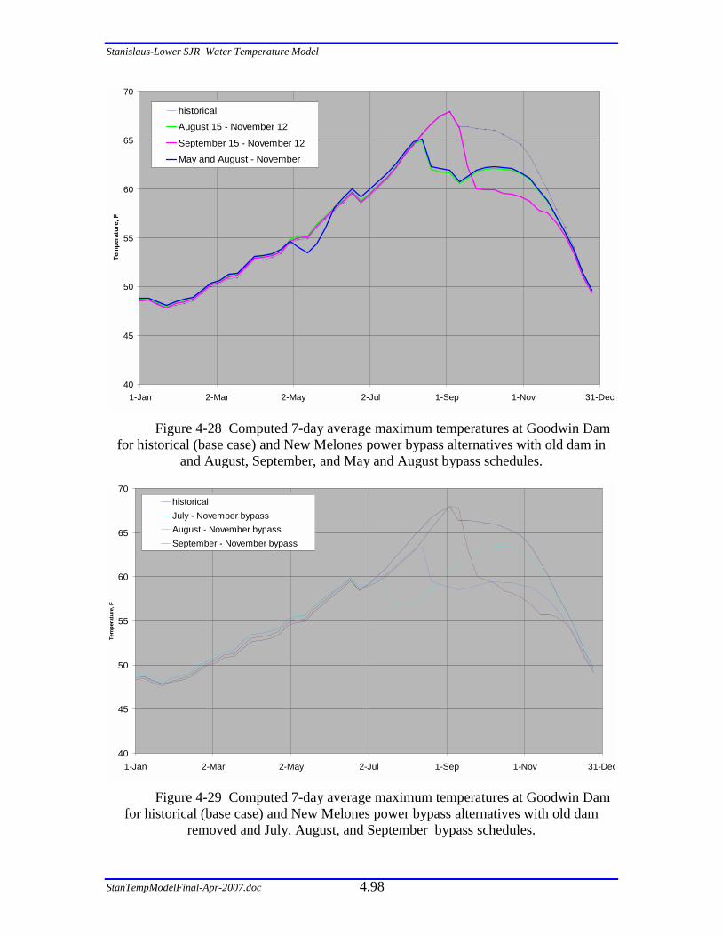
Stanislaus-Lower SJR Water Temperature Model
StanTempModelFinal-Apr-2007.doc 4.98
40
45
50
55
60
65
70
1-Jan 2-Mar 2-May 2-Jul 1-Sep 1-Nov 31-Dec
Tem
pera
ture
, Fhistorical
August 15 - November 12
September 15 - November 12
May and August - November
Figure 4-28 Computed 7-day average maximum temperatures at Goodwin Dam
for historical (base case) and New Melones power bypass alternatives with old dam in and August, September, and May and August bypass schedules.
40
45
50
55
60
65
70
1-Jan 2-Mar 2-May 2-Jul 1-Sep 1-Nov 31-Dec
Tem
pera
ture
, F
historicalJuly - November bypassAugust - November bypassSeptember - November bypass
Figure 4-29 Computed 7-day average maximum temperatures at Goodwin Dam
for historical (base case) and New Melones power bypass alternatives with old dam removed and July, August, and September bypass schedules.

Stanislaus-Lower SJR Water Temperature Model
StanTempModelFinal-Apr-2007.doc 4.99
USGS 11300500 S SAN JOAQUIN CN NR KNIGHTS FERRY CA1/1/1917 - 9/30/2004
Max Daily Flow = 1320 CFS
0
100
200
300
400
500
600
700
800
900
1000
1100
1200
1300
1400
Jan-
17
Sep-
19
Jun-
22
Mar
-25
Dec
-27
Sep-
30
Jun-
33
Mar
-36
Nov
-38
Aug
-41
May
-44
Feb-
47
Nov
-49
Aug
-52
May
-55
Jan-
58
Oct
-60
Jul-6
3
Apr
-66
Jan-
69
Oct
-71
Jul-7
4
Mar
-77
Dec
-79
Sep-
82
Jun-
85
Mar
-88
Dec
-90
Aug
-93
May
-96
Feb-
99
Nov
-01
Aug
-04
Dai
ly F
low
in C
FS
Figure 4-30 Historical Flows in the SSJID/OID Joint Canal
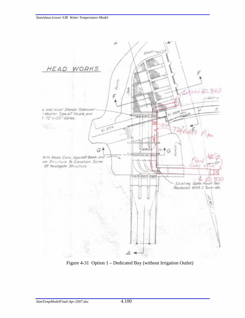
Stanislaus-Lower SJR Water Temperature Model
StanTempModelFinal-Apr-2007.doc 4.100
Figure 4-31 Option 1 – Dedicated Bay (without Irrigation Outlet)
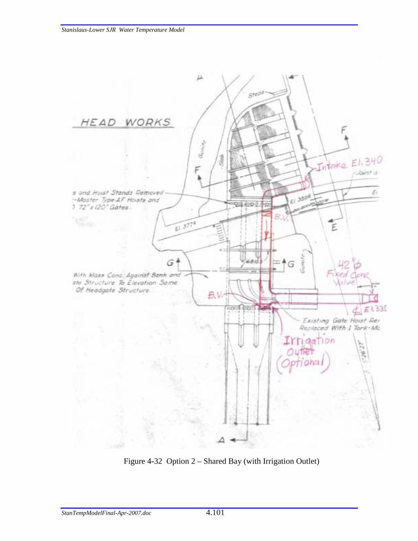
Stanislaus-Lower SJR Water Temperature Model
StanTempModelFinal-Apr-2007.doc 4.101
Figure 4-32 Option 2 – Shared Bay (with Irrigation Outlet)
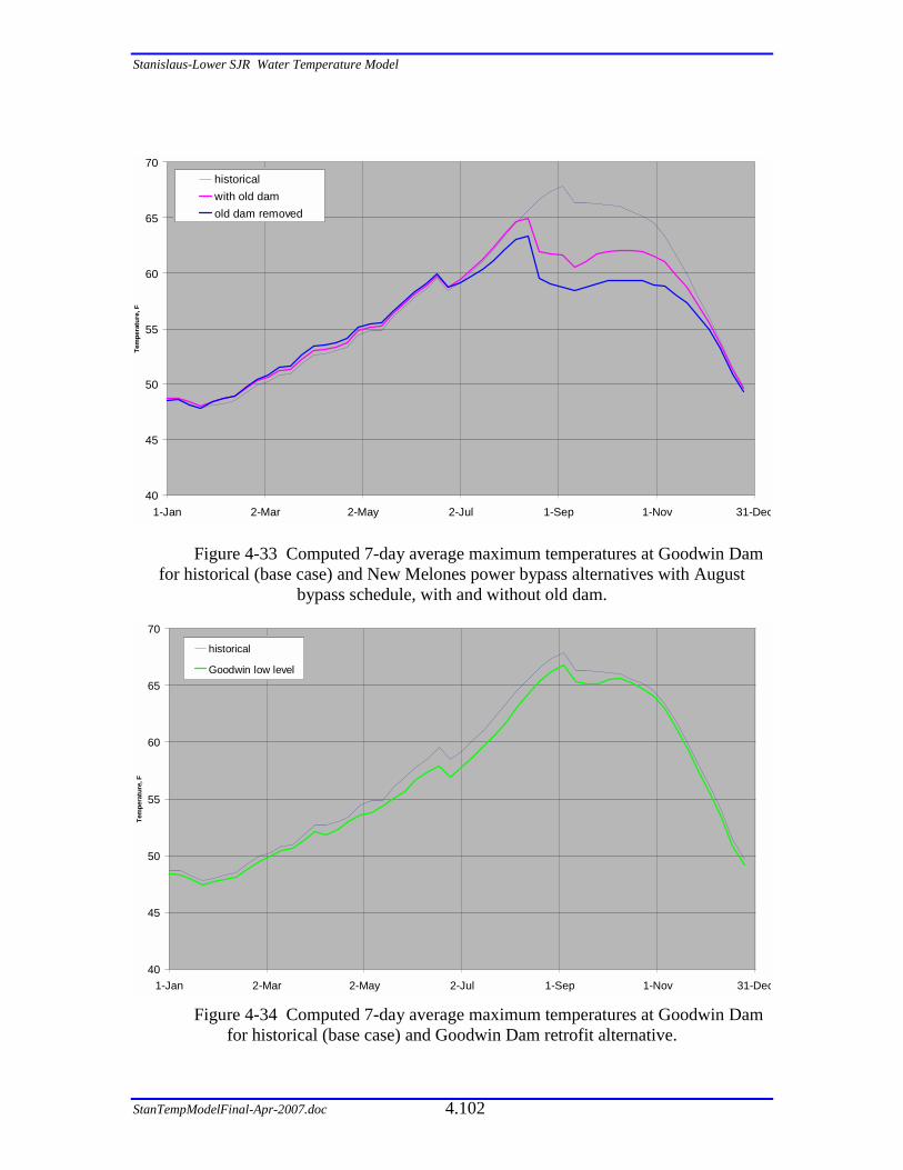
Stanislaus-Lower SJR Water Temperature Model
StanTempModelFinal-Apr-2007.doc 4.102
40
45
50
55
60
65
70
1-Jan 2-Mar 2-May 2-Jul 1-Sep 1-Nov 31-Dec
Tem
pera
ture
, F
historicalwith old damold dam removed
Figure 4-33 Computed 7-day average maximum temperatures at Goodwin Dam for historical (base case) and New Melones power bypass alternatives with August
bypass schedule, with and without old dam.
40
45
50
55
60
65
70
1-Jan 2-Mar 2-May 2-Jul 1-Sep 1-Nov 31-Dec
Tem
pera
ture
, F
historical
Goodwin low level
Figure 4-34 Computed 7-day average maximum temperatures at Goodwin Dam
for historical (base case) and Goodwin Dam retrofit alternative.

Stanislaus-Lower SJR Water Temperature Model
StanTempModelFinal-Apr-2007.doc 4.103
( )
40
45
50
55
60
65
70
1-Jan 2-Mar 2-May 2-Jul 1-Sep 1-Nov 31-Dec
Tem
pera
ture
, Fhistorical725 - 875 Selective withdrawaltailwater target temperatureSeptember bypass
Figure 4-35 Computed 7-day average maximum temperatures at Goodwin Dam
for historical (base case) and New Melones 725’-875’ selective withdrawal alternative with old dam. Tailwater target temperatures and New Melones September power bypass
alternative with old dam in are plotted for comparison. ( )
40
45
50
55
60
65
70
1-Jan 2-Mar 2-May 2-Jul 1-Sep 1-Nov 31-Dec
Tem
pera
ture
, F
no bypass or selective withdrawal
Selective withdrawal
tailwater target temperature
September - November bypass
Figure 4-36 Computed 7-day average maximum temperatures at Goodwin Dam
for: Old dam removed with no other changes; New Melones 675’-875’ selective withdrawal alternative with old dam removed; and New Melones September power
bypass alternative with old dam removed.

Stanislaus-Lower SJR Water Temperature Model
StanTempModelFinal-Apr-2007.doc 5.104
40
45
50
55
60
65
70
1-Jan 2-Mar 2-May 2-Jul 1-Sep 1-Nov 31-Dec
Tem
pera
ture
, Fhistorical
dam lowered 50ft and power extendedpower extended: August bypass
Figure 4-37 Computed 7-day average maximum temperatures at Goodwin Dam
for historical (base case), Old Melones Dam lowered 50’ with power intake lowered 100’, and power intake lowered 100’ with New Melones September power bypass.
40
45
50
55
60
65
70
1-Jan 2-Mar 2-May 2-Jul 1-Sep 1-Nov 31-Dec
Tem
pera
ture
, F
historicalwith old damold dam removedold dam partial removed
Figure 4-38 Computed 7-day average maximum temperatures at Goodwin Dam
for historical (base case), and New Melones September power bypass alternative with old dam in, with complete removal of old dam, and with partial removal of old dam.
5
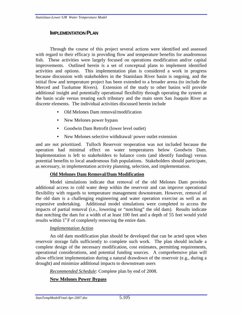
Stanislaus-Lower SJR Water Temperature Model
StanTempModelFinal-Apr-2007.doc 5.105
IMPLEMENTATION PLAN
Through the course of this project several actions were identified and assessed with regard to their efficacy in providing flow and temperature benefits for anadromous fish. These activities were largely focused on operations modification and/or capital improvements. Outlined herein is a set of conceptual plans to implement identified activities and options. This implementation plan is considered a work in progress because discussion with stakeholders in the Stanislaus River basin is ongoing, and the initial flow and temperature project has been extended to a broader arena (to include the Merced and Tuolumne Rivers). Extension of the study to other basins will provide additional insight and potentially operational flexibility through operating the system at the basin scale versus treating each tributary and the main stem San Joaquin River as discrete elements. The individual activities discussed herein include
• Old Melones Dam removal/modification
• New Melones power bypass
• Goodwin Dam Retrofit (lower level outlet)
• New Melones selective withdrawal/ power outlet extension and are not prioritized. Tulloch Reservoir reoperation was not included because the operation had minimal effect on water temperatures below Goodwin Dam. Implementation is left to stakeholders to balance costs (and identify funding) versus potential benefits to local anadromous fish populations. Stakeholders should participate, as necessary, in implementation activity planning, selection, and implementation.
Old Melones Dam Removal/Dam Modification Model simulations indicate that removal of the old Melones Dam provides
additional access to cold water deep within the reservoir and can improve operational flexibility with regards to temperature management downstream. However, removal of the old dam is a challenging engineering and water operation exercise as well as an expensive undertaking. Additional model simulations were completed to access the impacts of partial removal (i.e., lowering or “notching” the old dam). Results indicate that notching the dam for a width of at least 100 feet and a depth of 55 feet would yield results within 1o F of completely removing the entire dam.
Implementation Action An old dam modification plan should be developed that can be acted upon when
reservoir storage falls sufficiently to complete such work. The plan should include a complete design of the necessary modification, cost estimates, permitting requirements, operational considerations, and potential funding sources. A comprehensive plan will allow efficient implementation during a natural drawdown of the reservoir (e.g., during a drought) and minimize additional impacts to downstream users
Recommended Schedule: Complete plan by end of 2008.
New Melones Power Bypass
Stanislaus-Lower SJR Water Temperature Model
StanTempModelFinal-Apr-2007.doc 5.106
Simulations identify improved temperature control flexibility, particularly in the fall, through bypassing the powerhouse at New Melones to access deeper, cooler waters. This activity can be implemented with existing infrastructure, but has an associated cost of foregone hydropower production.
Implementation Action Although initial estimates of foregone power through New Melones bypass are
identified earlier in this report, it is recommended that a more comprehensive study be completed to identify potential schedules and associated costs. These costs can be compared with potential biological benefits and refined as necessary (e.g., by year types, storage in New Melones, status of fishery, etc.).
Recommended Schedule: Complete feasibility/economic report by end of 2008.
Goodwin Bypass The Goodwin Bypass would provide a relatively low cost capital improvement to
thermal benefit in the Stanislaus River reach immediately below Goodwin Dam. The reach impacted by the operation would be relatively short, but is used by anadromous fish for nearly all life stages (i.e., spawning, egg incubation, juvenile rearing (including summer rearing).
Implementation Action Review and revise the initial design level calculations and costs for the retrofit.
Address institutional and permitting issues associated with this action. Pre- and post-monitoring should be included in the project. Subsequently develop a funding sources and acceptance of final design by appropriate stakeholders.
Recommended Schedule: Complete feasibility/economic report by end of 2008.
Selective Withdrawal/Power Extension Selective withdrawal, particularly with Old Melones dam modifications, can
provide operational flexibility with respect to temperature control in downstream river reaches while maintaining hydropower production at approximately current levels. In general, the power extension, to access cooler water, was less effective than selective withdrawal due to lack of operational flexibility. If modification of the outlet works to accommodate some type of deeper water withdrawal is desired, the recommendation is to use selective withdrawal versus a power extension. The power extension will not be discussed further. Any modification to outlet works is challenging from an engineering and system operations perspective, as well as costly.
Implementation Action Explore feasibility of selective withdrawal facilities through development of cost
estimates for construction, operation and maintenance, and hydropower production. Reference costs based on full pool construction (e.g., underwater construction) versus lowered pool construction. The report should yield critical insight to the costs and benefits of such a project. Consideration of the costs and benefits may be important to compare with future findings on the Merced and Tuolumne Rivers under the extended

Stanislaus-Lower SJR Water Temperature Model
StanTempModelFinal-Apr-2007.doc 6.107
project. Selective withdrawal may provide more specific benefits on the Tuolumne or Merced than on the Stanislaus from the basin-scale perspective.
Recommended Schedule: Complete feasibility report by end of 2008. Consider findings of extended project (i.e. Tuolumne and Merced Rivers) when setting final schedule.
5.1.1 Conclusion
Generally, there are multiple activities where action can occur immediately. Although several years have been identified to arrive at final reports for implementation activities, in some cases it may be prudent to accommodate information from the other river systems (Tuolumne and Merced) into the decision process. For this reason, this implementation plan does not identify a schedule for completion of activities. Further, with Reclamation ongoing activities in the basin in developing a revised long-term operation plan for New Melones Reservoir, it may be prudent to consider future changes in operations and conditions prior to embarking on certain aspects of this implementation plan. An encouraging aspect of this study is the continued, direct involvement of basin stakeholders in identifying potential actions and participating in the assessment of these actions. With continued stakeholder involvement, it is envisioned that acceptable actions will be appropriately studied and implemented as funding and need arise.
6 REFERENCES
Deas, M.L., J.Bartholow, C.Hanson, C. Myrick. 2004. Peer Review of Water Temperature Objectives Used as Evaluation Criteria for the Stanislaus – Lower San Joaquin River Water Temperature Modeling and Analysis: Task 9 Prepared fro AD Consultants. CBDA Project No.: ERP-02-P28. July 29. 54 pp.
Deas, M.L. 2001. “Appraisal of the Application of HEC-5Q for Temperature Simulation of the Stanislaus River,” Technical memorandum prepared for A-D Consultants by Watercourse Engineering, Napa CA., July 20.
Hydrologic Engineering Center (HEC). 1999b. Water Quality Modeling of Reservoir System Operations Using HEC-5, Training Document., U.S. Army Corps of Engineers, Hydrologic Engineering Center, Davis CA.
Hydrologic Engineering Center (HEC). 2000. HEC-5, Simulation of Flood Control and Conservation Systems, Appendix on Water Quality Analysis, U.S. Army Corps of Engineers, Hydrologic Engineering Center, Davis, CA.
Guignard, J., 2001. Stanislaus River Temperature Monitoring/Modeling Project Water Temperature Criteria Development. California Department of Fish and Game. January 17.
United States Environmental Protection Agency (EPA). 2003. EPA Region 10 Guidance for Pacific Northwest State and Tribal Temperature Water Quality Standards. EPA 910-B-03-002. April. 49 pp.
Stanislaus-Lower SJR Water Temperature Model
StanTempModelFinal-Apr-2007.doc 7.108
7 ATTACHMENTS
The following is a list of relevant material included in the attached compact disk:
7.1 DATA COLLECTION PROTOCOL
• For the Lower San Joaquin River Basin – Wide Water Temperature Modeling Project Data Collection Protocol, developed by the CDFG, see attached file:
ProjectPlan082206.pdf
7.2 PEER REVIEW REPORTS
• For the Peer Review Report for Water Temperature Objectives Used as Evaluation Criteria for the Stanislaus-Lower San Joaquin River Water Temperature Modeling and Analysis, see attached file:
StanislausTemperaturePeerReviewFinal.pdf
• For the Memorandum Re: Peer Review Panel – Expansion of Thermal Criteria to the Greater San Joaquin River Basin, see attached file:
MEMORANDUM8-23-06.pdf
7.3 LETTERS COMMENTS FROM STANISLAUS STAKEHOLDERS
7.3.1 Oakdale ID, South San Joaquin ID, Stockton East WD and Tri-Dam
• For the Oakdale Irrigation District, South San Joaquin Irrigation District, Stockton East Water District, and Tri-Dam comments regarding the overall project and proposed water temperature management plans in the Stanislaus River, see attached files:
TEMPERATURE.M102306.MODELING.pdf Memo121306final.pdf
7.3.2 California Department of Fish and Game
• For the California Department of Fish and Game comments regarding the overall project and proposed water temperature management plans in the Stanislaus River, see attached files:
DraftSRTempModelRpt_CDFGLetter.pdf FinalRptCDFGCommentLetter040907.pdf
Stanislaus-Lower SJR Water Temperature Model
StanTempModelFinal-Apr-2007.doc 8.109
7.4 LETTERS COMMENTS FROM TUOLUMNE & MERCED STAKEHOLDERS
7.4.1 Merced ID
• For the Merced Irrigation District comments regarding the Memorandum Re: Peer Review Panel – Expansion of Thermal Criteria to the Greater San Joaquin River Basin, see attached file:
VogelCommentsonTemperatureMemo.pdf
7.4.2 Turlock ID and Modesto ID
• For the Turlock Irrigation District and Modesto Irrigation District comments regarding the Memorandum Re: Peer Review Panel – Expansion of Thermal Criteria to the Greater San Joaquin River Basin, see attached file:
Avry06Oct2006_1.pdf
7.5 GOODWIN RETROFIT – COST ESTIMATE
• For the Goodwin Retrofit pre-feasibility Report, see attached file:
Pre-feasibilityGoodwinRetro.pdf
8 COMPACT DISK CONTENT
The attached Compact Disk contains a letter transmittal to GCAP and CALFED letterGCAP&CALFED-4-19-07.doc and three main directories: HWMS, REPORT and SJT&SRT. The content of each directory is as follows:
8.1 HWMS (HYDROLOGIC WATER-QUALITY MODELING SYSTEM)
This directory includes four files:
1. HWMS_StartUp.doc 2. HWMS_Setup.exe 3. HWMS_Users_Manual.doc 4. J2re_1_5_0_8-windows_i586-p.exe
The HWMS_StartUp.doc has all the information needed in order to install the HWMS (including the model’s executable, input and output files) and view the Stanislaus-Lower San Joaquin River HEC-5Q model results. It also describes the content of the other three files in that directory.
Stanislaus-Lower SJR Water Temperature Model
StanTempModelFinal-Apr-2007.doc 8.110
8.2 REPORT
This directory includes the project final report (this document) StanTempModelFinal-Apr-2007.pdf and a sub-directory called ATTACHMENTS.
8.2.1 ATTACHMENTS
This sub-directory contains all the files referenced in Section 7:
1. ProjectPlan082206.pdf 2. StanislausTemperaturePeerReviewFinal.pdf 3. MEMORANDUM8-23-06.pdf 4. TEMPERATURE.M102306.MODELING.pdf 5. Memo121306final.pdf 6. DraftSRTempModelRpt_CDFGLetter.pdf 7. FinalRptCDFGCommentLetter040907.pdf 8. VogelCommentsonTemperatureMemo.pdf 9. Avry06Oct2006_1.pdf 10. Pre-feasibilityGoodwinRetro.pdf
8.3 SJT&SRT
This directory includes the updated temperature databases:
1. SJT db102506.mdb – Tuolumne/Merced/San Joaquin River 2. SRT db102306.mdb – Stanislaus River