standard port-visit cost forecasting model for u.s. navy ... · pdf filestandard port-visit...

Calhoun: The NPS Institutional Archive

Theses and Dissertations Thesis Collection

2009-12

Standard port-visit cost forecasting model for U.S.

Navy husbanding contracts

Marquez, Michael Alvin A.

Monterey, California: Naval Postgraduate School

http://hdl.handle.net/10945/10412

NAVAL POSTGRADUATE

SCHOOL

MONTEREY, CALIFORNIA

MBA PROFESSIONAL REPORT

Standard Port-Visit Cost Forecasting Model

For U.S. Navy Husbanding Contracts

By: Michael Alvin A. Marquez, Richard M. Rayos, and John I. Mercado

December 2009

Advisors: Raymond Franck Brett Wagner Douglas Brinkley

Approved for public release; distribution is unlimited

THIS PAGE INTENTIONALLY LEFT BLANK

i

REPORT DOCUMENTATION PAGE Form Approved OMB No. 0704-0188 Public reporting burden for this collection of information is estimated to average 1 hour per response, including the time for reviewing instruction, searching existing data sources, gathering and maintaining the data needed, and completing and reviewing the collection of information. Send comments regarding this burden estimate or any other aspect of this collection of information, including suggestions for reducing this burden, to Washington headquarters Services, Directorate for Information Operations and Reports, 1215 Jefferson Davis Highway, Suite 1204, Arlington, VA 22202-4302, and to the Office of Management and Budget, Paperwork Reduction Project (0704-0188) Washington DC 20503.

1. AGENCY USE ONLY (Leave blank)

2. REPORT DATE December 2009

3. REPORT TYPE AND DATES COVERED MBA Professional Report

4. TITLE AND SUBTITLE Standard Port-Visit Cost Forecasting Model for U.S. Navy Husbanding Contracts

6. AUTHOR(S) Michael Alvin A. Marquez, Richard M. Rayos, & John I. Mercado

5. FUNDING NUMBERS

7. PERFORMING ORGANIZATION NAME(S) AND ADDRESS(ES) Naval Postgraduate School Monterey, CA 93943-5000

8. PERFORMING ORGANIZATION REPORT NUMBER

9. SPONSORING /MONITORING AGENCY NAME(S) AND ADDRESS(ES) N/A

10. SPONSORING/MONITORING AGENCY REPORT NUMBER

11. SUPPLEMENTARY NOTES The views expressed in this thesis are those of the authors and do not reflect the official policy or position of the Department of Defense or the U.S. Government.

12a. DISTRIBUTION / AVAILABILITY STATEMENT Approved for public release; distribution is unlimited

12b. DISTRIBUTION CODE A

13. ABSTRACT (maximum 200 words) Husbanding services are crucial elements of a port visit. In support of mission objectives, combatant commanding officers and sealift masters rely on contractors to act on the U.S. Navy’s behalf in coordinating the delivery of supplies or performance of services. Through the years, the cost of port services around the world has increased in various magnitudes. However, the U.S. Navy’s ability to track and analyze port-visit costs changes remains rudimentary. Current systems lack the functionality needed by the stakeholders to effectively and efficiently forecast port-visit costs.

The researchers developed a Web-based modularized application that stores and displays invoices, generates reports, and more importantly, forecasts future port-visit costs using the standard port-visit cost forecasting model for husbanding contracts. The forecasting function of the application provides two predictive methods, namely confidence interval estimator and exponential smoothing. The analysis clearly shows that low requirement variability improves the reliability of the interval, while high frequency of port-visits increases the accuracy of the exponential smoothing results. The capabilities of the application provide stakeholders with a valuable tool to analyze port-visit requirements and costs trends.

15. NUMBER OF PAGES

119

14. SUBJECT TERMS Husbanding Services, Standard Port-visit Cost Forecasting Model, Husbanding Service Provider, Port-Visit Cost Reports, LOGREQ, CRAFT, WWCRAFT, LogSSR, LOGCOP, COMFISCS, FISCs, CLASSRON, TYCOMS, NAVSUP 16. PRICE CODE

17. SECURITY CLASSIFICATION OF REPORT

Unclassified

18. SECURITY CLASSIFICATION OF THIS PAGE

Unclassified

19. SECURITY CLASSIFICATION OF ABSTRACT

Unclassified

20. LIMITATION OF ABSTRACT

UU

Standard Form 298 (Rev. 2-89) Prescribed by ANSI Std. 239-18

ii


iii

Approved for public release; distribution is unlimited

STANDARD PORT-VISIT COST FORECASTING MODEL FOR U.S. NAVY HUSBANDING CONTRACTS

Michael Alvin A. Marquez, Lieutenant Commander, United States Navy Richard M. Rayos, Lieutenant Commander, United States Navy

John I. Mercado, Lieutenant, United States Navy

Submitted in partial fulfillment of the requirements for the degree of

MASTER OF BUSINESS ADMINISTRATION

from the

NAVAL POSTGRADUATE SCHOOL December 2009

Authors: _____________________________________

Michael Alvin A. Marquez _____________________________________

Richard M. Rayos _____________________________________

John I. Mercado

Approved by: _____________________________________

Raymond Franck, Lead Advisor _____________________________________

Brett Wagner, Support Advisor _____________________________________ Douglas Brinkley, Support Advisor _____________________________________ William Gates, Dean

Graduate School of Business and Public Policy

iv


v

STANDARD PORT-VISIT COST FORECASTING MODEL FOR U.S. NAVY HUSBANDING CONTRACTS

ABSTRACT

Husbanding services are crucial elements of a port visit. In support of mission

objectives, combatant commanding officers and sealift masters rely on contractors to act

on the U.S. Navy’s behalf in coordinating the delivery of supplies or performance of

services. Through the years, the cost of port services around the world has increased in

various magnitudes. However, the U.S. Navy’s ability to track and analyze port-visit cost

changes remains rudimentary. Current systems lack the functionality needed by the

stakeholders to effectively and efficiently forecast port-visit costs.

The researchers developed a Web-based modularized application that stores and

displays invoices, generates reports, and more importantly, forecasts future port-visit

costs using the standard port-visit cost forecasting model for husbanding contracts. The

forecasting function of the application provides two predictive methods, namely

confidence interval estimator and exponential smoothing. The analysis clearly shows that

low requirement variability improves the reliability of the interval, while high frequency

of port-visits increases the accuracy of the exponential smoothing results. The

capabilities of the application provide stakeholders with a valuable tool to analyze port-

visit requirements and costs trends.

vi


vii

TABLE OF CONTENTS

I. INTRODUCTION........................................................................................................1

II. BACKGROUND ..........................................................................................................5 A. CURRENT RESOURCE TOOLS AVAILABLE, AND THEIR

LIMITATIONS.................................................................................................6 1. Legacy Cost Reporting, Analysis and Forecasting Tool

(CRAFT) ...............................................................................................6 a. LOGREQ Initial Cost Estimate ................................................7 b. Actual Cost Report ....................................................................7

2. Worldwide Cost-Reporting, Analysis and Forecasting Tool (WWCRAFT)........................................................................................8 a. LOGREQ Initial Cost Estimate ................................................8 b. Actual Cost Report ....................................................................9

3. Logistics Support Services Repository (LogSSR) ...........................10 4. Logistic Common Operating Picture (LOGCOP) ..........................12

B. STANDARD PORT-VISIT COST FORECASTING MODEL (SPCFM) CAPABILITIES AND LIMITATIONS .....................................12

C. BACKGROUND SUMMARY......................................................................13

III. LITERATURE REVIEW .........................................................................................15 A. HUSBANDING SERVICE PROVIDER (HSP) CONCEPT .....................15 B. DEFINITION OF A HUSBANDING CONTRACT...................................16 C. COMFISCS’ WORLDWIDE HUSBANDING CONTRACT

COVERAGE ..................................................................................................16 D. COMFISCS GLOBAL HUSBANDING INITIATIVES AT VARIOUS

FISCS ..............................................................................................................19 1. FISC Norfolk ......................................................................................19 2. FISC San Diego ..................................................................................20 3. FISC Sigonella....................................................................................20 4. FISC Yokosuka ..................................................................................21

E. FUTURE OF HUSBANDING SERVICE PROVIDER (HSP) CONTRACTS ................................................................................................22

F. HUSBANDING SERVICE PROVIDER RESPONSIBILITIES...............23 1. Advance Party ....................................................................................23 2. Ship’s Logistic Requirements (LOGREQ) ......................................23 3. Initial Boarding ..................................................................................24

G. SERVICES ARRANGED BY THE HUSBANDING SERVICE PROVIDER ....................................................................................................24 1. Husbanding Services Fee...................................................................24 2. Trash Removal ...................................................................................24 3. Collection, Holding, and Transfer (CHT)/Sewage Removal..........25 4. Yokohama or Comparable-Type Fenders .......................................25 5. Fresh, Potable Water .........................................................................26

viii

6. Pilots, Tug Services, and Line Handlers ..........................................26 7. Water Ferry / Taxi Services ..............................................................26 8. Transportation Service......................................................................27

a. Bus Service ..............................................................................27 b. Vehicle Rental Service ............................................................27

9. Force Protection Services and Supplies ...........................................27 10. Camels.................................................................................................28 11. Landing Barges ..................................................................................28 12. Fleet Landing......................................................................................28 13. Provisions............................................................................................28 14. Oily Waste Removal ..........................................................................28

IV. PROJECT WEB-BASED APPLICATION.............................................................31 A. STANDARDIZATION..................................................................................31 B STANDARD PORT-VISIT COST FORECASTING MODEL

(SPCFM) .........................................................................................................32 C. ORIGIN OF DATA........................................................................................32 D. SYSTEM ENVIRONMENT .........................................................................33 E. IMPLEMENTATION OF FUNCTIONS ....................................................33

1. Administrative Tools .........................................................................34 2. Data Security ......................................................................................36 3. Display Invoices..................................................................................37 4. Generating Reports............................................................................38 5. Forecasting..........................................................................................41

F. SAME VESSEL TYPE, SAME PORT, SAME COUNTRY .....................43 G. SAME VESSEL CLASS, SAME PORT, SAME COUNTRY ...................43 H. NOT THE SAME VESSEL TYPE/CLASS, SAME PORT, SAME

COUNTRY......................................................................................................43 I. NOT THE SAME VESSEL TYPE/CLASS, NOT THE SAME PORT,

SAME COUNTRY.........................................................................................44 J. NOT THE SAME COUNTRY; ONLY INVOICES FROM OTHER

COUNTRIES ARE AVAILABLE................................................................44

V. FORECASTING METHODOLOGY ......................................................................45 A. CONFIDENCE INTERVAL ESTIMATOR ...............................................45

1. Select Parameters...............................................................................45 2. Get Historical Data ............................................................................45

3. Critical Values of Student t-distribution ( /2t )..............................46

4. Adjust Invoice Item per Day Quantity.............................................46

5. Get the Sub-CLIN Type Average ( x ) ..............................................47

6. Get the Variance and Standard Deviation ( 2 &s s ) ...................49

7. Get the Sub-CLIN Type Confidence Interval ( /2

st

n ).................50

B. EXPONENTIAL SMOOTHING..................................................................51 1. Do Exponential Smoothing (Forecast[t+1]) .....................................52

ix

2. Find the Optimal Smoothing Constant ()......................................53

VI. ANALYSIS .................................................................................................................59 A. CASE ANALYSIS..........................................................................................60

1. Two Ship Types Anchored at Port Red, Country Alpha ...............60 a. DDG at Anchor .......................................................................60 b. CG at Anchor ..........................................................................62

2. Two Ship Types at Different Ports in the Same Country...............64 a. TAO Visiting Pier Side of Port Orange, Country Bravo .......64 b. DDG Visiting Pier Side of Port Yellow, Country Bravo........66

3. A Different Class of Ship Visiting Pierside......................................68 4. Two Different Classes of Ships Visiting Multiple Ports in the

Same Country.....................................................................................69 a. LHD (Class 4 ship) Moored Pier Side at Port Indigo,

Country Delta. .........................................................................70 b. SSN (Class 1 Ship) Moored Pier Side at Port Blue,

Country Delta ..........................................................................71 B. SYNTHESIS ...................................................................................................73 C. CHAPTER SUMMARY................................................................................75

VII. CONCLUSION ..........................................................................................................77 A. SPCFM PERFORMANCE ...........................................................................77 B. DATA QUALITY...........................................................................................78 C. IMPACT TO STAKEHOLDERS ................................................................79

VIII. RECOMMENDATIONS...........................................................................................81 A. STANDARDIZE THE CLIN STRUCTURE OF HUSBANDING

SERVICES CONTRACTS ...........................................................................81 B. ADD A FORECASTING FUNCTIONALITY INTO EXISTING

DATA REPOSITORY APPLICATIONS....................................................81 C. ASSIGN A LEAD OFFICE RESPONSIBLE FOR ASSIGNING

NEW, UNIQUE CLIN IDENTIFIERS........................................................82 D. USE ONE DATA REPOSITORY FOR ALL HUSBANDING

CONTRACTS ................................................................................................82 E. TRAIN HSPS IN DATA ENTRY.................................................................83 F. INFORM THE FLEET THAT THE TOOL EXISTS................................83 G. AUDIT AND MONITOR THE INFORMATION IN THE DATA

REPOSITORY ...............................................................................................83

IX. AREAS FOR FURTHER RESEARCH...................................................................85 A. EXPAND THE FORECASTING MODEL TO INCLUDE

SCENARIOS II THROUGH V ....................................................................85 B. INTEGRATION OF GLOBAL HUSBANDING SERVICES WITH

NETWORK-CENTRIC LOGISTICS SYSTEMS......................................85

LIST OF REFERENCES......................................................................................................87

x

APPENDIX CASE DATA....................................................................................................89

INITIAL DISTRIBUTION LIST .........................................................................................97

xi

LIST OF FIGURES

Figure 1. Flow chart of HSP ordering process. (From King, 2009 January 30) ...............6 Figure 2. Gantt chart showing LogSSR development. (From King, 2009a, June 9). .....11 Figure 3. System comparison of CRAFT, WWCRAFT, LogSSR. (From King,

2009a, June 9). .................................................................................................11 Figure 4. Standard Port-visit Cost Forecasting Model Objective to Augment

Capabilities of LogSSR and LOGCOP............................................................13 Figure 5. Example of the CLIN structure used in the module. .......................................35 Figure 6. Description of the four access levels implemented in the module...................36 Figure 7. Screenshot of a portcall visit invoice. ..............................................................38 Figure 8. Screenshot of report selection..........................................................................39 Figure 9. Screenshot of fund code report. .......................................................................40 Figure 10. Screenshot of forecasting parameters. .............................................................41 Figure 11. Screenshot of a port-visit cost estimate. ..........................................................42

Figure 12. .025t Critical values (95% confidence level)....................................................46

Figure 13. “Adjust invoice item per day quantity” pseudo-code. .....................................47 Figure 14. Sub-CLIN type average pseudo-code. .............................................................48 Figure 15. Standard deviation pseudo-code. .....................................................................49 Figure 16. Confidence level pseudo-code. ........................................................................50 Figure 17. Exponential smoothing pseudo-code. ..............................................................53 Figure 18. Example of method iteration in search of the lowest MAPE...........................54 Figure 19. Pseudo-code for the generating the smoothing constant..................................55 Figure 20. The heuristic method pseudo-code. .................................................................56 Figure 21. Graph of 2008–2009 DDG Actual Port-visit Costs Compared to the

Forecasted Costs, Port Red, Country Alpha. ...................................................61 Figure 22. Graph of 2008–2009 DDG Estimate and Exponential Smoothing..................62 Figure 23. Graph of 2008–2009 CG Actual Port-visit Costs Compared to the

Forecasted Costs, Port Red, Country Alpha. ...................................................63 Figure 24. Graph of 2008–2009 CG Estimate and Exponential- smoothing Error Rate...63 Figure 25. Graph of 2008–2009 TAO Actual Port-visit Costs Compared to the

Forecasted Costs, Port Orange, Country Bravo. ..............................................64 Figure 26. Graph of 2008–2009 TAO Estimate and Exponential- smoothing Error

Rate. .................................................................................................................66 Figure 27. Graph of 2008–2009 DDG Actual Port-visit Costs Compared to the

Forecasted Costs, Port Yellow, Country Bravo. ..............................................66 Figure 28. Graph of 2008–2009 DDG Estimate and Exponential- smoothing Error

Rate. .................................................................................................................67 Figure 29. Graph of 2008–2009 LPD Actual Port-visit Costs Compared to the

Forecasted Costs, Port Green, Country Charlie. ..............................................68 Figure 30. Graph of 2008–2009 DDG Estimate and Exponential- smoothing Error

Rate. .................................................................................................................69

xii

Figure 31. Graph of the Estimates and Actual Port-visit Costs of LHD Visiting Port Indigo, Country Delta. .....................................................................................70

Figure 32. Graph of 2008–2009 DDG Estimate and Exponential- smoothing Error Rate. .................................................................................................................71

Figure 33. Graph of the Estimates and Actual Port-visit Costs of SSNs Visiting Port Blue, Country Delta. ........................................................................................72

Figure 34. Graph of 2008–2009 SSN Estimate and Exponential smoothing Error Rate. .................................................................................................................72

Figure 35. Synthesis Cube of Port-visit Costs...................................................................75

xiii

LIST OF TABLES

Table 1. Navy Regions and Operational Areas (After NAVSUP, 2009a).....................17 Table 2. List of TAO Port Visits that Incurred Actual Costs Beyond Upper

Boundary..........................................................................................................65 Table 3. Comparison of Error Rates, Exponential-smoothing vs. Estimate. .................74

xiv


xv

LIST OF ACRONYMS AND ABBREVIATIONS

ACO Administrative Contracting Officer

AOR Area of Responsibility

C3F Commander, Third Fleet

C3M Consolidate Husbanding Contract located in Canada, Caribbean, Central America, Mexico, and South America

CDR Commander

CENTCOM AOR Central Command Area of Responsibility

CG Guided Missile Cruisers

CHT Collection, Holding and Transfer

CLASSRON Class Squadron

CLIN Contract Line Item Number

CMP Continuous Monitoring Program

CNO Chief of Naval Operation

COMFISCS Commander, Fleet and Industrial Supply Centers

CONUS Continental United States

CPF Commander Pacific Fleet

CRAFT Legacy Cost Reporting, Analysis & Forecasting Tool

DDG Guided Missile Destroyer

DoD Department of Defense

ELRT Expeditionary Logistics Response Teams

EUCOM United States European Command

FAR Federal Acquisition Regulation

FFG Guided Missile Frigate

FFP-IDTC Firm-Fixed Price Indefinite Delivery Type Contract

FFV Fresh Fruits and Vegetables

FISCs Fleet and Industrial Supply Centers

FISCSD Fleet and Industrial Supply Center San Diego

FISCSI Fleet and Industrial Supply Center Sigonella

FISCY Fleet Industrial Supply Center Yokosuka

HSP Husbanding Service Provider

xvi

HTTP Hypertext Transfer Protocol

IP Internet Protocol

ISS Inchcape Shipping Services

IT Information Technology

KO Contracting Officer

LHD Multi-Purpose Landing Helicopter Dock

LOGCOP Logistic Common Operating Picture

LOGREQ Logistical Requirements

LogSRR Logistics Support Services Repository

LPD Landing Platform Dock

MAPE Mean Absolute Percentage of Error

MLS Multinational Logistics Services

MySQL My Structured Query Language

NAVSUP Navy Supply Systems Command

NC Non-Contract Items

NPS Naval Postgraduate School

NRCD Navy Regional Contracting Detachment

OCONUS Outside Continental United States

OOTW Operations Other Than War

PAT Process Action Team

PCO Procurement Contracting Officer

PHP Hypertext Preprocessor

PKI Public Key Infrastructure

PVCR Port-Visit Cost Reports

RADM Rear Admiral

SOW Statement of Work

SPCFM Standard Port-visit Cost Forecasting Model

SSN Fast Attack Submarine (Nuclear)

SUPPO Supply Officer

TAO Fleet Replenishment Oilers

TYCOMS Type Commanders

UAE United Arab Emirates

xvii

UK United Kingdom

US United States

WWCRAFT Worldwide Cost Reporting, Analysis, and Forecasting Tool

xviii


xix

ACKNOWLEDGMENTS

We would like to thank our spouses for their tremendous support during the

writing of this MBA Project. We cannot extend enough appreciation and thanks for the

continued understanding and flexibility throughout the long hours dedicated to this

project.

We would also like to thank the major contributors at PACFLEET, C3F,

COMFISCS, CNSF, and NAVSUP 02, especially LCDR Jerry King, who generously

provided us with data, insights, and answers to our numerous inquiries during the conduct

of our research.

Additionally, we would like to thank the Acquisition Research Program,

especially RADM James Green, USN (Ret), Ms. Karey Shaffer, and Ms. Tera Yoder, for

providing the necessary funding and resources that brought this MBA Project together.

Furthermore, we are also grateful to the Thesis Processing Center, particularly Ms. Susan

Hawthorne, for her assistance and support.

Finally, we would like to thank Brig. Gen. Raymond Franck, USAF (Ret), PhD,

CDR Brett Wagner, SC, USN, and Dr. Douglas Brinkley, EdD, for their wisdom and

guidance during the writing of this MBA Project.

xx


1

I. INTRODUCTION

Husbanding services are crucial elements of a port visit. In support of mission

objectives, combatant commanding officers and sealift masters rely on contractors to act

on the U.S. Navy’s behalf in coordinating the delivery of supplies or the performance of

services. Through the years, the cost of port services around the world has increased in

various magnitudes. However, the Navy’s ability to track and analyze port-visit cost

changes remains rudimentary, since current systems lack the functionality needed by the

stakeholders to effectively and efficiently forecast port-visit costs. This project focuses

on developing and testing the Standard Port-visit Cost Forecasting Model (SPCFM), a

Web-based forecasting application, designed to enhance current system capabilities and

predict port-visit costs.

The high-level echelons, such as Navy Supply Systems Command (NAVSUP)1,

Type Commanders (TYCOMs),2 Fleet Commanders,3 and Class Squadron

(CLASSRON),4 have long desired improvements on predicting port-visit cost through

better forecasting. For the numbered Fleet Commanders, the biggest challenge relates to

projecting the budget of port-visit costs. As of this year, TYCOMs delegated the

management of port visits to the numbered Fleet Commanders. Prior to delegating the

management function, TYCOMs managed the cost of port visits while the Fleet

Commanders wrote the messages tasking ships to visit specific ports. Now, TYCOMs

gives each of the Fleet Commanders a budgeted amount to allocate among several port

visits.

1 NAVSUP manages supply chains that provide material for Navy aircraft, surface ships, submarines

and their associated weapon systems.

2 Type Commanders control ships within a type category. Aircraft carriers, aircraft squadrons, and air stations are under the administrative control of the appropriate Commander Naval Air Force. Submarines come under the Commander Submarine Force. All other ships fall under Commander Naval Surface Force.

3 The U.S. Navy is currently organized into five fleets: Second Fleet in the Atlantic, Third Fleet in the Eastern Pacific, Fifth Fleet in the Arabian Gulf and Indian Ocean, Sixth Fleet in the Mediterranean, and Seventh Fleet in the Western Pacific.

4 CLASSRON analyze metrics across ships of a class, access current readiness and cost control processes.

2

During a site visit to Third Fleet, the researchers learned that the Third Fleet N4

had to rely on locally developed spreadsheets and available information from LOGCOP

(Logistic Common Operating Picture)5 to validate the feasibility of a port visit based on

current budget constraints. Therefore, Fleet Commanders are very interested in a port-

visit cost forecasting tool for their strategic operational planning (C3F N4A, 2009).

On a ship level, one of the many challenging responsibilities of a ship’s Supply

Officer (SUPPO) during a deployment is coordinating the ship’s port visit support with

the Husbanding Service Provider (HSP)6. The support and cost vary depending on the

geographical location, the ship’s mission, and resources available in the region (Hall &

Adams, 2007). The SUPPO needs such a forecasting tool to help assess a ship’s

upcoming port-visit cost. Currently, existing systems do not have the capability to

forecast and assist in mitigating costs. This project provides a cost-estimating module

that supply officers could use in projecting the cost of an upcoming port visit.

The process of developing the application includes collecting a four-year data set

of invoices, from 2006 to 2009. Prior to populating the database, the project team

members developed, debugged, and tested the Web-based application. Due to Contract

Line Item Number (CLIN) discrepancies, which will be discussed in later chapters, team

members manually inputted into the database invoices from 2006 to 2007. After

validating each invoice entered in the system, the application generated port-visit costs

forecasts for visiting ships in 2008 and 2009. Lastly, the team members gathered all

actual invoices and forecast reports to analyze the results.

The paper is composed of eight subsequent chapters. Chapter II provides

background information on the need for a port-visit costs forecasting tool by the higher

echelons and the Supply Officer, and describes how the available resources (i.e., CRAFT,

the WWCRAFT, the LogSRR, and LOGCOP) do not currently have the capability to

effectively and efficiently forecast port-visit costs.

5 LOGCOP (Logistic Common Operating Picture) is a Pacific Fleet Command initiative for a Web-

based decision support tool.

6 Husbanding Service Providers are non-government personnel and do not have access to classified messages; therefore, ship supply officers send the ship’s orders for supplies and services (less ship’s classified information) directly to the HSP via e-mail.

3

Chapter III reviews the strategic approach of the Navy Supply Systems Command

(NAVSUP)’s to Global Husbanding Services. It also discusses how the Commander,

Fleet and Industrial Supply Centers (COMFISCS) are implementing this vision by

standardizing the husbanding-service process throughout the Fleet and Industrial Supply

Centers (FISCs) that handle husbanding contracts. Finally, the chapter reviews the basic

husbanding services included in a Statement of Work.

Chapter IV describes the development of the project Web site and its

functionalities. The chapter describes, in detail, the processes involved in the

development of the Web site such as data gathering, the CLIN structures used, and the

operating system environment employed. Additionally, it describes the Web-site

functionalities such as administrative function, data security, invoice display, report

generation, and forecasting function.

Chapter V describes the two estimation methods, t-statistic and exponential

smoothing, used in the SPCFM forecasting functionality, and the algorithms applied to

compute the estimated port-visit costs. In addition to describing the methods and

algorithms, this chapter also shows the pseudo-code as applied in the forecasting

functionality.

Chapter VI discusses the four-case analysis conducted to validate the efficiency

and effectiveness of the forecasting model.

Chapter VII discusses the results and conclusions derived from the analysis.

Additionally, the chapter also discusses the SPCFM performance, data quality and its

impact to the stakeholders.

Chapter VIII discusses recommendations the researchers deemed necessary and

critical in the implementation of an effective and efficient forecasting tool.

4


5

II. BACKGROUND

Due to a ship’s dynamic schedules and varying missions, coordinating port visits

is a very demanding and tedious task. To plan and prepare for a port visit, the SUPPO

relies on previous port-visit cost invoices on file for that particular country or port.

Additionally, the SUPPO can obtain Port-visit Cost Reports (PVCR) from incumbent

Fleet and Industrial Supply Centers (FISC) to help during the planning stage. Once the

ship receives notification of a scheduled port visit (Figure 1), the ship sends its logistical

requirements (LOGREQ), or orders, to the regional FISC via classified message. At the

same time, the SUPPO provides, via e-mail, a copy of the unclassified LOGREQ

message directly to the HSP.

Upon receipt of a sanitized LOGREQ, the HSP acknowledges the order, makes

preparations, and provides the SUPPO with an estimate. The SUPPO uses the HSP

estimate and previous PVCR to predict the upcoming port-visit cost during his brief with

the Commanding Officer. Hence, no forecasting tool is readily available for the supply

officer independent of the HSP’s estimate. The regional FISC replies to LOGREQ

confirming the ship’s requirements. When the ship arrives at the designated port, the

HSP executes and delivers the required supply and services.

During the execution and delivery process, the ship and the FISC’s

representatives inspect and receive the goods and services provided. On the last day, the

SUPPO and HSP resolve any disputes on services rendered and finalize payment. Most

of the time, the SUPPO lacks the background information of excessive service costs from

prior invoices. Without the necessary forecasting tool, the SUPPO cannot compare the

anticipated services with the previous port-visit cost data.

6

Figure 1. Flow chart of HSP ordering process. (From King, 2009 January 30)

A. CURRENT RESOURCE TOOLS AVAILABLE, AND THEIR LIMITATIONS

There are tools currently in use, as well as systems being developed and

enhanced, to help track a ship’s port-visit costs. However, the available tools do not have

the forecasting capability to estimate port-visit costs. This section provides an overview

and discusses the limitations of each system.

1. Legacy Cost Reporting, Analysis and Forecasting Tool (CRAFT)

The Legacy Cost Reporting, Analysis and Forecasting Tool (CRAFT), fielded in

1997,7 is a database used to track ships’ port-visit costs in the 7th Fleet Area of

Responsibility (AOR). Aside from being a data repository, the CRAFT provides basic

7 Date cited from NAVSISA power point slide presentation on LogSSR, May 20, 2009.

7

query reports to help U.S. Navy leadership assess ships’ port-visit costs. The basic query

reports include ships’ port-visit costs per Contract Line Item (CLIN) at specific ports.

However, the CRAFT lacks the capability to predict future port-visit costs.

The port-visit costs data stored in the system comes from the two reports provided

by the contractor who is awarded the husbanding services contract. The FISC provided a

copy of the CRAFT software program to the successful contractor. The contractor’s

responsibility includes the use of the program in providing the LOGREQ initial cost

estimate and the actual cost report (NAVSUP, 2009f).

a. LOGREQ Initial Cost Estimate

The contractor’s LOGREQ initial cost estimate shows the price quote for

all of the items ordered by ships, activities, and individuals identified in the contract. The

contractor provides this CRAFT estimate to the ship and respective FISC within two

working days8 after receipt of the ship’s order. The contractor sends the estimate as a

message embodied in an e-mail to the ordering ship. The contractor also transmits the

estimate to the respective FISCs for incorporation to the CRAFT database. The CRAFT

estimate includes any additional costs and potential savings during the port visit

(NAVSUP, 2009f).

b. Actual Cost Report

The Navy requires the contractor to submit a CRAFT Actual Report to the

respective FISC within seven calendar days after completion of the ship’s visit. The

respective FISC receives the report, covering all of the ship’s husbanding services port-

visit costs,9 regardless of payment status, for incorporation into the database (NAVSUP,

2009f).

8 In the case where the Contractor receives the order with less than two (2) working days prior to the

arrival of the ship, the Contractor shall make every effort possible to provide the CRAFT estimate prior to the ship’s arrival or per the guidelines set forth in the contract.

9 The term "port-visit costs" includes all supplies or services identified in the SUPPLIES/SERVICES AND PRICES section of the contract, supplies or services furnished under another FISCSI NRCD contract, and any other charge paid by the ship during the port visit.

8

According to LCDR Jerry King, NAVSUP 02A, the Fleet will continue to

use the CRAFT until LogSSR or other systems can replace the legacy system (King,

2009, June 11).

2. Worldwide Cost-Reporting, Analysis and Forecasting Tool (WWCRAFT)

The WWCRAFT was an “enhanced” version of the CRAFT developed and

utilized by FISCSI and NRCD Naples, Italy, to track ships port-visit costs within the 5th

and 6th Fleet AORs. The FISCSI’s current husbanding contract stipulated the use of

WWCRAFT in place of CRAFT (NAVSUP, 2009f). However, NAVSUP’s newly

developed designated-data repository, LogSSR, renders the WWCRAFT obsolete (King,

2009b, June 9). Although the WWCRAFT no longer exists, it is still worthwhile to

discuss the system and its enhanced functionalities and compare it with the CRAFT.

Similar to the CRAFT, the WWCRAFT was an overall-port-visit management

system designed to capture LOGREQ inputs and quotes. However, unlike the CRAFT,

the WWCRAFT captured validation and acceptance of service requirements via e-mail

communication and alert system (King, 2009a, June 9). The contractor, upon award of

the husbanding contract, receives access to WWCRAFT as a “Husbanding Contractor”

user. Similar to the CRAFT, the Navy requires the contractor to submit two reports, the

LOGREQ initial cost estimate and the actual-cost report.

a. LOGREQ Initial Cost Estimate

Similar to the CRAFT requirement, the initial cost estimate was a price

quote of all the items ordered by ships, activities and individuals identified in the

contract. Unlike the CRAFT, the WWCRAFT was capable of generating a text e-mail

with the initial cost estimate and sending it to the SUPPO of the ship. When the ship’s

SUPPO replied to the e-mail sent by the system, the WWCRAFT classified and stored

the e-mail response to the correct port visit file. If the ship’s SUPPO requested additional

services, the contractor could easily access and add the new requirement to the

WWCRAFT system (NAVSUP, 2009f).

9

b. Actual Cost Report

The Navy also required the Contractor to submit the actual-cost report to

the WWCRAFT system within seven calendar days from the completion of the ship’s

port visit. Unlike the CRAFT, the WWCRAFT provided the contractor with the option to

select the line items as actual or estimated cost, identifying the unpaid CLINs prior to the

ship’s departure (i.e., telephone, cell phone bills). Upon receipt of final invoice, the

contractor could easily access and update the report on the database. Once the final

report is submitted, the WWCRAFT generated a Port-visit Cost Report (PVCR) and sent

it to the ship for review (NAVSUP, 2009f).

The WWCRAFT does not have a forecasting capability to predict

upcoming port-visit costs. It has an analysis function limited to averaging the total port-

visit costs incurred by a certain category of ships (i.e., DDG, FFGs, etc.) over a time

period. Since the approach includes all the historical data that skews cost results,

particularly outliers, the total-cost average approach presents a problem in depicting

accurate future cost.

It is worthwhile to note that the two systems, CRAFT and WWCRAFT, in

spite of the commonality of their purpose, are different and are not standardized;

therefore, they do not conform to Naval Supply Systems Command’s (NAVSUP)

strategic approach to Global Husbanding Services (King, 2009, June 30).

The Contract Line Item (CLIN)10 structure reflects major differences in

HSP contracts across the fleet. Although the services rendered to the ships are the same

at each AOR, the Husbanding Contracts lack a standard CLIN structure between 7th Fleet

and 5th/6th Fleets. Each version of the CRAFT displays line items under a different

CLIN. The accessibility of the system to authorized users also presented a gap between

the two systems. Unlike the CRAFT, the WWCRAFT requires a user ID and password

to access the system. Arguably, not all supply officers knew that either system existed to

assist in viewing port-visit cost invoices.

10 Contract Line Item (CLIN) is a list of services or products to be provided by the contractor.

10

3. Logistics Support Services Repository (LogSSR)

The Logistic Support Services Repository (LogSSR)11 is a NAVSUP initiative

designed to collect data for a standardized “future CLIN structure.” According to King,

this structure has not yet been implemented for the husbanding contracts. NAVSUP’s

ultimate goal is to standardize future contracts and capture the standardized husbanding-

cost data set for government stakeholders such as Contracting Offices, Ships, TYCOMs,

Fleet Staff (King, 2009b, June 9).

The ePortal and the InforM-21 are the two major Information Technology

systems explicitly used in the development of the LogSSR tool (King, 2009a, June 9).

The ePortal provides foreign national HSPs a way to furnish port-visit cost data after

completion of a port visit. This IT system also provides PKI-enabled access to

government personnel designated to review the data, which is similar to the CRAFT

system. On the other hand, the InforM-21 system provides a consolidated, standardized

database of port-visit cost information and feeds data to other systems like the

Continuous Monitoring Program (CMP) and the Logistics Common Operating Picture

(LOGCOP).

In January 2009, the LogSSR database development started (Figure 2), which

includes identifying all system requirements. Live data collection began in June 2009,

followed by historical data capturing, filtering, and LOGCOP extraction in August 2009

(King, 2009a, June 9).

11 Pronounced as Log-Ser.

11

Figure 2. Gantt chart showing LogSSR development. (From King, 2009a, June 9).

Figure 3 shows a comparison of CRAFT, WWCRAFT, and LogSSR. All three

systems serve as data-storage repositories and provide basic query reports. The LogSSR,

which replaces the WWCRAFT, shows it does not have a forecasting capability to

estimate port-visit cost.

Figure 3. System comparison of CRAFT, WWCRAFT, LogSSR. (From King, 2009a, June 9).

12

4. Logistic Common Operating Picture (LOGCOP)

LOGCOP (Logistic Common Operating Picture) is a Web-based information

technology decision-support tool established by Commander Pacific Fleet (CPF) N412 to

provide logistical planners with the information needed in operational planning.

LOGCOP extracts information from several different logistic resources and assesses the

data against predetermined parameters. It provides a stoplight chart display advising the

leadership of the Navy’s overall capacity to support an operation and enables the

commander and his staff to make timely and sound operational decisions based on real or

nearly real-time logistics data (Burke, 2009).

Currently, LogSSR and the Continuous Monitoring Program13 provide LOGCOP

supply metrics port-visit costs data. It has a Port-cost Estimation Tool, which provides

average daily port cost. The average, daily port-visit cost calculations are calculated as

the total port-visit cost average against the number of days in port. Number of visits is a

major factor, since it is the basis for trend analysis. It does not break down the ship’s

requirements and has no forecasting capability.

B. STANDARD PORT-VISIT COST FORECASTING MODEL (SPCFM) CAPABILITIES AND LIMITATIONS

The project team members recognize the need for a better forecasting tool that

would be relevant to the strategic approach towards global husbanding service envisioned

by the Naval Supply Systems Command (NAVSUP). A Web-based tool should assist the

SUPPO in analyzing and forecasting upcoming port-visit costs. In contrast with the

CRAFT and WWCRAFT, the project module would provide a forecasting function using

statistical and decision-modeling approaches. With predictive functionalities, the SUPPO

could confidently brief his Commanding Officer concerning the cost of the port visit and

12 N4 is the Logistics Department included in one of several Functional Departments in the command.

13 The Continuous Monitoring Program (CMP) consists of shipboard extractors for ship’s Supply Department, which provide supply officers and supply personnel with a great tool to improve their operations. The on-board CMP extractors provide summary reports and detailed data, and can be run as often as desired to monitor key or pulse areas. For Pacific Fleet ships, monthly CMP files are forwarded to Afloat Training Group Pacific. The CMP files received from ships are loaded to a Web server, where both summary and detailed "drill down" data can be accessed by authorized users.

13

would be in a better position to eliminate unnecessary line items in the HSP’s port-visit

cost estimate. The objective is not to replace the systems that are being developed or

enhanced, such as the LogSRR or the LOGCOP, but rather to augment these systems

(Figure 4) by providing a capability to forecast cost.

Figure 4. Standard Port-visit Cost Forecasting Model Objective to Augment Capabilities of LogSSR and LOGCOP

C. BACKGROUND SUMMARY

This chapter provides background information on the need for a port-visit costs

forecasting tool by the higher echelons and the supply officer. The chapter also discussed

the available resources in the fleet to help track ships’ port-visit costs, namely CRAFT,

the WWCRAFT, the LogSRR, and LOGCOP and how these systems currently do not

have the capability needed by the stakeholders to effectively and efficiently forecast port-

visit costs. Lastly, the chapter introduced a standard predictive model and discussed the

forecasting capability of the module as an enhancement to established systems such as

LogSSR and LOGCOP.

14


15

III. LITERATURE REVIEW

This chapter reviews NAVSUP’s strategic approach to global husbanding services

and how the Commander, Fleet and Industrial Supply Centers (COMFISCS) are

implementing this vision by standardizing the husbanding service process throughout the

FISCs that handle husbanding contracts. The chapter begins with NAVSUP’s definition

of the husbanding service-provider concept and the husbanding contract. It then discusses

COMFISCS’ worldwide coverage of husbanding contracts, the global husbanding

initiatives at various FISCs, the future of husbanding service providers’ contracts, and the

basic husbanding services included in the Statement of Work14.

A. HUSBANDING SERVICE PROVIDER (HSP) CONCEPT

On January 6, 2009, NAVSUP presented a brief to the Chief of the Supply Corps

on its global standardization initiative with the husbanding contracts (King, 2009,

January 30). The brief started with an explanation of why the U.S. Navy does not have

husbanding “agent” contracts. In a standard commercial husbanding contract, a ship

designates an “agent” to act on its behalf, wherein the “agent” binds the ship by signing a

contract. This is not the case for a U.S. Navy ship. Per the FAR, contracts may be

entered into and signed on behalf of the government only by contracting officers (General

Services Administration, 2005). Since the U.S. Government does not permit an agent to

act on its behalf, it does not have a husbanding agent, but instead, must use a Husbanding

Service Provider (King, 2009, January 30).

According to NAVSUP, the HSP coordinates and, in certain cases, provides the

delivery of supplies or performance of services. The HSP also assists ships in locating

sources of supplies or services, not priced in the contract, based on best value

determination. The provider is paid for the service rendered upon arrival of the ship and,

on a separate contract line item, the subsequent days while the ship is in port or at anchor.

16

The FISC husbanding contract reflects the agreed-upon price for the supplies provided

and services rendered to the ship in which the HSP acts as the prime (King, 2009, January

30).

B. DEFINITION OF A HUSBANDING CONTRACT

Two referenced definitions state that the contract is a “non-personal services”

type15 awarded for support of fleet units in foreign ports (Verrastro, 1996, p. 9), and that

the contract is awarded to provide services to U.S. Navy and Coast Guard ships making

port calls in non-Navy ports (King, 2009, January 30). The husbanding contract is a

Firm-Fixed Price Indefinite Delivery Type Contract (FFP-IDTC)16 used by ship and other

operational unit supply officers to place orders of supplies and services by utilizing the

CLIN tailored to individual ports and ship categories, ranging from minesweepers to

aircraft carriers.

C. COMFISCS’ WORLDWIDE HUSBANDING CONTRACT COVERAGE

By the direction of the Chief of Naval Operation (CNO), COMFISCS was

formally established on August 1, 2006. COMFISCS focuses on global logistics and

contracting issues and drives the best practices across the seven FISCs (NAVSUP,

2009a). Table 1 shows each of the seven FISC organizations, which region they support

and their operational area of responsibility.

14 The authors used the FISC Sigonella husbanding contract’s Statement of Work (SOW) as an

example for this research project.

15 Definition of non-personal services contract, according to Verrastro, means logistics support services required by a ship. Definition was originally taken from NAVSUP Instruction 4230.37A.

16 As per FAR 16.202-1, FFP-IDTC is a type of contract that may be used to acquire supplies and/or services when the exact times and/or exact quantities of future deliveries are not known at the time of contract award.

17

.

FISC Organization Regional Alignment Operational Alignment

FISC Jacksonville Navy Region Southeast 4th Fleet

FISC Norfolk

Naval District Washington,

Navy Region Mid-Atlantic,

Navy Region Midwest

2nd Fleet

FISC Pearl Harbor Navy Region Hawaii

Supports FISCSD when 3rd

Fleet unit are operating in

the AOR.

FISC Puget Sound Navy Region Northwest

Supports FISCSD when 3rd

Fleet unit are operating in

the AOR.

FISC San Diego Navy Region Southwest 3rd Fleet

FISC Sigonella Europe, Africa, Southwest

Asia 5th and 6th Fleets

FISC Yokosuka Japan, Korea, Singapore,

Guam 7th Fleet

Table 1. Navy Regions and Operational Areas17 (After NAVSUP, 2009a)

The COMFISCS functional area that aligns with forward logistics is the

responsibility of providing husbanding support to operational units deployed in the

regional areas covered by COMFISCS. COMFISCS is also charged with providing

husbanding support to deployed operational units engaged in the Global War on

Terrorism (Hall & Adams, 2007). According to CAPT Asa Page, former Fleet and

Industrial Supply Center (FISC) Norfolk Contracting Director, “COMFISCS’ role in

17 URL https://www.navsup.navy.mil/navsup/ourteam/comfiscs provides detailed area of

responsibility for each numbered fleet.

18

providing husbanding support has expanded in recent years in part because of increased

opportunities to standardize husbanding processes while leveraging commercial

capabilities” (Hall & Adams, 2007).COMFISCS’ mission to better meet the fleet’s

requirements is the compelling force behind consolidated husbanding contracting,

enabling it to be flexible and ready to tackle new task requirements such as Distant

Support.

To help facilitate improvements in standardizing the global husbanding-

procurement process, FISC Norfolk formed a Process Action Team (PAT) whose

members came from key stakeholders such as NAVSUP contracting, COMFISCS,

FISCs, CFFC, TYCOMS, Fleet Commanders, and U.S. Coast Guard Representatives

(Hall & Adams, 2007). The PAT met with leading members of the husbanding industry

and discussed challenges and issues, such as requirement and pricing resolution,

improved security measures, cost reporting, and payment-process enhancement (Hall &

Adams, 2007).

During the discussions, the team examined the industry’s “best practices” to

determine what can be applied to achieve the goal. Additionally, the team also held an

in-depth comparison of the various FISCs that handle husbanding contracts to see how

each supply center supports the ships entering its respective geographic areas of

responsibility (Hall & Adams, 2007).

The team discovered an inconsistency in the Navy husbanding support-services

contracting across geographic regions. The Navy husbanding contracts vary per region,

and range from individual contracts placed on a case-by-case basis just before a port visit,

to regional support. These contracts differ from commercial-husbanding contracts, in

which port visits are scheduled in advance. Commercial contracts also benefit from

agency-like relationships between shipping companies and the husbanding service

providers. Consequently, one of the Navy’s significant challenges includes frequent

changes in port visit schedules. The ambiguity in scheduling pushes contractors to

integrate risk into their prices (Hall & Adams, 2007). The husbanding industry also

pointed out that the Navy is not completely benefiting from enjoying some of the

efficiencies and leveraged buying power of the commercial- shipping sector. Based on

19

the feedback received from the industry, CAPT Page stated that the Navy must be able to

identify requirements in advance, enabling the husbanding service provider to be more

responsive and efficient in meeting the required services and support (Hall & Adams,

2007). These discussions between the PAT and the husbanding industry led to

COMFISCS’ global husbanding initiatives.

D. COMFISCS GLOBAL HUSBANDING INITIATIVES AT VARIOUS FISCS

Of the seven Fleet and Industrial Supply Centers, four are currently engaged in

awarding husbanding contracts. These supply centers are FISC San Diego, FISC Norfolk,

FISC Sigonella, and FISC Yokosuka. Results of the discussions between PAT and the

husbanding industry led to the global-husbanding initiatives discussed below:

1. FISC Norfolk

FISC Norfolk developed a contract solicitation for consolidated husbanding

services, which will ultimately provide support throughout OCONUS regions. In the

past, U.S. Navy and U.S. Coast Guard fleet units requiring husbanding services in the

Caribbean and South and Central America had to use one of the 19 different previously

awarded contracts with multiple husbanding-services agencies to obtain services for their

upcoming port visits. A new one-time contract is typically written to support units

requiring services to areas not covered by these contracts (Hall & Adams, 2007).

FISC Norfolk’s solicitation consolidated the areas covered under these 19

contracts, with the ultimate goal to award the contract to one husbanding service provider

that would provide services to OCONUS regions and award another contract for

CONUS/US Territories. FISC Norfolk’s OCONUS consolidated husbanding contract,

known as C3MS, will include ports located in Canada, the Caribbean, Central America,

Mexico, and South America (King, 2009, January 30). The OCONUS contract has yet to

be awarded.

20

2. FISC San Diego

Fleet and Industrial Supply Center San Diego (FISCSD) provides logistics,

business and support services to fleet, shore and industrial commands of the Navy, Coast

Guard and Military Sealift Command and other joint and allied forces. FISCSD delivers

combat capability through logistics by teaming with regional partners and customers to

provide supply-chain management, procurement, contracting and transportation services,

technical and customer support, defense fuel products and worldwide movement of

personal property (NAVSUP, 2009c). A single husbanding service provider offers

services within CONUS, and two husbanding service providers offer services to units

engaged in port visits to Mexico.

FISCSD has adopted a “hands-on” approach to providing husbanding services

support to its 3rd Fleet customers. According to Contracting Officer Browley, Director of

FISCSD’s Operational Forces Support Contracting Division, “FISCSD acts as a liaison

between the ships and agents. Contract personnel forward LOGREQs, prepare LOGREQ

response messages, create delivery orders, and assist ship personnel in resolving payment

issues” (Hall & Adams, 2007).

Under the COMFISCS global husbanding initiative, FISC Norfolk and FISC San

Diego will enter into an Enterprise partnership and will have new areas of responsibility.

Under this partnership, FISC Norfolk will handle the Procurement Contracting Officer

(PCO) responsibilities while FISCSD will have the responsibilities of an Administrative

Contracting Officer (ACO). Once FISC Norfolk awards the new C3MS contract, FISC

San Diego will no longer award husbanding contracts (King, 2009, January 30).

3. FISC Sigonella

Established on March 3, 2005, Fleet and Industrial Supply Center Sigonella

(FISCSI) is located on Naval Air Station Sigonella, Sicily. FISC Sigonella is providing

logistics support services to customers throughout EUCOM(European Command) and

CENTCOMAORs(Central Commands’ Area of Responsibilities)as well as delivering

direct logistical support to Rota, Spain; Gaeta, La Maddalena, Naples, and Sigonella,

21

Italy; Souda Bay, Greece; London, Mildenhall, and St Mawgan, UK; Dubai and Jebel

Ali, UAE; Djibouti, and Bahrain (NAVSUP, 2009d).

In the past, different husbanding contractors serviced each country within this

region. However, these contracts were later consolidated into five regional contracts:

Northern Europe, Black Sea, Mediterranean, Southwest Asia, and Western Africa. In

turn, two husbanding contractors, Multinational Logistics Services (MLS) and Inchcape

Shipping Services (ISS), handle these contracts (King, 2009, January 30).

Part of the support that these two husbanding contractors provide is support for

operations other than war (OOTW), especially in Africa. FISCSI is developing

Expeditionary Logistics Response Teams (ELRT) consisting of pre-selected trained

officers, enlisted, and civilian personnel for rapid deployment into under-developed areas

to support these OOTW missions.

4. FISC Yokosuka

Fleet and Industrial Supply Center Yokosuka, Japan, is the Western Pacific

region’s largest Navy logistics command. The FISC Yokosuka (FISCY) enterprise

consists of more than 20 detachments, fuel terminals and sites from Diego Garcia in the

Indian Ocean to Guam, and from Misawa, Japan, to Sydney, Australia. These dispersed

detachments and sites work together as one organizational team, providing logistics

support to the Navy, Marine Corps, federal agencies, and other Department of Defense

(DoD) activities within the 7th Fleet AOR (NAVSUP, 2009e).

Prior to 2006, the scope of FISCY husbanding contracting was limited to ports in

Japan and Korea only. FISCY’s role in husbanding contracting increased dramatically

upon the disestablishment of Naval Regional Contracting Center Singapore. According

to CDR Stephen Armstrong, FISCY Contracting Director, “FISC Yokosuka now

provides husbanding contracting support to numerous ports from the International

Dateline to Mauritius in the Indian Ocean, and everything in between including Australia

and the thousands of islands of Indonesia, the Philippines, Micronesia, and Melanesia”

(Hall & Adams, 2007).

22

Navy and Coast Guard units that require support receive husbanding services

from one of the 22 husbanding contracts currently in place. FISCY issues a one-time

contract award to support port visits not covered by these contracts. As a result, this type

of arrangement increases port-visit costs. To better manage the husbanding services

contracts, FISCY initialized the regionalization of husbanding contracts in the 7th Fleet

AOR. FISCY’s proposed regional contracts will separate the 7th Fleet AOR into four

regions. Region 1 will consist of ports in South Asia. Region 2 will include ports in

Southeast Asia. Region 3 will cover Australia and the Pacific Islands, while Region 4

will cover ports in East Asia. Additionally, the initiative will establish a husbanding

services program manager who will oversee the husbanding-services from a strategic

level (Hall & Adams, 2007).

E. FUTURE OF HUSBANDING SERVICE PROVIDER (HSP) CONTRACTS

The NAVSUP brief to RADM Lyden concluded with the discussion on the future

of HSP contracts in the areas of ship support, contracts and regions, and cost control

(King, 2009, January 30).

Changes discussed for ship support include making the Supply Officer the new

Ordering Officer for supplies and services vice the Contracting Officer (KO). Another

ship support reform calls for more involvement from the Contracting Officer and the

Fleet of real-time visibility of port-visit costs. Additionally, it requires the HSP to

collect- the port-visit costs data and submits those data via the Web.

Changes in the procurement of husbanding-service contracts call for significantly

fewer contracts in the future. Various FISCs are working to consolidate husbanding

contracts to regional contracts from port contracts and to coordinate the standardization

of contracts throughout the regions. FISC Norfolk is consolidating 19 husbanding

contracts into two contracts, the C3MS contract and the CONUS/US territories contract.

FISC Yokosuka is currently developing its acquisition strategy to consolidate 26

contracts into four regional contracts based on the C3MS contract structure. FISC

23

Sigonella, on the other hand, has already consolidated its 39 husbanding contracts into

five regional contracts. These contracts are currently under the model of a priced CLIN

structure.18

Cost-control initiatives include reduced contract administration, better contract

oversight, and improved service with reporting port-visit cost via the Web.

F. HUSBANDING SERVICE PROVIDER RESPONSIBILITIES

The HSP provides husbanding services to ships visiting the ports. The HSPs’

responsibilities start before the arrival of the ship and continue after the ship’s departure.

They assist in preparing supplies and services prior to the ship’s arrival. The HSP also

supports any advance party or representatives designated by the ship’s SUPPO to

coordinate the scheduled port visit.

1. Advance Party

The HSP will assist the advance party sent by the ship to organize the planned

port visit. The HSP advance party fee is the same as the “subsequent days” rate 19 for

each day of support provided to the advance team (NAVSUP, 2009f).

2. Ship’s Logistic Requirements (LOGREQ)

Upon notification of a port visit, the SUPPO submits via e-mail all services and

supplies requested in the ship’s LOGREQ and any subsequent LOGREQ changes to the

HSP. The HSP is responsible for coordinating and arranging the husbanding services

ordered in the ship’s LOGREQ (NAVSUP, 2009f).

18 FISCSI HSP Contract’s CLIN structure defined in the Husbanding Contract Statement of Work.

19 Subsequent-day rate is the husbanding services fee for the succeeding days of supporting the ship during the port visit. The husbanding services fee is broken down into two CLINs, the first day rate and subsequent days rate.

24

3. Initial Boarding

The HSP is responsible to board the ship upon arrival and provide the SUPPO

with all the necessary documents20 pertaining to the required husbanding services. The

HSP also coordinates all available local recreational activities and furnishes any other

relevant information while in port, such as emergency telephone numbers for police,

hospitals, and the fire department (NAVSUP, 2009f).

G. SERVICES ARRANGED BY THE HUSBANDING SERVICE PROVIDER

1. Husbanding Services Fee

The husbanding service fee includes the HSP’s regular and overtime labor hours

while supporting the ship and may include additional services fees when assisting the

ship’s advance party. The husbanding fee depends on the ship’s class, and is categorized

into the management services fee for the first day and succeeding days of the ship’s visit

(NAVSUP, 2009f).

2. Trash Removal

The HSP is responsible for arranging the trash-removal services requested by the

ship during the port visit. The scope of services depends on whether the ship is at anchor

or berthed pier side. When the ship is berthed pier side, the trash-removal services cover

the positioning of trash containers or garbage trucks within twenty-five (25) meters of the

ship, or as required by local port regulation. This may also include positioning of barges

alongside the ship. The HSP also ensures the containers or barges are emptied out when

full on a continual basis, especially during meal hours and throughout the ship’s port

visit.

When the ship is at anchor, the HSP is responsible for providing trash-removal

services in accordance with the schedule agreed upon by the HSP and the ship’s SUPPO.

20 Document copies of applicable Port Tariffs and current prices for Husbanding Services.

25

The trash-removal services cover the safe positioning of the barges alongside the ship, the

continuous collection by the barge, and ensuring that barges are completely emptied after

each collection.

In addition, the HSP is responsible for the safe and expeditious removal of the

barges during inclement weather or emergency as well as ensuring that trash-removal

service is in accordance with the host country’s environmental laws and regulations

(NAVSUP, 2009f).

3. Collection, Holding, and Transfer (CHT)/Sewage Removal

The HSP coordinates and provides all the necessary labor, equipment, and

facilities required for Collection, Holding and Transfer (CHT)21/sewage removal from

the ship during port visit. The collection service commences on the ship’s arrival and the

price of the service22 depends on whether the ship is at anchor or berthed pier side. The

HSP also ensures that the holding trucks and barges are emptied out, when full, on a

continual basis especially during peak hours and throughout the ship’s port visit.

Additionally, the HSP ensures that the CHT services are in accordance with the schedule

agreed upon by the HSP and the ship’s SUPPO (NAVSUP, 2009f).

4. Yokohama or Comparable-Type Fenders

The HSP provides and secures acceptable Yokohama, or comparable-type

fenders,23 to the pier or barge for all classes of ships, as stipulated in the husbanding

services contract (NAVSUP, 2009f).

21 CHT is a system onboard the ship designed to accept soil drains from sinks, urinals and waste drains

from showers, laundries, and food services galleys. 22 Price based on CHT pier side by truck, CHT pier side by barge, and CHT at anchorage by barge,

each designated by different sub-CLINS in the contract.

23 Fender refers to the protective and safety device placed between the ship and the pier/barge to cushion against impact.

26

5. Fresh, Potable Water

The HSP supplies all the necessary labor and equipment required for the delivery

of fresh, potable water24 to the ship during the port visit. When available, ships at pier

side prefer pipeline-delivery of fresh, potable water. If pipeline-delivery is not available,

the HSP coordinates the water delivery by truck, tankers, or barge. The SUPPO pays the

HSP for the amount of water ordered by the ship (NAVSUP, 2009f).

6. Pilots, Tug Services, and Line Handlers

The HSP makes arrangements for pilots, tugs, and line-handling services25

ordered by the ship. Additionally, the HSP verifies with the local port authorities that the

services are available at the times and location requested (NAVSUP, 2009f).

7. Water Ferry / Taxi Services

The HSP manages the water-taxi services26 when ships are anchored. The price

for water-taxi services covers the cost for qualified operators, crew members, all

insurance, fuel, holiday surcharges, overtime, and other operating expenses, and it

applies to each 24-hour period of service delivered. The water-taxi service starts and

ends as scheduled by the HSP and the SUPPO. Water taxis are subject to the ship’s force

protection inspection prior to initial use (NAVSUP, 2009f).

24 Potable water is defined as fresh drinking water of a quality not less than that prescribed in the

Current Drinking Water Standards, as published by the United States Environmental Protection Agency, Office of Water and shall comply with specifications of the National Primary and Secondary Drinking Water Regulations.

25 Pilot, tugs, and line handling services are provided by the local port authority or other authorized source; hence, prices are subject to the current tariff rates.

26 Water taxi service is defined as the ferrying of passengers from ships at anchor to the ferry landing and back.

27

8. Transportation Service

a. Bus Service

The HSP directs the bus services based on the time scheduled by the

SUPPO. The service is based on a daily rate and includes cost for one driver, crew, all

insurance, fuel, holiday surcharges, overtime, and all other operating expenses.

Additionally, the HSP ensures that all bus drivers are familiar with the area, possess a

valid driver’s license, and can speak English27 (NAVSUP, 2009f).

b. Vehicle Rental Service

The HSP arranges for vehicle rental services ordered by the ship. The

service is based on a daily rate and includes cost for one driver, all insurance, fuel,

holiday surcharges, overtime, and all other operating expenses. Additionally, the HSP

ensures that all drivers are familiar with the area, possess a valid driver’s license, and can

speak English (NAVSUP, 2009f).

9. Force Protection Services and Supplies

Force protection28 services can only be ordered by the ship’s Commanding

Officer, the ship’s SUPPO, or the FISC Contracting Officer. The HSP immediately

informs the ship if activities or personnel, other than the three mentioned above, orders

force protection services for the ship (NAVSUP, 2009f).

27 In cases in which the driver cannot speak English, the HSP provides a translator.

28 Force protection is considered a combination of practices and procedures, including the use of specific material, equipment, and personnel, having the objective of improving security to personnel and ships while in port. Force protection services or supplies may be provided by the host nation at no cost or may be billed at the public tariff rate.

28

10. Camels

The HSP provides camels29 ordered by the ship. The unit price is based on a

daily rate, and includes all costs for mobilization and demobilization, installation and

removal. Separate charges for the transportation of camels may apply, if camels are not

available in the local area (NAVSUP, 2009f).

11. Landing Barges

The HSP is responsible for providing acceptable landing barges30 ordered by the

ship. The unit price is based on a daily rate, and includes all costs for mobilization and

demobilization, installation and removal. Separate charges for the transportation of

barges may apply, if barges are not available in the local area (NAVSUP, 2009f).

12. Fleet Landing

The HSP arranges the supplies and services such as tents, chairs, and utilities

ordered by the ship for the fleet landing area (NAVSUP, 2009f).

13. Provisions

The HSP coordinates the ship’s orders for fuel, Fresh Fruits and Vegetables

(FFV), bread, and eggs with other authorized contractors (NAVSUP, 2009f).

14. Oily Waste Removal

The HSP provides all labor and equipment necessary for oily waste31 collection

and removal. The HSP ensures that the oily waste-removal services comply with the host

29 Camels are flat-surface platforms placed alongside the pier and capable of breasting the ship away

from the pier or from other ships.

30 The landing barges are flat-surface barges for positioning at the stern or side of the ship to serve as a loading/unloading platform for water-taxi personnel or cargo; they do not interfere with the operation of the ships' elevators or other equipment.

31 Oily waste is defined as any liquid petroleum product mixed with wastewater and/or oil in any amount, which if discharged overboard, would cause or show sheen on the water. Any combination of oily waste and gray water is disposed of as oily waste.

29

country’s environmental laws and regulations. The ship will pay for the amount, certified

and agreed upon by the ship and the contractor, of collected oily waste, measured in

cubic meters32 (NAVSUP, 2009f).

32 1 CM=264.2 gallons

30


31

IV. PROJECT WEB-BASED APPLICATION

Interviews with subject matter experts and visits to major stakeholders led the

project team to recognize the complexity of various processes in globalizing HSP

contracts. The regionalization of HSP contracts demonstrated added effectiveness in

providing the required services and increased the efficiency of FISCs’ contract team

(King, 2009, January 30). Consequently, the follow-on to regionalization may include

streamlining the SOW and procedures of all HSP contracts to reflect a single managerial

expectation across the regions. In the course of determining the best approach, CLIN

standardization may prove to be very instrumental in the pursuit of globalization.

A. STANDARDIZATION

CLIN standardization benefits stakeholders33. As an example, ships' supply

officers benefit by easily deciphering cost items from invoices in comparison with other

ports. In addition, data repository administrators do not need to reclassify CLIN numbers

in the system from one contract to another. Standardization should significantly reduce

auditing difficulties for contracting officers and specialists. Husbanding service

providers save time in transferring the invoice information into the repository system.

More importantly, decision makers34 would base their solutions on more accurate

operational planning information.

This chapter later describes the relationship of CLINs, sub-CLINs, and unique

sub-CLIN types. In a nutshell, unique requirements of various ports may be represented

as additional sub-CLIN types rather than classifying the requirements as non-contract

items (NC). The key to a prescriptive establishment of contract line-item numbers stems

from looking at historical requirements, surveying customers for anticipated services, and

identifying foreign government fees and levies.

33 Stakeholders commonly refer to the decision-makers, ship’s supply officers, contracting officers,

system administrators, and HSPs.

34 Decision-makers commonly refer to high-level echelons described in the Introduction chapter.

32

The project Web site uses the CLIN structure provided in FISCSI HSP contract's

SOW. However, sub-CLINs and sub-CLIN types added into the module do not represent

the schedule reflected under the contract. Consequently, this paper refers to the Standard

Port-visit Cost Forecasting Model (SPCFM) as “the Web site” or “the module.” The

difference between the Web site and the module reference rests on the purpose of the

project during developmental and testing stages, and actual application.

B STANDARD PORT-VISIT COST FORECASTING MODEL (SPCFM)

This project mainly focuses on providing a close estimate of future port-visit costs

to ships' supply officers, contracting officers, and major claimant decision-makers. The

project team members developed algorithms to minimize the percentage of error between

the forecasted cost and the actual cost of the port visit. The SPCFM, during the

developmental and testing stages, provides researchers the capability to input and display

the port-visit invoices, produce cost reports, and forecast future costs. Since LogSSR and

LOGCOP already exist to provide display of repository data and generation of reports,

these systems render the Web site’s display and report functions unnecessary during

application. Upon operational application and eventual incorporation to an existing

system, SPCFM would specifically refer to the estimating functionality of the module

instead of the Web site.

In the course of developing the Web site, two requirements presented a unique

challenge to the project team: data sources mandated non-disclosure of actual unit prices

and selecting the ideal system environment in which to develop the module. The next

section of this chapter describes the implementation of information security measures,

which addresses the first issue, while the second requirement relates to the Naval

Postgraduate School (NPS) IT infrastructure supporting the appropriate applications.

C. ORIGIN OF DATA

Invoice data, collected from CRAFT, populate the Web site’s database. The

researchers selected two high-frequency, one medium, and two low-frequency ports. The

diversity of the selected ports allows a range in the analysis of data. Pseudonyms

33

replaced actual port names to disallow any inadvertent disclosure of the HSP’s

proprietary data. To minimize the chance of unit price disclosure, an automated database

script converted the figures into notional data sets. Results from the data analysis reflect

the percentage of differences instead of the actual dollar value of cost. The cost estimate

and percentage error renders the display of the actual unit price unnecessary.

D. SYSTEM ENVIRONMENT

The operating system environment used in developing and maintaining the project

Web site is Windows Server 2003. The NPS network connects the server to the intranet

with a static Internet Protocol (IP) address.

In order to run the Web site, the project requires a Web server, a database, and a

server-side programming platform. Due to the short development, testing, and evaluation

periods, the team members selected the following applications based on the flexibility,

scalability, and readily-available documentation of the products:

1. Apache. An open-source Hypertext Transfer Protocol (HTTP) server.35

2. MySQL. An open-source database.36

3. PHP. A common scripting language used for Web development.37

E. IMPLEMENTATION OF FUNCTIONS

The current configuration of the Web site consists of four major functions,

namely, administrative tools, portcall invoices, reports, and forecasting. Each function

allows the user to collect, input, and analyze data, report the aggregation, forecast the cost

of a port visit, and display the intended results. The following paragraphs describe each

function and the incorporated features.

35 The Apache Software Foundation (2009). HTTP Server (Version 2.0) [Software]. Available from

http://httpd.apache.org/

36 Sun Microsystems, Inc. (2009). MySQL Community Server (Version 5.1) [Software]. Available from http://dev.mysql.com/downloads/

37 The PHP Group (2009). PHP (Version 5.3) [Software]. Available from http://www.php.net/

34

1. Administrative Tools

The Tools function allows the user to input each ship's port-visit invoice. In

addition, the function also grants the administrator the ability to assign user access. With

regard to elaborating the invoice entry feature, the Web site allows the user to enter

country and port information, the ship name and classification, and specific text fields

from the invoice. The Tools also provide the user a method to input the contract line-

item numbers (CLINs), sub-CLINs, and the nomenclature of the sub-CLIN types. In

demonstrating the standardization of HSP contracts, the Web site only supports one

contract line item number (CLIN) structure.

As stated in the beginning of this chapter, a single CLIN structure for HSP

contracts significantly reduces errors of misclassifying line-item numbers and also

reduces the energy exerted by the husbanding agent in selecting the corresponding data

fields. A single CLIN structure also increases the reliability of the reports and forecasts

used by stakeholders.

Admittedly, various ports have unique port-visit requirements. However, most of

these requirements do overlap with other ports in certain aspects. The CLIN organizes

the general description of these requirements and the sub-CLINs capture the requirement

classification overlap. Drilling down on specifics, the sub-CLIN type describes the

detailed nomenclature of the requirement uniqueness. Figure 5 shows the CLIN structure

used in the Web site and a notional example of information entered.

35

Figure 5. Example of the CLIN structure used in the module.

The Web site allows administrators to add or edit CLINs, sub-CLINs, and sub-

CLIN types in the representation of an awarded HSP contract’s pricing schedule. One

method was purposely omitted in the Tools function. The Web site contains no delete

method for the CLIN structure. As different HSP contracts expire, the data set for the

expired contract may still be relevant to subsequent contracts. The data set also provides

stakeholders the historical pricing data required in awarding future HSP contracts. To

maintain the integrity of the data set, the system must keep the link pointers active to the

corresponding CLINs. Hence, the researchers rendered the delete method for the CLIN

structure fields unusable.

36

As mentioned earlier, the Tools function also features assignment of user

accounts. An administrator may assign new users, edit current account configuration,

and delete existing accounts. The user configuration includes the assignment of each

user's security level. The security level determines the functions each user may access.

2. Data Security

Due to the sensitivity of the research data, the Web site is access-protected. Using

user identification and the corresponding password, the researchers restricted access to

the Web site to project team members and advisors. An access-level authority further

strengthens the security of the Web site.

The access-level authority allows a user to access functions appropriate to the

level assigned by the Web site administrator. With the current version of the Web site,

administrators may assign one of four access levels. Figure 6 states and defines the

access levels used in the Web site.

Figure 6. Description of the four access levels implemented in the module.

The team members created data security and level-authority functions in the

source code to execute the access protection functionality. In addition, the server firewall

and intranet network-security applications extend the external security for the Web site.

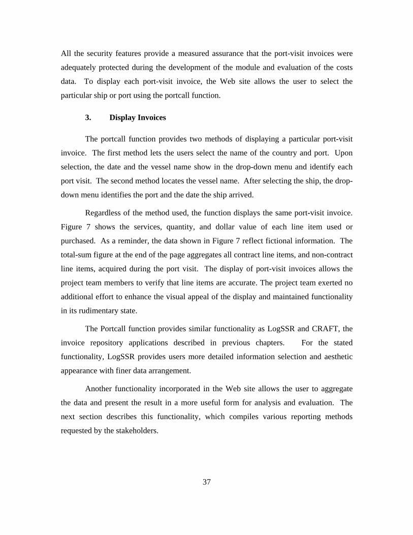
37

All the security features provide a measured assurance that the port-visit invoices were

adequately protected during the development of the module and evaluation of the costs

data. To display each port-visit invoice, the Web site allows the user to select the

particular ship or port using the portcall function.

3. Display Invoices

The portcall function provides two methods of displaying a particular port-visit

invoice. The first method lets the users select the name of the country and port. Upon

selection, the date and the vessel name show in the drop-down menu and identify each

port visit. The second method locates the vessel name. After selecting the ship, the drop-

down menu identifies the port and the date the ship arrived.

Regardless of the method used, the function displays the same port-visit invoice.

Figure 7 shows the services, quantity, and dollar value of each line item used or

purchased. As a reminder, the data shown in Figure 7 reflect fictional information. The

total-sum figure at the end of the page aggregates all contract line items, and non-contract

line items, acquired during the port visit. The display of port-visit invoices allows the

project team members to verify that line items are accurate. The project team exerted no

additional effort to enhance the visual appeal of the display and maintained functionality

in its rudimentary state.

The Portcall function provides similar functionality as LogSSR and CRAFT, the

invoice repository applications described in previous chapters. For the stated

functionality, LogSSR provides users more detailed information selection and aesthetic

appearance with finer data arrangement.

Another functionality incorporated in the Web site allows the user to aggregate

the data and present the result in a more useful form for analysis and evaluation. The

next section describes this functionality, which compiles various reporting methods

requested by the stakeholders.

38

Figure 7. Screenshot of a portcall visit invoice.

4. Generating Reports

The Reports function provides stakeholders the capability to analyze historical

invoices and display a valuable representation of the data. As an example, this Web site

features a report segregating each line item into the appropriate fund code. A user selects

the range that allows the aggregation of all invoices between two specified dates. This

function also lets the user select the sort priority in displaying the report. The first

priority permits sorting by port, which lists the name of countries and is subdivided by

the port names. Each port enumerates the ship types that made port visits and lists the

39

fund codes and aggregated amount of each ship type. The second sorting priority allows

the user to sort by ship type, which shows the aggregated amount spent in each port.

Figure 8 shows the fund-code report selection screen, while Figure 9 displays the

truncated result of the selection.

Figure 8. Screenshot of report selection.

40

Figure 9. Screenshot of fund code report.

While the Reports function provides an exceptional capability for contracting

officers and major claimant stakeholders, the development of LOGCOP provides an

extensive data set in generating reports. By using LOGCOP, a user may intertwine other

reporting categories with the invoice data, which greatly increases the value of the report.

In evaluating the module's functionality, the bread-and-butter of the Web site pertains to

the forecast capability that provides an estimate of future port-visit cost.

41

5. Forecasting

The Estimate function assists the user in determining the future cost of a port

visit. As Figure 10 reflects, the user selects the name of the port, the type of vessel

making the portcall, whether the vessel will be in port or anchored, and the number of

days during the port visit. After selecting the parameters, the module displays the sub-

CLIN types used by other vessels of the same type and the cost estimate of each sub-

CLIN type. Figure 11 shows the estimate. Some sub-CLIN types should not be included

in the estimate, such as CHT removal at anchorage when the user anticipates pulling into

port. The user may opt to exclude sub-CLIN types for services not applicable for the

estimate.

Figure 10. Screenshot of forecasting parameters.

42

Figure 11. Screenshot of a port-visit cost estimate.

The module generates two types of estimates, namely, t-statistics (Keller, 2009,

p. 382) and exponential smoothing (Balakrishan, Render, & Stair, 2007, p. 527). The t-

statistics consists of the estimate's lower boundary, the adjusted average of the sub-CLIN

type costs, and the higher boundary of the estimate. The lower and higher boundaries

reflect the statistical probability, at 95% confidence level, that the actual cost would be

43

between these two numbers. The second forecasting method, called exponential

smoothing, represents a type of time-series or moving average approach that requires a

constant, also called alpha (), to weigh the recent data or past period more than the

other. To determine the optimal constant, the module uses a heuristic algorithm that runs

through several iterations in comparing the mean absolute percentage of error (MAPE) of

alphas, between 0.01 and 1.00, until the algorithm produces the ideal alpha.

The forecast accuracy depends on the error percentage between the actual and the

estimated cost. Accuracy increases as the error percentage decreases. Subsequently, five

scenarios also affect the accuracy of the estimate. The list below states the condition of

each scenario:

F. SAME VESSEL TYPE, SAME PORT, SAME COUNTRY

This scenario states that invoices exist in the database for a similar vessel type

that pulled into the same port. For example, if DDG19 and DDG20 visited Port Maroon,

at Country Zulu in 2007, then DDG21 could forecast an upcoming visit to Port Orange in

2008 by using the invoice data collected from prior DDG visits.

G. SAME VESSEL CLASS, SAME PORT, SAME COUNTRY

This scenario states that no invoices exist for a similar vessel type. However,

invoices for the same vessel class are available in the database for the same port. For

example, the Navy classifies DDGs and CGs as Class 2 vessels. DDG19, DDG20, and

DDG21 visited Port Maroon, but no CG ever pulled into this port. Using this scenario,

CG32 could forecast the ship’s upcoming visit by using the same ship class invoices from

the three DDGs.

H. NOT THE SAME VESSEL TYPE/CLASS, SAME PORT, SAME COUNTRY

Port-visit invoices exist for other vessel types and class only. Using the prior

example, three DDGs and one CG visited Port Maroon. The next ship scheduled to visit

is an LPD, Class 3 ship. Under this scenario, the LPD predicts the port-visit costs for

Port Maroon by using invoices for Class 2 ships.

44

I. NOT THE SAME VESSEL TYPE/CLASS, NOT THE SAME PORT, SAME COUNTRY

Only invoices from other ports of the same country are available for computation.

Continuing with the example, assume that in addition to Port Maroon, Country Zulu has

another port called Port Ruby. No ships have ever pulled into Port Ruby before, but

DDG22 is set to visit the port. In this scenario, DDG22 uses Port Maroon invoices to

produce an estimate of the port-visit costs for Port Ruby.

J. NOT THE SAME COUNTRY; ONLY INVOICES FROM OTHER COUNTRIES ARE AVAILABLE

Assume that Country Yankee borders Country Zulu. No ships have ever pulled

into any Country Yankee port before. Any ship pulling into port, using algorithms for

this scenario, could forecast the port-visit costs using invoices in Country Zulu.

The project team used forecasting algorithms only suitable for the first scenario.

As the level of scenario steps up, expect the level of algorithm sophistication and error

rate, the percentage between the actual costs and predicted costs, to increase as well. The

next chapter describes, in detail, the forecasting methodology used and explains the steps

applied in implementing the algorithms for the first scenario.

45

V. FORECASTING METHODOLOGY

The SPFCM forecasting functionality consists of two estimation methods, namely

t-statistic and exponential smoothing. This chapter describes each method and the

algorithms used to compute the estimated port-visit costs. In addition to describing the

methods and algorithms, this chapter also shows the pseudo-code, as applied in the

forecasting functionality.

A. CONFIDENCE INTERVAL ESTIMATOR

T-statistic, as defined by mathematician William S. Gosset, specifies that both

population mean and population standard deviation are unknown. The sample standard

deviation (s) takes the place of the unknown population standard deviation in the formula.

The Confidence Interval Estimator of each sub-CLIN type reflects the formula below to

include the sample mean ( x ), critical value (t/2), and sample size (n).

1. Select Parameters

As shown in Figure 10, the user must specify four parameters to execute the

forecasting functionality. The user must indicate the type of ship to use and the port to

visit in generating the cost estimate. In addition, the user must also indicate the number

of days in port or at anchorage, including the arrival and departure days.

2. Get Historical Data

The module employs the parametric values to retrieve the historical information

from the database. First, the module creates an array to store invoice headers information

such as the number of days in port, ship type and class, and date of arrival. After storing

46

the invoice headers, the module creates a second array to store invoice items such as sub-

CLIN type identification key, unit of quantity, unit price, and adjusted price per day. The

module also creates a third array to store elements of the CLINs and sub-CLINs for each

sub-CLIN type. To refresh the understanding of CLIN elements, Figure 5 shows the

relationship of CLINs to sub-CLIN types. Lastly, the module creates keys in the sub-

CLIN type array for sum, average, sample size, variation, standard deviation, and

confidence level of each type.

3. Critical Values of Student t-distribution ( /2t )

The module generates a two-tail test distribution array at 95% confidence level.

The array key represents the degree of freedom while the value equates to the t-value.

Figure 12, referring to keys and values, reflects the .025t critical values shown in Kellers’

book, Appendix B, Table 4.

Figure 12. .025t Critical values (95% confidence level).

4. Adjust Invoice Item per Day Quantity

Port visits generally vary from one to seven days. Before averaging the sub-CLIN

type or invoice items of all applicable invoices, the total quantity should be adjusted to

47

reflect the daily charge for each item on each invoice. The adjustment allows the module

to store the variation of a sub-CLIN type in daily quantities rather than managing the total

quantity per visit. The module adjusts the quantity depending on the unit of issue and

type. One-time charges and charges incurred per visit instead of per day, such as the

first-day management fee, per job order, each quantity, and per load, require no

adjustment. The module reduces a day from the denominator for daily charges incurred

after the arrival date or prior to the departure date, such as managerial fees for subsequent

days. Figure 13 shows the pseudo-code for the adjustment method.

Figure 13. “Adjust invoice item per day quantity” pseudo-code.

5. Get the Sub-CLIN Type Average ( x )

Since unit prices may vary from one invoice to another, each invoice item stores

the adjusted daily price by multiplying the adjusted per day quantity with the item's unit

price. The module extracts the sum of all adjusted daily prices with the same sub-CLIN

type. The module also computes the sample size of all invoices with charges incurred for

48

the particular sub-CLIN type. A computational representation for sub-CLIN type

(XX44AB-services) would reflect the formula below followed by the pseudo-code

(Figure 14).

Figure 14. Sub-CLIN type average pseudo-code.

49

6. Get the Variance and Standard Deviation ( 2 &s s )

Using the invoice item array, the module retrieves each invoice item’s actual per

day price to compute for the sub-CLIN type variance. The computational representation

of the variance and standard deviation of the sub-CLIN type XX44AB-services reflects:

Figure 15 shows the pseudo-code for getting the sub-CLIN type variance and

standard deviation.

Figure 15. Standard deviation pseudo-code.

50

7. Get the Sub-CLIN Type Confidence Interval ( /2

st

n )

To produce the lower and upper boundaries of the estimate for each sub-CLIN

type, the module computes for the confidence interval using the critical value from the t-

distribution table, the standard deviation, and the sample size of the sub-CLIN type.

Figure 16 reflects the pseudo-code to generate the confidence interval and to compute the

lower and upper boundaries.

Figure 16. Confidence level pseudo-code.

The t-statistic estimate in this module differs from the cumulative average used in

CRAFT. The module breaks down the computation to the sub-CLIN type level, instead

of averaging the total cost of invoices, to accurately capture the charges or fees outside

the normal distribution of the sub-CLIN type cost. The module provides the user a 95%

chance, based on the historical data, that the sub-CLIN type costs will range between the

lower and upper boundaries of the estimate. In measuring the error rate, the module

computes the percentage of error between the estimate and actual cost of the sub-CLIN

type. A close distance between the actual cost and estimate denotes a low percentage of

error.

51

In addition to the confidence interval estimator, the module also validates the

result using another forecasting method called exponential smoothing. The next section

describes the methodology used to produce the forecasted costs using this particular time-

series model.

B. EXPONENTIAL SMOOTHING

Balakrishnan, Render, and Stair (2007) classify exponential smoothing as a type

of moving averages model that provides a stable forecast by leveling sudden fluctuations

in the costs patterns. The model also applies a smoothing constant, called , in addition

to comparing the previous forecasts for port-visit costs with the actual costs. The

smoothing constant reflects a weighted value from 0 to 1, inclusively, that allows more

emphasis or weight to recent periods (when is closer to 1) instead of past periods (when

is closer to 0). For SPFCM purposes, the module uses 0.01 as the lowest weighted

value. To find the optimum value between 0.01 and 1, the module iterates through all

the invoices in computing the lowest Mean Absolute Percent Error (MAPE). The that

corresponds to the lowest MAPE represents the value used as the smoothing constant in

the formula. The formulas below show the exponential smoothing computation to

include the MAPE computation:

52

1. Do Exponential Smoothing (Forecast[t+1])

The module retrieves the adjusted per day price stored in the sub-CLIN type array

for each key or invoice item. After retrieving the data, the module calls the method that

computes for the optimal smoothing constant. The value returned by the method

represents in the exponential smoothing formula. Figure 17 shows the iterative process

that generates the forecast for the next sub-CLIN type cost, using the exponential

smoothing formula stated above.

53

Figure 17. Exponential smoothing pseudo-code.

2. Find the Optimal Smoothing Constant ()

A linear search method forces the module to iterate 100 times through all invoices

as the module searches for the with the lowest MAPE (0.01 to 1 in increments of 0.01).

Clearly an inefficient way to conduct the search, the method slows down the process

considerably due to the intense demand on the computing system. Therefore, the module

employs another method, called heuristic algorithm, which allows a much faster way of

searching for the lowest MAPE value. Using two initial constants, namely the initial

54

(0.50) and segment (0.25), the module compares the MAPE generated by the two values (

[ + segment] and [ - segment]), and resets the search using the of the lower value

MAPE and dividing the segment by half until the segment reaches 0.01. The

segmentation allows the search to loop for six iterations (i.e., 0.25, 0.125, 0.625, 0.3125,

0.015625, 0.0078125). Figure 18 below shows an example of a heuristic search for the

lowest MAPE where the iterated method shows the that corresponds to the lower

MAPE between a higher and lower .

Figure 18. Example of method iteration in search of the lowest MAPE.

Figure 19 reflects the pseudo-code for the optimal smoothing constant, which

calls on the heuristic method, shown in Figure 20, to generate a MAPE for a specific .

55

Figure 19. Pseudo-code for the generating the smoothing constant.

56

Figure 20. The heuristic method pseudo-code.

The module displays the results of estimates, t-statistics and exponential

smoothing, as reflected in Figure 11 (shown in previous chapter). The t-statistics method

provides a ballpark figure of the actual port-visit costs using the upper and lower limits.

Within the limits, a method provides an estimate based on adjusted per day costs of the

required services. Another method, the exponential smoothing, shows whether the

estimate represents a close forecast by using the trend of past port visits barring any

significant requirements in services or a sudden spike in price or fees (i.e., dockage fee).

The two estimates allow the user to analyze the forecasted costs by comparing the

deviation between the two forecasting models.

57

The next chapter discusses the analysis of forecasted port-visit costs for several

types of ships and ports. The research analysis compares the two models and shows the

module's consistency, or the lack of consistency, in minimizing the error rate as the

historical data increase.

58


59

VI. ANALYSIS

To validate the effectiveness of the forecasting module, the researchers conducted

the analysis using data from actual invoices and estimates generated by the module. The

analysis was conducted using four diverse cases. The cases listed below all operate under

the first scenario, described in Chapter IV, and looked at combinations of ports, ship

types, and classes to compare the actual costs with the forecast and compute the error rate

for each visit:

1. The first case examined the port-visit cost data of two ship types, guided

missile destroyers (DDG) and guided missile cruisers (CG), anchored at

Port Red in country Alpha.

2. The second analysis evaluated two ship types at different ports in the same

country. The two ship types consisted of fleet replenishment oilers (TAO)

at Port Orange and DDGs at Port Yellow, berthed pier side in country

Bravo.

3. The third case involved Class 3 ships, the Landing Transport Dock (LPD),

berthing pier side at Port Green in Country Charlie.

4. The last case involved two different classes of ships, a Class 1-submarine

(SSN) berthed pier-side at port Blue and a Class 4–amphibious assault

ship (LHD) moored pier-side at port Indigo- in Country Delta.

Using 2006 and 2007 port-visit cost invoices as the base or historical data set, the

module forecasted 2008 and, up to a certain extent, 2009 port-visit costs. After generating

the estimates, researchers compared the forecast with the actual 2008 and 2009 invoices.

For each port visit, the researchers produced an estimate based on the ship’s requirements

as indicated in the actual invoice. Subsequent to the comparison, project team members

input the actual invoice data into the database. However, the team members produced

simultaneous estimates in instances when, on the same day, two or more ships entered

port.

60

For example, the module forecasted DDG1 port-visit costs in Port Red, the first

DDG entering port in 2008. After generating the estimate, the researchers entered

DDG1’s actual invoice into the database. The team members repeated the process for all

DDG invoices that visited Port Red, DDG2 to DDG8. Consequently, researchers plotted

the results of the estimates and the actual, total port-visit costs in terms of percentage.

As the historical data increases, the most common observation noticed in the

graphs, in all four cases, reflected a funneling effect of upper and lower boundaries

towards the estimated value. In most cases, the actual total costs remained within these

boundaries. In few cases, the sub-CLIN type costs either significantly exceeded the norm

or an extenuating circumstance occurred during the visit that required an additional sub-

CLIN type. These cases, explained in detail below, deviated from the funneling effect and

showed diverging boundaries instead.

The deviations may have occurred due to a new service fee, with no prior

historical requirement, or a requirement that substantially exceeded the norm. Two other

reasons for deviation may include price changes due to currency exchange rate

fluctuation and scheduled rate differences. Since the analysis lacked pricing-schedule

documentation, which was proprietary, the researchers could not verify or assess these

rate differences. Some reasons for the rate fluctuation may include differences due to

holidays, overtime, season, or experience of the person providing the service.

A. CASE ANALYSIS

1. Two Ship Types Anchored at Port Red, Country Alpha

a. DDG at Anchor

The historical data points, which would be used as the basis of estimates,

consisted of 10 DDG port visits between 2006 and 2007. The estimated data set consisted

of 8 DDG port visits in 2008 and 2009. The port visits ranged from two days to seven

days. Figure 21 depicts the graph of the estimates and actual port-visit costs.

61

The graph illustrates the funneling effect discussed earlier in the chapter,

showing how the module “learns” as the data set increases. All of the actual port-visit

cost data fell within the upper-and lower-limit boundaries. Six out of eight DDG actual

port-visit costs came within 5% to 6% of the estimated costs. DDG 4 and DDG 6 actual

port-visit costs were 10% and 13% below the estimate, respectively. This is a problem

the researchers observed in using percentage as the basis of comparison, since percentage

exaggerates the results even if the differences in actual dollar value were minimal.

Figure 21. Graph of 2008–2009 DDG Actual Port-visit Costs Compared to the Forecasted Costs, Port Red, Country Alpha.

Figure 22 shows the error-rate percentage of the estimate and the

exponential smoothing compared to the actual port-visit cost. The calculated average

percentage error rate of the estimate and exponential smoothing were both 6%.

62

Figure 22. Graph of 2008–2009 DDG Estimate and Exponential Smoothing.

b. CG at Anchor

The data utilized for the basis of the estimates was comprised of four

ships’ invoices during 2006 and 2007. The estimates and actual port-visit costs of the

four CGs that visited port Red in 2008 were also plotted and illustrated in a graph (Figure

23).

Again, the graph showed the funneling and diverging effect on the

boundaries for reasons stated above. The boundaries re-converged as soon as the new

requirement was entered into the database. The exponential smoothing remained close to

the estimated value. However, the actual port-visit costs for CG2, CG3 and CG4 were

below the estimated costs. Several factors may have caused this effect. One factor is the

fluctuation in exchange rates. The U.S. dollar exchange rate might have been higher

compared to Country Alpha’s monetary value during those port visits, decreasing the

total port-visit costs.

63

Figure 23. Graph of 2008–2009 CG Actual Port-visit Costs Compared to the Forecasted Costs, Port Red, Country Alpha.

The graph in Figure 24 shows the error-rate percentage of the estimate and

the exponential smoothing compared to the actual port-visit cost. The calculated

average-percentage error rate of the estimate and exponential smoothing were 11% and

9%, respectively.

Figure 24. Graph of 2008–2009 CG Estimate and Exponential- smoothing Error Rate.

64

2. Two Ship Types at Different Ports in the Same Country

Case 1 illustrated the module predicting the port-visit costs of two different ship

types anchored near a port. Case 2 was conducted to assess if the module could

consistently predict the port-visit costs of ships berthing pier side of a port. The second

analysis evaluated two ship types. The two ship types consisted of fleet replenishment

oilers (TAO) at Port Orange and DDGs at Port Yellow, berthed pier side in Country

Bravo.

a. TAO Visiting Pier Side of Port Orange, Country Bravo

Among the types of ships analyzed, TAO port calls in Port Orange

presented the most extensive collection of information. The historical data points, which

correspond to the basis of estimates, consisted of 42 TAO port visits between 2006 and

2007. Likewise, the estimated data set, represented in Figure 26, also showed an

extensive collection of information. The estimated data set consisted of 26 TAO port

visits in 2008. Both the historical and the forecasted port visits ranged from two days to

several weeks.

The TAO port-visit graph, as shown in Figure 25, reflects the funneling

effect of the t-statistic (estimate, upper and lower boundaries). The distance between the

upper and lower boundaries decreases as the estimated data set increases. The

exponential-smoothing line mostly overlaps the estimate line, especially in later

estimations.

Figure 25. Graph of 2008–2009 TAO Actual Port-visit Costs Compared to the Forecasted Costs, Port Orange, Country Bravo.

65

However, 8 of 26 actual port-visit cost data points exceeded the upper

limit, and one was under the lower limit. The first occurrence of an actual port-visit’s

costs exceeding the upper limit of the estimate happened during TAO9 visit. The invoice

included a dockage fee not incurred prior to TAO9 port visit by any other TAO, between

2006 and 2007. As a result, the estimate provided no forecast for that particular sub-

CLIN type.

Table 2 shows the port visits incurred significantly higher charges on

select services that resulted in actual costs exceeding the forecasted upper-limit boundary.

Even though the historical data reflected data points for the specified sub-CLIN type, the

charges incurred exceeded the calculated norm for TAOs. As stated earlier in the

chapter, the husbanding-contract pricing schedule was not available for research review.

PORT VISIT

TAO10

TAO13

TAO14

TAO16

TAO17

TAO20

TAO24

high cost of potable water and extensive use of forklifts

high cost of potable water

high cost of tug services

high quantity for disposed oily waste, high cost of potable water

CLINs THAT EXCEEDED THE UPPER BOUNDARY

Extensive use of transportation services

high cost of tug services and potable water

high cost of tug services and potable water

Table 2. List of TAO Port Visits that Incurred Actual Costs Beyond Upper Boundary.

The last outlier, TAO26, incurred below-norm charges for transportation

and force protection sub-CLIN types. The ship stayed in port for several weeks and only

requested services under these two CLINs. The dollar value difference between the

estimate and the actual costs was not significant. However, the percentage difference

reflects a 17% error due to the low dollar-value of the adjusted daily average. Figure 26

illustrates the percentage error rate of the estimate and exponential smoothing from the

actual port-visit costs, calculated at 17% and 16%, respectively. Note how the peaks on

the line graph matched the peaks (due to actual costs exceeding the upper boundaries) of

the graph in Figure 25. Without these peaks or outliers, the averaged error rate of the

estimate from the actual port-visit cost was calculated to be 12%.

66

Figure 26. Graph of 2008–2009 TAO Estimate and Exponential- smoothing Error Rate.

b. DDG Visiting Pier Side of Port Yellow, Country Bravo

The graph of the actual port-visit cost and estimates for the fourteen DDGs

that visited Port Yellow pier side is depicted in Figure 27. The graph shows the

funneling and diverging effect of the boundaries discussed earlier. The exponential

smoothing mostly overlaps the estimate line. However, 3 out of 14 actual port-visit costs

exceeded the upper-limit boundary.

Figure 27. Graph of 2008–2009 DDG Actual Port-visit Costs Compared to the Forecasted Costs, Port Yellow, Country Bravo.

67

The first incidence of an actual port-visit’s cost data point exceeding the

upper-limit boundary occurred during DDG1’s port visit. DDG1 ordered a new

requirement, shore power service, which was not required during previous DDG port

visits. The cost of this new requirement was substantial enough to cause the actual cost to

exceed the upper-limit boundary by 55%. The other occurrence of actual port-visit costs

exceeding the boundary happened during the port visits of DDG4 and DDG8. DDG4’s

increased port-visit cost resulted from the additional oil-boom service requirement and a

sudden increase in tug-service cost. Similarly, DDG8’s actual port-visit cost exceeded

the upper limit due to the increased cost of tug services.

The sudden increase in the cost of the tug’s services cannot be explained

by simply looking at the invoice, since the unit of issue for the service is per load.

Without questioning the HSP on why the sudden increase, the researchers can only

conjecture that the increased costs was due to an increased number of tugs used, the

increased number of hours or overtime spent, or to seasonal pricing, depending on the

time the ship- arrived in port (i.e., tides and currents).

Figure 28 shows the percentage error rate of the estimate and exponential

smoothing from the actual port-visit costs. The calculated average-percentage error rate

of the estimate and exponential smoothing were 18% and 20%, respectively.

Figure 28. Graph of 2008–2009 DDG Estimate and Exponential- smoothing Error Rate.

68

3. A Different Class of Ship Visiting Pierside

The previous two cases analyzed the forecasted and actual costs of DDGs, CGs,

and TAOs at anchor or moored pier side at various ports in two different countries. All

these ships were Class 2 ships. Case 3 differed from the first two cases, since it

examined a Landing Transport Dock (LPD), which is a Class 3 ship, berthing pier side at

Port Green in Country Charlie.

The historical data points consisted of five LPD port visits between 2006 and

2007. The estimated data points consisted of five LPD port visits in 2008 and plotted in a

line graph (Figure 29). The graph shows the same converging and diverging effects of

the boundaries, which were commonly observed in the previous graphs. The exponential

smoothing overlaps the estimated value line towards the last three estimations. Four out

of five actual port-visit costs fell within the upper and lower-limit boundaries of the t-

estimate method. The outlier, LPD2, resulted from the ship’s requisition of two different

types of fuel that previous LPDs have not ordered. LPD2 might have carried U.S. Marine

vehicles during the port visit requiring the ship to purchase that commodity.

Figure 29. Graph of 2008–2009 LPD Actual Port-visit Costs Compared to the Forecasted Costs, Port Green, Country Charlie.

69

The graph in Figure 30 exhibits the percentage error rate of the estimate and

exponential smoothing from the actual port-visit costs. The calculated average error rate



4. Two Different Classes of Ships Visiting Multiple Ports in the Same Country

Case 4 carried its own unique set of applications. The module-forecasted port-

visit costs of various types of ships, whether anchored or moored at different ports and

countries. The previous case analyses utilized the robust historical data of port-visit cost

invoices from 2006 and 2007 as the baseline to estimate the port-visit costs for ships in

2008 and 2009. However, the estimates conducted in this final case only used two

historical data sets to forecast future port-visit costs (i.e., 2008 port-visit costs). What if

ships rarely visit a certain port or country? Can the module still provide a port-visit cost

estimate using minimal historical data? Case 4 was conducted to assess whether the

module will work in this type of situation. For this final case analysis, the researchers

examined two different classes of ships: Class 4-amphibious assault ship (LHD) moored

pier side at port Indigo, and a Class 1-submarine (SSN) berthed pier side at Port Blue, in

Country Delta.

70

a. LHD (Class 4 ship) Moored Pier Side at Port Indigo, Country Delta.

The historical data points consisted of two LHD port visits in 2007. The

estimated data points consisted of two LHD port visits in 2008 and plotted in a line graph

(Figure 31). Graphically, the upper-limit boundaries for LHD1 and LHD2 were 400%

and 600% above the estimate, respectively. This is expected, since the historical data

used as the baseline of the estimate function were minimal (i.e., two port-visit cost

invoices in 2007). However, the actual port-visit costs were within the upper and lower-

limit boundaries of the t-estimate. LHD1’s actual port-visit cost was 200% above the

estimate due to additional force-protection service requirements, forklift and man-lift

services and a huge provisions order. As mentioned earlier, this is the limitation of using

percentages vice actual dollar value.

Figure 31. Graph of the Estimates and Actual Port-visit Costs of LHD Visiting Port Indigo, Country Delta.

Figure 32 shows the percentage error rate of the estimate and exponential

smoothing from the actual port-visit costs. The calculated average-percentage error rate


71


b. SSN (Class 1 Ship) Moored Pier Side at Port Blue, Country Delta

A similar situation applied to the analysis of submarines. There were only

four data sets available, all from SSN port visits during 2007. In this case, the module

predicted the port cost of two submarines using the historical data from two previous

visits. As graphically illustrated in Figure 33, the analysis produced the same result as

that of the LHD. The upper-limit boundaries for SSN1 and SSN2 were 29% and 42%

above the estimate, respectively. The exponential smoothing overlaps the estimated cost.

This is expected, since the historical data used as the baseline of the estimate function

were minimal. However, the actual port-visit costs were within 5% of the forecasted

costs and fell within the upper and lower-limit boundaries of the t-estimate.

72

Figure 33. Graph of the Estimates and Actual Port-visit Costs of SSNs Visiting Port Blue, Country Delta.

The graph in Figure 34 shows the percentage error rate of the estimate and

exponential smoothing from the actual port-visit costs. The calculated average-

percentage error rate of the estimate and the exponential smoothing for the actual port-

visit costs were 2% and 1%, respectively.

Figure 34. Graph of 2008–2009 SSN Estimate and Exponential smoothing Error Rate.

73

B. SYNTHESIS

The cases reflect the differences in error rate and limit confidence between low

and high for both frequency and variability. Low visit frequency denotes less available

historical information for the module to accurately compute the next port-visit costs. The

analysis shows two types of variability. “Price” represents the first variability, while

“requirements” marks the second type. Table 3 shows the number of visits that

determines the frequency. The table also reflects the error-rate percentages of both

forecasting methods and the percentage of visits in which actual costs remained within

the confidence limits (between low and high boundaries). The following breakdown

shows the scale for frequency and variability:

1. Frequency: Low frequency is 0–15 visits, and high frequency is, more

than 16 visits in a three-year period.

2. Price Variability: 90% to 100% of actual costs within the limits denotes

low price variability. Less than 90% within the limits denotes high price

variability.

3. Requirement Variability: Higher than 10% average error rate, for both t-

estimate and exponential smoothing, denotes high requirement variability.

As Table 3 reflects, an increase in price and requirement variability corresponds

to an increase in error rate and a greater expectation that the actual costs will exceed the

confidence level. As stated, visit frequency only affects the accuracy of the forecast and

does not necessary affect the movement of the error rate.

74

CGs‐Port Red in

country Alpha 5 4 11% 9% 100%

Low Visit Frequency, Low Price

Variability, High Requirement

Variability

DDGs‐Port Red

in country Alpha 11 8 6% 6% 100%

High Visit Frequency, Low Price

Variability, Low Requirement

Variability

TAOs‐Port

Orange country

Bravo 42 26 17% 16% 70%

High Visit Frequency, High Price


Variability

LPDs‐Port Green

in Country

Charlie 5 5 35% 27% 81%

Low Visit Frequency, High Price


Variability

LHDs‐Port Indigo

Country Delta 2 2 51% 32% 100%



Variability

SSNs‐Port Indigo

Country Delta 2 2 2% 1% 100%


Variability, Low Requirement

Variability

DDGs‐Port

Yellow country

Bravo 12 14 18% 20%

CASEHistorical

Visits

Forecasted

Visits

Error Rate of

Exponential

Smoothing

Actual Costs

Within

Limits

CommentsError Rate of

t‐estimate

High Visit Frequency, High Price


Variability80%

Table 3. Comparison of Error Rates, Exponential-smoothing vs. Estimate.

Figure 35 presents a different view of the information provided in Table 3. The

three-dimensional representation places the results in the axis. The left portion of the

cube, the price variability arrow, signifies a higher probability that a port visit will exceed

the limits. In all cases, the results with high price variability reflect a lower percentage of

staying within the t-estimate boundaries (i.e., TAO, DDG-Port Yellow, and LPD). The

upper half of the cube, the requirement variability arrow, denotes high error rates. The

results of port visits with high requirement variability reflect high error rates for both

forecasting methods.

The Synthesis Cube shows the position of the forecast in relation to the actual

costs. Expect a high error rate when the actual port-visit costs show high requirement

variability compared to the historical data stored in the repository. Also, expect the

forecast costs to be outside of the t-estimate boundaries when actual prices denote high

price variability compared to the historical data. As stated earlier, visit frequency lacks

75

the correlation with both error rate and confidence indicator. However, visit frequency

allows the user to gauge the reliability of the forecast results.

Figure 35. Synthesis Cube of Port-visit Costs.

C. CHAPTER SUMMARY

This chapter discussed the analysis of four cases, under Scenario I algorithms, to

validate the effectiveness of the forecasting module. The analysis emphasized the

importance of port-visit costs forecasting tools, such as SPCFM, in managing and

evaluating costs. These tools provide stakeholders with detailed estimates based on

historical data. Among the stakeholders, the SUPPOs and decision-makers benefit the

most. From the SUPPO’s perspective, the ability to generate a port-visit cost forecast

allows him to determine the budgetary impact of the port-visit requirements. In addition,

the ability to view costs from previous port visits empowers him to reasonably question

noticeable increases in the unit cost of any item in the HSP invoices prior to departure

76

from port. By the same token, the module equips the decision-makers with tools to

ascertain the viability of sending ships to ports, mindful of mission needs and funding

constraints.

The analysis shows that a standardized CLIN structure increases the accuracy of

the estimate. The analysis also captures, through spikes and dips in the graph, the effects

of incremental and sudden changes in the husbanding services. Changes in port or ship

requirements, with no supporting historical data, decrease the accuracy of the forecast

and increase the error rate of both estimating methods. Similar to other data depository

and estimating tools, inaccurate or misleading data results in unusable forecasts.

The project conclusion chapter summarizes the performance of the forecasting

model, accounts for the quality of data used in the analysis, and describes the impact of

an effective module to users and stakeholders.

77

VII. CONCLUSION

A well-established network-based decision support system can only be effective

with accurate and updated stored information. As an enabler to these systems, a stable

data repository, including reporting and forecasting capabilities, provides a valuable tool

to stakeholders in analyzing requirements and cost trends, assuming that the data

collected reflect a true representation of port-visit cost invoices. In addition, the

forecasting capabilities allow the same stakeholders to plan port visits based on sound

budgetary considerations and assess the requirements of ships assigned before the actual

visits. SPCFM provides stakeholders with these capabilities.

A. SPCFM PERFORMANCE

SPCFM functionalities allow the user to store and display the invoices, generate

different types of reports, and forecast future port-visit costs. Systems currently online,

such as LogSSR and CRAFT, have built-in capabilities to perform the data repository

function. All of these, including LOGCOP, have display and reporting functions.

However, detailed forecasts remain elusive. With the SPCFM, the forecast drills down to

the sub-CLIN type level.

The analysis indicates error rate tolerance may not be the same in every port.

Gundemir, Manalang, Metzger, and Pitel (2007, June) stated that ports with low

requirement variability and high frequency of visits reflect more accurate cost forecasting

(p. 39). The analysis clearly shows that low requirement variability contributes more to

the confidence of t-estimate interval, while high frequency contributes to the reliability of

the exponential smoothing results.

Regardless of variability, the number of invoices stored in the database dictates

the accuracy of the SPCFM. An accurate result allows users to evaluate the error-rate

tolerance of a particular port, using the two forecasting methods embedded in the module.

The researchers believe that data quality reinforces the accuracy of results. The saying

“garbage in, garbage out” holds credence in the discussion of data collection.

78

B. DATA QUALITY

True representation of port-visit invoices stems from correct assignment of costs

to sub-CLIN types, segregation of sub-CLIN types from consolidated CLIN costs,

designation of shared services, and consistency in data entry. Regional husbanding

contracts using standard CLIN structure gain a clear advantage to other husbanding

contracts that use non-standard CLIN structure. In most cases, data from invoices using

standard CLIN structure requires no filtering of line item designation prior to inclusion

into the database.

In cases in which line-item numbers in the invoice differ from the data repository

CLINs, the user might designate an item as NC or assign an unrelated sub-CLIN type to

the item. The data points would skew the forecast results by either showing a spike or

dip in the actual value outside of the t-estimate limits.

In cases in which an item or service does not correspond to a particular sub-CLIN

type, the user might inadvertently add that cost to an existing sub-CLIN type, resulting in

a consolidated CLIN cost. Hence, the electronic image of the invoice would reflect

inaccurate information and distort the aggregate value of the affected sub-CLIN types.

Ships pulling into port at the same time might elect to share transportation or

force-protection costs. By not indicating specific sub-CLIN types of the shared costs, the

module will not be able to distinguish the shared nature of the services. The forecast

would reflect lower-than-expected daily service cost for the ship type and increase the

sub-CLIN type error rate.

Consistency in data entry produces more reliable forecasts. Two factors affecting

consistency include a well-structured and easy-to-use application, and user training in the

proper use of the application. A well-structured application identifies discrepancies in

the data-entry process prior to finalizing the invoice submission while a user-friendly

application allows the user to navigate through the functions with relative confidence.

Most importantly, training in the proper use of the application prevents unnecessary

editing and evaluation of an unreliable data set.

79

C. IMPACT TO STAKEHOLDERS

In applying the module to the current environment, SPCFM allows decision-

makers to adapt solutions using more accurate operational planning information with

clear numerical limits. Ships' supply officers may use the module as a make-or-buy tool

in determining the cost advantages of buying services (i.e., potable water, electrical

power) instead of producing it or vice versa. Additionally, other stakeholders, such as

contracting officers may use the module as a monitoring tool to decrease the burden in

auditing invoices and increase contract-performance oversight. Once the standard CLIN

structure has been implemented and entered into the data repository, HSPs may not have

to spend so much time entering invoice data into the system.

Since LogSSR and LOGCOP implements most of the functionalities of the

SPCFM, the module does not need to be used as a fully-implemented application. The

advantage of the SPCFM allows the system administrators to modularize the forecasting

function and embed it into the current system environment. The project's main goal is to

provide the stakeholders with an application that increases the current system capabilities

and a tool to better forecast future port-visit costs. By reducing the error rate to a

tolerable limit and confining the actual port-visit costs within the upper and lower

boundaries of the estimate, the project team members believe the module achieved the

stated goal.

The next chapter discusses recommendations to prevent inclusion of inaccurate

and misleading data into the system. It also includes other recommendations that should

assist the stakeholders in maintaining the integrity of the data. With proper application,

these recommendations will hopefully reduce port-visit costs and increase the ability to

project the feasibility of future port visits.

80


81

VIII. RECOMMENDATIONS

A. STANDARDIZE THE CLIN STRUCTURE OF HUSBANDING SERVICES CONTRACTS

All HSP contracts must adopt the same structure to properly record, accurately

report, and confidently forecast port-visit costs. Regional HSP contracts, such as FISCSI

HSP contracts, apply a standardized CLIN structure. Unfortunately, not all HSP

contracts share the same CLIN structure. The basis of a successful decision-support

system rests on proper classification of identification keys. As stated in an earlier

chapter, additional sub-CLIN types should be assigned to unique port requirements rather

than classifying the requirements as NC or consolidating them with other similar

services.

The lack of standardization clearly has an effect on error rates. Risk of

misclassification greatly increases, especially in ports with a high variability of services.

As a result, the forecasting module generates an estimate outside the t-estimate

boundaries, thereby decreasing the confidence in the forecasts. Effective implementation

of decision support systems in the current system environment means contracting officers

should issue contract modifications to reclassify non-standard CLIN structures. For new

HSP contracts, the use of the standardized structure should be mandated and unused

identification keys should be proactively assigned for all anticipated services, regardless

of utilization frequency. Existing contracts must recognize the new key assignments to

maintain the integrity of the structure.

B. ADD A FORECASTING FUNCTIONALITY INTO EXISTING DATA REPOSITORY APPLICATIONS

Decision-makers, SUPPOs, and contracting officers need a forecasting tool

integrated in the data-repository system. In terms of forecasting the next port-visit costs,

ad hoc and Crystal Ball™ reports, and Excel™ spreadsheets are tedious to generate and

maintain, and they lack the tailored functionality of an integrated forecasting tool,

82

especially for ships.38 Integrated estimating capabilities offer users with distinct

functionality, sensitive to the HSP contract parameters.

The results of descriptive statistics offer users a frame of reference specific to the

data table. However, proper interpretation of the results requires training of all

stakeholders. An integrated forecasting module provides useful information to the user

without the need for interpretation. Using SPCFM as an example, the forecast shows the

user an estimate, a 95% confidence level boundary, a line-item daily cost, and another

forecasting method result to compare the estimate. The display provides straightforward

and easy-to-understand information.

C. ASSIGN A LEAD OFFICE RESPONSIBLE FOR ASSIGNING NEW, UNIQUE CLIN IDENTIFIERS

COMFISCS should assign only one office with the responsibility of safeguarding

the integrity of the standardized CLIN structure to prevent service type duplication and to

maintain the accuracy of the information.

D. USE ONE DATA REPOSITORY FOR ALL HUSBANDING CONTRACTS

The existence of multiple applications for invoice data collection adds to the cost of

system maintenance, software upgrades, and personnel. In using one data repository,

decision-makers reduce costs associated with multiple systems and increase the reliability of

data collected. A single repository application allows the system administrators to quickly

respond to customer inquiries and, most importantly, increase oversight effectiveness.

To keep systems up-to-date, the use of multiple applications demands upgrades

for each system, with allocated overhead costs included in the expense whether

maintenance, personnel, or power usage. Obviously, decreasing the number of repository

systems reduces the funding requirements of applications with similar purposes (i.e.,

collecting and storing HSP invoices).

38 Crystal Ball™ software is an Oracle® product and Excel™ software is a Microsoft® product. These

spreadsheet-based applications are primarily used for optimization, data sorting and filtering, graph generating, modeling, forecasting, and simulation.

83

Data duplication renders the information in multiple non-networked databases

unreliable. Data entry corrections must be done in all databases instead of just one

networked database. As a result, the same invoice may reflect different CLINs, service

quantity, or amount.

Clearly, a networked database increases the effectiveness of contract-performance

oversight. The elimination of redundant applications (not the data back-ups used by the

selected repository) increases data quality and renders the system a reliable source of

contract performance information.

E. TRAIN HSPS IN DATA ENTRY

Current contracts require HSPs to input the invoices into a data repository system.

However, not all are trained in distinguishing the correct service type to use for a

particular service charge. Due to description differences in invoices, HSPs assign NC

codes even when a more suitable sub-CLIN type is available. Although CLIN

standardization addresses some data entry concerns, training HSPs will provides

contracting officers with a baseline of HSP knowledge.

F. INFORM THE FLEET THAT THE TOOL EXISTS

Similar to other user-dependent systems, an application that displays historical

information, generates reports, and predicts the next requirement may only be useful if

users know it exists.

G. AUDIT AND MONITOR THE INFORMATION IN THE DATA REPOSITORY

To consistently ensure data quality and reliability, the contracting officer (KO)

must conduct periodic audits of invoices stored in the repository. The KO may

accomplish this task by randomly selecting a paper copy of an invoice and comparing it

with the information stored in the repository as represented by the invoice’s electronic

image.

84


85

IX. AREAS FOR FURTHER RESEARCH

A. EXPAND THE FORECASTING MODEL TO INCLUDE SCENARIOS II THROUGH V

The project Web-based application chapter (Chapter IV) lists five scenarios in

computing port-visit costs. These scenarios include: same vessel type, same port, same

country; same vessel class, same port, same country; not the same vessel type/class, same

port, same country; not the same vessel type/class, not the same port, same country; and

not the same country, only invoices from adjacent countries are available. This research

project only covers algorithms and analysis addressing cases of the first scenario. As

stated in Chapter IV, the algorithm complexity increases as the scenario steps up. An

expanded algorithm base would enhance the capability of the forecasting model to predict

port-visit costs under all conditions.

B. INTEGRATION OF GLOBAL HUSBANDING SERVICES WITH NETWORK-CENTRIC LOGISTICS SYSTEMS

Integration of husbanding services management tools into a network-centric

logistics system that allows broad access by husbanding contract stakeholders would

significantly reduce communication, analytical, and coordination problems currently

encountered by supply officers, contracting officers, and contractors. A research paper

focusing on this type of implementation should gauge the feasibility of integration

considering security access issues, accountability, and system maintenance.

86


87

LIST OF REFERENCES

Balakrishan, N., Render, B., & Stair, R.M. (2007). Managerial decision modeling (2nd ed.). Upper Saddle River, NJ: Pearson Education.

Buczkowski, C. (2009, June 27). [Personal communication with researchers].

Burke, C. (2009, January/February). Fleet Supply–Honing the Tools to Make Logistics Work. The Navy Supply Corps Newsletter. Retrieved October 14, 2009, from https://www.navsup.navy.mil/scnewsletter/2009/jan-feb/cover6

General Services Administration, Department of Defense, National Aeronautics and Space Administration. (2005, March). Federal Acquisition Regulation (FAR). Washington, DC: Author. Retrieved May 2, 2009, from http://www.acquistion.gov/far/current/pdf/FAR.pdf

Gundemir, M., Manalang, R., Metzger, P., & Pitel, J. (2007, June). Worldwide Husbanding Process Improvement: Comparative Analysis of Contracting Methodologies. MBA professional report, Naval Postgraduate School, Monterey, CA, retrieved from DTIC online database.

Hall, L. & Adams, K. (2007, November/December). Global Husbanding Contracting, A Strategic Approach to Fleet Logistics. The Navy Supply Corps Newsletter. Retrieved May 5, 2009, from https://www.navsup.navy.mil/site/scnewsletter/2007/nov-dec/highlights4.html

Keller, G. (2009). Statistics for management and economics (8thed.). Mason, OH: South-Western Cengage Learning.

King, J. (2009, January 30). Global husbanding services. Unpublished PowerPoint presentation.

King, J. (2009a, June 9). Logistics Support Services Repository (LOGSSR)NAVSISA-CIO brief. Unpublished PowerPoint presentation.

King, J. (2009b, June 9). [Personal communication with researchers].

King, J. (2009, June 11). [Personal communication with researchers].

Navy Supply Systems Command (NAVSUP).(2009a) Commander, Fleet &Industrial Supply Centers (COMFISCS). Retrieved May 5, 2009, from https://www.nvsup.navy.mil/navsup/ourteam/comfiscs

Navy Supply Systems Command (NAVSUP).(2009b). Fleet & Industrial Supply Center Norfolk (FISCN). Retrieved May 5, 2009, from https://www.nvsup.navy.mil/navsup/ourteam/comfiscs/fiscn

88

Navy Supply Systems Command (NAVSUP).(2009c). Fleet & Industrial Supply Center San Diego (FISCSD). Retrieved May 5, 2009, from https://www.navsup.navy.mil/navsup/ourteam/comfiscs/fiscsd

Navy Supply Systems Command (NAVSUP).(2009d). Fleet & Industrial Supply Center Sigonella (FISCSI). Retrieved May 5, 2009, from https://www.navsup.navy.mil/navsup/ourteam/comfiscs/fiscsi

Navy Supply Systems Command (NAVSUP).(2009e). Fleet & Industrial Supply Center Yokosuka (FISCY). Retrieved May 5, 2009, from https://www.navsup.navy.mil/navsup/ourteam/comfiscs/fiscy

Navy Supply Systems Command (NAVSUP). (2009f).Mediterranean regional husbanding contract Statement of Work (SOW). Retrieved June 4, 2009, from https://www.nvsup.navy.mil/navsup/ourteam/comfiscs

C3F, N4A. (2009, July 24). [Personal communication with researchers].

Surface Warfare Officers School Command.(2009). Logistics requirement. Retrieved June 18, 2009, from http://www.fas.org/man/dod-101/navy/docs/swos/ops/72-10.html

Verrastro, P.J. (1996). Applying commercial practices to husbanding services contract. Master’s thesis, Naval Postgraduate School, Monterey, CA, retrieved from DTIC online database.

89

APPENDIX CASE DATA

CG PERCENTAGE PER VISIT

BASED ON ESTIMATE

Visit Total CG1 CG2 CG3 CG4

Lower Limit ‐0.38 ‐0.40 ‐0.33 ‐0.28

Estimate 0.00 0.00 0.00 0.00

Exp Smooth 0.04 ‐0.04 ‐0.02 ‐0.06

Actual 0.00 ‐0.08 ‐0.14 ‐0.17

Upper Limit 0.39 0.58 0.33 0.28

BASED ON EXP SMOOTHING


Lower Limit ‐0.38 ‐0.40 ‐0.33 ‐0.28

Estimate ‐0.04 0.04 0.02 0.06

Exp Smooth 0.00 0.00 0.00 0.00

Actual ‐0.04 ‐0.04 ‐0.12 ‐0.12

Upper Limit 0.39 0.58 0.33 0.28

BASED ON ACTUAL


Estimate 0.00 0.09 0.16 0.20

Exp Smooth 0.04 0.05 0.14 0.13

90

DDG (PORT RED) PERCENTAGE PER VISIT

BASED ON ESTIMATE

Visit Total DDG1 DDG2 DDG3 DDG4 DDG5 DDG6 DDG7 DDG8

Lower Limit ‐0.29 ‐0.29 ‐0.29 ‐0.17 ‐0.16 ‐0.17 ‐0.14 ‐0.14

Estimate 0.00 0.00 0.00 0.00 0.00 0.00 0.00 0.00

Exp Smooth ‐0.08 ‐0.08 ‐0.08 ‐0.04 ‐0.05 ‐0.05 ‐0.07 ‐0.07

Actual 0.06 0.04 ‐0.03 ‐0.10 0.01 ‐0.13 ‐0.06 ‐0.05

Upper Limit 0.29 0.29 0.29 0.17 0.16 0.17 0.14 0.14



Lower Limit ‐0.29 ‐0.29 ‐0.29 ‐0.17 ‐0.16 ‐0.17 ‐0.14 ‐0.14

Estimate 0.08 0.08 0.08 0.05 0.06 0.06 0.07 0.07

Exp Smooth 0.00 0.00 0.00 0.00 0.00 0.00 0.00 0.00

Actual 0.15 0.12 0.05 ‐0.06 0.07 ‐0.08 0.01 0.02

Upper Limit 0.29 0.29 0.29 0.17 0.16 0.17 0.14 0.14

BASED ON ACTUAL


Estimate 0.05 0.03 0.03 0.11 0.01 0.15 0.06 0.06

Exp Smooth 0.13 0.11 0.05 0.06 0.06 0.09 0.01 0.02

91

TAO PER

CENTA

GE PER

VISIT

BASED ON ESTIM

ATE

Visit Total

TAO1

TAO2

TAO3

TAO4

TAO5

TAO6

TAO7

TAO8

TAO9

TAO10

TAO11

TAO12

TAO13

TAO14

TAO15

TAO16

TAO17

TAO18

TAO19

TAO20

TAO21

TAO22

TAO23

TAO24

TAO25

TAO26

Lower Limit

‐0.32

‐0.28

‐0.32

‐0.32

‐0.22

‐0.24

‐0.17

‐0.28

‐0.23

‐0.16

‐0.19

‐0.22

‐0.19

‐0.19

‐0.19

‐0.24

‐0.22

‐0.17

‐0.19

‐0.18

‐0.20

‐0.22

‐0.19

‐0.19

‐0.16

‐0.13

Estim

ate

0.00

0.00

0.00

0.00

0.00

0.00

0.00

0.00

0.00

0.00

0.00

0.00

0.00

0.00

0.00

0.00

0.00

0.00

0.00

0.00

0.00

0.00

0.00

0.00

0.00

0.00

Exp Sm

ooth

‐0.13

‐0.14

‐0.17

‐0.16

‐0.02

‐0.02

0.04

‐0.12

‐0.18

‐0.14

0.02

‐0.06

‐0.01

0.03

0.06

0.04

0.03

0.10

‐0.01

‐0.01

‐0.05

‐0.04

‐0.02

0.00

0.02

‐0.06

Actual

‐0.08

‐0.07

‐0.15

‐0.23

0.09

0.12

0.17

0.12

1.10

0.23

0.09

0.09

0.58

0.72

0.09

0.42

0.26

0.01

‐0.02

0.26

0.13

‐0.03

‐0.04

0.26

0.07

‐0.29

Uppe

r Lim

it0.65

0.28

0.32

0.54

0.22

0.24

0.17

0.28

0.23

0.16

0.19

0.22

0.19

0.19

0.19

0.27

0.22

0.17

0.19

0.18

0.21

0.25

0.19

0.19

0.16

0.13

BASED ON EXP

SMOOTH

ING

Visit Total

TAO1

TAO2

TAO3

TAO4

TAO5

TAO6

TAO7

TAO8

TAO9

TAO10

TAO11

TAO12

TAO13

TAO14

TAO15

TAO16

TAO17

TAO18

TAO19

TAO20

TAO21

TAO22

TAO23

TAO24

TAO25

TAO26

Lower Limit

‐0.21

‐0.16

‐0.18

‐0.19

‐0.20

‐0.22

‐0.20

‐0.19

‐0.06

‐0.02

‐0.21

‐0.17

‐0.19

‐0.21

‐0.24

‐0.27

‐0.24

‐0.25

‐0.18

‐0.17

‐0.17

‐0.18

‐0.17

‐0.19

‐0.18

‐0.07

Estim

ate

0.15

0.17

0.20

0.19

0.02

0.02

‐0.04

0.13

0.22

0.17

‐0.02

0.07

0.01

‐0.03

‐0.06

‐0.04

‐0.03

‐0.09

0.01

0.01

0.05

0.04

0.02

0.00

‐0.02

0.07

Exp Sm

ooth

0.00

0.00

0.00

0.00

0.00

0.00

0.00

0.00

0.00

0.00

0.00

0.00

0.00

0.00

0.00

0.00

0.00

0.00

0.00

0.00

0.00

0.00

0.00

0.00

0.00

0.00

Actual

0.06

0.08

0.02

‐0.08

0.10

0.14

0.12

0.27

1.56

0.43

0.07

0.16

0.60

0.68

0.03

0.36

0.22

‐0.09

‐0.01

0.27

0.19

0.01

‐0.02

0.26

0.05

‐0.24

Uppe

r Lim

it0.90

0.49

0.59

0.83

0.24

0.26

0.12

0.46

0.50

0.35

0.16

0.31

0.20

0.16

0.12

0.22

0.18

0.06

0.20

0.19

0.27

0.31

0.21

0.19

0.14

0.21

Visit Total

TAO1

TAO2

TAO3

TAO4

TAO5

TAO6

TAO7

TAO8

TAO9

TAO10

TAO11

TAO12

TAO13

TAO14

TAO15

TAO16

TAO17

TAO18

TAO19

TAO20

TAO21

TAO22

TAO23

TAO24

TAO25

TAO26

Estim

ate

0.09

0.08

0.18

0.30

0.08

0.11

0.14

0.10

0.52

0.18

0.09

0.08

0.37

0.42

0.09

0.30

0.21

0.01

0.02

0.20

0.12

0.04

0.04

0.21

0.07

0.40

Exp Sm

ooth

0.06

0.08

0.02

0.09

0.09

0.12

0.11

0.21

0.61

0.30

0.07

0.14

0.37

0.40

0.03

0.26

0.18

0.09

0.01

0.21

0.16

0.01

0.02

0.21

0.05

0.31

BASED ON ACTUAL

93

LPD PERCENTAGE PER VISIT

BASED ON ESTIMATE

Visit LPD1 LPD2 LPD3 LPD4 LPD5

Lower Limit ‐0.72 ‐0.52 ‐0.35 ‐0.36 ‐0.56

Estimate 0.00 0.00 0.00 0.00 0.00

Exp Smooth 1.01 0.56 0.02 ‐0.02 ‐0.23

Actual 2.72 2.33 ‐0.01 ‐0.20 ‐0.09

Upper Limit 3.66 1.87 0.37 0.44 0.68



Lower Limit ‐0.86 ‐0.70 ‐0.36 ‐0.35 ‐0.43

Estimate ‐0.50 ‐0.36 ‐0.02 0.02 0.29

Exp Smooth 0.00 0.00 0.00 0.00 0.00

Actual 0.85 1.13 ‐0.03 ‐0.18 0.17

Upper Limit 1.32 0.84 0.35 0.47 1.17


Estimate 0.73 0.70 0.01 0.24 0.10

Exp Smooth 0.46 0.53 0.03 0.22 0.15

BASED ON ACTUAL

94

LHD PERCENTAGE PER VISIT

BASED ON ESTIMATE

Visit LHD1 LHD2

Lower Limit ‐0.69 ‐0.77

Estimate 0.00 0.00

Exp Smooth 0.09 0.63

Actual 1.96 0.60

Upper Limit 4.22 6.01


Visit LHD1 LHD2


Estimate ‐0.08 ‐0.39


Actual 1.73 ‐0.02


Visit LHD1 LHD2

Estimate 0.66 0.38


BASED ON ACTUAL

95

SSN PERCENTAGE PER VISIT

BASED ON ESTIMATE

Visit SSN1 SSN2


Estimate 0.00 0.00


Actual 0.04 0.01



Visit SSN1 SSN2


Estimate ‐0.03 ‐0.03


Actual 0.01 ‐0.02


Visit SSN1 SSN2

Estimate 0.04 0.01


BASED ON ACTUAL

96


97

INITIAL DISTRIBUTION LIST

1. Defense Technical Information Center Ft. Belvoir, VA

2. Dudley Knox Library Naval Postgraduate School Monterey, CA

3. Acquisition Research Program Naval Postgraduate School Monterey, CA

4. Professor Raymond Franck Naval Postgraduate School Graduate School of Business and Public Policy Monterey, CA

5. Professor Douglas Brinkley Naval Postgraduate School Graduate School of Business and Public Policy Monterey, CA

6. CDR Brett Wagner Naval Postgraduate School Graduate School of Business and Public Policy Monterey, CA

7. NAVSUP HQ Code 02 Mechanicsburg, PA

8. COMFISCS Code 200 San Diego, CA

9. COMTHIRDFLEET San Diego, CA

standard port-visit cost forecasting model for u.s. navy ... · pdf filestandard port-visit...

Documents