stable isotope ratios of tap water in the contiguous...
TRANSCRIPT

Stable isotope ratios of tap water in the contiguous USA
Gabriel J. Bowen1,2, James R. Ehleringer2,3, Lesley A. Chesson2, Erik Stange2*, and
Thure E. Cerling2,3
1Earth and Atmospheric Sciences Department, Purdue University, 550 Stadium Mall Dr.,
West Lafayette, IN 47907, United States of America. E-mail: [email protected],
Telephone: 765-496-9344, Fax: 765-496-1210.
2Biology Department, University of Utah, 257 South 1400 East, Salt Lake City, UT
84112, United States of America. E-mail: [email protected],
[email protected], Telephone: 801-581-8917, 801-581-5558.
3IsoForensics, Inc., 423 Wakara Way, Salt Lake City, UT 84108, United States of
America. E-mail: [email protected], Telephone: 801-581-7623.
*Current address: Department of Biological Sciences, Dartmouth College, Hanover, NH
03755, United States of America. E-mail: [email protected], Telephone: 603-
646-2788.
Stable isotope ratios of USA tap water
1

Understanding links between water consumers and climatological (precipitation) sources
is essential for developing strategies to ensure the long-term sustainability of water
supplies. In pursing this understanding, a need exists for tools to study and monitor
complex human-hydrological systems that involve high levels of spatial connectivity and
supply problems that are regional, rather than local, in nature. Here we report the first
national-level survey of stable isotope ratios in tap water, including spatially and
temporally-explicit samples from a large number of cities and towns across the
contiguous United States. We show that intra-annual ranges of tap water isotope ratios
are relatively small (e.g., < 10‰ for δ
1
2
3
4
5
6
7
8
9
10
11
12
13
14
15
16
17
18
19
20
21
22
2H) at most sites. In contrast, spatial variation in
tap water isotope ratios is very large, spanning ranges of 163‰ for δ2H and 23.6‰ for
δ18O. The spatial distribution of tap water isotope ratios at the national level is similar to
that of stable isotope ratios of precipitation. At the regional level, however, pervasive
differences between tap water and precipitation isotope ratios can be attributed to
hydrological factors in the water source to consumer chain. These patterns highlight the
potential for monitoring of tap water isotope ratios to contribute to the study of regional
water supply stability and provide warning signals for impending water resource changes.
We present the first published maps of predicted tap water isotope ratios for the
contiguous USA, which will be useful in guiding future research on human-hydrological
systems and as a tool for applied forensics and traceability studies.
water cycle, hydrogen isotopes, oxygen isotopes, deuterium excess, GIS, map, spatial
analysis, snowpack
2

Introduction 1
2
3
4
5
6
7
8
9
10
11
12
13
14
15
16
17
18
19
20
21
22
Planning for and maintaining sustainable drinking water resources is a major challenge
for human societies. As human populations grow and exert more powerful and
widespread influence on their environment, this challenge will be multiplied through
factors such as increased demand, heightened potential for contamination, and changes in
the characteristics and distribution (both spatial and temporal) of supplies.
Understanding and managing supplies requires routine monitoring and predictive
modeling of the forces exerted by these factors on hydrological systems. Factors such as
population growth and infrastructure for water diversion have increasingly transformed
local shortfalls in supply into regional water management problems. Thus, there is an
increasing need for research programs that use spatial data to identify and characterize
regional water resource issues that have the potential to severely impact large sectors of
society in the coming decades.
The light stable isotope ratios of water (δ2H, δ18O) are parameters that can be easily and
routinely measured for almost any water sample and which can preserve information on
the climatological source (i.e. the location, time, and phase of precipitation) and post-
precipitation history of water. Environmental water resources, including river, ground,
and lake water, derive their H and O isotopic composition primarily from the meteoric
precipitation that supplies them [Gat, 1981; Kendall and Coplen, 2001; Smith et al.,
2002; Dutton et al., 2005]. Natural or artificial mixing of waters from different sources
and of different ages and overland or subsurface flow will mix and propagate the isotopic
3

“signatures” of source water, preserving an integrated signal of the precipitation sources
contributing to water supplies. Other post-precipitation processes such as evaporation
and chemical interaction with minerals in soils and rock have the potential to modify
stable isotope ratios of water, and can commonly be distinguished through consideration
of coupled δ
1
2
3
4
5
6
7
8
9
10
11
12
13
14
15
16
17
18
19
20
21
22
23
2H/δ18O data. Given the potential wealth of information available and the
relative ease of δ2H and δ18O measurements of water, these parameters have already
featured prominently in climatological and hydrological monitoring networks [Rozanski
et al., 1991; Kendall and Coplen, 2001] and could contribute greatly to future networks
focused on the human/hydrological system.
Here we present results from the first national-scale spatiotemporal survey of stable
isotopes in tap water. The new data show that tap water samples exhibit high levels of
spatially coherent isotope ratio variation that can be related to commonality in patterns of
water source and post-precipitation history for water resources in different parts of the
country. A strong relationship exists between tap water isotope ratios and those of
annually averaged local precipitation (as estimated by geostatistical modeling), but robust
differences between tap water and precipitation isotope ratios also exist in many parts of
the USA. These patterns can be related to regional tendencies in water resource selection
and water history, including patterns likely related to high-altitude dominated sources,
seasonally biased recharge, and evaporative loss from natural or artificial surface
reservoirs. Our data provide the first evidence that large, spatially-distributed isotope
sampling networks offer the potential to identify and characterize the magnitude and
regional relevance of such processes within complex human-hydrological systems. Our
4

1
2
3
4
5
6
7
8
9
10
11
12
13
14
15
16
17
18
19
20
21
22
23
goal is to demonstrate these capabilities in order to promote and guide future network-
based data gathering and spatial analysis efforts that will increase the level of scientific
understanding and security of climatically-sensitive, regionally important water
resources. We synthesize our data as a set of predictive tap-water isotope ratio maps that,
when interpreted with respect for the limitations of the underlying data, should benefit
future water resources research efforts as well as fields such as ecology and forensic
sciences where understanding of large-scale patterns of hydrological isotope ratio
variation is increasingly important.
Methods
Sample acquisition
Tap water samples for spatial characterization of USA tap water isotope ratios were
collected between 12/2002 and 8/2003 through a volunteer network consisting of
professors at academic institutions and water managers. Sample sites were selected to
obtain a relatively complete geographic coverage, particularly with respect to known
variability in precipitation isotope ratios within the USA, and to represent inhabited areas
ranging from large cities to small rural communities. Participants who conducted
sampling were instructed to obtain cold tap water from a local source by running the tap
for ~10 seconds before filling, capping, and sealing (with parafilm) a clean 2-dram vial
(poly-lined cap; [e.g., Clark and Fritz, 1997]). Sample vials were returned to the Stable
Isotope Ratios for Environmental Research (SIRFER) lab at the University of Utah,
where they were prepared for analysis within a few weeks to a few months of receipt.
Samples were stored in a cool, dark environment between the time of receipt and
5

1
2
3
4
5
6
7
8
9
10
11
12
13
14
15
16
17
18
19
20
21
22
23
analysis, and before analysis vials were visually inspected for signs of leakage or
evaporation, including water seepage from around the cap or the presence of large air
bubbles in the sample.
An additional set of samples was collected for characterization of seasonal variations in
tap water isotope ratios through a volunteer network. Individuals in 43 cities and towns
in the United States and southern Canada were chosen to provide samples from one or
more location within their city/town. Sample sites were again chosen to cover known
gradients in natural water isotope ratios in the USA and to include a range of small towns
to large cities in a range of physiological and climatological settings. Volunteers
collected samples from one or more taps (e.g., home tap, office or laboratory tap) once
per month from 1/2005 to 1/2006. These samples were received, stored, and checked for
quality assurance using the same protocols as for the spatial characterization samples.
The overall sampling return rate was 91%, and data from the 47 taps in 38 cities with
returns for more than 8 months during the 13 month period are considered here.
Analytical
Samples were analyzed for their δ2H and δ18O values using either “traditional” (spatial
survey) or “on-line” (seasonal survey) preparation methods, with all sample values
reported using δ notation (where δ = (Rsample/Rstandard -1)*1000, R = 2H/1H or 18O/16O) and
normalized on the VSMOW – VSLAP standard scale. For “traditional” analyses,
hydrogen and oxygen isotope ratios were determined from individual aliquots of the
sample. Hydrogen isotope ratios were determined by analysis of H2 gas produced via the
6

reduction of 2 μl of water on 100 mg of Zn reagent at 500° C [modified from Coleman et
al., 1982]. Oxygen isotope ratio determination was made by analysis of CO
1
2
3
4
5
6
7
8
9
10
11
12
13
14
15
16
17
18
19
20
21
22
23
2 equilibrated
with sample water using the method of Fessenden et al. [2002]. For analysis via the “on-
line” method, a single small (10 μl) aliquot of water was injected onto a column of glassy
carbon held at 1400° C to produce H2 and CO gases. These were separated
chromatographically in a helium carrier gas stream and introduced sequentially into the
ion source of an IRMS (Delta +XL, ThermoFinnigan) for isotope ratio determination.
Samples were analyzed in duplicate, with average precision of 1.5‰ for δ2H and 0.2‰
for δ18O (1 σ) for replicate analyses. All data obtained by either method were normalized
to the VSMOW-SLAP scale through repeated analysis of 2 calibrated laboratory working
standards [Coplen, 1996]. Analyses previously reported by Bowen et al. [2005]
demonstrate that isotope ratio data generated using the 2 different preparation techniques
in the SIRFER lab are comparable across a wide range of values.
Spatial analysis
We analyze the tap water data in the context of maps of mean annual precipitation
isotope ratios created using the method of Bowen and Revenaugh [2003]. The method
involves fitting parameters of a non-linear model including latitude, altitude, and spatial
weighting effects to a database of isotope ratio measurements. The model is then applied
to a geo-referenced grid, using the isotope data and ancillary elevation data, to produce a
prediction surface of precipitation isotope ratios. Data for North America were compiled
from the Global Network for Isotopes in Precipitation (GNIP) database [IAEA/WMO,
2004] and literature sources [Friedman et al., 1992, 2002; Welker, 2000; references in
7
Kendall and Coplen, 2001], giving a total of 78 δ2H data and 84 δ18O data for the
contiguous USA and adjacent areas of Canada and Mexico (see supplementary
information). The precipitation data were reduced to precipitation amount-weighted,
annually averaged values as described previously [Kendall and Coplen, 2001; Bowen and
Wilkinson, 2002; see supplementary information]. The North American data were added
to a global database of precipitation isotope ratios [IAEA/WMO, 2004] and used to create
a global mean-annual map using elevation data from the ETOPO5 digital elevation model
[U. S. National Geophysical Data Center, 1998].
1
2
3
4
5
6
7
8
9
10
11
12
13
14
15
16
17
18
19
20
21
22
23
The predictions used here provide imperfect but relatively accurate estimates of the
regional patterns of precipitation isotope ratio variation across most of the contiguous
United States. For example, based on previous statistical analyses of equivalent maps the
average 2 standard deviation uncertainty for these predictions is approximately 8 and
1.0‰ (δ2H and δ18O, respectively) for sites within the USA [Bowen and Revenaugh,
2003]. One significant exception occurs along the Pacific coast in Northern California
and Oregon, where our database does not include sufficient spatial sampling to document
the strong isotopic gradients known to exist between coastal and inland regions [e.g.,
Ingraham and Taylor, 1991]. As a result, we do present tap water isotope ratio data and
predictions for this part of the USA, but do not focus on interpretation of the tap water
data in the context of mapped precipitation isotope ratio estimates in this region.
Additional analysis of spatial patterns in the tap water isotope data were conducted in
ArcGIS 9.1 (ESRI; Redlands, CA, USA; all calculations conducted using grids in US
8

Contiguous States Albers Equal Area Conic projection). Identification of robust spatial
patterns in the data was accomplished using Morans I (Spatial Statistics Toolbox, ArcGIS
9.1) to quantify spatial autocorrelation. These calculations were conducted using
unstandardized weights derived from squared inverse Euclidean distances between data
points. Additional quantification of spatial coherence and the quality of tap water isotope
ratio predictions made by spatial interpolation was accomplished through ordinary
Kriging of the raw, spatial survey tap water data using the Geostatistical Analyst
extension in ArcGIS 9.1 and cross-validation. For further data analysis and to create
prediction maps of average tap water isotope ratios, differences were calculated between
measured isotope ratios and mapped precipitation isotope ratios at each tap water
collection site. Tap minus precipitation difference surfaces for δ
1
2
3
4
5
6
7
8
9
10
11
12
13
14
15
16
17
18
19
20
21
22
2H, δ18O, and d were
generated by ordinary Kriging. All Kriging of raw data and tap-precipitation data used a
spherical semivariogram with nugget. No strong spatial anisotropy was observed in any
of the data sets or incorporated in any of the interpolations. The δ2H and δ18O prediction
maps were created by summing the interpolated USA precipitation isotope layer for each
element and the corresponding Kriged tap minus precipitation difference layer. The d
map was calculated from the tap water H- and O-isotope prediction maps by the equation
d = δ2H - 8 x δ18O. Cross-validation of the Kriged difference layers using Geostatistical
Analyst was used to estimate prediction errors (root mean square error) for the tap water
δ2H and δ18O maps.
Results
9

1
2
3
4
5
6
7
8
9
10
11
12
13
14
15
16
17
18
19
20
21
22
23
Five hundred and ten tap water samples for spatial characterization were obtained from
496 towns and cities within the contiguous United States (Fig. 1). Samples were obtained
from each of the 48 contiguous States, with few sampling gaps greater than ~100 km in
radius. Notable exceptions include sparse sampling in eastern Oregon, central Nevada,
central Texas, and eastern Montana.
The raw data values measured in this study are embargoed by our funding agency, but are
presented here graphically. Readers are encouraged to contact the authors for guidance in
the use and application of the data. The stable isotope ratios of these samples (Figs. 1, 2)
span a large range of values from -152 to +11‰ (δ2H) and -19.4 to +4.2‰ (δ18O).
Average values for the sample set are -66‰ for δ2H and -8.9‰ for δ18O. For each
element the data distribution is somewhat bimodal, with a dominant mode similar to the
lumped average and a minor mode near -118‰ (δ2H) and -16‰ (δ18O). The tap water
data cluster near the Global Meteoric Water Line (δ2H = δ18O x 8 + 10, Craig [1961])
characterizing average global precipitation, but many samples lie below this line.
Deuterium excess (d, d = δ2H – δ18O x 8) values for the sample set range from -22.2 to
22.4‰, with an average value of 5.5‰.
The spatial distribution of tap water stable isotope ratios is non-random (Fig. 1; Moran’s I
= 0.68 and 0.59, Z = 7.9 and 6.8, p <0.01 for δ2H and δ18O, respectively). The lowest
δ2H and δ18O values (< -110‰ and < -14‰, respectively) occur throughout the northern
Rocky Mountain States (primarily Idaho, Montana, Utah, and Wyoming), and samples
from this region comprise the lower, minor mode of the hydrogen and oxygen isotope
10
ratio distributions shown in Figure 2. The highest δ2H and δ18O values for USA tap
water samples (> 0‰ for each element) represent samples from a relatively restricted
region of north-central Texas and south-central Oklahoma. Other samples with relatively
high values were obtained throughout the Gulf Coast States. The general pattern of
spatial variation for isotope ratios of each element is one of decreasing values from low-
latitude, low-elevation coastal regions towards inland, high-latitude, and mountainous
areas. In contrast to the H and O isotope ratio values, d values for the USA tap water
samples show no clear, overarching spatial pattern in their distribution, and values of d
between 5 and 10‰ occur throughout the contiguous United States. Extreme values of d,
however, appear to be limited to certain regions, with the highest d values (> 16‰) found
in the northeastern USA (e.g., New England) and the lowest (< -10‰) concentrated in
southern California and along the lower Colorado River, along the Missouri River, and in
north-central Texas and south-central Oklahoma.
1
2
3
4
5
6
7
8
9
10
11
12
13
14
15
16
17
18
19
20
21
22
23
Five hundred and sixty-eight water samples were collected and analyzed as a part of the
monthly water survey effort. The spatial density of the monthly water survey sampling
sites is much lower than that of the spatial characterization sampling sites, but the
distribution of these sites still encompasses much of the physiographic and climatological
variation present in the lower 48 States (Table 1). These samples represent cities and
towns in 22 of the contiguous United States and the province of Alberta. Sampling
density was lowest through the Great Plains and the south-central States. Although no
explicit accounting of specific water sources is attempted here, we note that the monthly
tap water samples represent water sources ranging from single-home wells to
11

1
2
3
4
5
6
7
8
9
10
11
12
13
14
15
16
17
18
19
20
21
22
23
municipally-distributed water from small towns (e.g., Durham, NH) through major US
cities (e.g., Houston, TX).
The isotope ratios of tap water from the monthly sample set range from -144 to +4‰ for
δ2H (average = -61‰) and from -18.9‰ to +1.2‰ for δ18O (average = -8.4‰). Annual
average δ2H and δ18O values for the monthly sampling locations (calculated as
unweighted averages of the monthly samples) range from -135 to -4‰ (average = -60‰)
and from -17.3 to -0.5‰ (average = -8.2‰), respectively (Table 1). Tests of the mean
and variance of these distributions suggest that the distribution of monthly survey δ2H
and δ18O values is not statistically different than that of the spatial characterization data
set (F-test for variance, p = 0.49 and 0.51; T-test for means, p = 0.28 and 0.33 for δ2H
and δ18O, respectively). Intra-annual variation in tap water isotope ratios was calculated
as the standard deviation of isotope ratios for the monthly samples, and ranges from 1 to
10‰ for δ2H and from 0.1 to 1.7‰ for δ18O (Fig. 3). The average 1σ value across all
sites is 4‰ and 0.6‰ for δ2H and δ18O, respectively, or ~2.3% of the range of values
measured in the spatial characterization survey for each element. Inter-annual variation
(1σ) in tap water d values ranges from 0.9 to 5.4‰, with an average value of 2.2‰, or
approximately 5% of the total range observed for all tap water samples.
The inter-annual variability of tap water isotope ratios exhibits relatively weak spatial
coherence, although some spatial patterns may be expressed in the data set. Most areas
of the country include some sampling locations that exhibit low (i.e. < 5 and 0.6‰, 1σ,
for δ2H and δ18O, respectively) inter-annual variability. Sample locations with the
12

highest inter-annual variability (e.g., >7‰ for δ2H) occur almost exclusively in the
southwestern United States (California, Nevada) and the northeastern and north-central
USA (e.g., Minnesota, New York, Ohio, northern Virginia). In contrast, sampling
locations in the northwestern, Rocky Mountain, Great Plain, and Gulf Coast States are
almost all characterized by low inter-annual variability < 5 and 0.6‰ (1σ, δ
1
2
3
4
5
6
7
8
9
10
11
12
13
14
15
16
17
18
19
20
21
22
2H and δ18O,
respectively).
Temporal Isotopic Variability of Tap Water and the Fidelity of the Spatial Data
Temporal variability in tap water isotope ratios at the local level can be assessed from
data collected for the monthly water sampling project. This is important because the
timing (i.e. month) of sample collection for the spatial tap water survey sampling was not
prescribed, and as a result it is difficult to say with absolute certainty how representative
these single samples are of the average tap water isotope ratios at the sampling sites. In
general, inter-annual variability of tap water isotope ratios was found to be low relative to
the range of variation across the spatial sample set and relative to the major spatial
patterns discussed below. Although we allow that a single year of sampling is probably
not sufficient to provide a comprehensive picture of seasonal tap water isotope ratio
variability, the seasonal survey data currently available suggest that in more than half of
all cases, a sample taken at a random time during the year will be similar to the annual
average value of tap water to within 4‰ for δ2H and 0.6‰ for δ18O, with values for even
extreme months falling within ~12‰ and 1.8‰ of the average values.
13

1
2
3
4
5
6
7
8
9
10
11
12
13
14
15
16
17
18
19
20
21
22
Sample collection times for the spatial survey were not random, however, with 63% of
samples having been collected during the months of December, 2002, and March, 2003,
and it is possible that the isotope ratio data could reflect biases related to the timing of
collections. Because the analyses presented in this paper focus on regional patterns
supported by data from many sample sites, these biases would be of concern primarily if
the dataset included spatial clusters of data biased due to non-random collecting times.
Analysis of sample collection dates within the spatial sample set, however, indicates that
no significant spatial autocorrelation exists for the date of sample collection (Moran’s I =
-0.0047, Z = -0.031, p >> 0.1). Thus, although it is possible that measured values from
single sites may differ from representative annually averaged values at that location due
to the timing of sample collection, spatial patterns supported by multiple data stations are
likely to be representative due to spatial averaging of collecting biases, a conclusion
further supported by the high spatial coherence of the tap water data.
Discussion: Comparative Analysis of Tap Water and Precipitation Isotope Ratio
Data
As noted above, the tap water data show spatially coherent variability. Cross-validation
of tap water isotope ratio predictions generated by ordinary Kriging of the raw isotope
data, for example, indicates that approximately 87% of δ2H and 83% of δ18O variation
within the data set can be explained in terms of the isotope ratios of tap water from
adjacent sample sites alone. This implies that aspects of water source and history that
vary continuously across space exert a dominant control on tap water isotope ratios, an
14

1
2
3
4
5
6
7
8
9
10
11
12
13
14
15
16
17
18
19
20
21
22
23
observation that is perhaps surprising given the great potential for discrete factors (e.g,
catchment boundaries, artificial diversion) to impact water isotope ratio patterns.
Spatial variation in the isotope ratios of precipitation (Fig. 4) represents a source of
spatially continuous variability that exerts strong influence on the distribution of stable
isotopes in meteoric waters [e.g., Kendall and Coplen, 2001; Dutton et al., 2005]. The
overall patterns of variation in the precipitation maps and the tap water data are similar,
with the lowest values occurring in the high-altitude continental regions of the northern
Rocky Mountain interior, and the highest values in low-latitude and altitude areas of the
south-central to southeastern United States. Across the entire tap water data set, strong
correlation exists between tap water isotope ratios and predicted mean annual
precipitation isotope ratios (Fig. 5), with more that 74% of the variation in each isotope
system correlated with local precipitation isotope ratios. Values of d for tap water are
more poorly correlated with those of precipitation (r2 = 0.14; not shown). Despite the
large number of intervening processes, the dominant control on tap water isotope ratios at
the national level appears to be the H- and O-isotope ratios of climatological water
sources near the location of water use.
Despite the overarching control of spatial precipitation isotope ratio patterns on the δ2H
and δ18O values of tap water, strong and systematic differences exist between the two
data sets. For both elements, the distribution of tap water isotope ratios is significantly
broader than that of estimated precipitation (i.e. the standard deviation of tap water
isotope ratios is 45 - 50% greater than that of precipitation). This can be seen in Figure 5
15

as a tendency for tap water δ2H and δ18O values to be higher than local precipitation
values at sites with relatively high water isotope ratios, and lower than precipitation
values at the more
1
2
3
4
5
6
7
8
9
10
11
12
13
14
15
16
17
18
19
20
21
22
23
2H- and 18O-depleted sites. Visual inspection suggests that the
deviation from a 1:1 relation between tap water and precipitation values is similar for
both elements at low isotope ratios, but that the effect is stronger for δ18O than for δ2H at
high values.
Our data set demonstrates a high degree of spatial coherence in the distribution of
differences between tap water and annual average precipitation isotope ratios (Moran’s I
= 0.40, 0.29, 0.2; Z = 4.7, 3.4, 2.6; p < 0.01, 0.01, 0.01 for δ2H, δ18O, and d, respectively;
Fig. 6), implying that spatially autocorrelated processes dominate post-precipitation
isotopic modification. This spatially coherent variation allows us to create interpolated
representations of the tap - precipitation isotope ratio differences that represent 74, 68,
and 43% of the variability for δ2H, δ18O, and d offsets at the national level (Fig. 6). On
the basis of our Kriged maps we distinguish two contrasting patterns in the tap -
precipitation isotope ratio offsets that, we argue, reflect different dominant post-
precipitation processes affecting water resources in the contiguous USA.
“Light” water regions
Stable hydrogen and oxygen isotope ratios of tap water are much lower than those of
local precipitation across most of the western interior of the USA and along the Colorado,
Missouri, and Ohio River valleys. We believe that the low tap water isotope ratios in
these areas can be attributed to three factors. First, the stable isotope ratios of H and O in
16

precipitation are strongly correlated with altitude [e.g., Poage and Chamberlain, 2001;
Bowen and Wilkinson, 2002], and tap water derived from sources recharged with high-
elevation water could have lower isotope ratios than those characteristic of precipitation
at the site of water use. Second, in regions characterized by temperate, continental
climates, the stable isotope ratios of precipitation exhibit strong seasonality [Rozanski, et
al, 1993] and tap water derived from sources recharged primarily with winter-season
water might have isotope ratios that reflect the relatively low δ
1
2
3
4
5
6
7
8
9
10
11
12
13
14
15
16
17
18
19
20
21
22
23
2H and δ18O values of
winter precipitation. Third, the stable isotope ratios of many pre-Holocene groundwaters,
particularly those recharged during end-Pleistocene deglatiation, are much lower than
those of younger groundwater or precipitation [e.g., Fritz et al., 1974; Fontes et al., 1991;
Grasby et al., 2002; Zuber et al., 2004], and tap water derived from these old
groundwaters may have atypically low δ2H and δ18O values.
It is likely that within the light water regions described here all three factors contribute to
the low stable isotope ratios of tap water, and based on the current data set we do not
attempt to distinguish among the factors. The impact of high-elevation water on water
resources in the western USA, for example, has been documented in datasets of river
water isotope ratios [Kendall and Coplen, 2001; Dutton et al., 2005] and in groundwater
studies [e.g., Manning and Solomon, 2003]. Within this region, elevation and seasonality
factors are commonly linked, and the concentrated release of winter-season water during
spring and summer melting of high-elevation snowpack provides an important
opportunity for recharge of groundwater and surface water reservoirs [Wilson and Guan,
2004]. Evidence for the impact of pre-Holocene recharge on the isotope ratios of
17
groundwater within the region has been provided by Smith et al. [2002] based on regional
datasets of isotope ratios of groundwater and precipitation in the Great Basin. Although
the low tap water isotope ratios defining our light water regions may primarily reflect one
of theses factors, without site-specific hydrological and water management information it
is not possible to demonstrate this using our current dataset representing a static time-
slice of tap water isotope distributions.
1
2
3
4
5
6
7
8
9
10
11
12
13
14
15
16
17
18
19
20
21
22
23
Data from continued stable isotope ratio monitoring, however, could provide clear
warning signals of future supply stability problems related to these hydrological factors,
particularly when analyzed in the context of data on climate and water supply
infrastructure. Sub-networks designed to target water supplies drawing from deep,
shallow, and surface reservoirs could monitor for potential supply changes in each type of
hydrological system. In aquifer-supplied systems consuming old groundwater, stable
isotope monitoring might identify the early stages of changes in aquifer status, for
example depletion of old water stocks and replacement by younger recharge. Perhaps
more important, however, monitoring of active surface- and shallow groundwater-
supplied systems might provide a means of detecting the early impacts of
hydroclimatological change on the regionally important sources and supplies of water.
As longer-term datasets are developed, spatial analysis to determine common trends and
relate them to climatological and hydrological forcing factors may lead to improved
understanding of the water supply impacts of factors such as changes in mountain
snowpack [McCabe et al., 2004; Mote et al., 2005].
18

Low d-excess regions 1
2
3
4
5
6
7
8
9
10
11
12
13
14
15
16
17
18
19
20
21
22
23
Across most of the contiguous United States, tap water d values are dominantly either
similar to or slightly less than those of precipitation and only scattered single sites give
values that are significantly different (Fig. 6c). Throughout much of the Great Plains and
the Great Lakes Region, however, large concentrations of sampling sites are
characterized by tap water d values that are much lower (i.e. > 10‰) than local
precipitation. In some of these areas, most notably the lower Great Plains, tap water
isotope ratios are also much higher than those of precipitation. Post-precipitation
changes in d occur in response to evaporative loss of water, particularly under conditions
of low relative humidity [Gat, 1981]. Evaporation also leads to an increase in the δ2H
and δ18O values of the residual water, and the low d values and, in places, high stable
isotope ratios of tap waters can be taken to indicate that a substantial degree of
evaporation is typical of water stocks consumed in these areas.
Surface reservoirs provide approximately 63% of all USA public-supply water [Hutson et
al., 2004], and monitoring and planning for the stability of these water sources represents
a major challenge for water managers. Evaporative water loss from reservoirs can
significantly impact water storage, and its effects on water resource stability, particularly
under changing climatic conditions, can be difficult to incorporate in reservoir planning
models [Adeloye et al., 1999; Montaseri and Adeloye, 2004]. Network-based stable
isotope data provide a means of monitoring rates of water loss and regional water
resource sensitivity to evaporation. Although the isotopic evidence for evaporation
clearly does not in itself provide a warning signal of water resource sensitivity, data
19
1
2
3
4
5
6
7
8
9
10
11
12
13
14
15
16
17
18
19
20
21
22
23
collected over time and analyzed in combination with information on regional climate
and hydrology could be used to characterize and monitor surface water resource
susceptibility to climate change.
Conclusion: From precipitation to tap - a first map of tap water isotope ratios
Our results demonstrate that the distribution of δ2H and δ18O values of tap water across
the contiguous United States is dominated by several levels of spatially patterned
variability. Although they can not always be directly or uniquely attributed to causal
factors, the patterns can be described in terms of the stable isotope ratios of
climatological water sources and post-precipitation processes affecting surface and
groundwater resources. Continued isotope ratio monitoring of tap water through spatial
networks such as that developed here offers a tool for monitoring the impacts of
climatological and hydrological changes on water resource stability across large regions
of the country.
One unique contribution of our study has been to demonstrate that spatially coherent
patterns in a tap water data set appear to reflect regionally pervasive features of water
supply hydrology. We believe that by combining this type of spatial data analysis with
collection of temporal sequences of samples the power of this approach will be greatly
increased. In order to guide further development of these applications we have generated
predictive maps of the estimated stable H- and O-isotope ratios and deuterium excess of
tap water for the contiguous USA to serve as a baseline for future studies (Fig. 7; see
Methods). The creation of these maps follows the logic presented in our discussion: they
20

incorporate both the national-scale similarity between isotope ratios of precipitation and
tap water as well as regional offsets related to post-precipitation water source history. All
three maps represented most of the observed variability in USA spatial tap water data
(regression of predicted values against observations gives r
1
2
3
4
5
6
7
8
9
10
11
12
13
14
15
16
17
18
19
20
21
22
23
2 = 0.93 for δ2H, 0.90 for
δ18O, and 0.57 for d), and root mean square errors for the map predictions (based on
cross-validation) are 12‰ for δ2H and 1.8‰ for δ18O (not available for d).
The maps of tap water stable isotope ratios provide a tool and template for water
resources research using H- and O-isotope ratios, but are also relevant to a wide and
developing range of applications involving the use of stable isotope ratios for tracing the
source of human-produced products. Recent studies of products ranging from foods [e.g.,
Giménez-Miralles et al., 1999; Bowen et al., 2005] to biological pathogens [Kreuzer-
Martin et al., 2004a, b] have suggested that in many cases the δ2H and δ18O values of
water used in the production of inorganic or organic products influences the H- and O-
isotope ratios of the finished products in a predictable manner. As a result, analysis of
the stable isotope ratios of products may be used to constrain the location of origin of
samples if the spatial distribution of isotope ratios for relevant water sources is known.
The tap water maps presented here will, in many cases, provide more appropriate
estimates of the spatial isotope ratio patterns relevant to understanding the origin of
human-produced products, which may incorporate tap water directly (e.g., many bottled
water products) or indirectly (e.g., through use of tap water in growth media for microbial
cultures or irrigation of plants). The tap water maps are also highly relevant to a related
category of applications in which the H- and O-isotope ratios of human body tissues,
21
1
2
3
4
5
6
7
8
9
10
11
12
13
14
15
16
17
18
19
20
21
22
such as hair, nail, and tooth enamel, may be used to reconstruct the location of residence
and/or travel history of individuals for purposes of archaeological and/or forensic
investigation [Fraser et al., 2006].
Our maps represent a first attempt to depict the isotope ratios of tap water at the national
scale, but do not capture the full dynamics controlling tap water isotope ratio distributions
and should be used in awareness of their limitations. Tap water isotope ratios reflect a
complex interplay of physical, chemical, and social processes, including both spatially
continuous and discontinuous effects. Interpolation techniques, even when combined
with spatial modeling of natural water sources as done here, can not capture the full
complexity of spatial tap water isotope ratio variation. A mechanistic, predictive model
for tap water isotope ratios will require both improved understanding of the stable isotope
ratios of water sources (including rivers, lakes, reservoirs, and naturally- and
anthropogenically-recharged groundwater) and the development of models for the social
and political processes that determine access to and selection of reservoirs as sources of
water for consumption. The continuation of isotope ratio monitoring efforts focusing on
a wide range of natural and human components of the hydrological cycle is therefore
needed. These efforts will provide both an improved basis for stable isotope ratio
mapping in human-hydrological systems and improved spatiotemporal data sets
documenting the status and stability of regional water supplies.
Acknowledgements
22

1
2
3
This study has been supported with funding from the TSWG under Task IS-FO-2029 and
IsoForensics, Inc. We offer our sincere thanks to the countless individuals that have
contributed tap water samples to this project.
23

References List
Adeloye, A. J., et al. (1999), Climate change water resources planning impacts
incorporating reservoir surface net evaporation fluxes: A case study, Int. J. .Water
Resour. Dev., 15, 561-581.
Bowen, G. J., and J. Revenaugh (2003), Interpolating the isotopic composition of modern
meteoric precipitation, Water Resour. Res., 39, 1299, doi:10.129/2003WR002086.
Bowen, G. J., and B. Wilkinson (2002), Spatial distribution of δ18O in meteoric
precipitation, Geology, 30, 315-318.
Bowen, G. J., et al. (2005), Stable hydrogen and oxygen isotope ratios of bottled waters
of the world, Rapid Comm. Mass Spectrom., 19, 3442-3450.
Coleman, M. L., et al. (1982), Reduction of water with zinc for hydrogen isotope
analysis, Anal. Chem., 54, 993-995.
Coplen, T. B. (1996), New guidelines for reporting stable hydrogen, carbon, and oxygen
isotope-ratio data, Goechim. Cosmochim. Acta, 60, 3359-3360.
Clark, I., and P. Fritz (1997), Environmental Isotopes in Hydrogeology, 328 pp., Lewis,
Boca Raton, FL.
Craig, H. (1961), Isotopic variations in meteoric waters, Science, 133, 1702-1703.
Dutton, A., et al. (2005), Spatial distribution and seasonal variation in 18O/16O of modern
precipitation and river water across the conterminous United States, Hydrol.
Process., 19, 4121-4146.
Fessenden, J. E., et al. (2002), Rapid 18O analysis of small water and CO2 samples using a
continuous-flow isotope ratio mass spectrometer, Rapid Comm. Mass Spectrom.,
16, 1257-1260.
24

Fontes, J. C., et al. (1991), Paleorecharge by the Niger River (Mali) Deduced from
Groundwater Geochemistry, Water Resour. Res., 27, 199-214.
Fraser, I., et al. (2006), The role of stable isotopes in human identification: a longitudinal
study into the variability of isotopic signals in human hair and nails, Rapid Comm.
Mass Spectrom., 20, 1109-1116.
Friedman, I., et al. (1992), Stable isotope composition of waters in southeastern
California 1. Modern Precipitation, J. Geophys. Res., 97, 5795-5812.
Friedman, I., et al. (2002), Stable isotope compositions of waters in the Great Basin,
United States 2. Modern precipitation, J. Geophys. Res., 107, -.
Fritz, P., et al. (1974), Stable isotope content of a major prairie aquifer in Central
Manitoba, Canada, in Isotope Techniques in Groundwater Hydrology, Vol. I, pp.
379-398, IAEA, Vienna.
Gat, J. R. (1981), Lakes, in Stable Isotope Hydrology: Deuterium and Oxygen-18 in the
Water Cycle. Technical Report Series No. 210, edited by J. R. Gat and R.
Gonfiantini, pp. 203-221, IAEA, Vienna.
Giménez-Miralles, J. E., et al. (1999), Regional origin assignment of red wines from
Valencia (Spain) by 2H NMR and 13C IRMS stable isotope analysis of
fermentative ethanol, J. Agr. Food Chem., 47, 2645-2652.
Grasby, S., and R. Betcher (2002), Regional hydrogeochemistry of the carbonate rock
aquifer, southern Manitoba, Can. J. Earth Sci., 39, 1053-1063.
Hutson, S. S., et al. (2004), Estimated Use of Water in the United States in 2000, 52 pp,
United States Geological Survey Circular 1268, Reston, VA.
IAEA/WMO (2004), Global network for isotopes in precipitation, the GNIP database.
25

Ingraham, N. L., and B. E. Taylor (1991), Light stable isotope systematics of large-scale
hydrologic regimes in California and Nevada, Water Resour. Res., 27, 77-90.
Kendall, C., and T. B. Coplen (2001), Distribution of oxygen-18 and deuterium in river
waters across the United States, Hydrol. Process., 15, 1363-1393.
Kreuzer-Martin, H. W., et al. (2004a), Stable isotope ratios as a tool in microbial
forensics-part 1. Microbial isotopic composition as a function of growth medium,
J. Forensic Sci., 49, 954-960.
Kreuzer-Martin, H. W., et al. (2004b), Stable isotope ratios as a tool in microbial
forensics-part 2. Isotopic variation among different growth media as a tool for
sourcing origins of bacterial cells or spores, J. Forensic Sci., 49, 961-967.
Manning, A. H., and D. K. Solomon (2003), Using noble gases to investigate mountain-
front recharge, J. Hydrol., 275, 194-207.
McCabe, G. J., et al. (2004), Pacific and Atlantic Ocean influences on multidecadal
drought frequency in the United States, Proc. Natl. Acad. Sci. Unit. States Am.,
101, 4136-4141.
Montaseri, M., and A. J. Adeloye (2004), A graphical rule for volumetric evaporation
loss correction in reservoir capacity-yield-performance planning in Urmia region,
Iran, Water Resour. Manag., 18, 55-74.
Mote, P. W., et al. (2005), Declining mountain snowpack in western North America,
Bull. Am. Meteorol. Soc., 86, 39-49.
Poage, M. A., and C. P. Chamberlain (2001), Empirical relationships between elevation
and the stable isotope composition of precipitation and surface waters:
Considerations for studies of paleoelevation change, Amer. J. Sci., 301, 1-15.
26

Rozanski, K., et al. (1993), Isotopic patterns in modern global precipitation, in Climate
Change in Continental Isotopic Records, edited by P. K. Swart, et al., pp. 1-36,
American Geophysical Union, Washington, D.C.
Smith, G. I., et al. (2002), Stable isotope compositions of waters in the Great Basin,
United States 3. Comparison of groundwaters with modern precipitation, J.
Geophys. Res., 107, 4402, doi:4410.1029/2001JD000567.
U. S. National Geophysical Data Center (1998), ETOPO-5 five minute gridded world
elevation, NGDC, Boulder, Colorado, USA.
Welker, J. M. (2000), Isotopic (δ18O) characteristics of weekly precipitation collected
across the USA: an initial analysis with application to water source studies,
Hydrol. Process., 14, 1449-1464.
Wilson, J. L., and H. Guan (2004), Mountain-block hydrology and mountian-front
recharge, in Groundwater Recharge in a Desert Environment: The Southwestern
United States, edited by F. M. Phillips, et al., pp. 113-137, American Geophysical
Union, Washington, DC.
Zuber, A., et al. (2004), Age and flow pattern of groundwater in a Jurassic limestone
aquifer and related Tertiary sands derived from combined isotope, noble gas and
chemical data, J. Hydrol., 286, 87-112.
27

Figure Captions
Figure 1: Observed isotope ratios for tap water samples in the spatial data set. A: δ2H, B:
δ18O, C: deuterium excess. All values in ‰ relative to the VSMOW standard.
Figure 2: Stable H- and O-isotope ratios for spatial data set tap water samples. A:
Covariation of δ2H and δ18O values. The bold black line represents the Global Meteoric
Water Line (δ2H = δ18O x 8 + 10). B & C: Frequency distributions for the individual
isotope ratios. The large black circles show the mean values for each isotope ratio for the
entire data set.
Figure 3: Seasonal variability of H- and O-isotope ratios at sites sampled in the seasonal
survey. Values shown are 1 standard deviation (in ‰) for all single-month values at each
site.
Figure 4: Interpolated δ2H (A), δ18O (B), and deuterium excess (C) of annually averaged
precipitation across the contiguous United States (see Methods). The location of data
stations within and adjacent to the contiguous USA are shown in A and B. All values in
‰ relative to the VSMOW standard.
Figure 5: Regression relationships between observed tap water isotope ratios and
interpolated precipitation isotope ratios at the sites of tap water collection. In each panel
(A: δ2H, B: δ18O; ‰ relative to VSMOW) the empirical least-squares regression
28

(equation given) is shown as a solid black line and a 1:1 relation is given as a dotted
black line.
Figure 6: Differences between observed tap water isotope ratios (A: δ2H, B: δ18O) or
deuterium excess (C) and interpolated values for annual average precipitation (Fig. 4).
Values for individual data collection sites are given as points, which are color coded by
the size of the difference between tap water and precipitation values. In each case, values
that are close to zero (i.e., within 16‰ for δ2H, 2‰ for δ18O, or 4‰ for d) are grouped
and shown as white symbols. Background color fields show regional patterns of the
difference between tap water and precipitation values interpolated by ordinary Kriging
using a spherical semivariogram (see Methods). All values in ‰ units.
Figure 7: Prediction maps showing estimated isotope ratios (A: δ2H, B: δ18O) and
deuterium excess values (C) for tap water in the contiguous United States. Isotope ratio
maps were generated by summing interpolated precipitation isotope ratio layers (Fig. 4)
and interpolated differences between tap water and precipitation isotope ratios (Fig. 6).
The map of d values equals the difference of the δ2H map and 8 x the δ18O map (see
Methods). All values in ‰ relative to the VSMOW standard.
29
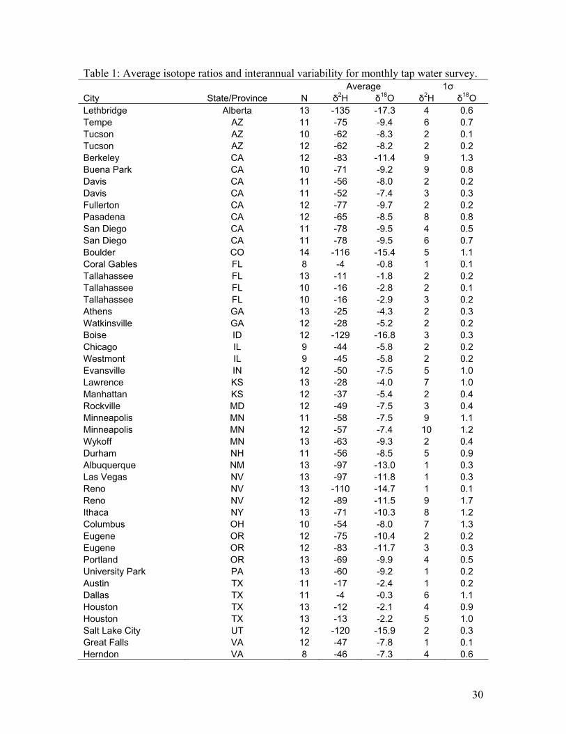
Table 1: Average isotope ratios and interannual variability for monthly tap water survey. Average 1σ City State/Province N δ2H δ18O δ2H δ18O Lethbridge Alberta 13 -135 -17.3 4 0.6 Tempe AZ 11 -75 -9.4 6 0.7 Tucson AZ 10 -62 -8.3 2 0.1 Tucson AZ 12 -62 -8.2 2 0.2 Berkeley CA 12 -83 -11.4 9 1.3 Buena Park CA 10 -71 -9.2 9 0.8 Davis CA 11 -56 -8.0 2 0.2 Davis CA 11 -52 -7.4 3 0.3 Fullerton CA 12 -77 -9.7 2 0.2 Pasadena CA 12 -65 -8.5 8 0.8 San Diego CA 11 -78 -9.5 4 0.5 San Diego CA 11 -78 -9.5 6 0.7 Boulder CO 14 -116 -15.4 5 1.1 Coral Gables FL 8 -4 -0.8 1 0.1 Tallahassee FL 13 -11 -1.8 2 0.2 Tallahassee FL 10 -16 -2.8 2 0.1 Tallahassee FL 10 -16 -2.9 3 0.2 Athens GA 13 -25 -4.3 2 0.3 Watkinsville GA 12 -28 -5.2 2 0.2 Boise ID 12 -129 -16.8 3 0.3 Chicago IL 9 -44 -5.8 2 0.2 Westmont IL 9 -45 -5.8 2 0.2 Evansville IN 12 -50 -7.5 5 1.0 Lawrence KS 13 -28 -4.0 7 1.0 Manhattan KS 12 -37 -5.4 2 0.4 Rockville MD 12 -49 -7.5 3 0.4 Minneapolis MN 11 -58 -7.5 9 1.1 Minneapolis MN 12 -57 -7.4 10 1.2 Wykoff MN 13 -63 -9.3 2 0.4 Durham NH 11 -56 -8.5 5 0.9 Albuquerque NM 13 -97 -13.0 1 0.3 Las Vegas NV 13 -97 -11.8 1 0.3 Reno NV 13 -110 -14.7 1 0.1 Reno NV 12 -89 -11.5 9 1.7 Ithaca NY 13 -71 -10.3 8 1.2 Columbus OH 10 -54 -8.0 7 1.3 Eugene OR 12 -75 -10.4 2 0.2 Eugene OR 12 -83 -11.7 3 0.3 Portland OR 13 -69 -9.9 4 0.5 University Park PA 13 -60 -9.2 1 0.2 Austin TX 11 -17 -2.4 1 0.2 Dallas TX 11 -4 -0.3 6 1.1 Houston TX 13 -12 -2.1 4 0.9 Houston TX 13 -13 -2.2 5 1.0 Salt Lake City UT 12 -120 -15.9 2 0.3 Great Falls VA 12 -47 -7.8 1 0.1 Herndon VA 8 -46 -7.3 4 0.6
30

31

Figure 1: Observed isotope ratios for tap water samples in the spatial data set. A: δ2H, B:
δ18O, C: deuterium excess. All values in ‰ relative to the VSMOW standard.
32

Figure 2: Stable H- and O-isotope ratios for spatial data set tap water samples. A:
Covariation of δ2H and δ18O values. The bold black line represents the Global Meteoric
Water Line (δ2H = δ18O x 8 + 10). B & C: Frequency distributions for the individual
isotope ratios. White stars show the mean values for each isotope ratio for the entire data
set.
33

Figure 3: Seasonal variability of H- and O-isotope ratios at sites sampled in the seasonal
survey. Values shown are 1 standard deviation (in ‰) for all single-month values at each
site.
34

35

Figure 4: Interpolated δ2H (A), δ18O (B), and deuterium excess (C) of annually averaged
precipitation across the contiguous United States (see Methods). The location of data
stations within and adjacent to the contiguous USA are shown in A and B. All values in
‰ relative to the VSMOW standard.
36

Figure 5: Regression relationships between observed tap water isotope ratios and
interpolated precipitation isotope ratios at the sites of tap water collection. In each panel
(A: δ2H, B: δ18O; ‰ relative to VSMOW) the empirical least-squares regression
(equation given) is shown as a solid black line and a 1:1 relation is given as a dotted
black line.
37

38

Figure 6: Differences between observed tap water isotope ratios (A: δ2H, B: δ18O) or
deuterium excess (C) and interpolated values for annual average precipitation (Fig. 4).
Values for individual data collection sites are given as points, which are color coded by
the size of the difference between tap water and precipitation values. In each case, values
that are close to zero (i.e., within 16‰ for δ2H, 2‰ for δ18O, or 4‰ for d) are grouped
and shown as white symbols. Background color fields show regional patterns of the
difference between tap water and precipitation values interpolated by ordinary Kriging
using a spherical semivariogram (see Methods). All values in ‰ units.
39

40
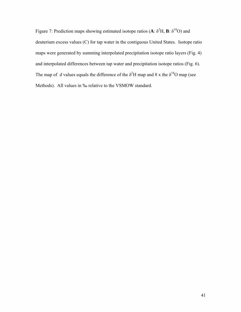
Figure 7: Prediction maps showing estimated isotope ratios (A: δ2H, B: δ18O) and
deuterium excess values (C) for tap water in the contiguous United States. Isotope ratio
maps were generated by summing interpolated precipitation isotope ratio layers (Fig. 4)
and interpolated differences between tap water and precipitation isotope ratios (Fig. 6).
The map of d values equals the difference of the δ2H map and 8 x the δ18O map (see
Methods). All values in ‰ relative to the VSMOW standard.
41