Stable elastic knots with no self-contact

Derek E. MoultonMathematical Institute, University of Oxford, U.K.

Paul GrandgeorgeSorbonne Universite, UPMC Univ Paris 06, CNRS, UMR 7190

Institut Jean Le Rond d’Alembert,F-75005 Paris, France

Sebastien NeukirchSorbonne Universite, UPMC Univ Paris 06, CNRS, UMR 7190

Institut Jean Le Rond d’Alembert,F-75005 Paris, France

March 16, 2018

Abstract

We study an elastic rod bent into an open trefoil knot and clamped at both ends. Thequestion we consider is whether there are stable configurations for which there are no pointsof self-contact. This idea can be fairly easily replicated with a thin strip of paper, but ismore difficult or even impossible with a flexible wire. We search for such configurationswithin the space of three tuning parameters related to the degrees of freedom in a simpleexperiment. Mathematically, we show, both within standard Kirchhoff theory as well withinan elastic strip theory, that stable and contact-free knotted configurations can be found, andwe classify the corresponding parametric regions. Numerical results are complemented withan asymptotic analysis that demonstrates the presence of knots near the doubly-covered ring.In the case of the strip model, quantitative experiments of the region of good knots are alsoprovided to validate the theory.

1 Introduction

Knots are widely familiar structures, from shoelaces and other everyday use to art forms such asCeltic decoration to the many variants employed by sailors. They are often simple to constructand aesthetically appealing, yet remain topologically and mechanically quite complex. They arealso common in biology, appearing in coiled DNA, proteins, and even some species of fish andworms [41, 8].

In polymer studies it has been shown that long enough chains are almost always knotted [37],and DNA being a very long polymer various knots arise in linear or circular molecules. DNAknots arise during replication and transcription of the genetic code and the role of enzymes such

1

Figure 1: Strip of paper knotted in a trefoil with no selft-contact

as topoisomerases is precisely to remove these knots, as the presence of knots has a detrimentaleffect in the cell and can lead to cell death. In viruses, Arsuaga et al have shown that most ofthe molecules are knotted due to compaction in the capside [1]. Biological implications of knotsin DNA are numerous, e.g. the presence of knots in DNA molecules increases their mobility ingel electrophoresis, the compaction of the chain in knotted regions can prevent transcription, andknots can change the speed with which the virus is ejected from the capside [25]. In this lastexample, DNA self-contact has been shown to play an important role in the ejection process.In proteins, for many years knotted structures were not detected, but today over 750 knottedconfigurations are reported in the Protein Data Base; that is more than 1 percent of the entries.These knotted proteins have been shown to catalyse enzymatic reactions [22], play an importantrole in RNA splicing or in the removing of calcium for the cell by membrane proteins [19], andare also present in plant photoreceptors [40]. Simulations of folding and unfolding of proteinsshowed that knotted structures have longer unfolding times than unknotted ones [36]. Knots inproteins also have an important effect on their mechanical stability, making them more resistantto degradation. Moreover, the presence of a knot in a structure brings together active-site residuesand may promote chemical interactions, drive conformational changes, and drive the spontaneousfolding of the structure [18]. The contact interaction in a knotted structure thus appears to be animportant feature of its stability and biological activity, and the question of the presence of suchcontact points or regions in knots therefore emerges.

There are numerous types of questions when studying knots. From a purely mathematicalstandpoint, in topology a knot is an infinitely thin closed loop, and fundamental issues includeknot classification and equivalence of different knot descriptions. A knot in reality obviously differsin that the thickness is finite and the ends are often not closed. This has significant consequencesfor the mechanician, who is typically interested in the strength, equilibrium shape and dynamic

2

behaviour of a knotted filament. Such a description is naturally suited to the theory of elastic rods,but finite thickness in knotted structures by necessity requires consideration of self-contact. Self-contact poses a significant challenge within a rod theory, and it has been approached in differentways computationally [7, 39, 34, 33, 16, 5].

While self-contact is an inherent and inevitable feature of tight knots [30], our aim here isto go the other direction. Namely, we consider the question of whether a knotted filament withzero points of self-contact may be realized physically. In particular, our focus is on the simplelab experiment of an elastic rod bent into a trefoil knot, with the ends held clamped (and forsimplicity, in the absence of gravity). The shape of such a knot in mechanical equilibrium hasbeen considered before [6, 2]. It is characterized by 2 isolated points of self-contact surroundingan interval of self-contact. When twist is increased by rotating one of the clamped ends, thisself-contacting solution becomes unstable and the rod jumps to a nearly planar configuration with4 points of self-contact [6, 5]; see also [20]. The combination of these studies seems to suggestthat such an open trefoil will always have points of self-contact in stable equilibrium. Indeed,such a conjecture has been made [21] in the context of a closed knotted elastic rod and extensivenumerical computations in the contact-free case have only found unstable knotted configurations[11]. However, it is important to note that the ends of the open knot are taken to be perfectlyaligned in the above studies. Experimentally, one can show that if this assumption is removed,then for certain materials and with a little finesse – the right combination of end-rotation andend-displacement – all points of contact can be removed from the open trefoil. We have foundthat for some materials it is difficult if not impossible to achieve, but the result is fairly easilyreproduced with a thin strip of paper or transparency. An example is pictured in Figure 1.

Our objective in this paper is to investigate theoretically such configurations, that is stableequilibrium knots with no points of self-contact. We work within the standard framework of Kirch-hoff equations for inextensible, unshearable elastic rods, and determine stability of an equilibriumstate via linear stability analysis. To mimic the lab experiment, we model an open rod of finitelength clamped with the tangent direction aligned at the ends. The setup for the model is fullyoutlined in Sec 2. Within this setup, there are three tuning parameters: an end-rotation (relatedto the linking number), the end-to-end-displacement, and a transverse end-displacement, i.e. anend-shift. The goal is to characterize the structure of the bifurcation space and the possibilityfor stable contact-free open trefoil knots in terms of these three parameters. To do so, we taketwo distinct approaches. One is to mimic the paper-strip-in-hands experiment by beginning froma configuration in which the rod is in self-contact, with a fixed end-shift and end-displacement,and then rotating the ends until self-contact is lost and the solution moves to a contact-free state.Varying the end-displacement then enables us to construct an ‘island’ in parameter space of ‘goodknots’. This approach forms the subject of Sec 3. The material description of an inextensible rodwith diagonal quadratic bending energy can be characterised by two bending parameters. Sinceour objective is to explore the solution space in terms of the three tuning parameters, in Sec 3 and6 we restrict to a fixed choice of these two material parameters. However, in modelling a ribbon,for instance a strip of paper as in Fig 1, the standard constitutive equations in a Kirchhoff theoryform at best a rough approximation. Hence, in Sec 4 we take an alternative constitutive descrip-tion, and using the elastic strip model described in [9] we find similar qualitative behaviour, buta larger overall region of ‘good knots’. The predictions within the elastic strip theory are tested

3

flip

s = 0

s = L

'/2

'/2

ex

ex

ey

ez

d1(L)

�

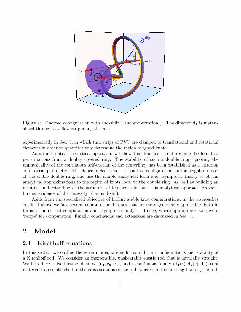
Figure 2: Knotted configuration with end-shift δ and end-rotation ϕ. The director d1 is materi-alized through a yellow strip along the rod.

experimentally in Sec. 5, in which thin strips of PVC are clamped to translational and rotationalelements in order to quantitatively determine the region of ‘good knots’.

As an alternative theoretical approach, we show that knotted structures may be found asperturbations from a doubly covered ring. The stability of such a double ring (ignoring theunphysicality of the continuous self-overlap of the centerline) has been established as a criterionon material parameters [24]. Hence in Sec. 6 we seek knotted configurations in the neighbourhoodof the stable double ring, and use the simple analytical form and asymptotic theory to obtainanalytical approximations to the region of knots local to the double ring. As well as building anintuitive understanding of the structure of knotted solutions, this analytical approach providesfurther evidence of the necessity of an end-shift.

Aside from the specialized objective of finding stable knot configurations, in the approachesoutlined above we face several computational issues that are more generically applicable, both interms of numerical computation and asymptotic analysis. Hence, where appropriate, we give a‘recipe’ for computation. Finally, conclusions and extensions are discussed in Sec. 7.

2 Model

2.1 Kirchhoff equations

In this section we outline the governing equations for equilibrium configurations and stability ofa Kirchhoff rod. We consider an inextensible, unshearable elastic rod that is naturally straight.We introduce a fixed frame, denoted (e1, e2, e3), and a continuous family (d1(s),d2(s),d3(s)) ofmaterial frames attached to the cross-sections of the rod, where s is the arc-length along the rod.

4

The centerline writes r(s, t) = (x, y, z)ei , with 0 ≤ s ≤ L and L the length of the rod. We takethe vector d3(s) to be aligned with the tangent direction, r′(s) = d3(s), where prime denotesdifferentiation with respect to s. The stresses acting at r(s, t) yield a resultant force n(s, t) andresultant moment m(s, t). Note that these quantities can be expressed in either the laboratoryframe or the material frame, i.e. we can write n = (nx, ny, nz)ei = (n1, n2, n3)di

. Assuming norotational inertia, the balance of forces and moments reads:

Balance of forces: n′ + f = ρA r

Balance of moments: m′ + d3 × n = 0,(2.1)

where f(s) is a distributed force acting from outside (gravity, contact, etc.), ρ is the density of thematerial, A the area of the cross-section, and an overdot represents a derivative with respect totime t. The material frames being a family of orthonormal frames, their evolution with arc-lengths is written with the help of a Darboux vector u

d1′ = u× d1 , d2

′ = u× d2 , d3′ = u× d3, (2.2)

which can be interpreted as the strain vector in the rod. We close the set of equations with aconstitutive relation between the moment and the strain

mi =3∑j=1

Bij uj for i = 1, 2, 3 (2.3)

where B is the rigidities matrix. In this paper, we shall restrict to rods with a diagonal rigiditiesmatrix, for which

m = B11 u1 d1 +B22 u2 d2 +B33 u3 d3. (2.4)

Dynamics: equations for components in the material frame

We write (2.1) using components of n and m in the material frames (d1(s),d2(s),d3(s)). Using(2.2), we have for example n′i = (n · di)

′ = (n′ + n × u) · di for i = 1, 2, 3. The dynamics of therod then consists of (2.1), (2.2), as well as r′ = d3, which forms a set of 18 equations for the 18variables (x, y, z, n1, n2, n3, m1, m2, m3, d1x, d1y, d1z, d2x, d2y, d2z, d3x, d3y, d3z), noting thatui = mi/Bii for i = 1, 2, 3 via (2.3). These equations are provided in component form in AppendixA.

Non-dimensionalization

We non-dimensionalize the variables as follows:

nnew =nold L

2

B11

, mnew =mold L

B11

, rnew =roldL,

snew =soldL, unew = uold L, tnew =

toldL2

√B11

ρA.

(2.5)

5

In this way, the material properties of the rod are described by two non-dimensional parameters,

K2 =B22

B11

, K3 =B33

B11

. (2.6)

Here, K2 is the ratio of bending stiffnesses about d2 and d1, while K3 is the ratio of torsionalstiffness to bending stiffness about d1. Unless otherwise stated, we will use the fixed valuesK = K2 = K3 = 3 throughout this paper. This choice is motivated by the result in [24] that thedouble ring is stable if and only if √

K2 − 1

K2

· K3 − 1

K3

≥ 1

2, (2.7)

which in the case K2 = K3 = K reads K ≥ 2. The choice K = 3 ensures that the double ring, andat least some neighbourhood around it, is stable. Though we note that these values are alreadyat the limit of being physically attainable in simple cross-sectional geometries (convex, simplyconnected), as such a rod should satisfy K ≤ 3 for the Poisson ratio to stay above −1/2 [23]. Forinstance, for an elliptical cross-section with major axis a aligned with d1 and minor axis b alignedwith d2, one computes [14]

B11 =Eπab3

12, B22 =

Eπa3b

12, B33 =

Eπa3b3

2(1 + σ)(a2 + b2), (2.8)

where E is the Young’s modulus and σ the Poisson ratio. The choice K2 = K3 = 3 is attained ifa/b =

√3 and σ = −1/2 (auxetic material).

Boundary conditions

In accordance with the experiment shown in Fig 1, we utilize boundary conditions where the rodis clamped at both ends. We take the s = 0 end of the rod to be aligned with the fixed frame atall times:

r(0, t) = (0, 0, 0)T ∀t (2.9a)

d1(0, t) = (1, 0, 0)T ∀t (2.9b)

d2(0, t) = (0, 1, 0)T ∀t (2.9c)

d3(0, t) = (0, 0, 1)T ∀t. (2.9d)

while at the s = 1 end, the rod is held at position (x∗, y∗, z∗) with its tangent aligned with the zdirection

r(1, t) = (x∗, y∗, z∗)T ∀t (2.10a)

d3(1, t) = (0, 0, 1)T ∀t. (2.10b)

The final condition is an imposed end-rotation ϕ

d1(1, t) = (cosϕ, sinϕ, 0)T ∀t (2.11a)

d2(1, t) = (− sinϕ, cosϕ, 0)T ∀t. (2.11b)

6

That is, the material vectors d1 and d2 lie in the x-y plane at s = 1, with d1 making an angleϕ with the x-axis, with ϕ ∈ (0, 2π). In a numerical shooting approach, we thus have 6 equations(2.10a), d3x(1, t) = 0, d3y(1, t) = 0, and arg (d1x(1, t) + ı d1y(1, t)) = ϕ for the 6 unknowns (n1(0),n2(0), n3(0), m1(0), m2(0), m3(0)).

Equilibrium

Setting time derivatives to zero gives an 18D system to solve for equilibrium configurations (seeAppendix A). The boundary conditions read

re(0) = (0, 0, 0)T re(1) = (x∗, y∗, z∗)T (2.12a)

d1e(0) = (1, 0, 0)T d1e(1) = (cosϕ, sinϕ, 0)T (2.12b)

d2e(0) = (0, 1, 0)T d2e(1) = (− sinϕ, cosϕ, 0)T (2.12c)

d3e(0) = (0, 0, 1)T d3e(1) = (0, 0, 1)T . (2.12d)

where we denote equilibrium variables with an e index. As stated in the introduction, we wishto consider the rod’s configurations in terms of the three ‘tuning parameters’ of an end-rotationabout the tangent, an end-displacement, and an end-shift. The end-rotation is the angle ϕ. Sincethe s = 0 end is clamped at the origin with the tangent aligned with the z-direction in the labframe, the end-displacement is determined by the value of ze(1) = z∗, while the end-shift is definedas the magnitude of the distance of the s = 1 end from the point (0, 0, z∗), that is we define

δ =√

(x∗)2 + (y∗)2.

In the case where (x∗, y∗) = 0 it has been shown that solutions are flip-symmetric [12, 17, 27], thatis the 18 functions n1e(s), n2e(s), . . ., d2ze(s), d3ze(s) are either odd or even functions of s − 1/2and the equilibrium shape of the rod is symmetric through a π-rotation about the axis passingthrough point re(1/2) and pointing in the direction d2(1/2). In order to keep the possibility ofhaving flip-symmetric solutions, we choose our transverse end-shift along this flip axis, that is weset

x∗ = −δ cos(ϕ/2)

y∗ = −δ sin(ϕ/2).(2.13)

Note that this does not prove that shifted solutions will remain flip-symmetric, but allows for thepossibility to find such solutions. (A non-flip symmetric solution is shown in Appendix E.)

Stability

To determine stability of an equilibrium solution, we expand the 18 variables as: v(s, t) = ve(s) +ε v(s) eiωt, e.g. n1(s, t) = n1e(s) + ε n1(s) e

iωt, or d3x(s, t) = d3xe(s) + ε d3x(s) eiωt [29, 26]. Inserting

these expansions into the dynamic system, Equations (A.1) in Appendix A, while making useof the equilibrium equations (A.2) and only keeping O(ε) terms would give an 18D eigenvalueproblem for the frequency ω. Following [15], we derive a reduced system if, when writing the

7

perturbations to the directors di(s, t) = die(s) + ε di(s) eiωt, we use the equilibrium directors die

to decompose di, i.e.

di(s) =3∑j=1

αij(s) dje(s) for i = 1, 2, 3. (2.14)

Enforcing orthonormality at order O(ε) yields αij = −αji and αii = 0. The perturbations to thedirectors di are then determined by only three quantities. We introduce the vector

α(s) = α1(s) d1e + α2(s) d2e + α3(s) d3e (2.15)

so that di = α× die. Using this expression and ui(s, t) = uie(s) + ε ui(s) eiωt for i = 1, 2, 3 while

expanding (A.1), we obtain differential equations for the αi(s). The equations for the perturbationsform a system of only 12 equations, provided in full in Appendix A. The condition that the endsof the rod remain clamped and keep their alignment translates to the requirement that each αivanishes at the ends. Thus boundary conditions (2.9), (2.10), (2.11), and (2.12) yield

r(0) = (0, 0, 0)T r(1) = (0, 0, 0)T (2.16a)

α1(0) = 0 α1(1) = 0 (2.16b)

α2(0) = 0 α2(1) = 0 (2.16c)

α3(0) = 0 α3(1) = 0. (2.16d)

Being conservative, such a system only has real-valued ω2 solutions, and an equilibrium solutionis called stable if ω2 > 0 and unstable if ω2 < 0. We then have a linear eigenvalue problemfor ω, with 12 equations and 12 boundary conditions. Note that when numerically solving thiseigenvalue problem, it is convenient to add the normalizing condition

n21(0) + n2

2(0) + n23(0) + m2

1(0) + m22(0) + m2

3(0) = 1 . (2.17)

In a numerical shooting approach, we thus have 7 unknowns (ni(0), mi(0), and ω) and 7 end-conditions (r(1) = 0 and αi(1) = 0).

2.2 ‘Good knots’

We have outlined above the mathematical structure governing the equilibrium shape and stabilityof a clamped elastic rod. As stated, our objective is to seek stable, contact-free, knotted configu-rations as solutions of this system, in terms of the three tuning parameters z∗ (end-displacement),δ (end-shift), and ϕ (end-rotation). To proceed, we must first clarify precisely the configurationswe seek. There are three components:

(1) Knotted. A mathematical knot is always a closed curve, its classification being de-termined by knot invariants. Our interest is the ‘simplest’ knot, the trefoil. Since we areconsidering open configurations with clamped ends, we must clarify the definition of a knotin such a geometry. A natural option, employed here, is to create a closed curve by con-necting the ends through a giant loop at infinity. Whether the closed configuration forms a

8

knot or not depends on how the ends are initially extended beyond the internal portion ofthe rod (the loop at infinity is irrelevant). Here, we make the simple choice of extending therod at both ends, s = 0 and s = 1, along the tangent direction: we lengthen the rod with‘virtual rays’ along the z-axis and connect these rays with a loop at infinity.

In most cases, a formal computation of the extension is unnecessary, and classifying thestructure as knotted or not is a simple matter, e.g. by visual inspection. While performingparameter continuation, the knotted character is monitored by computing the writhe of thecenter line of the rod, as self-crossing will make it jump by two units. More precisely, wecompute the extended polar writheW?

p [31] of the configuration and add to it the total twist

Tw = (1/2π)∫ L0u3(s)ds to obtain a real number that corresponds to the link of the closed

curve mentioned earlier, and we focus on configurations with link between 3 and 4. Theuse of the extended polar writhe measure enables us to detect unknotting due for exampleto the Dirac belt trick, see [31, 32], without having to explicitly consider the rays or loopextending the open curve.

We further introduce the definition of a walled configuration. Such a configuration has0 < z(s) < z?, ∀s ∈ (0, 1), that is the rod entirely lies in the space bounded by two wallsperpendicular to the z-axis. Note that for a walled configuration, the link can be computedusing the classical polar writhe [4], as the Dirac belt trick cannot be performed in thiscase. The walled-knotted configurations are the most clearly identifiable knots visually in aclamped-clamped geometry, and such configurations do not require any concept of tangentextensions. Hence, finding these knots forms a primary focus, though in Section 6 we mustrelax the walled requirement in order to explore the knotted region asymptotically.

(2) Stable. Stability is the most straightforward component. A configuration is deemedstable if all eigenvalues ω satisfy ω2 > 0.

(3) Contact-free. Incorporating self-contact at a finite number of (a priori unknown)points can be achieved within a rod theory [39, 6] by introducing force terms with the formof a delta function centered at an unknown s-location and with unknown magnitude, bothdetermined by appropriate jump conditions across the contact.

Our approach will primarily be to avoid solutions with contact (with one exception - seeSec 3). In general, rather, we shall work within a contact-free rod theory, with no externalforces applied (i.e. f ≡ 0 in (2.1)) and make the assumption that if the centerline of therod does not self intersect, then the configuration corresponds to a contact-free state. Whilemore care would be required to ensure no contact for a rod with given finite cross-sectionalarea, this does provide a necessary and sufficient condition for the existence of a rod withno self-contact, as the cross-sectional area can always in theory be decreased, allowing forappropriate increase in Young’s modulus to maintain the same bending and twist rigidities.

Under the descriptions above, we seek regions of the (z∗-δ-ϕ) parameter space correspondingto ‘good knots’ – walled, knotted, stable, and contact-free configurations. These regions will bebounded by surfaces at which either the configuration becomes unstable (ω2 = 0), does not fit

9

0.2 0.4 0.6 0.8 1.0

j

2 Π

-0.1

0.1

0.2

0.3

0.4

0.5

Tw

A

B

S

W1

W2 X

C

Figure 3: Finding the first good knot. Bifurcation diagram in the (ϕ/2π, Tw) plane for fixedvalues of z∗ = 0.115, δ = 0.05, and K = 3. At point A, the rod is in self-contact (with theray extensions) at two points. Increasing ϕ, experimentally equivalent to rotating the clampedends, the contact points are lost at point B, where the solution jumps to point C. A furtherincrease leads to an interval of good knots, between W1 and W2. A stability boundary is denotedat point S, and a self-crossing boundary beyond which the rod is unknotted is denoted point X.Corresponding rod configurations at points A, B, and X are shown in Figures 4 and 5.

between two walls (mins∈(0,1) z(s) = 0 or maxs∈(0,1) z(s) = z∗), becomes unknotted, or is in self-contact. The latter two typically correspond to the same thing: self-intersection of the centerline,since a walled knot can only change its topology by passing through itself.

3 Results in the Kirchhoff rods case

In this section we compute regions of parameter space corresponding to good knots as numericalsolutions of the 18D system outlined above. A key challenge in this regard is finding a startingpoint, i.e. a choice of parameters for which a desired configuration is known, and that can providebase values for parametric branch tracing. Below, we show that such a starting point can beattained from a known trefoil shape with contact points by varying the end-rotation ϕ in order toremove the contact points. (Later, in Sec 6, an alternative starting point of an unphysical doublering is employed for an analytical approach.) We fix K = 3 in the entire Section.

Removing contacts from a trefoil knot

To start, we fix the parameters z∗ = 0.115, δ = 0.05 and consider a rod held with clamps atboth extremities, with the clamps consisting of long rigid rays aligned with the z-axis. For thesevalues there exists a configuration where the rod contacts the rays at two symmetrical points, one

10

Figure 4: Configurations A and B from Figure 3.

in z < 0 and the other in z > z∗, see configuration A in Figure 4. Such a configuration, wherethe rod is in contact with two obstacles, is obtained by introducing a non-zero shift δ = 0.05on an open trefoil knot with contact [2, 6], following a procedure adapted from [39]. In thisconfiguration A, the circular cross-section of the rod (and of the cylindrical rays) has diameterh = L/200 and the contacts happen at s = 0.17 and s = 0.83; also the end-rotation is ϕ = 0,

twist Tw = (1/2π)∫ L0u3(s)ds ' −0.07, and extended polar writhe W?

p ' 3.07. From here, wegradually increase ϕ (experimentally this would mean rotating the z > z∗ ray around the z-axisin a counter-clockwise way) and the corresponding bifurcation diagram is shown in Figure 3. Asϕ is increased, the intensity of the contact force first increases but then decreases and eventuallyvanishes when ϕ ' 0.768, this is configuration B in Figure 3. From this configuration, contactwith the rigid rays would require a negative adhesive force, hence the rod jumps to a contact-freeknotted configuration, point C in Figure 3. Configuration C is stable and knotted, but not walledas the rod has z(s) < 0 for s ∈ (0.81; 0.85) and z > z∗ = 0.015 for s ∈ (0.15; 0.19). If we furtherincrease the end-rotation from configuration C, we find stable walled knots between point W1

(with ϕW1/(2π) ' 0.774) and point W2 (with ϕW2/(2π) ' 0.82). At point W2 configurations startto exceed the bounding walls again, though remaining knotted and stable. We eventually arriveat point X (with ϕX/(2π) ' 0.96) where the rod self-crosses: configurations with ϕ > ϕX areunknotted.

If from point C we decrease the end-rotation, we see a hysteresis effect: the solution does notjump back to point B but rather follows a branch of knotted, stable, but not-walled solutions.This branch eventually arrives at point S where a pitchfork bifurcation is reached, and stability islost. Two paths of non flip-symmetric solutions depart from the main path, all three paths beingunstable (note that the two paths of non flip-symmetric solutions share the same projection onthe (Tw, ϕ) plane). The main path (with flip-symmetric solutions) eventually crosses the pathof solutions with ray-contact at point B. For these parameters (z∗ = 0.115, δ = 0.05, K = 3)

11

Figure 5: Left: A stable knotted configuration with no self-contact but which does not entirely liebetween walls. It belongs to the path between points W1 and X in Figure 3, with ϕ/(2π) ' 0.88.Right: Configuration X from Figure 3.

0.70 0.75 0.80 0.85 0.90 0.95 1.00

j

2 Π0.0

0.1

0.2

0.3

0.4

0.5

Tw

increasing z*

G

S

W1

W2

X

Figure 6: Left: Bifurcation diagrams for different values of end-shortening. Green regionscorrespond to good knots, blue regions correspond to stable knots that are not between walls,brown regions correspond to unknotted configurations, and red regions correspond to unstableconfigurations. End-displacement values are z∗ = 0.115, 0.150, 0.180, 0.200, 0.215. The parameterδ = 0.05 is fixed. Right: A stable walled knotted configuration with no self-contact, correspondingto point G on the Left.

12

0.70 0.75 0.80 0.85 0.90 0.95 1.00

j

2 Π0.00

0.05

0.10

0.15

0.20

0.25

0.30

z*

S

W1

W2

X

0.5 0.6 0.7 0.8 0.9 1.0

j

2 Π0.00

0.05

0.10

0.15

0.20

0.25

z*

X2

W1

W2

X1

Figure 7: Islands of good knots, plotted in the parameter space of end-displacement z∗ and end-rotation ϕ. The end-shift is fixed at δ = 0.05. Left: The Kirchhoff rod case, where good knotslie inside the region limited by the four curves S, W1, W2, and X. Right: The elastic strip case,where good knots lie inside the region limited by the four curves W1, W2, X1, and X2.

we see that non-flip symmetric knots are all unstable. For other parameter values good non-flipsymmetric knots have been found, though here we will not investigate further non-flip symmetricsolutions.

Island of ‘good knots’

The computations above confirm the theoretical presence of stable, walled, and contact-free knots,indeed showing a continuous interval of such ‘good knots’. We now allow the end-displacementz∗ to vary, while keeping δ = 0.05; the result appears in Figure 6-left, which plots paths of flip-symmetric solutions for different z∗ values. Here, as in Fig 3, green regions represent good knots,blue regions are stable knots that are not between walls, brown regions are unknotted, and redregions are unstable. We see that the interval of end-rotation values for which good knots existis drifting slowly with z∗. We therefore plot in Figure 7-left a connected set of values of ϕ and z∗

for which these stable walled knots exist, i.e. a parametric island of good knots. As illustratedin Fig 7-left, there are three ways for a ‘good’ configuration to lose its properties: (i) it may gounstable (cross the S curve), (ii) it may cross itself and unknot (the X curve), or (iii) it mayextend outside the z = 0 and z = z∗ bounding walls (the Wi curves). Our numerical computationssuggest that this island of good knots shrinks as δ is decreased and vanishes completely for a finitevalue of δ, implying that an end-shift is a requirement for a good knot. Further evidence for thishypothesis is provided by asymptotic calculations for small δ in Section 6.

4 Results in the elastic strip case

One of the assumptions for the validity of Kirchhoff rod theory is that the cross-section is smallcompared to the total length of the structure. Moreover the aspect ratio of the cross-section itselfshould not be too large. For a strip of paper, as in Fig 1, the rectangular cross-section, of width w

13

and thickness h, is flat, h� w, so the assumptions for Kirchhoff theory are not met. In such a case,the system should be modelled using elastic strip equations [13, 35]. Here we follow the approachdeveloped in [10], where elastic strip equations are derived using an energy approach starting fromshell theory. It is shown that in the regime where L � w � h, an elastic strip obeys essentiallythe same equations as an elastic rod, provided the bending and twist constitutive relations arechanged in the following way. We put the width w along the d1 direction and the thickness halong the d2 direction. As a consequence the strip is unbendable around d2 and we thus have

u2(s, t) = 0 ∀ (s, t) (4.1)

even if the bending moment m2 is non-zero. This situation is analogous to the constraint ofinextensibility where the extensional strain in the rod is zero while the axial stress is not. Asecond constraint, coming from differential geometry, is that the inextensibility of the strip surfaceitself implies a link between the bending in the soft direction (u1) and the twist (u3), eventuallymodifying the other two constitutive relations to

m1 = B

(1− u43

u41

)u1 (4.2a)

m3 = 2B

(1 +

u23u21

)u3, (4.2b)

where B = (1/12)h3w/(1 − ν2), with ν the Poisson’s ratio of the material. In the following, weuse B instead of B11 to non-dimensionalize physical quantities, see (2.5).

The dynamics of the strip is then given by system (A.1), complemented by (4.1) and (4.2):a differential-algebraic system that we will try to avoid. In principle (4.2) could be inverted soas to express u1 and u3 as functions of m1 and m3 and one could treat the system (A.1) as wasdone for the rod case: a system of 18 differential equations for the 18 variables (x, y, z, n1, n2, n3,m1, m2, m3, d1x, d1y, d1z, d2x, d2y, d2z, d3x, d3y, d3z). Nevertheless the inversion leads to multipleroots, a matter that complicates the approach. We therefore use an alternative procedure anddifferentiate (4.2) with respect to s in order to write

u′1 =u31

(u21 + u23)3

[u1 (u21 + 3u23)m

′1 + 2u23m

′3

]u′3 =

u21

2 (u21 + u23)3

[(u41 + 3u43)m

′3 + 4u1 u

33m

′1

],

(4.3)

where m′1 and m′3 are replaced using (A.1d), (A.1f), and (4.1). System (A.1), (4.3) then com-prises 20 equations for the 20 variables (x, y, z, n1, n2, n3, m1, m2, m3, d1x, d1y, d1z, d2x, d2y,d2z, d3x, d3y, d3z, u1, u3) with boundary conditions given by (2.9), (2.10), and (2.11), supple-mented with (4.2) evaluated at s = 0. Numerical shooting now involves the 6 unknowns (n1(0),n2(0), n3(0), u1(0), m2(0), u3(0)) and the 6 equations (2.10), d3x(1, t) = 0, d3y(1, t) = 0, andarg (d1x(1, t) + ı d1y(1, t)) = ϕ. If one interprets the non-linear constitutive relation (4.2a) as alinear relation such that the term in parenthesis plays the role of a non-uniform effective bendingrigidity, one sees that the local twist rate u3(s) lowers the rigidity in bending. This effective rigidity

14

0.5 0.6 0.7 0.8 0.9 1.0

j

2 Π0.0

0.1

0.2

0.3

0.4

0.5

Tw

increasing z*

Figure 8: Left: Bifurcation diagram for different values of the end-displacement z∗ in the elasticstrip case. Green regions represent good knots, blue regions stable knots that are not betweenwalls, and brown regions unknotted configurations. End-displacement values are (following thearrow) z∗ = 0.115, 0.150, 0.180, 0.200, 0.215. The parameter δ = 0.05 is fixed. The point on theupper curve corresponds to the configuration shown on the right. Right: A stable walled knottedelastic strip configuration with no self-contact, with z∗ = 0.215 and ϕ/(2π) ' 0.94.

is cancelled at those points along the rod where u3(s) = u1(s) and reversed when |u3(s)| > |u1(s)|.The relation (4.2b) shows that the opposite is true for the twist constitutive relation: the localtwist rate increases the effective twist rigidity.

Island of ‘good knots’ in the elastic strip case

As with the Kirchhoff model, we compute regions of the parameter space corresponding to goodknots in the elastic strip case. In Figure 8, a bifurcation diagram in the (Tw, ϕ) projection isshown for the same values of z∗ and δ as in Figure 6-left. We see that the end-rotation range forwhich knotted but not walled (blue curves) and good knot (green curves) configurations exist islarger in the strip case than in the rod case. Moreover, equilibrium configurations are found downto values ϕ < 0.5, and no pitchfork bifurcation nor non-flip-symmetric solutions are found. Incomparison with the Kirchhoff rod case, we plot in Figure 7-right the island of good knots for thestrip model, i.e. the parameter range (ϕ, z∗) corresponding to good knots, keeping the end-shiftfixed at δ = 0.05. In the 3D parameter space (δ, z∗, ϕ), we have not found any good knots outsidethe region bounded by 0.01 < δ < 0.3, 0.05 < z∗ < 0.45, and 0.02 < 1 − ϕ/(2π) < 0.5, seeFigure 9. Nevertheless, as in the Kirchhoff rod case, we have numerically found stable knottedunwalled configurations as δ → 0, see Section 6 for asymptotic calculations on this matter.

15

Figure 9: In the elastic strip case, regions for good knots (green), unwalled knots (blue), andunkotted configurations (brown) in the 3D space (δ, z∗, ϕ), for δ = 0.01, 0.05, 0.10, 0.15, 0.20,0.25, and 0.30.

5 Experimental validation

We have shown that parameter values exist for stable, contact-free and walled knots, in both theKirchhoff rod and Elastic Strip cases. As highlighted in the introduction, the three parameters ofend-displacement, end-rotation, and end-shift are easily manipulated in an experimental setting.In this section, we perform a quantitative experiment to test and validate the theoretical predic-tions. In particular, we focus experimentally on the elastic strip case. As seen above, the stripmodel predicts a larger region of good knots, thus increasing the chances of finding these configura-tions experimentally. Also, a material fitting the assumptions of the strip model is easily obtained,while the material parameters we have utilised in the Kirchhoff theory (K2 = K3 = 3), thoughphysically possible, are much harder to manufacture (potentially requiring an auxetic material).

Experimental setup

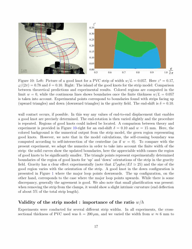
The experimental setup is presented in Figure 10-left. We use strips cut from PVC binding cover,with length L = 26.3 cm, width w ∈ (6, 15) mm, thickness h = 200µm, Young’s modulus E ' 3GPa, density ρ = 1380 kg/m3. At both ends clamps, laser-cut from a 8 mm thick PMMA sheet,bind the strip to rotational Thorlabs elements (enabling precise tuning of ϕ), and these elementsthemselves are mounted on Thorlabs translational elements, one in the z direction for tuningend-displacement z? and one in the transverse x direction, for δ tuning. Translational precision isaround 1 mm, thus the error for z? and δ is around ±0.2 %. For rotation, the imprecision in angleis around 1◦, so the error on the link ϕ is around ±0.3 %. For a given strip, the experimentalprocedure is to fix the end-shift and the end-rotation, and then vary the end-displacement (bysliding one rotational clamp along its translational axis in the z-direction) until self-contact or

16

1 cm

���������

����

����

������

�

�

�

�����

����

���

������

������

0.5 0.6 0.7 0.8 0.9 1.0�

2 Π0.00

0.05

0.10

0.15

0.20

0.25

0.30

0.35z�

Figure 10: Left: Picture of a good knot for a PVC strip of width w/L = 0.057. Here z? = 0.17,ϕ/(2π) = 0.78 and δ = 0.10. Right: The island of the good knots for the strip model: Comparisonbetween theoretical predictions and experimental results. Colored regions are computed in thelimit w = 0, while the continuous lines shows boundaries once the finite thickness w/L = 0.057is taken into account. Experimental points correspond to boundaries found with strips facing up(upward triangles) and down (downward triangles) in the gravity field. The end-shift is δ = 0.10.

wall contact occurs, if possible. In this way any values of end-to-end displacement that enablesa good knot are precisely determined. The end-rotation is then varied slightly and the procedureis repeated. Regions of good knots could indeed be located. A comparison between theory andexperiment is provided in Figure 10-right for an end-shift δ = 0.10 and w = 15 mm. Here, thecolored background is the numerical output from the strip model, the green region representinggood knots. However, we note that in the model calculations, the self-crossing boundary wascomputed according to self-intersection of the centreline (as if w = 0). To compare with thepresent experiment, we adapt the numerics in order to take into account the finite width of thestrip: the solid curves show the updated boundaries, here the appreciable width causes the regionof good knots to be significantly smaller. The triangle points represent experimentally determinedboundaries of the region of good knots for ‘up’ and ‘down’ orientations of the strip in the gravityfield. Gravity has a clear effect experimentally (note that L3ρghw/EI ' 25) and the size of thegood region varies with the orientation of the strip. A good knot in the down configuration ispresented in Figure 1 where the major loop points downwards. The up configuration, on theother hand, corresponds to the case where the major loop points upwards. While there is somediscrepancy, generally the agreement is good. We also note that small plastification was present:when removing the strip from the clamps, it would show a slight intrinsic curvature (end deflectionof about 5% of the total strip length).

Validity of the strip model : importance of the ratio w/h

Experiments were conducted for several different strip widths. In all experiments, the cross-sectional thickness of PVC used was h = 200µm, and we varied the width from w ≈ 6 mm to

17

w ≈ 15 mm, hence the aspect ratio w/h varied from about 30 to 75. The behaviour of the systemwas found to depend on the width w of the strip as follows:

• For w lower than ∼ 6 mm (w/h < 30), the presence of dynamic instabilities was observed,reminiscent of the Kirchhoff rod case: at particular fixed z?, decreasing ϕ slowly would leadto a sudden jump to a new configuration.

• For w larger than ∼ 6 mm (w/h > 30), stability jumps were not observed, though we foundthat the size of the ‘good knot’ island was strongly dependent on w. Moreover, for w . 8mm (w/h = 40), experimental results did not match well with predictions of the elastic stripmodel. Improvement was observed for a wider strip w = 10 mm but only for w & 15 mm didthe comparison between theoretical prediction and experimental results become satisfactory.

This w/h dependence is not included in the elastic strip model, which treats the strip as aplate with no extension, that is u2 is constrained to be zero at all times, an assumption that is metexperimentally for large w/h ratios only. As this ratio becomes smaller, say O(10), the curvatureu2 is no longer infinitely small compared to u1 and u3 and the elastic strip model should then beenriched in order to describe such experimental systems.

6 Unfolding of the doubly covered ring

Figure 11: Beginning at the the doubly-covered ring (middle) and adding a small end-displacement,a small end-rotation and end-shift of opposite sign creates an unknotted helical-type configuration(left), while a small end-rotation and end-shift of equal sign can create a knotted configuration(right).

As an alternative approach to finding regions of parameter space with ‘good knots’, in thissection we take as a starting point the doubly covered ring – this is an unphysical configuration

18

Figure 12: Schematic of configurations of rod centerline for end-displacement 0 < z∗ � 1. Theorigin (which corresponds to zero end-rotation (∆ϕ = 0) and zero end-shift (δ = 0) has 4 pointsof self-contact. Small changes in δ and ∆ϕ can remove the self-contact and divide the quadrantδ > 0,∆ϕ > 0 into 3 regions, separated by two curves with one point of self-contact each. Knottedsolutions exist only in the wedge region (b).

in which the centerline is a circle that traces over itself exactly once and that corresponds toend-rotation ϕ = 2π, end-shift δ = 0, and end-displacement z∗ = 0. The key observation is thatknots can be found emerging from this configuration upon application of a small tuning of theparameters. This idea is easily replicated with a strip of paper: curve a thin strip of paper into adouble circle, such that the ends are in contact, and then shift the ends in the transverse direction.Shifting in one direction creates an unknotted helical-type shape, while passing one end throughthe middle and shifting in the other direction creates a knot, as illustrated in Figure 11. Herewe have included the tangent extensions to the numerically computed configurations, from whichit can be concluded that the configuration on the right is indeed a knot. We note that in theseconfigurations, with the ends very close, we cannot hope to have a knot contained between walls,so this requirement is removed for this section.

We work with the Elastic Strip model where the doubly covered ring is stable [3] and considernearby knotted equilibrium configurations. It is reasonable to expect that these knotted configu-rations will be stable and our approach in this section is to seek such a region of stable knots bymeans of an asymptotic expansion about the doubly-covered ring, i.e. in the limit 0 < z∗ � 1,0 < ∆ϕ� 1, 0 < δ � 1, with ∆ϕ = 2π−ϕ. In particular, our objective is to uncover analyticallythe intuitive picture shown schematically in Figure 12. For small but positive z∗, if there is zeroend-rotation and zero end-shift (∆ϕ = δ = 0), the centreline is a planar double loop configurationwith 4 points of self-contact, labelled ci, i = 1 . . . 4. From there, applying either a small end shiftor end-rotation gives an unknotted state with no points of contact. To obtain a knotted state,the loops must cross, i.e. the centerline must pass through itself at c1 or c2. Applying both a

19

small end-shift and end-rotation divides the positive quadrant of the (δ-∆ϕ) plane into 3 distinctregions, bounded by two curves (labelled I and II) with a single point of self-contact (c1 andc2, respectively). Within the wedge region between these curves, the loops are crossed and thecentreline curve is knotted. We seek expressions for these boundary curves.

To make analytical progress, we proceed entirely within the assumption of flip-symmetry andcalculate equilibrium solutions without assessing stability, as stability is already established forthe base solution of the double ring and nearby solutions should then also be stable. Neverthelesswe have verified numerically that the solutions attained below are stable. For the purposes of thepresent analysis, we also make several notational choices for convenience. First, for symmetricsolutions, it is convenient to shift the domain of s to be s ∈ (−1/2, 1/2) and to place the originat the midpoint s = 0, r(0) = 0. Second, we rotate the fixed frame so that at the mid-point therod is oriented such that

d1(0) =

cos ξ0

− sin ξ

, d2(0) =

010

, d3(0) =

sin ξ0

cos ξ

. (6.1)

In this orientation, the flip-symmetry implies n2(0) = ny(0) = 0 and m2(0) = my(0) = 0, while theremaining components of n and m are unknown and must be determined as part of the asymptoticsolution. We have therefore 9 unknowns nx(0), nz(0), mx(0), mz(0), ξ, z∗, ∆ϕ, δ, and sc, thelatter being the arc-length of the self-contact point. The end-rod boundary conditions in (2.12)are then written as

d3x(1/2) = 0 , d3y(1/2) = 0 , x(1/2) = δ/2 , z(1/2) = z∗/2 , d1y(1/2) = − sin(∆ϕ/2), (6.2)

and the contact conditions readx(sc) = 0 , z(sc) = 0. (6.3)

We have 7 conditions for 9 unknowns, and we look at the solution of this boundary value problemin the form δ = δ(z∗, ϕ), that is we set z∗ = ε and ∆ϕ = β ε and look for the solution as a seriesexpansion in ε, with 0 < ε� 1, and β fixed. We expand all the variables r, n, m, u, di, ξ, δ, andsc in powers of ε up to order 3. For example we write

r(s) = r[0](s) + ε r[1](s) + ε2 r[2](s) + ε3 r[3](s) +O(ε4) or (6.4)

m(s) = m[0](s) + εm[1](s) + ε2 m[2](s) + ε3 m[3](s) +O(ε4) (6.5)

At zeroth order, the doubly covered ring solution is

x[0](s) = 0 , y[0](s) =cos(4πs)− 1

4π, z[0](s) =

sin(4πs)

4π(6.6)

and, following [6], we use a rotating frame to write the component of the unknown vectors n, m,u, d1, d2, and d3. The rotating frame is constructed from the Frenet frame of the curve (6.6) andcoincides with the fixed frame at s = 0.

ex =

100

, et =

0cos 4πssin 4πs

, eτ =

0− sin 4πscos 4πs

. (6.7)

20

Furthermore we uses (X,Z,X) Euler angles (ψ, θ, φ), see Appendix B, to describe the rotationof the material frame and we also expand ψ(s), θ(s), and φ(s) in powers of ε. The boundaryconditions for these Euler Angles are

ψ(0) = π/2 , θ(0) = π/2− ξ , φ(0) = π (6.8)

ψ(1/2) = 2π + π/2 , θ(1/2) = π/2 , φ(1/2) = π −∆ϕ/2. (6.9)

We solve (2.1), (2.2), (4.1), and (4.2) at each order. The solution at order 0 is given by (6.6) and

n[0] = 0 , m[0] = u[0] = 4π ex , d1[0] = ex , d2

[0] = eθ , d3[0] = eτ (6.10)

ψ[0](s) = π/2 + 4 π s , θ[0](s) = π/2 , φ[0](s) = π , ξ[0] = 0 , δ[0] = 0 (6.11)

This solution fulfills boundary conditions (6.2) and we see that we have to either take s[0]c = 1/4

or s[0]c = 1/2 in order to fulfill the contact conditions (6.3), with s

[0]c = 1/4 corresponding to curve

I and s[0]c = 1/2 corresponding to curve II, see Figure 12.

The solution functions at order 1 are listed in the Appendix B. For curve I, the unknownparameters are

n[1]x (0) = − 8πβ

cos(π/√

2) , ξ[1] = β

tan(π/√

2)

√2

, m[1]τ (0) = 2β

[ √2 π

tan(√

2π) − 2

cos(π/√

2)] (6.12)

m[1]x (0) = −8π , n[1]

τ (0) = 32π2 , s[1]c = 1/4 , δ[1] =β

2π

(1− 1

cos(π/√

2)) = 0.422 β (6.13)

Calculations at order 2 yields

δ[2] = − β

4π

√2 π

[2

tan(√

2π) +

1

sin(π/√

2)]− 4

[1 +

1

cos(π/√

2)]2 (6.14)

which finally yieldsδI ' ε δ[1] + ε2 δ[2] = 0.422 ∆ϕ− 0.505 z∗∆ϕ (6.15)

For curve II, the unknown parameters are

n[1]x (0) = −8πβ , ξ[1] = β

tan(π/√

2)

√2

, m[1]τ (0) = 2β

[−2 +

√2 π

tan(√

2π)] (6.16)

m[1]x (0) = −8π , n[1]

τ (0) = 32π2 , s[1]c = −1/2 , δ[1] = 0 (6.17)

Calculations at order 2 yields δ[2] = 0 and it is only at order 3 that a non-vanishing δ[3] = (π/2) βis found, yielding

δII ' ε3 δ[3] = (π/2) z∗2 ∆ϕ (6.18)

Comparing (6.15) and (6.18), we see that the intuitive picture of Figure 12 is confirmed: for givenz∗, both branches are linear and meet at the origin, and the increased order z∗2 in Branch II implies

21

0.0 0.1 0.2 0.3 0.4 0.5Dj0.0

0.1

0.2

0.3

0.4

z*

0.00 0.05 0.10 0.15 0.20 0.25 0.30Dj0.00

0.05

0.10

0.15

0.20

0.25

z*

Figure 13: Left: For δ = 0.01, numerical bifurcation curve (solid) for configurations with one self-contact point, in the Elastic Strip model, and its comparison with analytical approximations (6.15)(dotted curve) and (6.18) (dashed curve). Right: Numerical bifurcation curves for configurationswith one self-contact point for the Elastic Strip model, for δ = 0.05 ,0.04, 0.03, 0.02 0.01, 0.008,0.006, 0.004, 0.002, 0.001. The maximum z∗ value for the curves tends to z∗ ' 0.223 as δ → 0.

a much shallower slope, with the wedge region between consisting of good knots. Moreover, thepositive slope (π/2) z∗2 of δII means that Branch II always sits above the δ = 0 axis, providingfurther evidence that some degree of end-shift is necessary for a good knot.

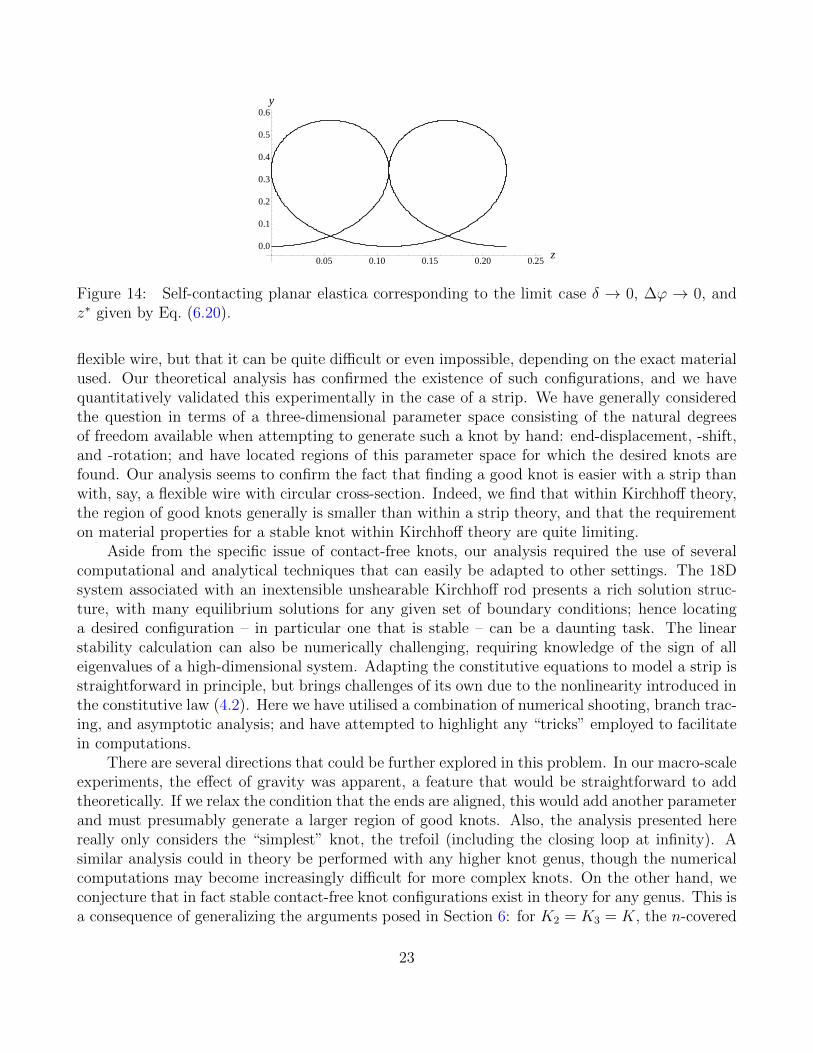
An alternative way of viewing the analytical expressions is to fix δ and plot the boundarycurves in the ∆ϕ-z∗ plane. These analytical curves are compared with numerical computationsin Figure 13-Left. The numerical computations follow configurations with one self-contact point,as for curve X1 in Figure 7-right. The crossing of curve I and II happens at z∗ = 0.382, a valueindependent of δ. This is an approximation of the maximum z∗ point on the numerical curve, seeFigure 13-Left. We see in Figure 13-Right that on numerical curves, this maximum point onlyvery slowly depends on δ, and that as δ → 0, this point converge towards z∗ ' 0.223. This limitvalue may be computed as the end-to-end distance of a self-contacting planar elastica, see [28]and Figure 14. It is the solution of

0 = E (3π/4,m)−(

1− m

2

)F (3π/4,m) (6.19)

z∗ = 1− 2

m

[1− E(π/2,m)

F(π/2,m)

](6.20)

where m ' −5.4, F(x,m) is the incomplete elliptic integral of the first kind, and E(x,m) is theincomplete elliptic integral of the second kind.

7 Discussion

In this paper we have explored the possibility of generating stable knot configurations of an elasticrod or strip in a clamped geometry and with no points of self-contact. One motivation for thisstudy was the simple observation that such configurations can be replicated with a strip of paper or

22

0.05 0.10 0.15 0.20 0.25z

0.0

0.1

0.2

0.3

0.4

0.5

0.6y

Figure 14: Self-contacting planar elastica corresponding to the limit case δ → 0, ∆ϕ → 0, andz∗ given by Eq. (6.20).

flexible wire, but that it can be quite difficult or even impossible, depending on the exact materialused. Our theoretical analysis has confirmed the existence of such configurations, and we havequantitatively validated this experimentally in the case of a strip. We have generally consideredthe question in terms of a three-dimensional parameter space consisting of the natural degreesof freedom available when attempting to generate such a knot by hand: end-displacement, -shift,and -rotation; and have located regions of this parameter space for which the desired knots arefound. Our analysis seems to confirm the fact that finding a good knot is easier with a strip thanwith, say, a flexible wire with circular cross-section. Indeed, we find that within Kirchhoff theory,the region of good knots generally is smaller than within a strip theory, and that the requirementon material properties for a stable knot within Kirchhoff theory are quite limiting.

Aside from the specific issue of contact-free knots, our analysis required the use of severalcomputational and analytical techniques that can easily be adapted to other settings. The 18Dsystem associated with an inextensible unshearable Kirchhoff rod presents a rich solution struc-ture, with many equilibrium solutions for any given set of boundary conditions; hence locatinga desired configuration – in particular one that is stable – can be a daunting task. The linearstability calculation can also be numerically challenging, requiring knowledge of the sign of alleigenvalues of a high-dimensional system. Adapting the constitutive equations to model a strip isstraightforward in principle, but brings challenges of its own due to the nonlinearity introduced inthe constitutive law (4.2). Here we have utilised a combination of numerical shooting, branch trac-ing, and asymptotic analysis; and have attempted to highlight any “tricks” employed to facilitatein computations.

There are several directions that could be further explored in this problem. In our macro-scaleexperiments, the effect of gravity was apparent, a feature that would be straightforward to addtheoretically. If we relax the condition that the ends are aligned, this would add another parameterand must presumably generate a larger region of good knots. Also, the analysis presented herereally only considers the “simplest” knot, the trefoil (including the closing loop at infinity). Asimilar analysis could in theory be performed with any higher knot genus, though the numericalcomputations may become increasingly difficult for more complex knots. On the other hand, weconjecture that in fact stable contact-free knot configurations exist in theory for any genus. This isa consequence of generalizing the arguments posed in Section 6: for K2 = K3 = K, the n-covered

23

ring is stable if K ≥ n, and knots of increasing genus are (likely) nearby the n-covered ring. Ofcourse, it remains to be seen via either formal asymptotic analysis about the n-covered ring forn > 2 and/or numerical computation whether such regions of parameter space can explicitly befound. Here we restricted our analysis to the values K2 = K3 = 3, a choice that ensured stability ofthe doubly-covered ring but that required a Poisson ratio of negative 1/2 in an elliptical geometry.While fixing these parameters created a more manageable parameter space to explore, from atheoretical point of view good knots of a given genus will be attainable in a rod framework overregions of the K2-K3 space. Whether such regions are physically realizable is a separate issue:while K2 can be computed for any geometry using simple formulae for second moment of area,and can in theory be made to take on any positive value, the torsional rigidity constant thatdetermines K3 is much more difficult to compute and has only been determined for a very smallnumber of cross-section geometries [38, 23].

A final direction of interest for future study is to connect to polymer mechanics. As noted inthe introduction, there is an abundance of knots found in polymers in biology, and in numerousinstances the presence of self-contact is an important feature underlying the biological activity.Our analysis suggests that it may be possible for a knotted polymer to have no points of self-contact, but that such situations would be rarely encountered; this raises the interesting questionsof whether such configurations do occur and if so what is the impact on the biological function.

8 Acknowledgements

The authors thank A. Goriely for discussions and support, P. Pieranski for mentioning the problemof stable knots, and E. Starostin for providing the Lurie reference. S.N. acknowledges supportfrom the U.K. Royal Society through the International Exchanges Scheme (grant IE120203), andfrom the french Agence Nationale de la Recherche through grants ANR-13-JS09-0009 and ANR-14-CE07-0023-01.

A Full system

We provide here the full set of equations in component form for the dynamical system, equilibriumconfigurations, and the linear stability system.

24

Dynamical system. The dynamical system consists of the force and moment balance (2.1),the moving frame equations, (2.2), as well as r′ = d3. In component form these read

x′ = d3x , n′1 = n2 u3 − n3u2 − f1 + ρA (x d1x + y d1y + z d1z) (A.1a)

y′ = d3y , n′2 = n3 u1 − n1u3 − f2 + ρA (x d2x + y d2y + z d2z) (A.1b)

z′ = d3z , n′3 = n1 u2 − n2u1 − f3 + ρA (x d3x + y d3y + z d3z) (A.1c)

d′3x = u2 d1x − u1 d2x , m′1 = m2 u3 −m3u2 + n2 (A.1d)

d′3y = u2 d1y − u1 d2y , m′2 = m3 u1 −m1u3 − n1 (A.1e)

d′3z = u2 d1z − u1 d2z , m′3 = m1 u2 −m2u1 (A.1f)

d′1x = u3 d2x − u2 d3x , d′2x = u1 d3x − u3 d1x (A.1g)

d′1y = u3 d2y − u2 d3y , d′2y = u1 d3y − u3 d1y (A.1h)

d′1z = u3 d2z − u2 d3z , d′2z = u1 d3z − u3 d1z. (A.1i)

Equilibrium system. Setting time derivatives to zero and denoting equilibrium variables withindex e, we have the system

x′e = d3xe , n′1e = n2e u3e − n3eu2e − f1 (A.2a)

y′e = d3ye , n′2e = n3e u1e − n1eu3e − f2 (A.2b)

z′e = d3ze , n′3e = n1e u2e − n2eu1e − f3 (A.2c)

d′3xe = u2e d1xe − u1e d2xe , m′1e = m2e u3e −m3eu2e + n2e (A.2d)

d′3ye = u2e d1ye − u1e d2ye , m′2e = m3e u1e −m1eu3e − n1e (A.2e)

d′3ze = u2e d1ze − u1e d2ze , m′3e = m1e u2e −m2eu1e (A.2f)

d′1xe = u3e d2xe − u2e d3xe , d′2xe = u1e d3xe − u3e d1xe (A.2g)

d′1ye = u3e d2ye − u2e d3ye , d′2ye = u1e d3ye − u3e d1ye (A.2h)

d′1ze = u3e d2ze − u2e d3ze , d′2ze = u1e d3ze − u3e d1ze (A.2i)

whereu1e = m1e, u2e =

m2e

K2

, u3e =m3e

K3

. (A.3)

Stability system. Following the perturbation scheme outlined in the main text, the eigenvaluesω that determine stability are determined from the following set of 12 equations

x′ = α2 d1xe − α1 d2xe , n′1 = n2e u3 + n2 u3e − n3eu2 − n3u2e − ω2 (x d1xe + y d1ye + z d1ze)

y′ = α2 d1ye − α1 d2ye , n′2 = n3e u1 + n3 u1e − n1eu3 − n1u3e − ω2 (x d2xe + y d2ye + z d2ze)

z′ = α2 d1ze − α1 d2ze , n′3 = n1e u2 + n1 u2e − n2eu1 − n2u1e − ω2 (x d3xe + y d3ye + z d3ze)

α′1 = u1 + u3e α2 − u2e α3 , m′1 = m2e u3 + m2 u3e −m3eu2 − m3u2e + n2

α′2 = u2 + u1e α3 − u3e α1 , m′2 = m3e u1 + m3 u1e −m1eu3 − m1u3e − n1 (A.4)

α′3 = u3 + u2e α1 − u1e α2 , m′3 = m1e u2 + m1 u2e −m2eu1 − m2u1e.

25

B Asymptotic approach

We here detail the asymptotic approach to compute the parameter value for which knotted con-figurations exist near the point z∗ = 0, ∆ϕ = 0, δ = 0, see Section 6. For Elastic Strips, thedoubly covered ring is stable [3], while for Kirchhoff rods, stability of the n-covered ring has beenestablished analytically [24] as a function of material parameters K2, K3, yielding the result thatthe configuration is stable if and only if√

K2 − 1

K2

K3 − 1

K3

≥ n− 1

n. (B.1)

In the case of the doubly-covered ring, with n = 2, and with K2 = K3, (B.1) simply readsK2 = K3 ≥ 2 for stability. If this is satisfied, then since knotted configurations exist nearby, it isreasonable to expect that these knotted configurations will be stable. We introduce the notationk2 = 1 − 1/K2 and k3 = 1 − 1/K3 and we present results valid for both the Elastic Strip andKirchhoff rod models, as well as for both curves I and II. (Formally, the Elastic Strip case isrecovered by setting k2 = 1 and k3 = 1/2.) We uses (X,Z,X) Euler angles (ψ, θ, φ) where thematerial frame is given by

{d1,d2,d3}T =M · {e1, e2, e3}T (B.2)

with

M =

− cosφ sin θ cos θ cosφ cosψ − sinφ sinψ cosψ sinφ+ cos θ cosφ sinψsin θ sinφ − cos θ cosψ sinφ− cosφ sinψ cosφ cosψ − cos θ sinφ sinψ

cos θ cosψ sin θ sin θ sinψ

(B.3)

The solution at order 0 is given by (6.6), (6.10), and (6.11). At order 1, one finds the force to be

n[1] = (n[1]x (0), 0, n

[1]τ (0))T while the moment and Darboux vectors are

m[1]x (s) = m[1]

x (0) +n[1]τ (0)

4π(1− cos(4πs)) u[1]x (s) = m[1]

x (s) (B.4)

m[1]t (s) =

(m[1]τ (0)− n

[1]x (0)

4π

)sin(4πs) u

[1]t (s) = 4π k2 φ

[1](s) + (1− k2)m[1]t (s) (B.5)

m[1]τ (s) =

n[1]x (0)

4π+

(m[1]τ (0)− n

[1]x (0)

4π

)cos(4πs) u[1]τ (s) = 4π k3 θ

[1](s) + (1− k3)m[1]τ (s) (B.6)

26

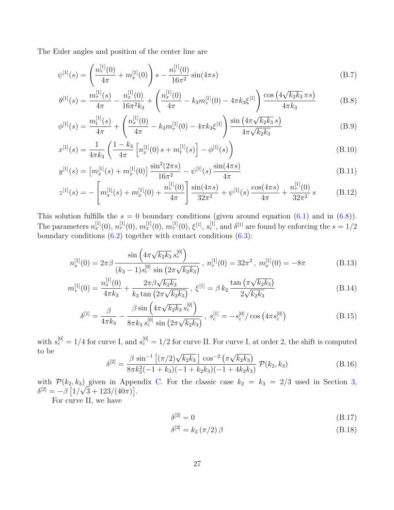
The Euler angles and position of the center line are

ψ[1](s) =

(n[1]τ (0)

4π+m[1]

x (0)

)s− n

[1]τ (0)

16π2sin(4πs) (B.7)

θ[1](s) =m

[1]τ (s)

4π− n

[1]x (0)

16π2k3+

(n[1]x (0)

4π− k3m[1]

τ (0)− 4πk3ξ[1]

)cos(4√k2k3 πs

)4πk3

(B.8)

φ[1](s) =m

[1]t (s)

4π+

(n[1]x (0)

4π− k3m[1]

τ (0)− 4πk3ξ[1]

)sin(4π√k2k3 s

)4π√k2k3

(B.9)

x[1](s) =1

4πk3

(1− k3

4π

[n[1]x (0) s+m

[1]t (s)

]− φ[1](s)

)(B.10)

y[1](s) =[m[1]x (s) +m[1]

x (0)] sin2(2πs)

16π2− ψ[1](s)

sin(4πs)

4π(B.11)

z[1](s) = −

[m[1]x (s) +m[1]

x (0) +n[1]τ (0)

4π

]sin(4πs)

32π2+ ψ[1](s)

cos(4πs)

4π+n[1]τ (0)

32π2s (B.12)

This solution fulfills the s = 0 boundary conditions (given around equation (6.1) and in (6.8)).

The parameters n[1]x (0), n

[1]τ (0), m

[1]x (0), m

[1]τ (0), ξ[1], s

[1]c , and δ[1] are found by enforcing the s = 1/2

boundary conditions (6.2) together with contact conditions (6.3):

n[1]x (0) = 2πβ

sin(

4π√k2k3 s

[0]c

)(k3 − 1)s

[0]c sin

(2π√k2k3

) , n[1]τ (0) = 32π2 , m[1]

x (0) = −8π (B.13)

m[1]τ (0) =

n[1]x (0)

4πk3+

2πβ√k2k3

k3 tan(2π√k2k3

) , ξ[1] = β k2tan(π√k2k3

)2√k2k3

(B.14)

δ[1] =β

4πk3−

β sin(

4π√k2k3 s

[0]c

)8πk3 s

[0]c sin

(2π√k2k3

) , s[1]c = −s[0]c / cos(4πs[0]c

)(B.15)

with s[0]c = 1/4 for curve I, and s

[0]c = 1/2 for curve II. For curve I, at order 2, the shift is computed

to be

δ[2] =β sin−1

[(π/2)

√k2k3

]cos−2

(π√k2k3

)8πk23(−1 + k3)(−1 + k2k3)(−1 + 4k2k3)

P(k2, k3) (B.16)

with P(k2, k3) given in Appendix C. For the classic case k2 = k3 = 2/3 used in Section 3,δ[2] = −β

[1/√

3 + 123/(40π)].

For curve II, we have

δ[2] = 0 (B.17)

δ[3] = k2 (π/2) β (B.18)

27

C The function P(k2, k3)

The function P(k2, k3) introduced in (B.16) is

P(k2, k3) = p1(k2, k3) cos

(1

2π√k2k3

)+ p2(k2, k3) cos

(5

2π√k2k3

)+

p3(k2, k3) sin

(1

2π√k2k3

)+ p4(k2, k3) sin

(3

2π√k2k3

)+

p5(k2, k3) sin

(5

2π√k2k3

)(C.1)

with

p1(k2, k3) = −π√k2 k3(−1 + k3)k3(1− 5k2k3 + 4k22k

23) (C.2)

p2(k2, k3) = p1(k2, k3) (C.3)

p3(k2, k3) = −10 + (19 + 46k2)k3 − (8 + 99k2 + 36k22)k23 + 16k2(3 + 5k2)k33 − 40k22k

43 (C.4)

p4(k2, k3) = 5− 11(1 + 2k2)k3 + (7 + 62k2 + 20k22)k23 − 15k2(3 + 4k2)k33 + 44k22k

43 (C.5)

p4(k2, k3) = (−1 + k3)(1− (1 + 4k2)k3 + 3k2k23 + 4k22k

33) (C.6)

D A generic configuration

We here give full details on the good-knot configuration shown in Figure 6-right. Initial valuesare n1(0) = −24.743, n2(0) = 17.772, n3(0) = 37.145, m1(0) = 7.5317, m2(0) = −8.7100,m3(0) = 4.529. Parameters are K = 3, z∗ = 0.115, δ = 0.05, ϕ/(2π) = 0.802, Tw = 0.107,W?

p = 3.695.

E A non-flip-symmetric configuration

We here give full details on a configuration which is not flip-symmetric. The initial values aren1(0) = −52.49, n2(0) = 4.12, n3(0) = 7.84, m1(0) = 2.21, m2(0) = −17.59, m3(0) = 10.01. Thesolution has K = 3, z∗ = 0.15, δ = 0.05, ϕ/(2π) = 0.785, Tw = 0.23,W?

p = 3.554, and is shown inFigure 15. The configuration is stable, knotted, and free of self-contact, but does not lie betweenwalls.

References

[1] Javier Arsuaga, Mariel Vazquez, Sonia Trigueros, De Witt Sumners, and Joaquim Roca.Knotting probability of dna molecules confined in restricted volumes: Dna knotting in phagecapsids. Proceedings of the National Academy of Sciences of the USA, 99(8):5373–5377, 2002.

[2] B. Audoly, N. Clauvelin, and S. Neukirch. Elastic knots. Physical Review Letters,99(16):164301, 2007.

28

Figure 15: A non-flip-symmetric configuration which is stable, knotted, and free of self-contact,but which does not lie between walls.

[3] Basile Audoly and Keith A. Seffen. Buckling of naturally curved elastic strips: The ribbonmodel makes a difference. Journal of Elasticity, 119(1):293–320, 2015.

[4] Mitchell A Berger and Chris Prior. The writhe of open and closed curves. Journal of PhysicsA: Mathematical and General, 39(26):8321–8348, 2006.

[5] Miklos Bergou, Max Wardetzky, Stephen Robinson, Basile Audoly, and Eitan Grinspun.Discrete elastic rods. ACM Transactions on Graphics (SIGGRAPH), 27(3):63:1–63:12, 2008.

[6] N. Clauvelin, B. Audoly, and S. Neukirch. Matched asymptotic expansions for twisted elasticknots: A self-contact problem with non-trivial contact topology. Journal of the Mechanicsand Physics of Solids, 57(9):1623–1656, 2009.

[7] B. D. Coleman and D. Swigon. Theory of supercoiled elastic rings with self-contact and itsapplication to DNA plasmids. Journal of Elasticity, 60:173–221, 2000.

[8] David J. Craik, Norelle L. Daly, Trudy Bond, and Clement Waine. Plant cyclotides: a uniquefamily of cyclic and knotted proteins that defines the cyclic cystine knot structural motif.Journal of molecular biology, 294(5):1327–1336, 1999.

[9] Marcelo A. Dias and Basile Audoly. A non-linear rod model for folded elastic strips. Journalof the Mechanics and Physics of Solids, 62:57–80, 2014.

[10] Marcelo A. Dias and Basile Audoly. ’Wunderlich, meet Kirchhoff’: A general and unifieddescription of elastic ribbons and thin rods. Journal of Elasticity, 119(1-2):49–66, 2015.

29

[11] D.J. Dichmann, Y. Li, and J.H. Maddocks. Hamiltonian formulations and symmetries inrod mechanics. In J.P. Mesirov, K. Schulten, and D.W. Sumners, editors, MathematicalApproaches to Biomolecular Structure and Dynamics, volume 82 of The IMA Volumes inMathematics and Its Applications, pages 71–113. Springer Verlag, 1996.

[12] G. Domokos and T. Healey. Hidden symmetry of global solutions in twisted elastic rings.Journal of Nonlinear Science, 11:47–67, 2001.

[13] Roger Fosdick and Eliot Fried, editors. The Mechanics of Ribbons and Moebius Bands.Springer, 2015.

[14] Alain Goriely, Michel Nizette, and Michael Tabor. On the dynamics of elastic strips. Journalof Nonlinear Science, 11(1):3–45, 2001.

[15] Alain Goriely and Michael Tabor. New amplitude equations for thin elastic rods. Phys. Rev.Lett., 77(17):3537–3540, 1996.

[16] Sachin Goyal, N. C. Perkins, and Christopher L. Lee. Non-linear dynamic intertwining ofrods with self-contact. International Journal of Non-Linear Mechanics, 43(1):65–73, 2008.

[17] T. J. Healey. Material Symmetry and Chirality in Nonlinearly Elastic Rods. Mathematicsand Mechanics of Solids, 7(4):405–420, 2002.

[18] Sophie E Jackson, Antonio Suma, and Cristian Micheletti. How to fold intricately: usingtheory and experiments to unravel the properties of knotted proteins. Current Opinion inStructural Biology, 42:6–14, 2017.

[19] Michal Jamroz, Wanda Niemyska, Eric J. Rawdon, Andrzej Stasiak, Kenneth C. Millett,Piotr Sukowski, and Joanna I. Sulkowska. Knotprot: a database of proteins with knots andslipknots. Nucleic Acids Research, 43(D1):D306–D314, 2015.

[20] M. K. Jawed, P. Dieleman, B. Audoly, and P. M. Reis. Untangling the mechanics and topologyin the frictional response of long overhand elastic knots. Phys. Rev. Lett., 115(11):118302,2015.

[21] Joel Langer and David A Singer. Knotted Elastic Curves in IR3. J. London Math. Soc.(2),30:512–520, 1984.

[22] Nicole C H Lim and Sophie E Jackson. Molecular knots in biology and chemistry. Journalof Physics: Condensed Matter, 27(35):354101, 2015.

[23] A. I. Lurie. Theory of elasticity. Foundations of Engineering Mechanics. Springer, 2005.

[24] Robert S. Manning and Kathleen A. Hoffman. Stability of n-covered circles for elastic rodswith constant planar intrinsic curvature. Journal of elasticity and the physical science ofsolids, 62(1):1–23, 2001.

30

[25] Davide Marenduzzo, Cristian Micheletti, Enzo Orlandini, and De Witt Sumners. Topologicalfriction strongly affects viral dna ejection. Proceedings of the National Academy of Sciencesof the USA, 110(50):20081–20086, 2013.

[26] Sebastien Neukirch, Joel Frelat, Alain Goriely, and Corrado Maurini. Vibrations of post-buckled rods: The singular inextensible limit. Journal of Sound and Vibration, 331(3):704 –720, 2012.

[27] Sebastien Neukirch and Michael E. Henderson. Classification of the spatial clamped elastica:symmetries and zoology of solutions. Journal of Elasticity, 68:95–121, 2002.

[28] M. Nizette and A. Goriely. Toward a classification of Euler-Kirchhoff filaments. Journal ofMathematical Physics, 40:2830–2866, 1999.

[29] P. Patricio, M. Adda-Bedia, and M. Ben Amar. An elastica problem: instabilities of an elasticarch. Physica D, 124:285–295, 1998.

[30] P. Pieranski, S. Przybyl, and A. Stasiak. Tight open knots. The European Physical JournalE, 6:123–128, 2001.

[31] Christopher B. Prior and Sebastien Neukirch. The extended polar writhe: a tool for opencurves mechancis. J. Phys. A: Math. Theo., 49:215201, 2016.

[32] V. Rossetto and A. C. Maggs. Writhing geometry of open DNA. Journal of Chemical Physics,118(21):9864–9874, 2003.

[33] F. Schuricht and H. von der Mosel. Euler-Lagrange equations for nonlinearly elastic rodswith self-contact. Archive for Rational Mechanics and Analysis, 168(1):35–82, 2003.

[34] E. L. Starostin. Equilibrium configurations of a thin elastic rod with self-contacts. PAMM,Proc. Appl. Math. Mech., 1(1):137–138, 2002.

[35] E. L. Starostin and G. H. M. van der Heijden. The shape of a mobius strip. Nature Materials,6(8):563–567, 2007.

[36] Joanna I. Sulkowska, Piotr Sulkowski, P. Szymczak, and Marek Cieplak. Stabilizing effect ofknots on proteins. Proceedings of the National Academy of Sciences, USA, 105(50):19714–19719, 2008.

[37] D. W. Sumners and S. G. Whittington. Knots in self-avoiding walks. J. Phys. A: Math. Gen.,21:1689–1694, 1988.

[38] S. Timoshenko and J.N. Goodier. Theory of elasticity. New York, 412:108, 1951.

[39] G. H. M van der Heijden, S. Neukirch, V. G. A. Goss, and J. M. T. Thompson. Instability andself-contact phenomena in the writhing of clamped rods. Int. J. Mech. Sci., 45(1):161–196,2003.

31

[40] Jeremiah R. Wagner, Joseph S. Brunzelle, Katrina T. Forest, and Richard D. Vierstra. A light-sensing knot revealed by the structure of the chromophore-binding domain of phytochrome.Nature, 438:325–331, 2005.

[41] Dungan J. M. Wasserman S. A. and Cozzarelli N. R. Discovery of a predicted DNA knotsubstantiates a model for site-specific recombination. Science, 22:171–174, 1985.

32