stabilized finite elements for compressible turbulent ... · pdf fileii.4 curved mesh...

STABILIZED FINITE ELEMENTS FOR COMPRESSIBLE

TURBULENT NAVIER-STOKES

By

Jon Taylor Erwin

W. Kyle AndersonProfessor of Computational Engineering(Chair)

Sagar KapadiaResearch Assistant Professor ofComputational Engineering(Committee Member)

Li WangResearch Assistant Professor ofComputational Engineering(Committee Member)

Kidambi SreenivasResearch Professor of ComputationalEngineering(Committee Member)

Clarence O. E. BurgAssociate Professor of Mathematics(Committee Member)

STABILIZED FINITE ELEMENTS FOR COMPRESSIBLE

TURBULENT NAVIER-STOKES

By

Jon Taylor Erwin

A Dissertation Submitted to the Faculty of the University ofTennessee at Chattanooga in Partial Fulfillment of

the Requirements of the Degree of Doctor ofPhilosophy in Computational Engineering

The University of Tennessee at ChattanoogaChattanooga, Tennessee

December 2013

ii

Copyright© 2013

By Jon Taylor Erwin

All Rights Reserved

iii

ABSTRACT

In this research a stabilized finite element approach is utilized in the development of a

high-order flow solver for compressible turbulent flows. The Reynolds averaged Navier-Stokes

(RANS) equations and modified Spalart-Almaras (SA) turbulence model are discretized using the

streamline/upwind Petrov-Galerkin (SUPG) scheme. A fully implicit methodology is used to ob-

tain steady state solutions or to drive unsteady problems at each time step. Order of accuracy is

assessed for inviscid and viscous flows in two and three dimensions via the method of manufac-

tured solutions. Proper treatment of curved surface geometries is of vital importance in high-order

methods, especially when high aspect ratio elements are used in viscous flow regions. In two

dimensions, analytic surface representations are used to ensure proper surface point placement,

and an algebraic mesh smoothing procedure is applied to prevent invalid elements in high aspect

ratio meshes. In dealing with complex three-dimensional geometries, high-order curved surfaces

are generated via a Computational Analysis PRogramming Interface (CAPRI), while the interior

meshes are deformed through a linear elasticity solver. In addition, the effects of curved elements

on solution accuracy are evaluated. Finally, several test cases in two and three dimensions are

presented and compared with benchmark results and/or experimental data.

iv

DEDICATION

This dissertation is dedicated to my loving and supportive wife, Tresa Erwin, and to our

wonderful daughter, Layla Erwin.

v

ACKNOWLEDGEMENTS

I would like to thank my adviser, Dr. W. Kyle Anderson, for his support and encouragement

in this endeavor. Sincere thanks also go to committee, Dr. Sagar Kapdia, Dr. Li Wang, Dr. Kidambi

Sreenivas, and Dr. Clarence O. E. Burg for serving on my dissertation committee and for providing

valuable insights throughout this research. I would also like to thank Dr. Timothy Swafford for

being a constant source of guidance and encouragement throughout my time at the SimCenter.

Additionally, I owe a debt of gratitude to the entire SimCenter faculty and staff for providing an

open and friendly environment for research.

I would also like to thank my parents, Rex and Evonna Lynn and Dennis and Andrea Erwin,

for all of their support an encouragement. Finally, I would like to thank my wife, Tresa, without

whose patience and support none of this would have been possible.

vi

TABLE OF CONTENTS

ABSTRACT.................................................................................................................................... iv

DEDICATION ................................................................................................................................. v

ACKNOWLEDGEMENTS ............................................................................................................ vi

LIST OF TABLES .......................................................................................................................... ix

LIST OF FIGURES ......................................................................................................................... x

CHAPTER

I. INTRODUCTION ............................................................................................................... 1

Motivation............................................................................................................................ 2Outline ................................................................................................................................. 8

II. METHODOLOGY ............................................................................................................ 10

Governing Equations ......................................................................................................... 10Discretization ..................................................................................................................... 14Mesh Curving Strategy ...................................................................................................... 21

Two Dimensions .......................................................................................................... 21Three Dimensions ........................................................................................................ 26

Wall Distance ..................................................................................................................... 30

III. CODE VERIFICATION .................................................................................................... 35

Two Dimensions ................................................................................................................ 37Three Dimensions .............................................................................................................. 41

IV. CURVED ELEMENTS ..................................................................................................... 44

vii

V. NUMERICAL RESULTS.................................................................................................. 58

Two Dimensions ................................................................................................................ 58Laminar Flow Over NACA 0012................................................................................. 58Inviscid Flow Over NACA 0012.................................................................................. 63Time-Accurate Cylinder .............................................................................................. 64

Three Dimensions .............................................................................................................. 69Delta Wing ................................................................................................................... 69Viscous flows over a three-dimensional circular cylinder ........................................... 73Turbulent Flow Over an ONERA M6 Swept Wing ..................................................... 76Turbulent Flow over a NASA Trap Wing .................................................................... 78

VI. CONCLUSION.................................................................................................................. 85

Summary............................................................................................................................ 85Recommendations for Future Work................................................................................... 87

REFERENCES .............................................................................................................................. 88

VITA .............................................................................................................................................. 95

viii

LIST OF TABLES

I.1 Relative work for PG and DG schemes for different element types and accuracyorder ......................................................................................................................... 7

III.1 Order of accuracy for the two-dimensional Euler equations ............................................. 39

III.2 Order of accuracy for the three-dimensional Euler equations ........................................... 43

IV.1 Order of accuracy on P1 uniform meshes.......................................................................... 48

IV.2 Order of accuracy on P2 uniform meshes.......................................................................... 48

IV.3 Order of accuracy on P1 curved meshes ............................................................................ 49

IV.4 Order of accuracy on P2 curved meshes ............................................................................ 50

IV.5 Order of accuracy for type 1 elements............................................................................... 52

IV.6 Order of accuracy for type 2 elements............................................................................... 53

IV.7 Order of accuracy study for parabolic mesh with viscous wall spacing............................ 56

V.1 Mesh statistics for NACA 0012 ......................................................................................... 62

ix

LIST OF FIGURES

I.1 Stencils for PG and DG schemes......................................................................................... 3

I.2 Ratio of Degrees of Freedom and Non-Zero Entries in Matrix for Full Linearization........ 6

II.1 Demonstration mesh for mesh curving strategy ................................................................ 24

II.2 Illustration of mesh curving strategy ................................................................................. 25

II.3 Mesh curving procedure .................................................................................................... 28

II.4 Curved mesh displacements for ONERA M6 swept wing geometry ................................ 29

II.5 Demonstration of mesh curving on ONERA M6 swept wing geometry ........................... 29

II.6 Demonstration of octree used for distance calculation...................................................... 33

II.7 Issue with nearest neighbor search .................................................................................... 34

III.1 Manufactured solution for compressible Euler and Navier-Stokes equations ................... 38

III.2 Coarse mesh used for manufactured solution .................................................................... 38

III.3 Observed order at varying Reynolds numbers ................................................................... 40

III.4 Manufactured solution for compressible Euler equations ................................................. 42

III.5 Observed order at varying Reynolds numbers ................................................................... 42

IV.1 Uniform hexahedral mesh.................................................................................................. 47

IV.2 Curved hexahedral mesh.................................................................................................... 49

IV.3 Elements for higher-order accuracy................................................................................... 51

x

IV.4 Grid Convergence on Meshes with Curved Elements ....................................................... 51

IV.5 Mesh and contours of y-displacement for parabolic mesh................................................ 54

IV.6 Creation of type 2 cells in the interior of the mesh............................................................ 57

V.1 Mach contours for NACA 0012, M∞ = 0.5, α = 3, Re = 5000....................................... 59

V.2 Results for laminar flow over NACA 0012 airfoil: M∞ = 0.5, α = 3, Re = 5000 .......... 60

V.3 Effect of stabilization matrices on skin friction coefficient ............................................... 63

V.4 Results for inviscid flow over NACA 0012 airfoil: M∞ = 0.5, α = 2 ............................. 64

V.5 Mesh for Circular Cylinder................................................................................................ 65

V.6 Contours of the x-component of velocity for impulsively started cylinder ....................... 66

V.7 Comparison of computed velocity profiles with experimental data .................................. 68

V.8 Mesh for low aspect ratio delta wing................................................................................. 69

V.9 Contours of total pressure .................................................................................................. 70

V.10 Cp plots at various stations along delta wing, linear elements........................................... 71

V.11 Cp plots at various stations along delta wing, quadratic elements..................................... 72

V.12 Computational mesh (containing 68,629 tetrahedral elements) for the three-dimensionalviscous flow over a circular cylinder ..................................................................... 73

V.13 Instantaneous velocities in the x-z plane (y=0) in the wake of the cylinder. 60contours are included from −0.2 to 0.2 ................................................................. 74

V.14 Normalized quantities in the wake of the circular cylinder using 3rd order SUPG(dashed line) in comparison with experimental data (circles) ............................... 75

V.15 ONERA M6 swept wing geometry.................................................................................... 76

V.16 Convergence history for P2 SUPG solution on ONERA M6 swept wing geometry......... 77

xi

V.17 Pressure coefficients plotted at various span-wise locations on the turbulent ONERAM6. Solid lines represent the CFL3D solution while dashed lines representthe SUPG solutions. The span-wise locations (as % semi-span) are indicatedabove each curve.................................................................................................... 77

V.18 Pressure coefficients at 65% semi-span for P2 solution on the linear mesh ...................... 78

V.19 Surface mesh for trap wing geometry................................................................................ 79

V.20 Turbulence working variable at three stations along trap wing configuration................... 80

V.21 Pressure coefficients at 17% semi-span on the NASA trap wing ...................................... 81







xii

CHAPTER I

INTRODUCTION

The development and application of Computational Fluid Dynamics (CFD) has evolved

to the point where very complicated flow fields can be computed for many steady and unsteady

scenarios. However, for many flows, success has been more limited by the severe computational

resources required to resolve small, but important flow features with sufficient accuracy. Poten-

tially significant advances for computing these flows can be achieved by using high-order spatial

discretization, coupled with adaptive meshing capabilities. For example, considering a typical

second-order scheme with truncation error of order h2, by assuming the same constant of propor-

tionality for the leading error term, a similar level of truncation error could be obtained using a

third-order scheme on a mesh with only N2/3 number of mesh points. To demonstrate the potential

impact, 71 million mesh points have recently been used for simulations over a nose landing gear

configuration using a second-order accurate scheme [1]. Using the (very) rough estimate provided

above, similar accuracy could be obtained using only 171 thousand nodes. Note, however, that on

a given mesh, the higher-order methods also have additional degrees of freedom and quadrature-

related function evaluations that must be accounted for to obtain a refined estimate of any potential

savings. While the above estimate is admittedly very optimistic and ignores the realities associated

with non-uniformly distributed truncation errors and having sufficient geometry resolution, success

1

in developing high-order schemes to a level of maturity where they can be used for production-level

simulations can have significant impact in many areas.

To this end, high-order discontinuous-Galerkin (DG) and Petrov-Galerkin (PG) algorithms

have been under development for several years. Globally, a significant level-of-effort has been

dedicated to the development of DG schemes [2–16], whereas much less effort has been dedicated

to the development of PG schemes [16–36].

While the DG method is conceptually simple to understand and many researchers have

obtained excellent results, the PG scheme offers some potential advantages when balancing the

level of work and computational resources required to obtain a solution.

Motivation

Before describing the PG methodology, motivation for studying the PG approach is pro-

vided by estimating the overall work involved in obtaining a solution for both the PG and the

DG schemes. To obtain the estimates, first consider a two-dimensional mesh that is assumed to

be regular and does not include any boundaries. The unknowns for the PG scheme are assumed

continuous across element boundaries, whereas for the DG scheme, unknowns are stored on a

per-element basis and are assumed to be discontinuous across element boundaries. Depictions for

a fourth-order accurate scheme are shown in figures I.1a and I.1b for the PG and DG schemes,

respectively. Using the configurations depicted in figure I.1, estimates for the number of degrees

of freedom and the number of non-zeros that would be required for a fully implicit algorithm can

be obtained for each scheme. Note that while the figure depicts configurations for fourth-order

accurate schemes, the estimates are derived below for arbitrary order.

2

(a) Stencil for fourth-order PGscheme

(b) Stencil for fourth-order DGscheme

Figure I.1 Stencils for PG and DG schemes

To obtain the estimates, note that for an algorithm of order p, an isolated triangle contains

ne = p − 1 mid-side degrees of freedom (DOF) along each edge (this does not include the vertices

at each end of the edge), ni = max(0, (p − 1)(p − 2)/2) degrees of freedom in the interior, and

nt = (p + 1)(p + 2)/2 total degrees of freedom. To determine the degrees of freedom for an

entire mesh, the PG scheme requires one DOF for each vertex plus ne × (number of edges), plus

ni × (number of triangles). Using an estimate that there are approximately twice as many edges

and triangles as there are nodes, the total DOF for a PG scheme is given as

DOFPG = NV + ne NE + ni NT ≈ NV (1 + 2ne + 2ni) (I.1)

where NV is the number of vertices in the mesh, NE is the number of edges in the mesh, and NT

is the number of triangles. Computing the DOF for the DG scheme is somewhat simpler because

the number of degrees of freedom for each triangle is given as 3 + 3ne + ni. Using the above

approximation that the number of triangles in the mesh is twice the number of vertices, the DOF

3

for a DG scheme is given as

DOFDG = NT (3 + 3ne + ni) ≈ 2NV (3 + 3ne + ni) (I.2)

Estimating the number of non-zero entries that are needed for a fully-implicit implementation is

achieved by noting that for a PG scheme, the number of connections for each vertex node in a

topologically regular mesh is given as

CPGv = 7 + 6ne + 6ne + 6ni (I.3)

where the term connection refers to a dependency relationship between nodes. Similarly, each

mid-edge node and interior node has the following number of connections

CPGe = 2nt − ne − 2 (I.4)

CPGi = nt (I.5)

The total number of non-zero entries in a matrix representing the full linearization of the residual is

determined by summing the connections for each entity multiplied by the total number of entities

in the mesh. Again, using the approximate relations between the number of edges and triangles in

a mesh, one obtains the following estimate

NNZPG = CPGv NV + CPG

e ne NE + CPGi ni NT

≈ NV(CPGv + 2CPG

e ne + 2CPGi ni

) (I.6)

4

For the DG scheme, estimating the number of non-zeros is again facilitated by first considering

each triangle individually and subsequently multiplying by the number of triangles. Here, the

number of connections for each vertex, mid-side node, and interior node, is given as

CDGv = nt + 2nt (I.7)

CDGe = nt + nt (I.8)

CDGi = nt (I.9)

Because a triangle has three vertices and three edges, the total storage for the number of non-zeros

in the mesh is given by

NNZDG = NT(3CDG

v + 3CDGe ne + CDG

i ni)

≈ 2NV(3CDG

v + 3CDGe ne + CDG

i ni) (I.10)

In three dimensions, a similarly canonical mesh is not available. However, by examining

several meshes for actual geometries, it is observed that there are approximately 13 edges that

connect to any vertex, with 21–23 tetrahedral elements connecting at a common node. Therefore,

to obtain the estimates for three dimensions, an icosahedron, which has 12 connecting edges and

20 connecting tetrahedrons, is used as a representative configuration.

Figure I.2 shows the ratio of the number of degrees of freedom for a DG scheme to that

of a PG scheme, as well as the ratio of the number of non-zero entries for both inviscid and

viscous flows. Note that when determining the ratio of non-zero entries in the matrix for inviscid

5

flows, the DG scheme only requires data immediately adjacent to the interface between triangles

or tetrahedra, whereas for viscous flows, all the data in each adjoining element is required. As

seen in the figure, for low orders of accuracy, the DG scheme requires significantly more degrees

of freedom and non-zero matrix entries than the PG scheme. Of particular interest is the fact that

for three-dimensional geometries, the DG scheme requires an order of magnitude more resources

than the PG scheme for linear and quadratic elements. Numerical experiments for electromagnetic

applications using both PG and DG formulations have verified these trends [37]. Note that in

reference [37], the DG scheme has been shown to exhibit as much as 40% lower errors on a given

mesh. However, the gains in accuracy are more than offset by the computing requirements.

0

1

2

3

4

5

6

7

8

0 2 4 6 8 10 12 14 16

1

Rat

io(D

G/P

G)

Polynomial Order

DOFNNZ (Euler)

NNZ (Navier-Stokes)

(a) Two dimensional estimates

0

5

10

15

20

25

30

0 2 4 6 8 10 12 14 16

1

Rat

io(D

G/P

G)

Polynomial Order

DOFNNZ (Euler)

NNZ (Navier-Stokes)

(b) Three dimensional estimates

Figure I.2 Ratio of Degrees of Freedom and Non-Zero Entries in Matrix for Full Linearization

Although the work estimates given above are quite relevant, they are not dispositive as to

which scheme will ultimately gain acceptance. First, more favorable work estimates for the DG

6

scheme can be obtained on non-tetrahedral meshes. As an example, Table I.1 shows results for lin-

ear and quadratic elements obtained by computing the degrees of freedom and non-zero entries on

a cubic volume subdivided into tetrahedral, hexahedral, and prismatic elements. In agreement with

the estimates above, the DG scheme requires significantly more unknowns and matrix elements

than the PG scheme for tetrahedrons. However, the DG scheme compares somewhat more favor-

ably for hexahedra, with prismatic elements falling in between. Other factors that will ultimately

determine the acceptance of these schemes include robustness, matrix conditioning, accuracy, and

computational effort required to compute the residuals and matrix entries.

Table I.1 Relative work for PG and DG schemes for different element types and accuracy order

Tetrahedron Hexahedron Prismatic

DOF Ratio NNZ Ratio DOF Ratio NNZ Ratio DOF Ratio NNZ Ratio

Linear 22.16 19.8 7.53 5.74 11.35 9.42Quadratic 7.19 6.20 2.92 2.14 4.02 3.15

As demonstrated in references [37] and [38] using the method of manufactured solutions,

the accuracy of the PG scheme appears to be somewhat better than the DG scheme when measured

against the number of degrees of freedom, while the DG scheme may have accuracy advantages

when compared to the PG scheme on the same mesh. The advantage of the PG scheme is most

significant for low-to-moderate orders of accuracy. In some applications, such as those that require

uniformly high-order accuracy throughout the flow field, it appears that the schemes are compara-

ble when balancing accuracy and work. However, for applications where significant portions of the

7

flow-field are discretized with low-to-moderate-order elements, the PG scheme should be consid-

ered as a means for obtaining numerical solutions; this would include adaptive meshing strategies

where low-order elements constitute the initial mesh.

Because of the significant potential advantages of the Petrov-Galerkin scheme, an existing

solver for inviscid flows, based on the work described in reference [37], will be extended to in-

clude viscous simulation capability for laminar and turbulent flows. In addition, the capability for

handling multiple element types will be added, as the inviscid solver currently uses on tetrahedral

elements.

Outline

In the remaining chapters, the extensions to the high-order streamline/upwind Petrov-

Galerkin (SUPG) solver for viscous flows and mixed element types is detailed. Chapter II presents

the methodology utilized in this research. This includes a brief presentation of the compress-

ible Navier-Stokes equations with a modified SA turbulence model as well as a description of the

SUPG discretization. In addition, strategies for generating curved high-order meshes in two and

three dimensions are presented. To end the chapter, a computationally efficient methodology for

calculating the distance to possibly curved surfaces is described. Chapter III presents the method

of manufactured solutions as a means of code verification. Results are shown demonstrating proper

order of accuracy characteristics for both two and three dimensional solutions. Next, Chapter IV

explores some issues that arise when using high-order schemes on curved meshes. Results from

several numerical test cases are presented in Chapter V. These results include time dependent and

8

steady state flows as well as inviscid, laminar, and turbulent results. Finally, conclusions are sum-

marized in Chapter VI and recommendations for future work are made.

9

CHAPTER II

METHODOLOGY

Governing Equations

The compressible Reynolds Averaged Navier-Stokes equations coupled with the one equa-

tion of the modified Spalart and Allmaras turbulence model [15, 39] can be written in the conser-

vative form as

∂Q(x , t)∂t

+ ∇ · (Fe(Q) − Fv (Q,∇Q)) = S(Q,∇Q) in Ω (II.1)

where Ω is a bounded domain. The vector of conservative flow variables Q, the inviscid and

viscous Cartesian flux vectors, Fe and Fv , are defined by

Q =

ρ

ρu

ρv

ρw

ρE

ρν

F xe =

ρu

ρu2 + p

ρuv

ρuw

(ρE + p)u

ρuν

Fye =

ρv

ρuv

ρv2 + p

ρvw

(ρE + p)v

ρv ν

F ze =

ρw

ρuw

ρvw

ρw2 + p

(ρE + p)w

ρwν

(II.2)

10

F xv =

0

τxx

τx y

τxz

uτxx + vτx y + wτxz + κ ∂T∂x

1σ µ(1 + ψ) ∂ ν∂x

Fyv =

0

τx y

τy y

τy z

uτx y + vτy y + wτy z + κ ∂T∂ y

1σ µ(1 + ψ) ∂ ν∂ y

F zv =

0

τxz

τy z

τzz

uτxz + vτy z + wτzz + κ ∂T∂z

1σ µ(1 + ψ) ∂ ν∂z

(II.3)

where ρ, p, and E denote the fluid density, pressure, and specific total energy per unit mass,

respectively. The vector u = (u, v , w) represents the Cartesian velocity vector and ν represents the

turbulence working variable in the modified SA model. The pressure is determined by the equation

of state for an ideal gas,

p = (γ − 1)(ρE − 1

2ρ(u2 + v2 + w2)

)(II.4)

where γ is defined as the ratio of specific heats, which is 1.4 for air. Temperature and thermal con-

ductivity are represented by T and κ, respectively, and are related to the total energy and velocity

11

as

κT = γ(µ

Pr+µT

Pr T

) (E − 1

2

(u2 + v2 + w2

))(II.5)

where Pr and PrT are the Prandtl and turbulent Prandtl number that are set to be 0.72 and 0.9

respectively. The fluid viscous stress tensor, τ, is defined for a Newtonian fluid as

τi j = (µ + µT )

∂ui

∂x j+∂u j

∂xi− 2

3∂uk

∂xkδi j

(II.6)

where δi j is the Kronecker delta and subscripts i, j, k refer to the Cartesian coordinate compo-

nents for x = (x , y , z). In addition, µ refers to the fluid dynamic viscosity and is obtained via

Sutherland’s law, while µT denotes a turbulence eddy viscosity, which is obtained by

µT =

ρν fv1 if ν ≥ 0

0 if ν < 0(II.7)

The source term, S, in equation (II.1) has zero components for the continuity, momentum and

energy equations, and takes the following form for the turbulence model equation [15, 39]

ST = cb1 Sµψ − cw1ρ fw

(µψ

ρd

)2

+1σ

cb2ρ∇ν · ∇ν − µ

ρσ(1 + ψ)∇ρ · ∇ν (II.8)

12

The parameters for the production and destruction components of the modified SA turbulence

model are given as

S =

S + S if S ≥ −cv2S

S +S(c2

v2 + cv3 S)

(cv3 − 2cv2)S − Sif S < −cv2S

S =√ω ·ω S =

µψ

ρκ2T d2

fv2 fv1 =ψ3

ψ3 + c3v1

fv2 = 1 − ψ

1 + ψ fv1

(II.9)

and

r =µψ

ρSκ2T d2

g = r + cw2(r6 − r) fw = g

1 + c6

w3

g6 + c6w3

1/6

(II.10)

respectively. Here ω denotes the vorticity vector, ∇ × u, while d refers to the distance to viscous

wall at a specific location and must account for the curvature of the actual boundaries. The variable

ψ in the equations is designed to remove the effects of a negative turbulence working variable on

the robustness of the turbulence model as it is discretized by a high-order spatial discretization

scheme. This variable ψ is given by

ψ =

0.05 ln(1 + e20X) if X ≤ 10

X if X > 10(II.11)

where

X =ρv

µ(II.12)

such that it remains positive or becomes zero as the turbulence working variable goes negative, thus

preventing the instability issue caused by unbounded turbulence eddy viscosity. The constants in

13

the modified SA model to close the main flow equations are given as

cb1 = 0.1355 σ = 2/3 cb2 = 0.622 κT = 0.41 cw1 =cb1

κ2T

+1 + cb2

σ

cw2 = 0.3 cw3 = 2 cv1 = 7.1 cv2 = 0.7 cv3 = 0.9

(II.13)

In the case of laminar flow, the governing equations reduce to the compressible Navier-Stokes

equations, where the turbulence model equation vanishes and the turbulence eddy viscosity in the

fluid viscous stress tensor and the thermal conduction terms is set to zero.

Discretization

The computational domainΩ is partitioned into a tessellation of non-overlapping elements,

such thatΩ =⋃

i Ωi, whereΩi refers to the volume of an element i in the computational mesh. The

Galerkin finite-element approximation is expanded as a series of Lagrangian basis functions [40],

φ j , and solution coefficients for element i as

Qi (x) =∑

j

Qi jφ j (x) (II.14)

Here, the summation is over the nodes comprising element i, where Qi is the value of the dependent

variables at the nodes of the element. Because the set of basis functions is defined in a master

element spanning between 0 < ξ, η, ζ < 1, a coordinate mapping from the reference to a physical

element is required. The reference-to-physical transformation and the corresponding Jacobian Ji

14

associated with each element i are given by

xi =∑

j

xi jφ j (ξ, η, ζ ) Ji =

∂ x∂ξ

∂ x∂η

∂ x∂ζ

∂ y∂ξ

∂ y∂η

∂ y∂ζ

∂ z∂ξ

∂ z∂η

∂ z∂ζ

(II.15)

where xi represent the element-wise geometric mapping coefficients.

In the streamline/upwind Petrov-Galerkin method [16–36] the system of equations is writ-

ten as a weighted residual scheme,

0 =

$Ω

φ

[∂Q

∂t+ ∇ ·

(Fe (Q) − Fv (Q,∇Q)

)− S(Q,∇Q)

]dΩ

+∑

i

$Ωi

[(∂φ

∂x[A] +

∂φ

∂ y[B] +

∂φ

∂z[C]

)[τ]

(∂Q

∂t+ ∇ ·

(Fe (Q) − Fv (Q,∇Q)

)− S(Q,∇Q)

)]dΩi

(II.16)

where [A], [B], and [C] are the inviscid flux Jacobians, and [τ] is the stabilization matrix [17].

The weighting function, φ, is defined using the same basis functions as the dependent variables

so that without the stabilizing term a Galerkin-type method would result. The stabilization term

is added to compensate for a lack of dissipation in the stream-wise direction, thereby preventing

oscillations that commonly plague the Galerkin method for convection-dominated flows. Note

that in the stabilization term, the integration is strictly over the element interiors due to lack of

differentiability of the basis functions at the element boundaries. For inviscid flows, [τ] can be

15

obtained using the following definitions [41]:

[τ]−1 =∑

i

∣∣∣∣∣∂φi

∂x[A] +

∂φi

∂ y[B] +

∂φi

∂z[C]

∣∣∣∣∣ (II.17)

∣∣∣∣∣∂φi

∂x[A] +

∂φi

∂ y[B] +

∂φi

∂z[C]

∣∣∣∣∣ = [T ][Λ][T ]−1 (II.18)

where [T ] is the matrix of right eigenvectors and [Λ] is the diagonal matrix of eigenvalues of

the left hand side of equation (II.18). Note that many alternative stabilization matrices can be

derived using flux functions often used in finite-volume schemes [35]. Specifically, flux functions

such as flux-vector splitting [42–44] can be written as a sum of contributions, f + and f −, whose

eigensystems have positive and negative eigenvalues, respectively. Using these definitions, the

absolute value matrix in equations (II.17) and (II.18) can be replaced by the difference of ∂ f +

∂Q and

∂ f −∂Q . Potential advantages of this approach are that differentiability, positivity, and conservation of

total enthalpy [35, 45, 46] can be maintained.

For viscous flows, additional terms are required as the Reynolds number is decreased and

the viscous terms become dominant [16, 47, 48]. The reason for this modification is that the

weighted residual formulation, given in equation (II.16), requires that second derivatives be eval-

uated for the viscous flux term that is multiplied by the stabilization matrix. The evaluation of

this term results in a discretization that is one order less than the nominal order of the rest of the

scheme. As a consequence, when the viscous terms become dominant, the stabilization matrix

must behave as O(h2) instead of O(h) for the matrix described above. Theoretical analysis for

scalar equations results in applying a multiplicative scaling to the stabilization parameter based on

16

the local Peclet number (an excellent discussion can be found in reference [49]). In the current

research however, attempts to extend this methodology to systems of equations in a manner that

maintains the proper order of accuracy has not proven to be robust.

The form of stabilization matrix used here is very similar to that given in reference [47],

and can be motivated by first considering a scalar convection-diffusion equation given as

a∂u∂x− ∂

∂x

(ν∂u∂x

)= a

∂u∂x− ∂

∂x( fv ) = 0 (II.19)

where a is the convection speed and ν is the diffusion coefficient. An inviscid stabilization term

that corresponds to that described in equation (II.17) is given by

τ−1 =∑

i

∣∣∣∣∣∂φi

∂xa∣∣∣∣∣ (II.20)

Here, it is evident that τ varies as O(h), which is appropriate for the inviscid case but does not

have the proper limiting behavior for viscous dominated cases. To achieve the proper asymptotic

behavior, a viscous modification can be added so that τ−1 is now given as

τ−1 =∑

i

(∣∣∣∣∣∂φi

∂xa∣∣∣∣∣ +

∂φi

∂xν∂φi

∂x

)(II.21)

Here, it is apparent that the two terms comprising τ−1 vary as |a/L | and ν/L2, respectively, so that

a proportionality relationship for τ can be written as

τ ∝ L2

|aL | + ν(II.22)

17

With this formulation, when the convection term dominates, τ exhibits the O(h) property, whereas

for viscous dominated cases, τ varies as O(h2), which is the desired behavior.

To extend this approach to systems of equations, first note that the viscous flux in equa-

tion (II.19) can be written as

fv = ν∂u∂x

(II.23)

so that ν in equation (II.21) can be expressed as

ν =∂ fv∂

(∂u∂x

) (II.24)

Extending this methodology to systems is accomplished by noting that the viscous terms for the

Navier-Stokes equations can be written in the form

F xv = G1 j

∂Q

∂x j, F

yv = G2 j

∂Q

∂x j, F z

v = G3 j∂Q

∂x j(II.25)

where, for example

G11 =∂F x

v

∂(∂Q∂x

) , G12 =∂F x

v

∂(∂Q∂ y

) , G13 =∂F x

v

∂(∂Q∂z

) (II.26)

18

The resulting form for the viscous contribution to the stabilization matrix is finally given as

[τv]−1 =∑

i

[∂φi

∂x∂φi

∂ y

∂φi

∂z

]

G11 G12 G13

G21 G22 G23

G31 G32 G33

∂φi

∂x∂φi

∂ y

∂φi

∂z

(II.27)

This formulation has the advantage that a mesh spacing parameter is not required and the transition

from an inviscid- to a viscous-dominated stabilization matrix occurs naturally and is consistent

with the discretization of the governing equations.

For inviscid flows, boundary conditions are applied weakly by converting the volume inte-

gral involving the flux terms in the first integral in equation (II.16) into a surface integral using the

divergence theorem as

0 =∑

i

$Ωi

[φ∂Q

∂t+ ∇φ ·

(Fe (Q) − Fv (Q,∇Q)

)− φS(Q,∇Q)

]dΩi

+

"∂Ωi∩∂Ω

φ(Fe (Q) − Fv (Q,∇Q)

)· n dΓ

+∑

i

$Ωi

[(∂φ

∂x[A] +

∂φ

∂ y[B] +

∂φ

∂z[C]

)[τ]

(∂Q

∂t+ ∇ ·

(Fe (Q) − Fv (Q,∇Q)

)− S(Q,∇Q)

)]dΩi

(II.28)

and subsequently evaluating the flux at the wall using zero normal velocity. A similar procedure

is used for viscous flows with the exception that the velocities and turbulence working variable are

currently set to zero on no-slip walls and a constant temperature assumption is used.

19

After discretization, the system of nonlinear algebraic equations is solved using a Newton-

type method where the linear system is solved at each step using the Generalized Minimal Resid-

ual (GMRES) method [50] with ILU(k) preconditioning [51]. In addition, the three-dimensional

parallel flow solver uses the standard MPI message-passing library for inter-processor communi-

cation [52] and meshes are partitioned using the METIS mesh partitioner [53].

For time-dependent flows, time integration is performed via an implicit, second-order back-

ward difference formula (BDF2). For steady state problems, a local time-stepping method based

on CFL number is incorporated to alleviate the stiffness of the system in the initial stages of the

calculation. In many turbulent flow cases [54, 55], a simple CFL strategy has proven adequate,

though not ideal, for achieving steady state convergence. In order to maintain stability in the tran-

sient solution, a constant CFL of one was maintained while the L2 norm of the turbulence working

variable residual continued to rise. When the turbulence residual began to decrease, the CFL was

increased linearly to some maximum value, typically in the range of 100–200. Here, an attempt has

been made to automate this procedure following a similar approach as described in reference [56].

In particular, the CFL at each time step is increased or decreased by a factor related to the change

in the L2 residual norm. At time step n the CFL is given by

CFLn = min

CFLn−1 ·β‖Rn−1 ‖2−‖Rn ‖2‖Rn−1 ‖2 ,CFLmax

(II.29)

for some value β > 1. In the present work a value of β = 2 was used exclusively.

20

Mesh Curving Strategy

In the present work, each case begins with a P1 (linear) mesh, where all element boundaries

are linear. Additional nodes are then added to each element to generate a higher-order mesh. For

strictly flat surfaces, this poses no problem. For curved surfaces, however, care must be taken

to snap any new surface nodes to the original geometry. For anisotropic boundary-layer elements,

surface snapping poses a problem in and of itself. With high aspect ratio elements, surface snapping

alone often creates negative volumes; a means of displacing the interior nodes of the mesh is

needed.

Two Dimensions

In two dimensions, curved boundaries are recaptured using the analytic definition of each

boundary. For each case involving curved boundaries, additional code is required to snap higher

order nodes to the original surface.

Next, a means of displacing interior nodes is required. The methodology outlined by Allen

[57] is chosen because it is computationally efficient and easily implemented. For each mesh point,

denoted p, the distance to each of the nsurf curved surfaces, as well as to the far-field surface, are

computed. The distance to each curved surface is defined as

Sp,ns =∣∣∣xp − xp,ns

∣∣∣ (II.30)

21

where 1 ≤ ns ≤ nsurf , xp is the position of point p, and xp,ns is the position of the point on surface

ns closest to point p. Similarly, the far-field distance for each point is defined as

SpF =

∣∣∣∣xp − xpfarfield

∣∣∣∣ (II.31)

From these quantities, a normalized distance scale is defined between each mesh point and curved

surface as

ψp,ns =Sp,ns

SpF + Sp,ns

(II.32)

To deal with multiple curved surfaces, the displacement of each mesh point is defined based

on a weighted combination of the displacements of the nearest point on each surface. As such, it

is necessary to define the quantities

Spmin = min

1≤ns≤nsurfSp,ns

Sp,nssurf =

Spmin

Sp,ns

(II.33)

Smooth surface weighting functions are then defined as

SpTotal =

nsurf∑

ns=1

(Sp,ns

surf

) ssc

ϕp,ns =Sp,ns

surf

SpTotal

(II.34)

22

Finally, the displacement of each mesh point is computed as

∆xp =

nsurf∑

ns

ϕp,ns (1 − ψp,ns)st∆xp,ns (II.35)

where st controls the decay of the displacements away from the curved surface(s). Typical values

for st range from 2 to 5, with negligible differences in the resulting displacements. The multi-

surface scaling exponent ssc is not utilized since multiple curving surfaces are not needed in the

present work. For elements with interior nodes, the locations of these nodes are not determined

using the above procedure. Instead, coefficients for hierarchical basis functions are first determined

using the nodes on the boundary of the element, and the coordinates of the interior nodes are

determined by evaluating the basis functions at the appropriate positions in the reference element.

This procedure minimizes non-linearity in the mapping between the reference and physical spaces

that otherwise occurs if the interior nodes are positioned independently.

To illustrate the current mesh curving strategy, a demonstration mesh, shown in figure II.1,

is considered for a circular geometry with viscous spacing normal to the surface of 1 × 10−3.

Figure II.2 shows a close-up view of the viscous boundary layer at various stages.

23

Figure II.1 Demonstration mesh for mesh curving strategy

24

(a) initial mesh (b) snapped mesh (c) final mesh

Figure II.2 Illustration of mesh curving strategy

25

Three Dimensions

While the strategy outlined above for capturing curved geometry is adequate for two di-

mensional cases, a more robust procedure is required for dealing with complex, three dimensional

geometries. Developing new code on a case-by-case basis becomes impractical at best. To that

end, three dimensional curved meshes are generated through a parametric definition provided by

an external CAD engine. In particular, higher order points are projected onto the true geometry

using CAPRI (Computational Analysis PRogramming Interface) [58]. CAPRI provides a pro-

gramming interface for interrogating various commercial CAD engines. By providing access to

the native parametric surface definition, CAPRI facilitates the projection of higher-order points

onto a curved surface.

The mesh generating procedure begins with a CAD defined geometry. Similarly to the two

dimensional case, a traditional linear mesh is generated on the geometry. Additional points are

inserted into the linear mesh naively and then projected onto the CAD surface using CAPRI. To

accommodate the properly curved surface elements, interior elements in the boundary layer are

required to deform to avoid the generation of negative Jacobians. Here we make use of modified

linear elasticity theory [59] which assumes that the computational mesh obeys the isotropic linear

26

elasticity relations, taken in the following form:

∂

∂x

[d11

∂δx

∂x+ d12

∂δy

∂ y+ d13

∂δz

∂z

]+

∂

∂ y

[d44

(∂δx

∂ y+∂δy

∂x

)]+∂

∂z

[d66

(∂δx

∂z+∂δz

∂ y

)]= 0

∂

∂x

[d44

(∂δx

∂ y+∂δy

∂x

)]+

∂

∂ y

[d21

∂δx

∂x+ d22

∂δy

∂ y+ d23

∂δz

∂z

]+∂

∂z

[d55

(∂δy

∂z+∂δz

∂x

)]= 0

∂

∂x

[d66

(∂δx

∂z+∂δz

∂x

)]+

∂

∂ y

[d55

(∂δy

∂z+∂δz

∂ y

)]+∂

∂z

[d31

∂δx

∂x+ d32

∂δy

∂ y+ d33

∂δz

∂z

]= 0

(II.36)

where δ = (δx , δy , δz) denotes the nodal displacement vector in the Cartesian coordinate directions

and the coefficients, d, are defined as

d11 = d22 = d33 =E(1 − υ)

(1 + υ)(1 − 2υ)

d12 = d13 = d21 = d23 = d31 = d32 =Eυ

(1 + υ)(1 − 2υ)

d44 = d55 = d66 =E

2(1 + υ)

(II.37)

where E represents Young’s modulus and υ denotes Poisson’s ratio. Physically, Young’s modulus

is a measure of the stiffness of a material, while Poisson’s ratio is the ratio of transverse to axial

strain. As such, the values E and υ may be used to influence the deformation of the interior mesh.

In the present work, Poisson’s ratio is set to a constant value of υ = 0.3, while Young’s modulus is

set at each quadrature point to the inverse distance to the deforming surface. This strategy makes

sense given the nature of the particular problem being solved: the stiffest regions of the interior

mesh should be in the boundary layer near the solid wall. The overall mesh curving procedure is

outlined in the flowchart in figure II.3.

27

CADA water-tight

CAD definitionis required.

Linear MeshA linear mesh isgenerated using

the CADdefinition.

CAPRIHigher-order

points areinserted into thelinear mesh andprojected onto

the CADdefinition via a

CAPRIinterface.

Linear ElasticThe surface

displacementsprovided byCAPRI are

propogated intothe interior

domain via alinear elastic

solver.

Figure II.3 Mesh curving procedure

To demonstrate both the effectiveness and the shortcomings of this procedure, consider an

ONERA M6 swept wing mesh. Figure II.4 shows the projected geometry as well as the magnitude

of the displacement vector in a mid-span slice of the interior mesh. It is clear that the displacement

magnitude decays quickly as the distance from the wing increases. Additionally, the steps of the

mesh curving strategy are clearly demonstrated by looking closely at the leading edge of the wing

in figure II.5 as well as a cut of the interior mesh. In particular, figure II.5a shows the initial linear

mesh, while figure II.5b shows the projected surface mesh as it clearly crosses into the boundary

layer of the linear interior mesh. Finally, figure II.5c shows the valid final mesh.

Using the procedure described above, the majority of the interior mesh was deformed suc-

cessfully, although a small number of invalid elements could not be eliminated near the tip of the

swept wing. To circumvent this difficulty, the wing tip of the surface geometry was omitted from

the surface projection in order to obtain a valid mesh.

28

Figure II.4 Curved mesh displacements for ONERA M6 swept wing geometry

(a) Linear geometry. (b) Mesh overlapping when only thesurface is curved.

(c) Final mesh with curved interiorelements.

Figure II.5 Demonstration of mesh curving on ONERA M6 swept wing geometry

29

Wall Distance

In the source term of the modified SA turbulence model, given in equations (II.8) to (II.10),

the distance to the viscous wall is required at every point in the mesh. When dealing with higher

order curved geometry, it is important that these quantities reflect the curved surface definition.

As such, an efficient method for computing the distance to a curved three dimensional surface is

needed.

Given a point in space, xp, the nearest point on a parametric surface, S(ξ, η), occurs when

the vector between xp and S(ξ, η) is orthogonal to the surface. This is represented by a system of

two equations,

(S(ξ, η) − xp) · Sξ = 0

(S(ξ, η) − xp) · Sη = 0

(II.38)

where Sξ =∂S(ξ,η)∂ξ and Sη =

∂S(ξ,η)∂η . Therefore, finding the distance between a point and a surface

involves finding the roots, (ξ∗, η∗), of equation (II.38) via Newton’s method. The distance between

the point and the surface is then given as

d =∣∣∣S(ξ∗, η∗) − xp

∣∣∣ (II.39)

Since the surface elements are finite parametric surfaces, the root is only valid if it lies within the

parametric range of the element. When the root lies outside the range of the element, the nearest

point on the surface lies along an edge of the element. The procedure above is easily modified to

30

find the nearest point on a one-dimensional parametric edge. If the root on the edge lies outside

the parametric range of the edge, the nearest point on the edge lies at one of the endpoints.

Since this work is dealing with discrete computational meshes, the distance from any point

to a viscous wall involves finding the minimum distance amongst a large number of parametric

surfaces. Solving a root-finding problem for every mesh point/surface element pair quickly be-

comes impractical. In this work, an octree data structure is used to alleviate this problem. Given n

spatially defined objects, an octree is a data structure in which a three dimensional space is recur-

sively subdivided into ever smaller containers such that O(log n) tree traversal algorithms may be

utilized.

The octree begins as a cube encompassing all n objects. The cube is then subdivided into

eight equal octants that act as containers; each octant may contain any of the objects that lie com-

pletely within its bounds. This process continues recursively until some stopping criteria is met.

The octree drastically reduces the number of distance calculations that must be performed. For

each mesh point, the cost of finding the distance to the surface is reduced from O(n) to O(log n).

Even using the octree, many distance calculations must be performed between mesh points

and the viscous surface. Due to the expense of these calculations for curved surface elements,

surface points rather than surface elements are stored in the octree in this research. As such, for

each node in the mesh, a nearest neighbor search is carried out to find the nearest surface node.

From there, the elements and edges surrounding the nearest surface node are checked to find the

true minimum distance to the viscous surface.

Since points are dimensionless, an appropriate stopping criteria is needed to prevent indef-

inite recursion of the octree. In this work, a minimum number of objects must lie in a container

31

before that container is considered for subdivision. This strategy prevents the octree from becom-

ing too sparse as well. Through some brief experimentation, a minimum object count of 20 for

each container has proven adequate.

Once all points are inserted into the octree, each of the containers is contracted such that it

forms a minimum bounding box of the points within it or any of its sub-containers. This simple

process serves to minimize the number of containers that must be visited during nearest neighbor

searches. To illustrate this procedure, a non-trivial geometry is presented in figure II.6. This geom-

etry consists of 238,687 surface nodes and 476,429 surface triangles. The initial octree containing

all of the surface nodes is shown in figure II.6b and consists of 23,880 containers in 13 levels.

Finally, figure II.6c shows the final octree with contracted containers.

A potential problem arises from the choice to put the surface points, rather than the ele-

ments, into the octree. As illustrated in figure II.7 in two dimensions, the wrong node may be

found during the nearest neighbor search. Here, the nearest point on the surface is clearly on the

edge nearest node 101. The nearest surface node, however is node 41. During the subsequent

search through the neighboring edges of node 41, the proper face will never be checked. To avoid

this problem, a surface node is only considered during the nearest neighbor search if at least one

face connected to that node is visible from the point in question. Visibility is checked by exam-

ining the dot product between the outward-pointing unit normal vector of the face (at the surface

node) and the unit vector from the surface node to the mesh point. A positive dot product indicates

visibility.

Ultimately, the entire process described above must be performed in a parallel computing

environment. Initially, each process contains a portion of the computational mesh which may or

32

(a) Geometry definition

(b) Initial octree

(c) Contracted octree

Figure II.6 Demonstration of octree used for distance calculation

33

7

34129

101

Figure II.7 Issue with nearest neighbor search

may not include any viscous surfaces. To facilitate parallel distance computation, a surface mesh is

constructed on each process that contains only the surfaces of interest native to that process. These

surface meshes are then distributed to all processes such that each process has access to the full

surface mesh of interest. Each process then builds the complete octree for its copy of the surface

mesh. Finally, each process uses the octree to calculate the distance to the surface for each node it

owns. At this point, the octree is discarded since it is no longer needed.

34

CHAPTER III

CODE VERIFICATION

In the current work, the method of manufactured solutions is used extensively for code

verification. The method of manufactured solutions is a general procedure for generating non-

trivial exact solutions to a PDE or system of PDEs. Consider a PDE system in general form,

Du = S (III.1)

where D is the differential operator, u is the solution, and S is the source term. In order to find

an exact solution to this system, one chooses a source term and, using methods from applied

mathematics, inverts the differential operator to solve for u. With the method of manufactured

solutions, on the other hand, one chooses, or “manufactures,” a solution that is substituted into

the governing equations to obtain a source term S. This is accomplished by simply applying the

differential operator to the chosen solution.

Salari and Knupp [60] have outlined a comprehensive set of guidelines for choosing man-

ufactured solutions:

1. The manufactured solutions should be composed of smooth analytic functions. Possible

choices include polynomial, trigonometric, and exponential functions. This criteria ensures

35

that the solution can be easily computed at all spatial and temporal locations within the

computational domain.

2. The solution should be general enough to exercise every term in the governing equations.

3. The solution should have a sufficient number of non-trivial derivatives. For instance, when

verifying a code that is theoretically second order accurate, a linear solution would not pro-

vide a sufficient test since second order accuracy would be assured.

4. The solution should contain no singularities, discontinuities, or steep gradients. These would

require unnecessarily high grid resolution in order to obtain a converged solution.

It is important to note that the manufactured solution need not be physically realistic since the code

verification process is purely a mathematical exercise. In fact, non-physical solutions are much

easier to generate, and are therefore recommended for the method of manufactured solutions [60].

The observed order between a coarse and fine mesh is calculated via

p =log

(EcoarseEfine

)

log(

hcoarsehfine

) (III.2)

where E represents the L1, L2, or L∞ norm of the solution error. For a mesh with N degrees

of freedom, the mesh spacing is approximated as h (

1N

)1/2for two-dimensional flows and as

h (

1N

)1/3for three-dimensional flows.

36

Two Dimensions

To assess the order of accuracy for the two-dimensional Petrov-Galerkin code, trigonomet-

ric functions, given in equation (III.3) and shown in figure III.1, are used to derive the forcing

function.

ρ(x , y) = Aρ(1 + sin(πx) cos(πx) sin(πy) cos(πy)

)

u(x , y) = Au(1 + sin(2πx) cos(2πx) sin(2πy) cos(2πy)

)

v (x , y) = Av(1 + cos(2πx) cos(2πx) cos(2πy) cos(2πy)

)

T (x , y) = AT(1 + sin(2πx) sin(2πx) sin(2πy) sin(2πy)

)

(III.3)

In evaluating the order of accuracy, a series of sequentially refined meshes consisting of

585, 2193, and 8481 nodes are used where the coarsest mesh is shown in figure III.2. As seen, the

mesh consists of highly stretched triangles along the mid-section to represent spacings commonly

used for viscous flows. The normal spacings at the center of the coarse, medium, and fine meshes

are 1.2× 10−4, 6.0× 10−5, and 3.0× 10−5, respectively. It should be noted that similar experiments

have been conducted using meshes with near-equilateral triangles with similar results.

Table III.1 demonstrates the order of accuracy obtained for the Euler equations. As seen,

when linear (P1) and cubic (P3) polynomials are utilized, the design-order of accuracy is slightly

exceeded, whereas for quadratic (P2) polynomials it is slightly lower.

Recall that for the Petrov-Galerkin scheme, the stabilization matrix must be scaled properly

as the Reynolds number is decreased and the viscous terms become dominant. Figure III.3 depicts

the observed order of accuracy for schemes using linear, quadratic, and cubic polynomials over

37

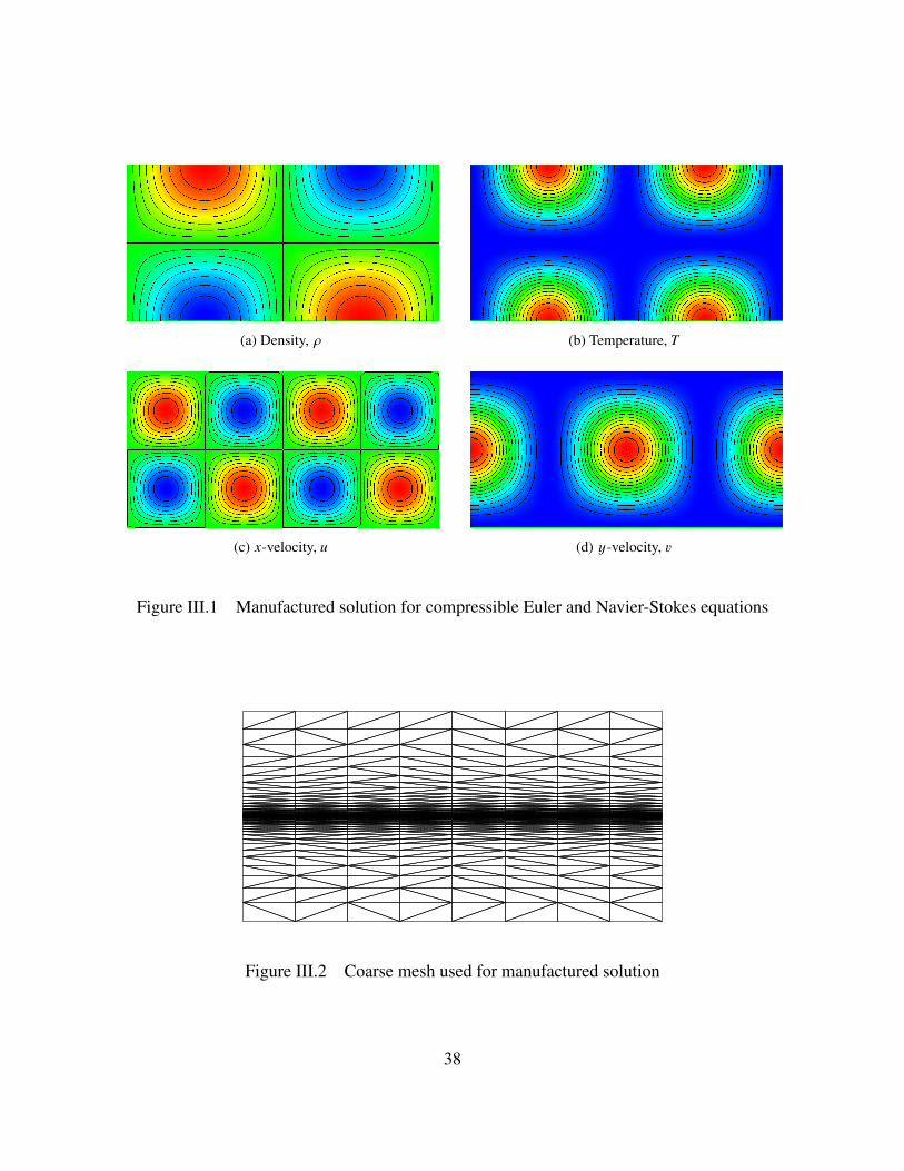
(a) Density, ρ (b) Temperature, T

(c) x-velocity, u (d) y-velocity, v

Figure III.1 Manufactured solution for compressible Euler and Navier-Stokes equations

Figure III.2 Coarse mesh used for manufactured solution

38

Table III.1 Order of accuracy for the two-dimensional Euler equations

Nodes in Mesh P1 Elements P2 Elements P3 Elements

L1 L2 L1 L2 L1 L2

2,193/8,481

ρ: 2.04372345 2.08393604 2.81862585 2.76753487 4.21410239 4.17809007u: 2.04337131 2.06345087 2.66929471 2.69285056 4.18304794 4.18180332v: 2.00185491 2.01485236 2.48665495 2.40957259 4.19425997 4.18662066T : 2.16934669 2.17385020 3.01595459 2.95281295 4.21895592 4.21438761

a range of Reynolds numbers, with and without the scaling applied. It is seen that in all cases,

failure to scale the stabilization matrix results in reduced order of accuracy as the Reynolds number

approaches unity, although it agrees with the order obtained for the Euler equations for Reynolds

numbers exceeding approximately 1000. Specifically, for linear elements at a Reynolds number of

one, the obtained order of accuracy is 2.025 when the scaling is used and 0.848 when the scaling

is not applied. Similarly, for quadratic elements, the obtained orders of accuracy are 2.867 and

2.285, respectively. For cubic elements, a stable solution is not obtained when neglecting the

scaling, whereas an order of accuracy of 4.083 has been achieved with proper scaling.

39

0

1

2

3

4

5

0 2000 4000 6000 8000 10000

Obs

erve

dO

rder

Reynolds Number

Inviscid τ Viscous τ

(a) P1 elements

0

1

2

3

4

5

0 2000 4000 6000 8000 10000O

bser

ved

Ord

er

Reynolds Number


(b) P2 elements

0

1

2

3

4

5

0 2000 4000 6000 8000 10000

Obs

erve

dO

rder

Reynolds Number


(c) P3 elements

Figure III.3 Observed order at varying Reynolds numbers

40

Three Dimensions

The order of accuracy for the three-dimensional solver is assessed in the same manner as

the two-dimensional solver. Trigonometric functions similar to those in the previous section are

utilized. In particular, the functions given in equation (III.4) and shown in figure III.4, are used to

derive the forcing function.

ρ(x , y , z) = Aρ(1 + sin(πx) cos(πx) sin(πy) cos(πy) sin(πz) cos(πz)

)

u(x , y , z) = Au(1 + sin(2πx) cos(2πx) sin(2πy) cos(2πy) sin(2πz) cos(2πz)

)

v (x , y , z) = Av(1 + cos(2πx) cos(2πx) cos(2πy) cos(2πy) cos(2πz) cos(2πz)

)

w (x , y , z) = Aw(1 + sin(2πx) sin(2πx) cos(2πy) cos(2πy) sin(2πz) sin(2πz)

)

T (x , y , z) = AT(1 + sin(2πx) sin(2πx) sin(2πy) sin(2πy) sin(2πz) sin(2πz)

)

(III.4)

Using the manufactured solution described in equation (III.4), an order of accuracy study

is performed on a sequence of four tetrahedral meshes. The observed orders of accuracy for linear

and quadratic elements are shown in Table III.2.

Figure III.5 shows the achieved order of accuracy for schemes using linear and quadratic

polynomials over a range of Reynolds numbers, with and without the viscous scaling applied. As

with the two dimensional results, failure to scale the stabilization matrix results in reduced order

of accuracy at low Reynolds numbers, but agrees with that obtained for the Euler equations for

high Reynolds numbers. For linear elements at a Reynolds number of one, the achieved order of

accuracy is 1.958 when the scaling is used and 0.791 otherwise. Similarly, for quadratic elements,

the obtained orders of accuracy are 2.996 and 1.986, respectively.

41

(a) Density, ρ (b) Temperature, T

(c) x-velocity, u (d) y-velocity, v (e) z-velocity, w

Figure III.4 Manufactured solution for compressible Euler equations

0

1

2

3

4

0 2000 4000 6000 8000 10000

Obs

erve

dO

rder

Reynolds Number


(a) P1 elements

0

1

2

3

4

0 2000 4000 6000 8000 10000

Obs

erve

dO

rder

Reynolds Number


(b) P2 elements

Figure III.5 Observed order at varying Reynolds numbers

42

Table III.2 Order of accuracy for the three-dimensional Euler equations

Nodes in MeshP1 Elements P2 Elements

L1 L2 L1 L2

2,930/18,676

ρ: 2.8254973503 2.9081784421 3.6002086308 3.6291123030u: 2.7171089951 2.8365915370 3.3875955556 3.4101041811v: 2.7637086966 2.8358031373 3.4066550847 3.4030405292w: 2.7047513828 2.7403120725 3.4496641072 3.4129722557T : 2.7276349293 2.7712926768 3.6618960118 3.6532938916

18,676/128,610

ρ: 2.3985001180 2.4203780776 3.5630517014 3.5411000748u: 2.4038197365 2.4484297214 3.4324111671 3.4206384785v: 2.3330247765 2.3593610505 3.4549756354 3.4219523571w: 2.3588440317 2.3779764038 3.5769450076 3.6000623938T : 2.3538178777 2.3693439273 3.5844259242 3.5374002503

43

CHAPTER IV

CURVED ELEMENTS

For viscous flows, a large percentage of nodes in the mesh may be contained within the

boundary layer. For turbulent flows, experience with second-order finite-volume schemes indicates

that as many as half of the mesh points may be located within this region. While the distribution of

mesh points for higher-order algorithms may be somewhat different, a large percentage of nodes

will still remain in the boundary layer as dictated by the physics of the flow field. Because of the

typically small spacing normal to the surface, a high number of elements may consequently need

to be curved to successfully accommodate the deformations required to accurately represent the

geometry.

In references [61–63] it is demonstrated that when elements are curved, many additional de-

grees of freedom are required in the reference space to accurately represent a complete polynomial

in physical space. Following the procedure described in reference [61], this can be demonstrated

by first considering a linear mapping between the physical coordinates, (x , y), and the coordinates

in the reference elements (r, s),

x1(r, s) = α1 + α2r + α3s

y1(r, s) = β1 + β2r + β3s

(IV.1)

44

Using a quadratic polynomial in physical space for the solution variables, direct substitution of the

above equations for x and y results in a quadratic polynomial in the reference space as well

q2(r, s) = γ1 + γ2r + γ3s + γ4r2 + γ5rs + γ6s2 (IV.2)

It is apparent that with a linear mapping, a quadratic polynomial can be accurately represented by

a triangle with six degrees of freedom, which is typically used for third-order accurate schemes.

However, if the edges of the triangle are curved, the mapping between physical space and the

reference space becomes nonlinear, as shown in equation (IV.3) for a quadratic mapping

x2(r, s) = α1 + α2r + α3s + α4r2 + α5rs + α6s2

y2(r, s) = β1 + β2r + β3s + β4r2 + β5rs + β6s2

(IV.3)

Substitution of these equations into a quadratic representation of the solution in physical space

demonstrates that many more degrees of freedom are required in the reference space to faithfully

represent the solution

q4(r, s) = γ1 + γ2r + γ3s + γ4r2 + γ5rs + γ6s2 + Φ(r, s) (IV.4)

where

Φ(r, s) = γ7r3 + γ8r2s + γ9rs2 + γ10s3 + γ11r4 + γ12r3s + γ13r2s2 + γ14rs3 + γ15s4 (IV.5)

45

Comparing equation (IV.2) with equation (IV.4), it is apparent that when the boundaries of the

element are curved, additional degrees of freedom are required in the mapped space to accurately

represent the quadratic function in physical space.

A more rigorous approach to that given above is given in references [62, 63] where it is

shown that a polynomial of degree n over a P-sided polygon with edges represented by m-degree

polynomials requires the following degrees of freedom

N =

P∑

k=1

Nk − P (IV.6)

where

Nk =12

[(n + 2)(n + 1) − µmn(n − m + 2)(n − m + 1)] (IV.7)

and

µmn =

1 if m ≤ n

0 if m > n(IV.8)

It is seen that to represent a quadratic function on a triangular element with quadratic sides requires

12 degrees of freedom, implying some terms in equation (IV.4) can be combined into bubble modes

that are zero. A similar representation for a triangular element with three curved sides is given in

reference [64].

The results above demonstrate that to obtain third-order accuracy over a quadratic-curved

element could require similar storage and operation count as an element typically designed to

achieve fifth-order accuracy. While this paints a rather pessimistic picture, it should be noted that,

46

in practice, the detrimental effect of curving the element boundaries is mitigated if the unrepre-

sented terms in equation (IV.5) only produce errors below truncation error. As a result, the desired

order of accuracy can still be achieved provided the edges are not excessively curved [65–67].

In order to evaluate the appropriateness of this claim for three dimensional elements, a

straightforward test is designed. Here, uniformly spaced P1 and P2 hexahedral meshes are gener-

ated as shown in figure IV.1. Subsequently, the trigonometric function given by

f (x) =14

(1 + sin

(πx2

)cos

(πx2

)sin

(πy

2

)cos

(πy

2

)sin

(πz2

)cos

(πz2

))(IV.9)

is applied throughout the domain. A grid refinement study is then performed, whereby the function

and its gradient are evaluated in an isoperimetric manner throughout the domain. Finally, the L2

norm of the error is evaluated in order to determine order of accuracy. This procedure is applied in

turn to similar meshes consisting entirely of tetrahedra, pyramids, and prisms.

Figure IV.1 Uniform hexahedral mesh

47

Tables IV.1 and IV.2 show the order of accuracy results for straight, uniform meshes. These

baseline results demonstrate that all element types achieve the appropriate order of accuracy of P+1

for function evaluations and P for gradient evaluations.

Table IV.1 Order of accuracy on P1 uniform meshes

Nodes in MeshTetrahedron Pyramid Prism Hexahedron

f (x) ∇ f (x) f (x) ∇ f (x) f (x) ∇ f (x) f (x) ∇ f (x)

216/512 1.91511 0.95737 1.92071 0.94616 1.92595 0.99488 1.93218 1.06936512/1000 1.95313 0.97644 1.95622 0.96997 1.95907 0.99816 1.96251 1.042501000/2197 1.97254 0.98619 1.97435 0.98232 1.97601 0.99923 1.97803 1.026222197/4096 1.98361 0.99175 1.98468 0.98941 1.98567 0.99966 1.98688 1.016144096/8000 1.98963 0.99478 1.99031 0.99330 1.99094 0.99982 1.99170 1.01038

Table IV.2 Order of accuracy on P2 uniform meshes

Nodes in MeshTet Pyramid Prism Hex


216/512 2.96777 1.96100 2.95342 1.95668 2.98692 1.98790 3.01914 2.00072512/1000 2.98237 1.97848 2.97426 1.97595 2.99299 1.99347 3.01109 2.000361000/2197 2.98972 1.98739 2.98492 1.98588 2.99595 1.99622 3.00665 2.000202197/4096 2.99388 1.99247 2.99099 1.99155 2.99760 1.99776 3.00403 2.000114096/8000 2.99614 1.99524 2.99430 1.99465 2.99849 1.99859 3.00256 2.00007

With baseline results in hand, a transformation is applied to the uniform mesh as given by

x′ = x +1

10sin(πx) cos(πy) cos(πz)

y′ = y +1

10cos(πx) sin(πy) cos(πz)

z′ = z +1

10cos(πx) cos(πy) sin(πz)

(IV.10)

48

which produces the curved mesh shown in figure IV.2. The grid refinement study is repeated on

the curved mesh, with results tabulated in Tables IV.3 and IV.4. The effect of the curved elements

proves negligible in all cases, indicating that any unrepresented terms in the expansion of the basis

functions fall below truncation error.

Figure IV.2 Curved hexahedral mesh

Table IV.3 Order of accuracy on P1 curved meshes



216/512 1.86835 0.91981 1.86248 0.88915 1.88697 0.95599 1.89801 1.03627512/1000 1.92395 0.95332 1.92954 0.93969 1.93480 0.97438 1.94133 1.022991000/2197 1.95442 0.97190 1.95798 0.96356 1.96094 0.98460 1.96490 1.014462197/4096 1.97241 0.98295 1.97457 0.97781 1.97636 0.99066 1.97877 1.009014096/8000 1.98242 0.98913 1.98380 0.98582 1.98494 0.99405 1.98649 1.00583

49

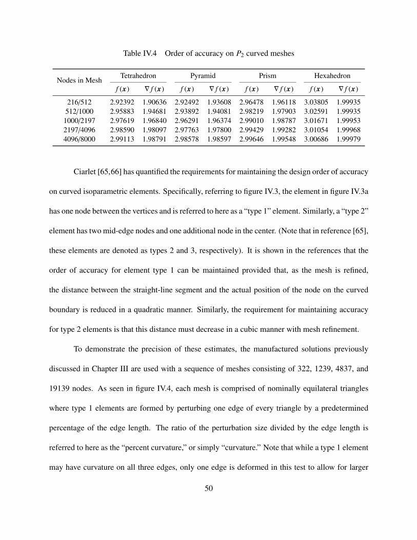
Table IV.4 Order of accuracy on P2 curved meshes



216/512 2.92392 1.90636 2.92492 1.93608 2.96478 1.96118 3.03805 1.99935512/1000 2.95883 1.94681 2.93892 1.94081 2.98219 1.97903 3.02591 1.999351000/2197 2.97619 1.96840 2.96291 1.96374 2.99010 1.98787 3.01671 1.999532197/4096 2.98590 1.98097 2.97763 1.97800 2.99429 1.99282 3.01054 1.999684096/8000 2.99113 1.98791 2.98578 1.98597 2.99646 1.99548 3.00686 1.99979

Ciarlet [65,66] has quantified the requirements for maintaining the design order of accuracy

on curved isoparametric elements. Specifically, referring to figure IV.3, the element in figure IV.3a

has one node between the vertices and is referred to here as a “type 1” element. Similarly, a “type 2”

element has two mid-edge nodes and one additional node in the center. (Note that in reference [65],

these elements are denoted as types 2 and 3, respectively). It is shown in the references that the

order of accuracy for element type 1 can be maintained provided that, as the mesh is refined,

the distance between the straight-line segment and the actual position of the node on the curved

boundary is reduced in a quadratic manner. Similarly, the requirement for maintaining accuracy

for type 2 elements is that this distance must decrease in a cubic manner with mesh refinement.

To demonstrate the precision of these estimates, the manufactured solutions previously

discussed in Chapter III are used with a sequence of meshes consisting of 322, 1239, 4837, and

19139 nodes. As seen in figure IV.4, each mesh is comprised of nominally equilateral triangles

where type 1 elements are formed by perturbing one edge of every triangle by a predetermined

percentage of the edge length. The ratio of the perturbation size divided by the edge length is

referred to here as the “percent curvature,” or simply “curvature.” Note that while a type 1 element

may have curvature on all three edges, only one edge is deformed in this test to allow for larger

50

d

(a) Element type 1

da

db

(b) Element type 2 (S-bend)

da

db

(c) Element type 2 (H-bend)

Figure IV.3 Elements for higher-order accuracy

deformations. Note also that if the percent curvature is held constant during mesh refinement, the

distance between the node at the mid-point of the straight-line segment and the actual position on

the edge only varies linearly. Quadric and cubic variations are obtained by dividing the percent

curvature by two and four, respectively, as the mesh is refined.

Figure IV.4 Grid Convergence on Meshes with Curved Elements

51

The solution variables are represented using nominally quadratic (P2) and cubic (P3) ele-

ments and the order of accuracy of each scheme is established and provided in Table IV.5. Here,

the first column provides the number of nodes present in the two meshes used in determining the

order of accuracy. The next two columns indicate the experimentally obtained order of accuracy

when the distance is reduced linearly with mesh refinement, while the final two columns indicate

results for a quadratic variation. As seen in the table, the design orders of accuracy are not ob-

tained when the distance is reduced linearly, whereas a quadratic variation yields the desired order.

It is important to note that while the analysis in reference [65] pertains to isoparametric elements,

the results obtained using cubic elements in this experiment actually correspond to subparametric

elements, but that the design order of accuracy is still maintained.

Table IV.5 Order of accuracy for type 1 elements

Nodes in MeshVariation with order h Variation with order h2

P2 P3 P2 P3

322/1,239 1.96 2.54 2.99 4.351,239/4,837 1.91 2.18 2.94 4.16

4,837/19,139 2.01 2.16 2.96 4.13

Similar results are shown in Table IV.6 for a series of elements of type 2, using cubic basis

functions. In the table, an “S-bend” refers to an element similar to that shown in figure IV.3b,

which is constructed by perturbing one node on the edge by a specified amount in the direction

of a “left-facing” normal, whereas the other node is perturbed in the opposite direction. Shown in

figure IV.3c, an “H-bend,” which also forms a type 2 element, is constructed by perturbing both

52

nodes in the same direction but with different amplitudes. As with the results shown previously

in Table IV.5, the results in Table IV.6 demonstrate that the design order of accuracy is obtained

by satisfying the requirements for reducing the distance between the straight-line segment and the

actual node locations. In contrast, violating these conditions yields suboptimal orders of accuracy.

Table IV.6 Order of accuracy for type 2 elements

Nodes in MeshVariation with order h2 Variation with order h3

S-bend H-bend S-bend H-bend

322/1,239 3.28 3.37 4.25 4.301,239/4,837 3.18 3.21 4.20 4.27

4,837/19,139 3.13 3.14 4.14 4.19

For a viscous flow, elements near the surface will often need to be curved to accommo-

date proper representation of the geometry without creating elements with negative areas/volumes.

However, the results presented in Tables IV.5 and IV.6 clearly indicate that strict requirements must

be met regarding the deformation of any element and, in particular, how the deformations must be

reduced as the mesh is refined. It is important to note that in practice, surface perturbations are

naturally decreased in a quadratic manner as the mesh is refined, thereby satisfying the require-

ments for type 1 elements. Unfortunately, while the results in Table IV.5 indicate that design order

can inherently be achieved with these elements, the desired order of accuracy may be difficult to

achieve for elements of type 2.

To examine this further, the method of manufactured solutions is again used on a series

of meshes to determine the order of accuracy. In the tests that follow, highly stretched elements

53

are present near one of the boundaries, although an inviscid flow is assumed to eliminate any

potential influence caused by the scaling of the stabilization matrix, or changes to other parameters

such as the Reynolds number. The geometry considered is shown in figure IV.5a, where parabolas

represent the upper and lower walls so that quadratic functions can precisely describe the geometry.

To avoid crossing grid lines when only “snapping” surface points, the grid along the upper wall

has normal spacing similar to that of an inviscid flow, whereas the lower wall has viscous-type

spacing. The x-coordinate spans from −0.5 to +0.5 with normal spacing along the lower wall of

5.0 × 10−4.

(a) Parabolic mesh (coarsest in series) (b) y-displacements

Figure IV.5 Mesh and contours of y-displacement for parabolic mesh

As output by a typical mesh generation procedure, the vertices at the endpoints of surface

edges are accurately positioned, whereas nodes in the middle of these edges require repositioning.

The location of these nodes is altered in the direction normal to the edges until the actual surface

intersection is found. These surface perturbations are subsequently propagated into the interior

using the methodology described in Chapter II. Figure IV.5b shows contours of the displacements

in the y-coordinate direction distributed throughout the mesh as a result of perturbing these points.

54

As seen, the largest y-displacements occur at the center of the mesh, decreasing at either end. Al-

though not shown, displacements in the x-direction vary differently, with the largest deformations

occurring toward the ends. For the sequence of grids consisting of 738, 2310, 8045, and 29760

nodes, the corresponding maximum perturbations at the surface are approximately 3.8 × 10−4,

9.88 × 10−5, 2.5 × 10−5, and 6.25 × 10−6, respectively. Note that the perturbations are reduced by

a factor of four with each mesh refinement, which also corresponds to a reduction in the percent

curvature by a factor of 2. The realized reductions in perturbation size thereby satisfy the quadratic

behavior necessary for a type 1 element, but are not reduced rapidly enough for an element of type

2.

Observed orders of accuracy for the manufactured solutions on these parabolic meshes are

given in Table IV.7. The table demonstrates that for linear and quadratic elements the theoretical

order of accuracy is obtained whereas suboptimal convergence is achieved for cubic elements.

Note that for linear elements, no repositioning of any nodes is required. Further, because quadratic

elements are of type 1, the naturally occurring squared reduction of the perturbations at the surface

allows the desired order to be maintained. In contrast, for cubic elements, the theoretical order

of accuracy is not achieved because the perturbations at the wall, which are propagated into the

interior, are only decreased in a quadratic manner as the mesh is refined instead of with a cubic

reduction as required. If the edges are “re-lofted” by fitting a quadratic through the nodes, the

resulting mesh is now comprised of type 1 elements. As seen in the fifth column of the table,

the design order of accuracy is again achieved. While the procedure used here for re-lofting the

nodes along the edge is not very general, the result again demonstrates that the design order can be

achieved by using subparametric type 1 elements. Also, it is relatively simple to modify the mesh

55

curving algorithm so that the displacements of nodes in the interior of the mesh always yields type

1 elements. Finally, as shown in the last column, if only surface nodes are “snapped” to the actual

geometry, the mapping of the interior elements from the reference space to the physical space

remains linear and the design order of accuracy is also obtained. It should be noted that, while

the P3 solution with type 2 elements failed to achieve the theoretical order of accuracy, the errors

observed are roughly one order of magnitude lower than for the P2 solution.

Table IV.7 Order of accuracy study for parabolic mesh with viscous wall spacing

Nodes in Mesh P1 P2 P3P3 P3

(re-lofting) (surface)

738/2,310 2.51 3.46 3.63 5.35 5.442,310/8,045 2.20 3.08 3.35 4.45 4.50

8,045/29,760 2.14 3.04 3.16 4.84 4.75

The results presented above demonstrate that achieving higher than third-order accuracy

for viscous flows requires some care when curving elements near the boundary. In particular,

while type 1 elements may be used to represent the geometry in conjunction with higher-order

polynomials for flow variables, the creation of type 2 elements needs to be minimized or avoided.

However, in perturbing the interior mesh points to accommodate changes at the surface, it is easily

seen how elements of type 2 can be created from elements with originally straight sides. First,

because the two vertices at the ends of each surface edge are typically placed correctly by the

grid generation procedure, any repositioning of mid-edge nodes naturally creates an oscillatory

behavior for the perturbations that are subsequently propagated into the interior. Secondly, as seen

in figure IV.6, even if elements of type 1 can accurately represent the surface, coarser elements

56

in the interior that may span surface undulations may be deformed into type 2 elements, which

could potentially impact the order of accuracy of the scheme. It is therefore recommended that

propagating surface perturbations into the interior be minimized as much as possible or that type 1

elements be used.

surface edges

interior edge

Figure IV.6 Creation of type 2 cells in the interior of the mesh

57

CHAPTER V

NUMERICAL RESULTS

Two Dimensions

Laminar Flow Over NACA 0012

The first demonstration case is for laminar flow over a NACA 0012 airfoil at a Mach num-

ber of 0.5, an angle of attack of 3 degrees, and a Reynolds number of 5000 based on the chord

of the airfoil. A depiction of the flow field is shown in figure V.1, which shows Mach number

contours computed using both linear elements and quadratic elements, on a mesh with 31,042

nodes. As seen in the figure, the wake captured using quadratic elements is less diffused and prop-

agates intact much farther downstream than the wake obtained using linear elements. Although

not quantitatively apparent from the figure, the flow also separates at approximately mid-chord of

the airfoil.

Computations are conducted using three meshes consisting of 3296, 9594, and 31042

nodes, respectively. Figure V.2a shows pressure coefficients computed using linear and quadratic

elements on the finest mesh, quadratic and cubic elements on the medium mesh, and cubic el-

ements on coarsest mesh. As seen, all the pressure distributions agree very well. Skin friction

coefficients, shown in figure V.2b also agree well between the schemes on different meshes, al-

though some differences are apparent near the leading edge. By examining the skin friction over

the first quarter of the airfoil (figure V.2c) it is seen that the solution obtained with linear elements

58

(a) P1 elements (b) P2 elements

Figure V.1 Mach contours for NACA 0012, M∞ = 0.5, α = 3, Re = 5000

clearly differs from the other solutions, which are all in excellent agreement with one another. Note

that in figure V.2c the solutions obtained with cubic elements have been depicted using symbols to

help discriminate between the other solutions. While further refinement is necessary to ensure that

the skin frictions do not exhibit further change, it is apparent that the solutions obtained with cubic

elements on the coarsest mesh, and quadratic elements on the medium mesh, are both somewhat

more accurate than the solution obtained with linear elements on the finest mesh.

It is interesting to compare the computer resources required in obtaining the solution with

quadratic elements on the medium mesh, cubic elements on the coarsest mesh, and linear elements

on the finest mesh. To facilitate the comparison, Table V.1 provides detailed statistics for each

mesh. Note that quadratic elements require additional degrees of freedom corresponding to the

number of edges in the mesh, whereas for cubic elements, two unknowns are added for each edge,

along with a subsequent unknown placed in the interior of the triangle. Because of the extra degrees

of freedom required for quadratic elements over linear elements, the total number of unknowns in

59

-0.6

-0.4

-0.2

0

0.2

0.4

0.6

0.8

1

1.20 0.2 0.4 0.6 0.8 1

Cp

x

Fine Mesh (P1)Fine Mesh (P2)

Medium Mesh (P2)Medium Mesh (P3)

Coarse Mesh (P3)

(a) Pressure coefficient over airfoil

-0.020

0.020.040.060.08

0.10.120.140.160.18

0 0.2 0.4 0.6 0.8 1

Cf

x



Coarse Mesh (P3)

(b) Skin friction coefficient over airfoil

-0.020

0.020.040.060.080.1

0.120.140.160.18

0 0.05 0.1 0.15 0.2 0.25

Cf

x



Coarse Mesh (P3)

(c) Skin friction coefficient near leading edge

Figure V.2 Results for laminar flow over NACA 0012 airfoil: M∞ = 0.5, α = 3, Re = 5000

60

the medium mesh is approximately 20% greater (38,054) than in the finest mesh with linear ele-

ments. For cubic elements on the coarsest mesh there are about 6% fewer (29,181) unknowns than

for the finest mesh with linear elements. The work required to compute residuals is proportional

to the number of triangles multiplied by the number of Gauss points used in each triangle. Us-

ing Table V.1 and assuming 3 Gauss points for linear elements, 7 for quadratic elements, and 12

for cubic elements, it is easily estimated that the residual computation for quadratic elements re-

quires only about 70% of the work needed for linear elements whereas cubic elements only require

roughly 40% of the work needed for linear elements. Further reductions can be achieved using 6

Gauss points for quadratic elements and 11 points for cubic elements without adversely effecting

accuracy. For an explicit scheme, this would imply that significant savings are available by using

higher-order elements. However, in the present implementation, a higher percentage of time is

spent in assembling and solving the linear system so that the cost between the schemes is roughly

equivalent. It is important to note several key points. First, while the computer resources required

for obtaining the solution with linear elements on the finest mesh is similar to that required for the

higher-order schemes on coarser meshes, the solution obtained with linear elements is clearly not

as accurate as the other solutions. Further refinement is required for the linear elements to accu-

rately assess the relative timings. Secondly, in this example there is no exact solution and therefore

no precise measure of the errors so the comparisons are only qualitative. Finally, it should be

noted that to achieve equal accuracy between linear and quadratic elements, the mesh spacing for

the quadratic elements is larger and varies as the mesh spacing for linear elements raised to the 2/3

power (hp2 ≈ h2/3p1 ). Similarly, for cubic elements the mesh spacing required to achieve a specified

61

level of error varies as the square root of the mesh spacing for linear elements (hp3 ≈ h1/2p1 ). Be-

cause of these nonlinear relationships, the relative savings depends on the level of error desired in

the computations, with the largest savings occurring for lower errors.

Table V.1 Mesh statistics for NACA 0012

Fine Mesh Medium Mesh Coarse Mesh

Nodes 31,042 9,594 3,296Edges 92,482 28,460 9,727

Triangles 61,440 18,866 6,431

As noted in Chapter II, the stabilization matrices can be designed using flux formulas orig-

inally developed for finite-volume schemes. Figure V.3 depicts skin friction results obtained using

the “standard” stabilization matrix given in equation (II.18), as well as skin frictions computed

using stabilization matrices based on van Leer’s flux-vector splitting [42, 43]. In figure V.3a, skin-

friction results computed with linear elements are shown along the upper surface of the airfoil for

all three meshes described above. It is seen that the skin friction changes as the mesh is refined,

although the agreement between the results obtained with the different stabilization matrices is

very good and indicates no significant difference in the level of dissipation. In contrast, seen in

figure V.3b, similar results obtained with a finite-volume scheme exhibit significant differences,

with the flux-vector splitting results being clearly more dissipative than those obtained with flux-

difference splitting. For the finite-volume scheme, less dissipation is present for flux-difference

splitting because of a vanishing eigenvalue corresponding to the velocity normal to the wall [68].

62

In contrast, for the Petrov-Galerkin scheme, the dissipation is proportional to the inverse of the

flux Jacobian so one would not expect higher dissipation with flux-vector splitting.

-0.020

0.020.040.060.08

0.10.120.140.160.18

0 0.05 0.1 0.15 0.2 0.25

Cf

x

Baseline τ Fine MeshFVS-τ Fine Mesh

Baseline τ Medium MeshFVS-τ Medium Mesh

Baseline τ Coarse MeshFVS-τ Coarse Mesh

(a) Skin friction coefficients computed with stabiliza-tion matrices based on flux-difference and flux-vector splitting

-0.020

0.020.040.060.080.1

0.120.140.160.18

0 0.05 0.1 0.15 0.2 0.25

Cf

x

FDS Fine MeshFVS Fine Mesh

FDS Medium MeshFVS Medium Mesh

FDS Coarse MeshFVS Coarse Mesh

(b) Skin friction coefficients computed using a finite-volume scheme with both flux-difference splittingand flux-vector splitting

Figure V.3 Effect of stabilization matrices on skin friction coefficient

Inviscid Flow Over NACA 0012

The next case is for subsonic inviscid flow over a NACA 0012 airfoil at a free-stream

Mach number of 0.5 and an angle of attack of two degrees. The intent of presenting this case

is to simply demonstrate another potential advantage to considering alternate formulations of the

stabilization matrix. Here, the formulation for the stabilization matrix is based on the flux-vector

splitting formulas given by Hänel [69], which are modifications to van Leer’s original splittings

so that total enthalpy can be maintained throughout the flow-field. Figures V.4a and V.4b show

the pressure distribution and total enthalpy errors, respectively, along the surface of the airfoil. As

seen in figure V.4a, the pressure distributions obtained using the new stabilization matrix agrees

63

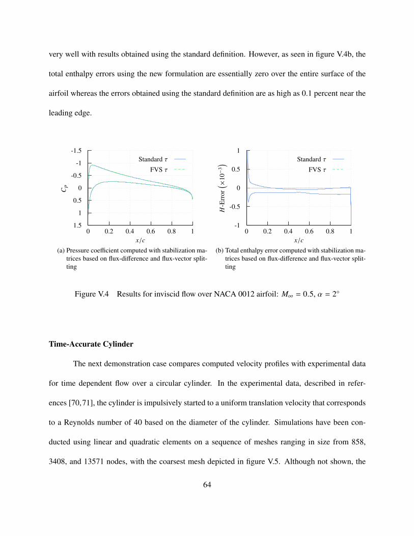
very well with results obtained using the standard definition. However, as seen in figure V.4b, the

total enthalpy errors using the new formulation are essentially zero over the entire surface of the

airfoil whereas the errors obtained using the standard definition are as high as 0.1 percent near the

leading edge.

-1.5

-1

-0.5

0

0.5

1

1.50 0.2 0.4 0.6 0.8 1

Cp

x/c

Standard τ

FVS τ

(a) Pressure coefficient computed with stabilization ma-trices based on flux-difference and flux-vector split-ting

-1

-0.5

0

0.5

1

0 0.2 0.4 0.6 0.8 1H

-Err

or( ×

10−3

)

x/c

Standard τ

FVS τ

(b) Total enthalpy error computed with stabilization ma-trices based on flux-difference and flux-vector split-ting

Figure V.4 Results for inviscid flow over NACA 0012 airfoil: M∞ = 0.5, α = 2

Time-Accurate Cylinder

The next demonstration case compares computed velocity profiles with experimental data

for time dependent flow over a circular cylinder. In the experimental data, described in refer-

ences [70,71], the cylinder is impulsively started to a uniform translation velocity that corresponds

to a Reynolds number of 40 based on the diameter of the cylinder. Simulations have been con-

ducted using linear and quadratic elements on a sequence of meshes ranging in size from 858,

3408, and 13571 nodes, with the coarsest mesh depicted in figure V.5. Although not shown, the

64

finest mesh has 248 nodes around the circumference of the cylinder with normal spacing at the wall

of 0.007. Subsequent coarser meshes have approximately one-half and one-quarter of the number

of mesh points on the surface so that the coarsest mesh only has 62 points in this region. For all

the meshes, no clustering is provided along the wake centerline. Although the experimental data

corresponds to an incompressible flow, the current simulations are run at a free-stream Mach num-

ber of 0.2. All computations are done using second-order backward-time differencing with a time

step of 0.01, non-dimensionalized by the reference length and the free-stream speed of sound. It

should be noted that simulations have also been done using a time step of 0.05 with no observable

differences in the computed profiles.

(a) Coarsest Mesh for Circular Cylinder (b) Near-Field View of Mesh

Figure V.5 Mesh for Circular Cylinder

A depiction of the computed start-up process is shown in figure V.6, where contours of the

x-component of velocity are shown at non-dimensional times where experimental data exists [70,

65

71]. As seen in the figures, the flow at each time is symmetric, with the wake growing continuously

as time progresses.

(a) t = 2.7 (b) t = 3.7

(c) t = 5.3 (d) t = 10.5

Figure V.6 Contours of the x-component of velocity for impulsively started cylinder

Figure V.7 shows a comparison of the computationally obtained x-component of velocity

along the x-axis with those from the experiment. Results obtained using linear elements are shown

on the left side of the figure, whereas similar results are shown on the right side for quadratic ele-

ments. It is seen in the figures that for linear elements, the results on the coarsest mesh are in poor

agreement with experiment but continually improve as the mesh is refined until good agreement is

obtained on the finest mesh with 13,571 degrees of freedom. In contrast, for quadratic elements

good agreement is obtained on the coarsest mesh containing only 3,338 degrees of freedom. The

solutions on the two finer meshes are very similar to those on the coarsest mesh but are slightly

66

smoother aft of approximately two diameters downstream of the cylinder. Overall, the compar-

isons with experiment are very good and demonstrate that accurate solutions can be obtained using

the higher-order elements on a much coarser mesh than required for linear elements.

67

-0.2

0

0.2

0.4

0.6

0.8

1

0 1 2 3 4 5

u-V

eloc

ity

x (Measured from Cylinder Center)

2.7 (Comp)2.7 (Exp)3.7 (Comp)3.7 (Exp)5.3 (Comp)5.3 (Exp)10.5 (Comp)10.5 (Exp)

(a) Coarse mesh, linear elements

-0.2

0

0.2

0.4

0.6

0.8

1

0 1 2 3 4 5

u-V

eloc

ity



(b) Coarse mesh, quadratic elements

-0.2

0

0.2

0.4

0.6

0.8

1

0 1 2 3 4 5

u-V

eloc

ity



(c) Medium mesh, linear elements

-0.2

0

0.2

0.4

0.6

0.8

1

0 1 2 3 4 5

u-V

eloc

ity



(d) Medium mesh, quadratic elements

-0.2

0

0.2

0.4

0.6

0.8

1

0 1 2 3 4 5

u-V

eloc

ity



(e) Fine mesh, linear elements

-0.2

0

0.2

0.4

0.6

0.8

1

0 1 2 3 4 5

u-V

eloc

ity



(f) Fine mesh, quadratic elements

Figure V.7 Comparison of computed velocity profiles with experimental data

68

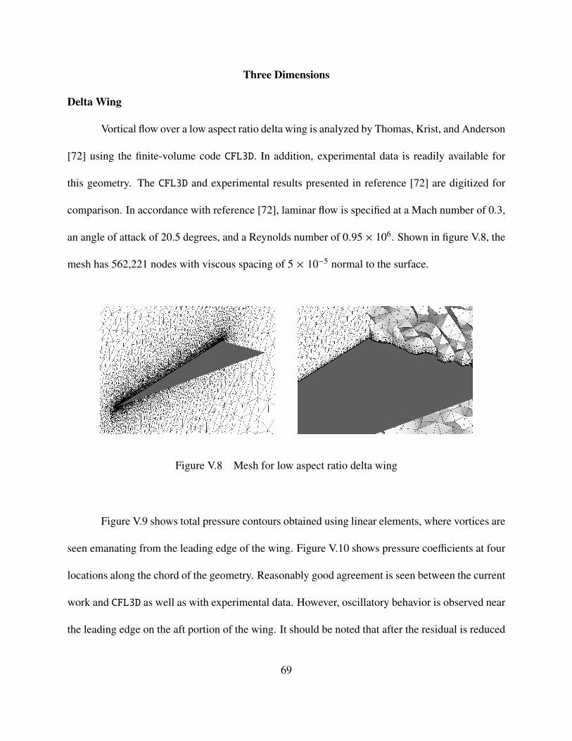
Three Dimensions

Delta Wing

Vortical flow over a low aspect ratio delta wing is analyzed by Thomas, Krist, and Anderson

[72] using the finite-volume code CFL3D. In addition, experimental data is readily available for

this geometry. The CFL3D and experimental results presented in reference [72] are digitized for

comparison. In accordance with reference [72], laminar flow is specified at a Mach number of 0.3,

an angle of attack of 20.5 degrees, and a Reynolds number of 0.95 × 106. Shown in figure V.8, the

mesh has 562,221 nodes with viscous spacing of 5 × 10−5 normal to the surface.

Figure V.8 Mesh for low aspect ratio delta wing

Figure V.9 shows total pressure contours obtained using linear elements, where vortices are

seen emanating from the leading edge of the wing. Figure V.10 shows pressure coefficients at four

locations along the chord of the geometry. Reasonably good agreement is seen between the current

work and CFL3D as well as with experimental data. However, oscillatory behavior is observed near

the leading edge on the aft portion of the wing. It should be noted that after the residual is reduced

69

to about 2 × 10−9, unsteadiness in the solution is observed and reduction of the residual no longer

occurs.

Figure V.9 Contours of total pressure

Results have also been obtained for the delta wing configuration using quadratic elements.

For these simulations, a mesh with 200,918 nodes has been generated, with spacing at the wall

three times larger than on the previous mesh and fewer triangles on the surface. The resulting

pressure distributions are shown in figure V.11, where it is observed that generally good agreement

is obtained with experimental data and with the results of reference [72]. As with the results

obtained with linear elements, the solution near the leading edge exhibits some oscillations.

70

-0.4-0.2

00.20.40.60.8

11.21.41.6

0 0.2 0.4 0.6 0.8 1

−Cp

Semispan

Current WorkCFL3DExperiment

(a) x/L = 0.3

-0.4-0.2

00.20.40.60.8

11.21.4

0 0.2 0.4 0.6 0.8 1−C

p

Semispan


(b) x/L = 0.5

-0.4-0.2

00.20.40.60.8

11.2

0 0.2 0.4 0.6 0.8 1

−Cp

Semispan


(c) x/L = 0.7

-0.2-0.1

00.10.20.30.40.50.60.7

0 0.2 0.4 0.6 0.8 1

−Cp

Semispan


(d) x/L = 0.9

Figure V.10 Cp plots at various stations along delta wing, linear elements

71

-0.4-0.2

00.20.40.60.8

11.21.41.6

0 0.2 0.4 0.6 0.8 1

−Cp

Semispan


(a) x/L = 0.3

-0.4-0.2

00.20.40.60.8

11.21.4

0 0.2 0.4 0.6 0.8 1−C

p

Semispan


(b) x/L = 0.5

-0.4-0.2

00.20.40.60.8

11.2

0 0.2 0.4 0.6 0.8 1

−Cp

Semispan


(c) x/L = 0.7

-0.2-0.1

00.10.20.30.40.50.60.7

0 0.2 0.4 0.6 0.8 1

−Cp

Semispan


(d) x/L = 0.9

Figure V.11 Cp plots at various stations along delta wing, quadratic elements

72

Viscous flows over a three-dimensional circular cylinder

This test case considers three-dimensional viscous flow over a circular cylinder at a Reynolds

number of 2580 based on the diameter of the cylinder and free-stream Mach number of 0.2 [73].

The geometry definition and the computational mesh is displayed in figure V.12. The x-axis is

along the stream-wise flow direction and the z-axis is in the span-wise direction.

Figure V.12 Computational mesh (containing 68,629 tetrahedral elements) for the three-dimensional viscous flow over a circular cylinder

Flow-through boundary conditions are specified at the inlet and outlet. Periodic boundary

conditions are applied on the side walls in the span-wise direction while symmetry is imposed

for the top and bottom walls. The cylinder is modeled as a nonslip isothermal wall. The mesh

on the cylinder surface is represented by quadratic polynomials and the interior mesh points are

moved via the linear elasticity solver discussed in Chapter II to allow curved meshes in the viscous

boundary layer. Figure V.13 shows contours of the instantaneous stream-wise, transverse, and

73

span-wise velocities in the wake of the cylinder using the third-order scheme and second-order

backward difference time integration with a fixed time-step of 0.02. Unsteady recirculation is

clearly observed as are alternating regions of positive and negative transverse velocity.

(a) Instantaneous stream-wise velocity

(b) Instantaneous transverse velocity

(c) Instantaneous span-wise velocity

Figure V.13 Instantaneous velocities in the x-z plane (y=0) in the wake of the cylinder. 60contours are included from −0.2 to 0.2

Figure V.14 compares, with experimental data [73], various normalized quantities at several

stream locations in the wake region obtained with the third-order scheme. The current method

shows favorable agreement with the experimental results.

74

-5

-4

-3

-2

-1

0

1

2

-3 -2 -1 0 1 2 3

<u>/U

y/D

x/D = 0.7

x/D = 1

x/D = 1.5

x/D = 2

x/D = 2.5

x/D = 3

(a) Mean normalized stream-wise veloc-ity

-3

-2.5

-2

-1.5

-1

-0.5

0

0.5

-3 -2 -1 0 1 2 3

<v>/U

y/D

x/D = 0.7

x/D = 1

x/D = 1.5

x/D = 2

x/D = 2.5

x/D = 3

(b) Mean normalized transverse velocity

-3

-2.5

-2

-1.5

-1

-0.5

0

0.5

-3 -2 -1 0 1 2 3

<u′ u

′ >/U

2

y/D

x/D = 0.7

x/D = 1

x/D = 1.5

x/D = 2

x/D = 2.5

x/D = 3

(c) Normalized < u′u′ >

-2.4

-2

-1.6

-1.2

-0.8

-0.4

0

0.4

-3 -2 -1 0 1 2 3

<u′ v

′ >/U

2

y/D

x/D = 0.7

x/D = 1

x/D = 1.5

x/D = 2

x/D = 2.5

x/D = 3

(d) Normalized < u′v′ >

-3

-2.5

-2

-1.5

-1

-0.5

0

0.5

-3 -2 -1 0 1 2 3

<v′ v

′ >/U

2

y/D

x/D = 0.7

x/D = 1

x/D = 1.5

x/D = 2

x/D = 2.5

x/D = 3

(e) Normalized < v′v′ >

Figure V.14 Normalized quantities in the wake of the circular cylinder using 3rd order SUPG(dashed line) in comparison with experimental data (circles)

75

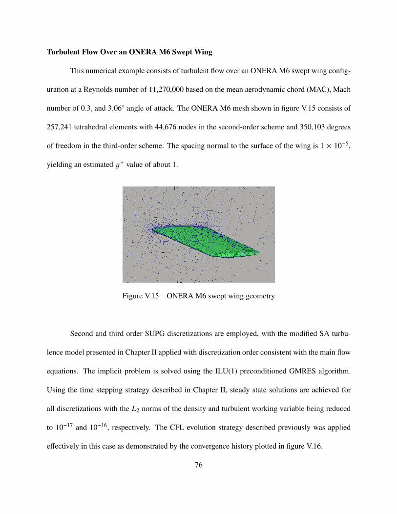
Turbulent Flow Over an ONERA M6 Swept Wing

This numerical example consists of turbulent flow over an ONERA M6 swept wing config-

uration at a Reynolds number of 11,270,000 based on the mean aerodynamic chord (MAC), Mach

number of 0.3, and 3.06 angle of attack. The ONERA M6 mesh shown in figure V.15 consists of

257,241 tetrahedral elements with 44,676 nodes in the second-order scheme and 350,103 degrees

of freedom in the third-order scheme. The spacing normal to the surface of the wing is 1 × 10−5,

yielding an estimated y+ value of about 1.

Figure V.15 ONERA M6 swept wing geometry

Second and third order SUPG discretizations are employed, with the modified SA turbu-

lence model presented in Chapter II applied with discretization order consistent with the main flow

equations. The implicit problem is solved using the ILU(1) preconditioned GMRES algorithm.

Using the time stepping strategy described in Chapter II, steady state solutions are achieved for

all discretizations with the L2 norms of the density and turbulent working variable being reduced

to 10−17 and 10−16, respectively. The CFL evolution strategy described previously was applied

effectively in this case as demonstrated by the convergence history plotted in figure V.16.

76

10−18

10−16

10−14

10−12

10−10

10−8

10−6

10−4

0 200 400 600 800 1000 1200 1400 1600

‖resi

dual‖ 2

iteration

ρuvwTν

Figure V.16 Convergence history for P2 SUPG solution on ONERA M6 swept wing geometry

The computed surface pressure coefficients obtained using the second- and third-order

SUPG discretizations are shown in figures V.17a and V.17b for various locations along the semi-

span. A CFL3D solution obtained from a substantially fine grid is shown to serve as a benchmark

solution . Both the P1 and P2 solutions show good agreement with the benchmark CFL3D results.

-1.5

-1

-0.5

0

0.5

10.1 0.2 0.3 0.4 0.5 0.6 0.7 0.8 0.9 1

Cp

x

20 44 65 80 90

(a) P1

-1.5

-1

-0.5

0

0.5

10.1 0.2 0.3 0.4 0.5 0.6 0.7 0.8 0.9 1

Cp

x

20 44 65 80 90

(b) P2

Figure V.17 Pressure coefficients plotted at various span-wise locations on the turbulent ONERAM6. Solid lines represent the CFL3D solution while dashed lines represent the SUPGsolutions. The span-wise locations (as % semi-span) are indicated above each curve

77

To demonstrate the importance of accurately representing curved meshes, figure V.18 shows

the pressure coefficients at 65% semi-span obtained using a piecewise linear geometry representa-

tion for the third order SUPG scheme. Although convergence was achieved to machine precision,

the linear geometry definition clearly has a negative impact on the accuracy of the obtained so-

lution. The non-smooth surface geometry causes significant oscillations to appear in the pressure

distribution. This further emphasizes the need for a robust strategy for obtaining curved higher-

order meshes.

−1.5

−1

−0.5

0

0.5

10.35 0.4 0.45 0.5 0.55 0.6 0.65 0.7 0.75 0.8 0.85 0.9

Cp

x

Figure V.18 Pressure coefficients at 65% semi-span for P2 solution on the linear mesh

Turbulent Flow over a NASA Trap Wing

Finally, results are shown below for turbulent flow over a NASA trap wing configuration

used in the 1stAIAA CFD High Lift Prediction Workshop [74]. In this paper, only configuration

one, without brackets, is considered with a Reynolds number of 4,300,000 based on the mean

aerodynamic chord (MAC), 12.99 angle of attack, and a Mach number of 0.2.

78

This test case was solved using the second and third order SUPG discretizations where the

mesh contains 1,126,835 tetrahedral elements with the 194,370 nodes in the second-order scheme

and 1,528,767 degrees of freedom in the third-order scheme. It should be noted that these meshes

are much coarser than those provided for the High Lift Prediction Workshop.1 Also, in contrast

to the ONERA M6 case, curving the mesh using linear elasticity did not result in any negative

Jacobians.

(a) Top view. (b) Bottom view.

Figure V.19 Surface mesh for trap wing geometry

1http://hiliftpw.larc.nasa.gov/index-workshop1.html

79

http://hiliftpw.larc.nasa.gov/index-workshop1.html

Contours of the computed turbulence working variable at three span-wise locations are

shown in figure V.20 for the third-order scheme. The maximum turbulence working variable ap-

pears in the circulation region between the slat and main wing, with significant values also occur-

ring in the circulation region between the main wing and the flap.

Figure V.20 Turbulence working variable at three stations along trap wing configuration

Figures V.21 to V.27 compare computed pressure coefficients with experimental wind tun-

nel data at various stations along the semi-span of the three elements. At all stations, the second-

order solution under-predicts the negative pressure on the upper surface of all three wing elements.

This under-prediction is most severe on the upper surface of the flap element whose discretization

is very coarse with only about 10 points along the upper surface. The third order solution shows

vast improvement in this regard. Both discretization orders suffer from oscillations in the pressure

distributions, especially near trailing edges. Again, the third order solution displays improvement

in this regard as well. However, both solutions exhibit oscillations in the pressure distribution

80

along the chord of the slat element; this is likely exacerbated by the coarseness of the mesh on that

element.

-3

-2

-1

0

17 8 9 10 11 12 13

Cp

x

(a) slat

-4

-3

-2

-1

0

1

25 10 15 20 25 30 35 40 45 50

x

PG P1PG P2

experiment

(b) main wing

-2.5-2

-1.5-1

-0.50

0.51

1.52

46 48 50 52 54 56 58 60 62

x

(c) flap

Figure V.21 Pressure coefficients at 17% semi-span on the NASA trap wing

-3

-2

-1

0

1

213 14 15 16 17

Cp

x

(a) slat

-5

-4

-3

-2

-1

0

1

215 20 25 30 35 40 45 50 55

x

PG P1PG P2

experiment

(b) main wing

-2.5-2

-1.5-1

-0.50

0.51

1.52

50 52 54 56 58 60 62 64

x

(c) flap


It should be noted that this case was run using the previous time-stepping strategy where the

CFL number was held constant until the residual for the turbulence model began to reduce. This

was done simply because the newer strategy had not yet been implemented. For the second-order

81

-4

-3

-2

-1

0

1

221 22 23 24 25 26 27

Cp

x

(a) slat

-5

-4

-3

-2

-1

0

1

220 25 30 35 40 45 50 55 60

x

PG P1PG P2

experiment

(b) main wing

-2.5-2

-1.5-1

-0.50

0.51

1.52

54 56 58 60 62 64 66 68

x

(c) flap


-4

-3

-2

-1

0

1

226 27 28 29 30

Cp

x

(a) slat

-5

-4

-3

-2

-1

0

1

225 30 35 40 45 50 55 60

x

PG P1PG P2

experiment

(b) main wing

-2.5-2

-1.5-1

-0.50

0.51

1.556 58 60 62 64 66 68 70

x

(c) flap


-4

-3

-2

-1

0

1

234 35 36 37 38 39 40 41

Cp

x

(a) slat

-6

-5

-4

-3

-2

-1

0

1

235 40 45 50 55 60 65

x

PG P1PG P2

experiment

(b) main wing

-2.5-2

-1.5-1

-0.50

0.51

1.562 64 66 68 70 72

x

(c) flap


82

-4

-3

-2

-1

0

1

237 38 39 40 41 42

Cp

x

(a) slat

-6

-5

-4

-3

-2

-1

0

1

240 45 50 55 60 65

x

PG P1PG P2

experiment

(b) main wing

-3-2.5

-2-1.5

-1-0.5

00.5

11.5

62 64 66 68 70 72 74

x

(c) flap


-5-4-3-2-1012

46 47 48 49 50 51 52

Cp

x

(a) slat

-5

-4

-3

-2

-1

0

1

245 50 55 60 65 70

x

PG P1PG P2

experiment

(b) main wing

-3-2.5

-2-1.5

-1-0.5

00.5

11.5

68 70 72 74 76 78

x

(c) flap


83

solution, convergence of the density and turbulence working variable were reduced to 10−15 and

10−14, respectively. However, for the third-order accurate solution, the density residual has been

reduced by four orders of magnitude whereas the residual for the turbulence working variable has

only been reduced by two orders of magnitude over its initial value. In this case, it has been found

helpful to start the solution at a lower Reynolds number to provide some extra damping.

84

CHAPTER VI

CONCLUSION

Summary

In this research, the viability of the streamline/upwind Petrov-Galerkin (SUPG) method for

obtaining high-order solutions to the compressible Navier-Stokes equations with a modified SA

turbulence model has been established. The SUPG discretization is presented as a practical high-

order alternative to more popular (but potentially more computationally expensive) discontinuous

Galerkin schemes. Using the method of manufactured solutions, the order of accuracy for inviscid

and viscous flow solutions has been verified up to fourth order for two-dimensional flow and up

to third order for three-dimensional flow. Alternate formulations for the stabilization matrix have

been presented using flux functions commonly used in finite-volume schemes. Here, stabilization

matrices based on flux-vector splitting as well as flux-difference splitting were shown to provide

similar results. For viscous flows, additional terms are added to the stabilization matrix that ensure

proper order of accuracy when the viscous terms become dominant at low Reynolds numbers.

The modified SA turbulence model requires that the distance to the viscous surface be

known throughout the mesh. In the context of high-order methods, it is important that this distance

reflect the true curved geometry. As such, an efficient method for calculating distances to a curved

85

surface was presented. An octree data structure was utilized to facilitate an efficient nearest neigh-

bor search, while an iterative approach was used to find the distance between a point in space and

a curved parametric surface.

The importance of curved surface meshes has been demonstrated, and strategies for pro-

ducing such meshes have been outlined. In two dimensions, analytic surface definitions were

used to accurately capture curved surface geometries, while the interior mesh was deformed us-

ing a straight-forward algebraic mesh smoothing approach. Due to the complexities of three-

dimensional geometry, a more robust approach was required. Here, a CAPRI interface was used

to project the surface mesh onto the CAD defined geometry. To avoid collapsed interior ele-

ments in anisotropic boundary layer regions, a linear elasticity solver was utilized to displace the

interior mesh. When dealing with curved isoparametric elements, analysis of polynomial basis

functions has shown that curved elements require additional degrees of freedom to achieve the

proper order characteristics. It was observed through numerical experimentation, however, that the

unrepresented terms in the polynomial expansion fall below truncation error for moderately curved

elements. Additionally, it was demonstrated that achieving greater than third order accuracy for

isoparametric curved elements requires that the curvature of interior elements decrease in a manner

not typically achieved in practical application. However, it was shown that subparametric elements

can be utilized to obtain the desired order.

Finally, numerical results were presented for several two and three dimensional test cases

consisting of both steady and unsteady flows and involving inviscid, laminar, and turbulent flow so-

lutions. The numerical results showed strong agreement with experimental data and/or benchmark

results.

86

Recommendations for Future Work

While the viability of the high-order SUPG scheme for compressible turbulent flows has

been established, opportunities for future work remain. As discussed in the introduction, the great-

est cost benefit over other high-order schemes occurs at moderate orders. This predicates the need

for adaptive p-refinement, where initial solutions will consist of low order elements exclusively and

discretization is increased on an element-by-element basis as required. In addition, some issues

regarding robustness need to be addressed. In particular, the procedure for generating curved three-

dimensional meshes about complex geometries proved inadequate in a minority of cases. In this

research, the problem was overcome by restricting the curvature of the surface mesh in problem

areas. Although this strategy proved effective, such limitations are undesirable and warrant fur-

ther research. Finally, failure to reach machine convergence in some steady-state cases indicates

a need for further study. A more robust time-marching strategy for high-order methods should be

explored.

87

REFERENCES

[1] Vatsa, V. N., Lockard, D. P., and Khorrami, M. R., “Application of FUN3D Solver for Aeroa-coustics Simulation of a Nose Landing Gear Configuration,” 17th AIAA/CEAS AeroacousticsConference, Portland, OR, June 2011, AIAA Paper 2011-2820.

[2] Cockburn, B., Hou, S., and Shu, C.-W., “The Runge-Kutta local projection discontinuousGalerkin finite element method for conservation laws IV: the multidimensional case,” Math-ematics of Computation, Vol. 54, No. 190, 1990, pp. 545–581.

[3] Bassi, F. and Rebay, S., “A High-Order Accurate Discontinuous Finite Element Method forthe Numerical Solution of the Compressible Navier-Stokes Equations,” Journal of Computa-tional Physics, Vol. 131, No. 2, 1997, pp. 267–279.

[4] Bassi, F. and Rebay, S., “High-Order Accurate Discontinuous Finite Element Solution of the2D Euler Equations,” Journal of Computational Physics, Vol. 138, No. 2, 1997, pp. 251–285.

[5] Darmofal, D. and Fidkowski, K., “Development of a Higher-Order Solver for AerodynamicApplications,” 42nd AIAA Aerospace Sciences Meeting and Exhibit, American Institute ofAeronautics and Astronautics, Reno, NV, USA, Jan. 2004, AIAA paper 2004-436.

[6] Fidkowski, K. J., Oliver, T. A., Lu, J., and Darmofal, D., “p-Multigrid solution of high-order Discontinuous Galerkin Discretizations of the Compressible Navier-Stokes equations,”J. Comput. Phys., Vol. 207, 2005, pp. 92–113.

[7] Nastase, C. R. and Mavriplis, D. J., “High-order discontinuous Galerkin methods using anhp-multigrid approach,” Journal of Computational Physics, Vol. 213, No. 1, 2006, pp. 330–357.

[8] Persson, P.-O. and Peraire, J., “An Efficient Low Memory Implicit DG Algorithm for TimeDependent Problems,” 44th AIAA Aerospace Sciences Meeting and Exhibit, American Insti-tute of Aeronautics and Astronautics, Reno, NV, USA, Jan. 2006, AIAA paper 2006-113.

[9] Persson, P.-O. and Peraire, J., “Sub-Cell Shock Capturing for Discontinuous Galerkin Meth-ods,” 44th AIAA Aerospace Sciences Meeting and Exhibit, American Institute of Aeronauticsand Astronautics, Reno, NV, USA, Jan. 2006, AIAA paper 2006-112.

[10] Fidkowski, K. J. and Darmofal, D., “A Triangular Cut-cell Adaptive Method for High-orderDiscretizations of the Compressible Navier-Stokes Equations,” J. Comput. Phys., Vol. 225,No. 2, 2007, pp. 1653–1672.

88

[11] Wang, L., Techniques for High-order Adaptive Discontinuous Galerkin Discretizations inFluid Dynamics, Ph.D. thesis, University of Wyoming, April 2009.

[12] Diosady, L. T. and Darmofal, D. L., “Preconditioning methods for discontinuous Galerkin so-lutions of the Navier-Stokes equations,” Journal of Computational Physics, Vol. 228, No. 11,2009, pp. 3917–3935.

[13] Mavriplis, D., Nastase, C., Shahbazi, K., Wang, L., and Burgess, N., “Progress in High-Order Discontinuous Galerkin Methods for Aerospace Applications,” 47th AIAA AerospaceSciences Meeting, American Institute of Aeronautics and Astronautics, Orlando, FL, USA,Jan. 2009, AIAA-2009-601.

[14] Dumbser, M., “Arbitrary high order PN PM schemes on unstructured meshes for the com-pressible Navier-Stokes equations,” Computers & Fluids, Vol. 39, No. 1, 2010, pp. 60–76.

[15] Burgess, N. and Mavriplis, D., “Robust Computation of Turbulent Flows Using a Discon-tinuous Galerkin Method,” 50th AIAA Aerospace Sciences Meeting including the New Hori-zons Forum and Aerospace Exposition, American Institute of Aeronautics and Astronautics,Nashville, TN, USA, Jan. 2012, AIAA Paper 2012-457.

[16] Venkatakrishnan, V., Allmaras, S. R., Kamenetskii, D. S., and Johnson, F. T., “Higher orderschemes for the compressible Navier-Stokes equations,” 16th AIAA Computational Fluid Dy-namics Conference, American Institute of Aeronautics and Astronautics, Orlando, FL, USA,June 2003, AIAA-2003-3987.

[17] Brooks, A. N. and Hughes, T. J. R., “Streamline Upwind/Petrov-Galerkin Formulations forConvection Dominated Flows with Particular Emphasis on the Incompressible Navier-StokesEquations,” Computer Methods in Applied Mechanics and Engineering, Vol. 32, No. 1–3,Sept. 1982, pp. 199–259.

[18] Hughes, T. and Tezduyar, T., “Finite element methods for first-order hyperbolic systems withparticular emphasis on the compressible euler equations,” Computer Methods in Applied Me-chanics and Engineering, Vol. 45, No. 1–3, 1984, pp. 217–284.

[19] Hughes, T. J. R., “Recent progress in the development and understanding of SUPG methodswith special reference to the compressible Euler and Navier-Stokes equations,” InternationalJournal for Numerical Methods in Fluids, Vol. 7, No. 11, 1987, pp. 1261–1275.

[20] Tezduyar, T., “Stabilized Finite Element Formulations for Incompressible Flow Computa-tions,” Vol. 28 of Advances in Applied Mechanics, Elsevier, 1991, pp. 1–44.

[21] Franca, L. P. and Frey, S. L., “Stabilized finite element methods: II. The incompress-ible Navier-Stokes equations,” Computer Methods in Applied Mechanics and Engineering,Vol. 99, No. 2–3, 1992, pp. 209–233.

89

[22] Beau, G. L., Ray, S., Aliabadi, S., and Tezduyar, T., “SUPG finite element computationof compressible flows with the entropy and conservation variables formulations,” ComputerMethods in Applied Mechanics and Engineering, Vol. 104, No. 3, 1993, pp. 397–422.

[23] Soulaïmani, A. and Fortin, M., “Finite element solution of compressible viscous flows usingconservative variables,” Computer Methods in Applied Mechanics and Engineering, Vol. 118,No. 3–4, 1994, pp. 319–350.

[24] Almeida, R. C. and Galeão, A. C., “An adaptive Petrov-Galerkin formulation for the com-pressible Euler and Navier-Stokes equations,” Computer Methods in Applied Mechanics andEngineering, Vol. 129, No. 1–2, 1996, pp. 157–176.

[25] Bonhaus, D. L., A Higher Order Accurate Finite Element Method for Viscous CompressibleFlows, Ph.D. thesis, Virginia Polytechnic Institute and State University, Nov. 1998.

[26] Wong, J. S., Darmofal, D. L., and Peraire, J., “The solution of the compressible Euler equa-tions at low Mach numbers using a stabilized finite element algorithm,” Computer Methodsin Applied Mechanics and Engineering, Vol. 190, No. 43–44, 2001, pp. 5719–5737.

[27] Bassi, F., Crivellini, A., Rebay, S., and Savini, M., “Discontinuous Galerkin solution of theReynolds-averaged Navier-Stokes and k-[omega] turbulence model equations,” Computers &

Fluids, Vol. 34, No. 4–5, 2005, pp. 507–540.

[28] Tezduyar, T. E. and Senga, M., “Stabilization and shock-capturing parameters in SUPG for-mulation of compressible flows,” Computer Methods in Applied Mechanics and Engineering,Vol. 195, No. 13–16, 2006, pp. 1621–1632, A Tribute to Thomas J.R. Hughes on the Occasionof his 60th Birthday.

[29] Kirk, B. S. and Carey, G. F., “Development and validation of a SUPG finite element schemefor the compressible Navier-Stokes equations using a modified inviscid flux discretization,”International Journal for Numerical Methods in Fluids, Vol. 57, No. 3, 2008, pp. 265–293.

[30] Yano, M. and Darmofal, D. L., “Massively Parallel Solver for the High-Order Galerkin LeastSquares Method,” 19th AIAA Computational Fluid Dynamics Conference, American Instituteof Aeronautics and Astronautics, San Antonio, TX, USA, June 2009, AIAA-2009-4135.

[31] Kirk, B. S., Bova, S. W., and Bond, R. B., “The Influence of Stabilization Parameters inthe SUPG Finite Element Method for Hypersonic Flows,” 48th AIAA Aerospace SciencesMeeting, American Institute of Aeronautics and Astronautics, Orlando, FL, USA, Jan. 2010,AIAA-2010-1183.

[32] Hughes, T. J., Scovazzi, G., and Tezduyar, T. E., “Stabilized Methods for CompressibleFlows,” Journal of Scientific Computing, Vol. 43, No. 3, 2010, pp. 343–368.

[33] Chalot, F. and Normand, P.-E., “Higher-Order Stabilized Finite Elements in an IndustrialNavier-Stokes Code,” ADIGMA — A European Initiative on the Development of Adaptive

90

Higher-Order Variational Methods for Aerospace Applications, edited by N. Kroll, H. Bieler,H. Deconinck, V. Couaillier, H. van der Ven, and K. Sørensen, Vol. 113 of Notes on NumericalFluid Mechanics and Multidisciplinary Design, chap. 11, Springer Berlin Heidelberg, 2010,pp. 145–165.

[34] Kirk, B. and Oliver, T., “Validation of SUPG Finite Element Simulations of Shock-wave/Turbulent Boundary Layer Interactions in Hypersonic Flows,” 51st AIAA AerospaceSciences Meeting including the New Horizons Forum and Aerospace Exposition, Ameri-can Institute of Aeronautics and Astronautics, Grapevine, TX, USA, Jan. 2013, AIAA paper2013-306.

[35] Erwin, J. T., Anderson, W. K., Kapadia, S., and Wang, L., “Three-Dimensional StabilizedFinite Elements for Compressible Navier-Stokes,” AIAA Journal, Vol. 51, No. 6, June 2013,pp. 1404–1419.

[36] Erwin, J. T., Anderson, W. K., Wang, L., and Kapadia, S., “High-Order Finite-ElementMethod for Three-Dimensional Turbulent Navier-Stokes,” 21st AIAA Computational FluidDynamics Conference, American Institute of Aeronautics and Astronautics, San Diego, CA,USA, June 2013, AIAA-2013-2571.

[37] Anderson, W. K., Wang, L., Kapadia, S., Tanis, C., and Hilbert, B., “Petrov-Galerkin andDiscontinuous-Galerkin Methods for Time-Domain and Frequency-Domain ElectromagneticSimulations,” J. Comput. Phys., Vol. 230, 2011, pp. 8360–8385.

[38] Glasby, R. S., Burgess, N. K., Anderson, W. K., Wang, L., Mavriplis, D. J., and Allmaras,S. R., “Comparison of SU/PG and DG Finite-Element Techniques for the CompressibleNavier-Stokes Equations on Anisotropic Unstructured Meshes,” 51st AIAA Aerospace Sci-ences Meeting Including the New Horizons Forum and Aerospace Exposition, American In-stitute of Aeronautics and Astronautics, Grapevine, TX, Jan. 2013, AIAA paper 2013-691.

[39] Moro, D., Nguyen, N.-C., and Peraire, J., “Navier-Stokes Solution Using HybridizableDiscontinuous Galerkin Methods,” 20th AIAA Computational Fluid Dynamics Conference,American Institute of Aeronautics and Astronautics, June 2011, AIAA-2011-3407.

[40] Solin, P., Segeth, K., and Dolezel, I., High-Order Finite Element Methods, Studies in Ad-vanced Mathematics, Chapman and Hall, 2003.

[41] Barth, T. J., “Numerical methods for gasdynamic systems on unstructured meshes,” An In-troduction to Recent Developments in Theory and Numerics for Conservation Laws, editedby D. Kroner, M. Ohlberger, and C. Rhode, Vol. 5, Springer, New York, NY, USA, 1998, pp.195–285.

[42] van Leer, B., “Flux-vector splitting for the Euler equations,” Eighth International Conferenceon Numerical Methods in Fluid Dynamics, edited by E. Krause, Vol. 170 of Lecture Notes inPhysics, Springer Berlin / Heidelberg, 1982, pp. 507–512.

91

[43] Anderson, W. K., Thomas, J. L., and van Leer, B., “Comparison of finite volume flux vectorsplittings for the Euler equations,” AIAA journal, Vol. 24, No. 9, Sept. 1986, pp. 1453–1460.

[44] Steger, J. L. and Warming, R. F., “Flux vector splitting of the inviscid gasdynamic equationswith application to finite-difference methods,” Journal of Computational Physics, Vol. 40,No. 2, 1981, pp. 263–293.

[45] Gressier, J., Villedieu, P., and Moschetta, J.-M., “Positivity of Flux Vector SplittingSchemes,” Journal of Computational Physics, Vol. 155, No. 1, 1999, pp. 199–220.

[46] Wang, C. and Liu, J., “Positivity property of second-order flux-splitting schemes for the com-pressible Euler equations,” Discrete and Continuous Dynamical Systems – Series B, Vol. 3,No. 2, May 2003, pp. 201–228.

[47] Shakib, F., Hughes, T. J., and Johan, Z., “A new finite element formulation for computationalfluid dynamics: X. The compressible Euler and Navier-Stokes equations,” Computer Methodsin Applied Mechanics and Engineering, Vol. 89, No. 1–3, 1991, pp. 141–219, Second WorldCongress on Computational Mechanics.

[48] Franca, L. P., Frey, S. L., and Hughes, T. J. R., “Stabilized finite element methods: I. Ap-plication to the advective-diffusive model,” Computer Methods in Applied Mechanics andEngineering, Vol. 95, No. 2, 1992, pp. 253–276.

[49] Fries, T.-P. and Matthies, H. G., “A Review of Petrov-Galerkin Stabilization Approaches andan Extension to Meshfree Methods,” Tech. Rep. Informatikbericht Nr.: 2004-01, Instituteof Scientific Computing, Technical University Braunschweig, Brunswick, Germany, March2004.

[50] Saad, Y. and Schultz, M. H., “GMRES: a generalized minimal residual algorithm for solvingnonsymmetric linear systems,” SIAM J. Sci. Stat. Comput., Vol. 7, No. 3, July 1986, pp. 856–869.

[51] Saad, Y., Iterative methods for sparse linear systems, Society for Industrial and AppliedMathematics, Philadelphia, PA, USA, 2nd ed., 2003.

[52] Gropp, W., Lusk, E., and Skjellum, A., Using MPI: Portable Parallel Programming with theMessage Passing Interface, MIT Press, Cambridge, MA, 1994.

[53] Karypis, G., “METIS, University of Minnesota, Department of Computer Science,”http://www-users.cs.umn.edu/ karypis/metis.

[54] Wang, L., Anderson, W. K., and Erwin, J. T., “Solutions of High-order Methods for Three-dimensional Compressible Viscous Flows,” 42nd AIAA Fluid Dynamics Conference and Ex-hibit, American Institute of Aeronautics and Astronautics, New Orleans, LA, USA, June2012, AIAA Paper 2012-2836.

92

[55] Wang, L., Anderson, W. K., Erwin, J. T., and Kapadia, S., “High-order Methods for Solutionsof Three-dimensional Turbulent Flows,” 51st AIAA Aerospace Sciences Meeting includingthe New Horizons Forum and Aerospace Exposition, American Institute of Aeronautics andAstronautics, Grapevine, TX, USA, Jan. 2013, AIAA Paper 2013-856.

[56] de Barros Ceze, M. A., A Robust hp-Adaptation Method for Discontinuous Galerkin Dis-cretizations Applied to Aerodynamic Flows, Ph.D. thesis, University of Michigan, 2013.

[57] Allen, C. B., “Parallel Flow-Solver and Mesh Motion Scheme for Forward Flight Rotor Sim-ulation,” 24th AIAA Applied Aerodynamics Conference, American Institute of Aeronauticsand Astronautics, San Fransisco, CA, USA, June 2006, AIAA-2006-3476.

[58] Brock, W., Burdyshaw, C., Karman, S., Betro, V., Hilbert, B., Anderson, K., and Haimes, R.,“Adjoint-Based Design Optimization Using CAD Parameterization Through CAPRI,” 50thAIAA Aerospace Sciences Meeting including the New Horizons Forum and Aerospace Expo-sition, American Institute of Aeronautics and Astronautics, Nashville, TN, USA, Jan. 2012,AIAA Paper 2012-968.

[59] Zienkiewicz, O. C., Taylor, R. L., and Zhu, J. Z., The Finite Element Method: Its Basis andFundamentals, Butterworth-Heinemann, 30 Corporate Drive, Suite 400, Burlington, MA,USA, 2005.

[60] Salari, K. and Knupp, P., “Code Verification by the Method of Manufactured Solutions,”Tech. Rep. SAND2000-1444, Sandia National Laboratories, Albuquerque, NM, USA, June2000.

[61] Lee, N.-S. and Bathe, K.-J., “Effects of element distortions on the performance of isopara-metric elements,” Numerical Methods in Engineering, Vol. 36, No. 20, 1993, pp. 3553–3576.

[62] McLeod, R., “Node Requirements for High-order Approximation over Curved Finite Ele-ments,” IMA Journal of Applied Mathematics, Vol. 17, No. 2, 1976, pp. 249–254.

[63] McLeod, R., “High Order Transformation Methods for Curved Finite Elements,” IMA Jour-nal of Applied Mathematics, Vol. 21, No. 4, 1978, pp. 419–428.

[64] Šolín, P., Segeth, K., and žel, I., Higher-order finite element methods, Vol. 1, CRC Press,Boca Raton, FL, USA, 2004.

[65] Ciarlet, P. G., The Finite Element Method for Elliptic Problems, Society for Industrial andApplied Mathematics, Philadelphia, PA, USA, 2nd ed., 2002.

[66] Ciarlet, P. G. and Raviart, P., “Interpolation theory over curved elements, with application tofinite element methods,” Computer Methods in Applied Mechanics and Engineering, Vol. 1,No. 2, 1972, pp. 217–249.

[67] Johnson, C., Numerical Solution of Partial Differential Equations by the Finite ElementMethod, Dover, New York, NY, USA, 2009.

93

[68] van Leer, B., Thomas, J. L., Roe, P. L., and Newsome, R. W., “A comparison of numericalflux formulas for the Euler and Navier-Stokes equations,” 8th AIAA Computational FluidDynamics Conference, American Institute of Aeronautics and Astronautics, Honolulu, HI,USA, June 1987, AIAA-1987-1104.

[69] Hänel, D., Schwane, R., and Seider, G., “On the accuracy of upwind schemes for the solu-tion of the Navier-Stokes equations,” 8th AIAA Computational Fluid Dynamics Conference,American Institute of Aeronautics and Astronautics, Honolulu, HI, USA, June 1987, pp. 42–46, AIAA-1987-1105.

[70] Coutanceau, M. and Bouard, R., “Experimental determination of the main features of theviscous flow in the wake of a circular cylinder in uniform translation. Part 1. Steady flow,”Journal of Fluid Mechanics, Vol. 79, No. 02, 1977, pp. 231–256.

[71] Coutanceau, M. and Bouard, R., “Experimental determination of the main features of theviscous flow in the wake of a circular cylinder in uniform translation. Part 2. Unsteady flow,”Journal of Fluid Mechanics, Vol. 79, No. 2, 1977, pp. 257–272.

[72] Thomas, J. L., Krist, S. T., and Anderson, W. K., “Navier-Stokes computations of vorticalflows over low-aspect-ratio wings,” AIAA journal, Vol. 28, No. 2, Feb. 1990, pp. 205–212.

[73] Mohammad, A. H. and Wang, Z., “Large Eddy Simulation of Flow Over a Cylinder UsingHigh-order Spectral Difference Method,” Advances in Applied Mathematics and Mechanics,Vol. 2, No. 4, 2011, pp. 451–466.

[74] Rumsey, C., Slotnick, J., Long, M., Stuever, R., and Wayman, T., “Summary of the FirstAIAA CFD High-Lift Prediction Workshop,” Journal of Aircraft, Vol. 48, No. 6, 2011,pp. 2068–2079.

94

VITA

Jon Taylor Erwin was born in July of 1983 in Little Rock, Arkansas, to Dennis and Evonna

Erwin. He attended elementary school in Malvern, Arkansas, before moving to Conway, Arkansas,

in 1995. There Taylor developed interest in and aptitude for mathematics and computer science.

He graduated with honors from Conway High School in 2001. Taylor earned a Bachelor of Sci-

ence degree in Mathematics, with a minor in Computer Science, from the University of Central

Arkansas in 2007. He continued his education at the University of Central Arkansas, serving as

a graduate teaching assistant while pursuing a Master of Science degree in Applied Mathematics.

Upon graduation in 2009, Taylor moved to Chattanooga, Tennessee, accepting a graduate research

assistantship at the University of Tennessee at Chattanooga SimCenter. Taylor graduated with a

Ph.D. in Computational Engineering in December of 2013.

95

stabilized finite elements for compressible turbulent ... · pdf fileii.4 curved mesh...

Documents