stabilityofsinusoidal…josh/documents/2006/holingreiss... · stability of sinusoidal responses 605...
TRANSCRIPT
INTERNATIONAL JOURNAL OF CIRCUIT THEORY AND APPLICATIONSInt. J. Circ. Theor. Appl. 2006; 34:593–605Published online 11 September 2006 in Wiley InterScience (www.interscience.wiley.com). DOI: 10.1002/cta.372
Stability of sinusoidal responses of marginally stable bandpasssigma delta modulators
Charlotte Yuk-Fan Ho1,‡, Bingo Wing-Kuen Ling2,∗,† and Joshua D. Reiss1,§
1Department of Electronic Engineering, Queen Mary, University of London, Mile End Road,London, E1 4NS, U.K.
2Department of Electronic Engineering, Division of Engineering, King’s College London, Strand,London, WC2R 2LS, U.K.
SUMMARY
In this paper, we analyse the stability of the sinusoidal responses of second-order interpolative marginallystable bandpass sigma delta modulators (SDMs) with the sum of the numerator and denominator poly-nomials equal to one and explore new results on the more general second-order interpolative marginallystable bandpass SDMs. These results can be further extended to the high-order interpolative marginallystable bandpass SDMs. Copyright q 2006 John Wiley & Sons, Ltd.
Received 24 May 2005; Revised 20 March 2006
KEY WORDS: interpolative marginally stable bandpass sigma delta modulators; resonance; sinusoidalresponses
1. INTRODUCTION
Since sigma delta modulators (SDMs) can perform analog-to-digital (A/D) conversion usingsimple, robust and inexpensive circuits, and can achieve very high signal-to-noise ratio (SNR)because of the noise shaping characteristics [1], SDMs are found in many industrial and consumerelectronic products. One of the advantages of employing bandpass SDMs over the lowpass SDMsis to reduce the sampling frequency by operating the SDMs on high frequency narrowband signals,so bandpass SDMs become more popular and have been investigated in the communications, signalprocessing and circuits and systems societies extensively [2–5].
∗Correspondence to: Bingo Wing-Kuen Ling, Department of Electronic Engineering, Division of Engineering, King’sCollege London, Strand, London, WC2R 2LS, U.K.
†E-mail: [email protected]‡E-mail: [email protected]§E-mail: [email protected]
Contract/grant sponsor: Queen Mary, University of London
Copyright q 2006 John Wiley & Sons, Ltd.

594 C. Y.-F. HO, B. W.-K. LING AND J. D. REISS
Since SDMs consist of a quantizer, which is a non-linear component, in the feedback loop, thedynamical behaviours of SDMs could be very complex even though the loop filters in the SDMsare as simple as second order, rational, strictly proper and causal filters with a unit delay in thenumerator [2–5]. It was found that the trajectory of second-order bandpass SDMs may exhibitone or more ellipses or elliptic fractal patterns confined within two trapezoids when zero or stepinputs are applied [2–5]. Although these results help for understanding the dynamical behavioursof second-order bandpass SDMs, bandpass inputs should be employed for the analysis becausebandpass SDMs shape away the noise from bandpass regions and operate at bandpass signals. Somesimulation results based on bandpass inputs have been performed in Reference [2]. In Reference[6], statistical properties of the error signals have been investigated, but the behaviours of theSDMs have not been discussed. In Reference [7], periodic behaviours of the output sequenceshave been discussed, but chaotic and divergent behaviours of the SDMs have not been explored.
In this paper, we start at studying the sinusoidal responses of the SDMs introduced in References[2–5], then we explore new results on the more general second-order interpolative marginally stablebandpass SDMs and extend these results to the high-order interpolative marginally stable bandpassSDMs. The outline of this paper is as follows. The notations are introduced in Section 2. Both theanalytical and simulation results are presented in Section 3. Finally, a conclusion is summarizedin Section 4.
2. NOTATIONS
Consider the second-order interpolative marginally stable bandpass SDMs introduced in [2–5].The transfer function of the loop filter of the SDMs is denoted as F(z) = (2 cos �z−1 − z−2)/(1−2 cos �z−1 + z−2), where � is the filter parameter depending on the sampling frequency and theoperating frequency of the SDMs. For this second-order marginally stable bandpass loop filter,� is also the natural frequency of the loop filter and the SDMs shape away the noise from thisfrequency. Denote the input of the SDMs and the output of the loop filter are, respectively, u(k)and y(k). Then the SDM can be described by the following state space equation [2–5]:
x(k + 1) =Ax(k) + B(u(k) − s(k)) for k � 0 (1)
y(k) =Cx(k) + D(u(k) − s(k)) for k � 0 (2)
where x(k)≡[x1(k) x2(k)]T ≡ [y(k − 2) y(k − 1)]T is the state vector of the SDMs and the statevariables are defined as the delay version of the output of the loop filter, u(k) ≡[u(k−2) u(k−1)]Tis a vector containing the past two consecutive points from the input signal u(k),
A≡[
0 1
−1 2 cos �
](3)
is the system matrix,
B≡[
0 0
−1 2 cos �
](4)
is the matrix associated with the input of the loop filter, C and D are the matrices associated withthe output of the loop filter. Since the state variables are chosen as the delay version of the output
Copyright q 2006 John Wiley & Sons, Ltd. Int. J. Circ. Theor. Appl. 2006; 34:593–605DOI: 10.1002/cta

STABILITY OF SINUSOIDAL RESPONSES 595
of the loop filter, C and D are the last row of matrices A and B, respectively, and
s(k) ≡[Q(x1(k)) Q(x2(k))]T for k � 0 (5)
is the quantized state vector, in which the superscript T denotes the transpose operator,
Q(y)≡{1 y � 0
−1 otherwise(6)
is a one bit quantizer and � ∈ (−�, �)\{0}. When � ∈ {−�, 0, �}, the system will become eitherlowpass or highpass SDMs, which are out of the scope of this paper because this paper onlyfocuses on the bandpass SDMs. Since s(k) consists of only four possible values: [1 1]T, [1 −1]T,[−1 − 1]T, and [−1 1]T, s(k) can be viewed as a symbolic sequence and symbolic dynamicalapproach is employed for the analysis of the SDMs.
In this paper, since we study the sinusoidal responses, the input signal u(k) is represented inthe form of u(k) = c sin(�k + �) + d for k � 0, where c, �, � and d are the amplitude, frequency,phase shift and DC offset of the input signals, respectively. Without loss of generality, we canassume that � �= 0. For �= 0, the input signal becomes a step signal and it is reduced to the zeroor step response case, which is equivalent to the case when c= 0 and d is equal to the DC levelof the input signal. Moreover, we only consider the case when the natural frequency of the loopfilter �, the input signal u(k) and the initial condition x(0) are real, that is, �, c, d, �, � ∈ � andx(0)∈ �2. As a result, y(k) is also real.
3. RESULTS
In this section, we first study the second-order interpolative marginally stable bandpass SDMs withsum of numerator and denominator polynomials equal to one. Then, we will extend the results tothe case when the sum of numerator and denominator polynomials not equal to one.
3.1. SDMs with sum of numerator and denominator polynomials equal to one
When the output of the loop filters is bounded and the output sequences are eventually periodicwith periodM starting at the time index kM0 , we can define the admissible set of eventually periodicoutput sequences �≡⋃M�1 �M for k � k0, where �M is the admissible set of eventually periodicoutput sequences with period M for k � kM0 and k0 = maxM�1 kM0 , in which M∈Z+. �M can berepresented as
�M ≡ {sM ≡ (s(kM0 ), s(kM0 + 1), . . . , s(kM0 + M − 1)) : s(kM0 + i)
= s(kM0 + i + pM) for i = 0, 1, . . . , M − 1 and p ∈ Z+}Define the discrete-time Fourier coefficients of the eventually periodic output sequences with periodM for k � kM0 as ap for p= 0, 1, . . . , M − 1, that is
ap ≡ 1
M
kM0 +M−1∑k=kM0
s(k)e− j2�pk/M for p = 0, 1, . . . , M − 1
Copyright q 2006 John Wiley & Sons, Ltd. Int. J. Circ. Theor. Appl. 2006; 34:593–605DOI: 10.1002/cta
596 C. Y.-F. HO, B. W.-K. LING AND J. D. REISS
Then, the following lemma characterizes the constraints on ap for p= 0, 1, . . . , M − 1:
Lemma 1If y(k) is bounded, the output sequences are eventually periodic with period M for k � kM0 ,|�| �= |�| and 2�p/M �= |�| for p= 0, 1, . . . , M −1, then ap for p= 0, 1, . . . , M −1 has to satisfythe following two constraints:
M−1∑p=0
apamod(q−p+M,M) ={1 q = 0
0 q = 1, 2, . . . , M − 1(7)
and
Q
(M−1∑p=0
ap f1(k, p) + f2(k)
)=
M−1∑p=0
apej2�pk/M for k � kM0 (8)
where
f1(k, p) = C8ej2�pk/M + C9 cos �k + C10 sin �k for p= 0, 1, . . . , M − 1 and k � kM0 (9)
f2(k) = (x1(0)−Q(x1(0)))(sin(k−1)�−2 cos � sin k�)+(x2(0)−Q(x2(0)))(2 cos � sin(k+1)�− sin k�)
sin �
+C1 + C2 cos(�k) + C3 + C2 cos�
sin�sin(�k) + C4 cos(�k) + C5 + C4 cos �
sin �sin(�k) (10)
for k � 0, and mod(�, M) represents the remainder of �/M , in which
C1 = d(2 cos � − 1)
2(1 − cos �)(11)
C2 = sin�Re{C6} + cos� Im{C6}sin�
(12)
C3 = −Im{C6}sin�
(13)
C4 = sin �Re{C7} + cos � Im{C7}sin �
(14)
C5 = −Im{C7}sin �
(15)
C6 = c(sin � + sin(� − �)e− j�)(2 cos � − e− j�)
4 sin
(� + �
2
)sin
(� − �
2
) (16)
C7 = d(1 − 2 cos� + e− j�) + c(e j� − 1)(sin � + sin(� − �)e− j�)
4 sin
(� + �
2
)sin
(� − �
2
)(1 − e− j�)
(17)
Copyright q 2006 John Wiley & Sons, Ltd. Int. J. Circ. Theor. Appl. 2006; 34:593–605DOI: 10.1002/cta

STABILITY OF SINUSOIDAL RESPONSES 597
C8 = e− j2�p/M − 2 cos �
4 sin
(�
2+ �p
M
)sin
(�
2− �p
M
) (18)
C9 = 1
2 j sin �
(e j�
1 − e j2�p/Me j�− e j�
1 − e j2�p/Me− j�
)(19)
C10 = 1
2 j sin �
(e− j ((�/2)−�)
1 − e j2�p/Me− j�− e j ((�/2)−�)
1 − e j2�p/Me+ j�
)(20)
Re{�} and Im{�} denote, respectively, the real and imaginary part of �.
ProofSince y(k) is bounded and the output sequences are eventually periodic with period M for k � kM0 ,the Fourier representation of the eventually periodic output sequences with period M for k � kM0exists. Since (Q(y(k)))2 = 1 for k � 0, Equation (7) has to be satisfied. Besides, since |�| �= |�|and 2�p/M �= |�| for p= 0, 1, . . . , M −1, then by computing the outputs of the loop filter due to,respectively, the zero input and without quantizer feedback, the zero initial condition and withoutquantizer feedback, and zero initial condition and zero input, Equation (8) has to be satisfied,where the coefficients in Equation (8) are obtained by grouping the terms correspondingly. Hence,this completes the proof. �
The importance of Lemma 1 is that it provides information to check whether a binary eventu-ally periodic sequence with period M for k � kM0 is an eventually periodic admissible sequencegenerating a bounded trajectory for the SDMs or not. For the absolute value of the input sinusoidalfrequency and that of the harmonics of the eventually periodic output sequence with period Mfor k � kM0 not equal to that of the natural frequency of the loop filter, if we cannot find an initialcondition x(0) and a starting time index kM0 such that Equations (7) and (8) are satisfied, then thetest sequence is not an eventually periodic admissible sequence generating a bounded trajectoryfor the SDMs.
Since the input signals are periodic, the output of the loop filter and the output sequencesare assumed to be bounded and eventually periodic with period M for k � kM0 , respectively, thespectrum of y(k) will consist of impulses. As a result, fixed points and limit cycles may occurbut fractal and irregular chaotic patterns would not exhibit on the phase portrait. Figure 1 showssome phase portraits of these SDMs. Although the output sequences are eventually periodic withperiod M for k � kM0 , there are many different patterns exhibiting on the phase portraits as shownin Figure 1.
In Lemma 1, we assume that both the absolute value of the input sinusoidal frequency and thatof the harmonics of the eventually periodic output sequences with period M for k � kM0 are notequal to the absolute value of the natural frequency of the loop filter. However, as the bandpassSDMs shape away the noise from the natural frequency of the loop filter, the input sinusoidalfrequency is usually equal to the natural frequency of the loop filter. This case will be discussedin the following lemma.
Copyright q 2006 John Wiley & Sons, Ltd. Int. J. Circ. Theor. Appl. 2006; 34:593–605DOI: 10.1002/cta

598 C. Y.-F. HO, B. W.-K. LING AND J. D. REISS
Figure 1. Phase portraits of second-order interpolative bandpass SDMs when the output sequences areeventually periodic with period M for k�kM0 .
Copyright q 2006 John Wiley & Sons, Ltd. Int. J. Circ. Theor. Appl. 2006; 34:593–605DOI: 10.1002/cta

STABILITY OF SINUSOIDAL RESPONSES 599
Lemma 2Suppose y(k) is bounded and the output sequences are eventually periodic with period M fork � kM0 . Let q be a positive rational number. |�| = |�| = q� if and only if ∃p∗ ∈ {0, 1, . . . , M − 1}such that p∗ = M |�|/2� and ap∗ = c/2e− j ((�/2)−�).
ProofSince the output sequences are eventually periodic with period M for k � kM0 and y(k) is bounded,the Fourier representation on the eventually periodic output sequences with period M for k � kM0exists. If ∃p∗ ∈ {0, 1, . . . , M − 1} such that p∗ = M |�|/2�, then there exists an impulse located atthe natural frequency of the loop filter on the spectrum of the output sequences. This sinusoidalcomponent may cause resonance effect and has to be cancelled by the input sinusoidal signalsbecause y(k) is bounded. Hence, the input signals have to contain a sinusoidal component locatedat the natural frequency of the loop filter and this proves that |�| = |�|. To prove |�| is a rationalmultiple of �, since p∗ = M |�|/2� and p∗ is an integer, the result follows directly. For the converse,when |�| = |�|, in order to cancel the resonance effect generated by the input sinusoidal component,the Fourier component of the output sequences should have a component located at the naturalfrequency of the loop filter with the value ap∗ = (c/2)e− j ((�/2)−�). This proves the converse andcompletes the whole proof. �
The importance of Lemma 2 is for the proof of Theorem 1 that is stated below. From Lemma 2,we see that, unlike linear systems, the trajectory of the non-linear SDMs does not necessarily divergeeven though the input sinusoidal frequency is equal to the natural frequency of the loop filter.
Figures 2(b), (d) and (a) show, respectively, the frequency spectrum of x1(k), the frequencyspectrum of y(k) and the phase portrait of the SDMs when u(k) = 0.05 sin(�k/2) for k � 0,� = �/2 and x(0)=[0.1 0.2]T, in which the red and black lines in Figures 2(b)–(d) represent,respectively, the frequency spectrum of the corresponding spectra and the magnitude response dueto the initial condition of the loop filter. It can be seen from Figure 2(a) that the trajectory isbounded. Figure 2(c) shows the frequency spectrum of s1(k). It can be seen from Figure 2(c) thats1(k) is eventually periodic and the SDM exhibits limit cycle behaviour. Since � = �/2, accordingto Lemma 2, we can conclude that there exists an impulse located at the natural frequency ofthe loop filter on the spectrum of eventually periodic output sequences, which is also the inputsinusoidal frequency, and the corresponding Fourier coefficient is (c/2)e− j ((�/2)−�), as shown inFigure 2(c).
Now we extend Lemma 2 to the cases when the output sequences are aperiodic.
Theorem 1If y(k) is bounded, then |�| = |�| if and only if there exists an impulse located at the naturalfrequency of the loop filter on the spectrum of output sequences. Furthermore, for bounded y(k)and |�| = |�|, s(k) is aperiodic if and only if � is not a rational multiple of �.
ProofThe proof is similar to that of Lemma 2, so it is omitted here. �
The importance of this theorem is to provide information to check whether there is an impulselocated at the natural frequency of the loop filter on the spectrum of the output sequences or not.When the output of the loop filter is bounded, the existence of an impulse located at the naturalfrequency of the loop filter on the spectrum of the output sequences of the SDMs is equivalent
Copyright q 2006 John Wiley & Sons, Ltd. Int. J. Circ. Theor. Appl. 2006; 34:593–605DOI: 10.1002/cta
600 C. Y.-F. HO, B. W.-K. LING AND J. D. REISS
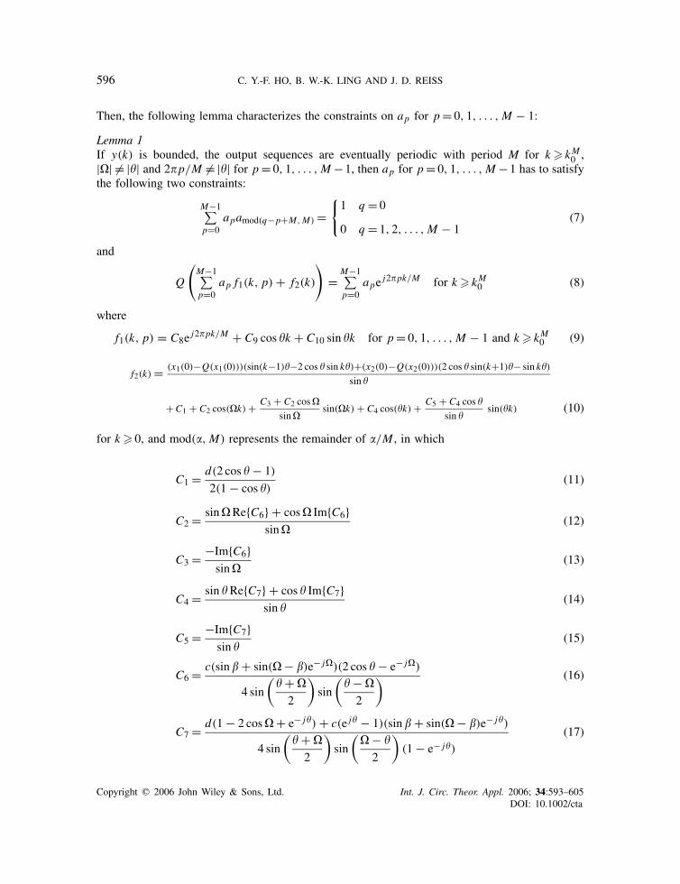
Figure 2. (a) Phase portrait of the second-order interpolative bandpass SDM; (b) frequency spectrum ofx1(k); (c) frequency spectrum of s1(k); and (d) frequency spectrum of y(k).
to the fact that the absolute value of the input sinusoidal frequency is equal to that of the naturalfrequency of the loop filter. Moreover, if y(k) is bounded and |�| = |�|, then the occurrence oflimit cycles is equivalent to the fact that the absolute value of the input sinusoidal frequency orthat of the natural frequency of the loop filter is a rational multiple of �. Based on these tworesults, it suggests that the absolute value of the input sinusoidal frequency, as well as that of thenatural frequency of the loop filter, should not be set at a rational multiple of � for avoiding theoccurrence of limit cycles.
If y(k) is bounded, |�| = |�| and � is not a rational multiple of �, then fractal or irregularchaotic patterns may be exhibited on the phase portrait. Figures 3(b) (d) and (a) show, respectively,the frequency spectrum of x1(k), the frequency spectrum of y(k) and the phase portrait of theSDM when u(k) = 0.1 sin(1.5k) for k � 0, � = 1.5 and x(0)= [0.1253 0.2877]T, in which thered and black lines in Figures 3(b)–(d) represent, respectively, the frequency spectrum of thecorresponding spectra and the magnitude response due to the initial condition of the loop filter.It can be seen from Figure 3(a) that the trajectory is bounded. According to Theorem 1, since|�| = |�|, we can conclude that there exists an impulse located at the natural frequency of theloop filter on the spectrum of output sequences, which is also the input sinusoidal frequency, as
Copyright q 2006 John Wiley & Sons, Ltd. Int. J. Circ. Theor. Appl. 2006; 34:593–605DOI: 10.1002/cta

STABILITY OF SINUSOIDAL RESPONSES 601
Figure 3. (a) Phase portrait of the second-order interpolative bandpass SDM; (b) frequency spectrum ofx1(k); (c) frequency spectrum of s1(k); and (d) frequency spectrum of y(k).
shown in Figure 3(c). In this example, since the natural frequency of the loop filter is 1.5, whichis not a rational multiple of �, so according to Theorem 1, s(k) is aperiodic. Figure 3(c) showsthe frequency spectrum of s1(k). It can be seen from Figure 3(c) that s1(k) is aperiodic and theSDM exhibits chaotic behaviour, as predicted by the theorem. Figure 4 shows another examplewhen u(k) = 0.01 sin(−1.746k) for k � 0, � = −1.8416 and x(0)=[0.01 0.01]T . In this case, thetrajectory is still bounded. Since |�| �= |�|, so according to Theorem 1, there does not exist animpulse located at the natural frequency of the loop filter on the spectrum of output sequences, asshown in Figure 4(c).
Next, we will explore the conditions when y(k) is unbounded.
Lemma 3Suppose that the output sequences are eventually periodic with period M for k � kM0 and |�| =|�| = q�, where q is a positive rational number. If ∀p∗ ∈ {0, 1, . . . , M−1}, ap∗ �= (c/2)e− j ((�/2)−�),then |y(k)| → +∞ for k → + ∞.
ProofThe proof follows directly from Lemma 2, so it is omitted here. �
Copyright q 2006 John Wiley & Sons, Ltd. Int. J. Circ. Theor. Appl. 2006; 34:593–605DOI: 10.1002/cta
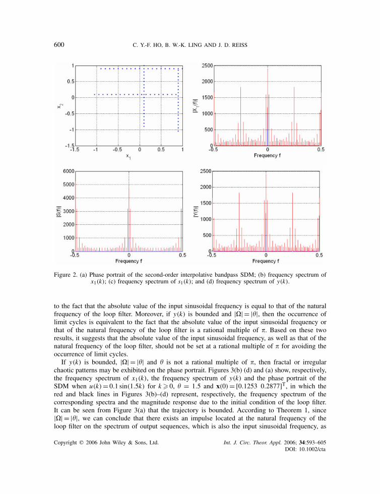
602 C. Y.-F. HO, B. W.-K. LING AND J. D. REISS
Figure 4. (a) Phase portrait of the second-order interpolative bandpass SDM; (b) frequency spectrum ofx1(k); (c) frequency spectrum of s1(k); and (d) frequency spectrum of y(k).
The importance of Lemma 3 is to provide information to check whether the output of the loopfilter diverges or not. It is worth noting that even though the output sequences are eventuallyperiodic with period M for k � kM0 , the resonance effect introduced by the input signals may notbe canceled by that of the eventually periodic output sequences when the corresponding Fouriercoefficient of the eventually periodic output sequences is not equal to (c/2)e− j ((�/2)−�). If thisis the case, then the output of the loop filter will diverge. Compared to the results reported inReference [5] that the second-order interpolative bandpass SDMs are globally stable for both zeroand step inputs no matter where the initial conditions are, the global stability for the sinusoidalresponse cases is not guaranteed.
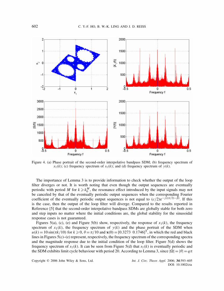
Figures 5(a), (c), (e) and Figure 5(b) show, respectively, the response of x1(k), the frequencyspectrum of x1(k), the frequency spectrum of y(k) and the phase portrait of the SDM whenu(k) = 10 sin(�k/10) for k � 0, � = �/10 and x(0)=[0.3273 0.1746]T, in which the red and blacklines in Figures 5(c)–(e) represent, respectively, the frequency spectrum of the corresponding spectraand the magnitude response due to the initial condition of the loop filter. Figure 5(d) shows thefrequency spectrum of s1(k). It can be seen from Figure 5(d) that s1(k) is eventually periodic andthe SDM exhibits limit cycle behaviour with period 20. According to Lemma 3, since |�| = |�| = q�
Copyright q 2006 John Wiley & Sons, Ltd. Int. J. Circ. Theor. Appl. 2006; 34:593–605DOI: 10.1002/cta

STABILITY OF SINUSOIDAL RESPONSES 603
Figure 5. (a) Response of x1(k); (b) phase portrait of the second-order interpolative bandpass SDM; (c)frequency spectrum of x1(k); (d) frequency spectrum of s1(k); and (e) frequency spectrum of y(k).
where q is a positive rational number, and ∀p∗ ∈ {0, 1, . . . , M − 1}ap∗ �= (c/2)e− j ((�/2)−�), we canconclude that the trajectory is unbounded, as shown in Figure 5(a) and (b).
3.2. SDMs with sum of numerator and denominator polynomials not equal to one
Now we extend the results to the case when the sum of the numerator and denominator polynomialsof the loop filter is not equal to one. That is, by denoting the loop filter of a second-order interpolativemarginally stable bandpass SDMs as F ′(z) = (�z−1 + �z−2)/(1− 2 cos �z−1 + z−2), where � and� are real and (�, �) �= (−2 cos �, 1).
Theorem 2If �>0, then ∃x(0) ∈ �2 such that |y(k)| → +∞ for k → +∞.
ProofThe proof is shown in Reference [8]. �
The importance of this theorem is to provide information to check whether the output of theloop filter diverges or not. If �>0, then the output of the loop filter may be unstable. Hence, it isimportant to choose the numerator coefficients such that ��0.
Copyright q 2006 John Wiley & Sons, Ltd. Int. J. Circ. Theor. Appl. 2006; 34:593–605DOI: 10.1002/cta

604 C. Y.-F. HO, B. W.-K. LING AND J. D. REISS
Figure 6. (a) Plot of x2(k) against x1(k); (b) frequency spectrum of x1(k); (c) frequency spectrum of s1(k);and (d) frequency spectrum of y(k).
3.3. High-order interpolative marginally stable bandpass SDMs
Although there are limits on the applications of second-order interpolative marginally stable band-pass SDMs, high-order ones are found many applications and part of the results in Theorem 1 isapplied for those high-order ones. If the absolute value of the input sinusoidal frequency is notequal to that of the natural frequencies of the loop filter and there is no impulse located at thenatural frequencies of the loop filter on the spectrum of the output sequences, then the outputof the loop filter is bounded. Figure 6 shows responses of 8 order interpolative marginally stablebandpass SDMs designed via the Matlab sigma-delta toolbox [9] with oversampling ratio 64 andcentre frequency �/2. It can be checked that the natural frequencies of the loop filter are e± j1.5497,e± j1.5625, e± j1.5791 and e± j1.5919. Assume that the input of the SDM is u(k) = 0.1 sin(�k/2)for k�0. Then the absolute value of the input sinusoidal frequency is not equal to that of thenatural frequencies of the loop filter. Figures 6(b), (d) and (a) show, respectively, the frequencyspectrum of x1(k), the frequency spectrum of y(k) and the plot of x2(k) against x1(k) under zeroinitial condition, in which the red and black lines in Figures 6(b)–(d) represent, respectively, thefrequency spectrum of the corresponding spectra and the natural frequencies of the loop filter. Itcan be seen from Figure 6(c) that there is no impulse located at the natural frequencies of the loop
Copyright q 2006 John Wiley & Sons, Ltd. Int. J. Circ. Theor. Appl. 2006; 34:593–605DOI: 10.1002/cta

STABILITY OF SINUSOIDAL RESPONSES 605
filter on the spectrum of the output sequences, so the trajectory is bounded. It can be seen fromFigure 6(a) that x1(k) is bounded and the trajectory is confirmed with certain region in the statespace.
4. CONCLUSION
Most of the existing stability analysis of SDMs is restricted to time domain analysis and stepresponses for lowpass systems. In this work, we have used frequency domain analysis to investigatethe stability of bandpass SDMs with respect to sinusoidal responses. The main contribution of thispaper is to study the admissibility conditions on the Fourier coefficients of the eventually periodicoutput sequences that generate bounded trajectories, and to analyse the stability of sinusoidalresponses of second-order interpolative bandpass SDMs in the frequency domain. In Lemma 1,we provided conditions as to whether an eventually periodic output sequence is an admissiblesequence for generating a bounded trajectory. From Lemma 2 we showed that the trajectory ofan SDM does not necessarily diverge even though the input sinusoidal frequency is equal to thenatural frequency of the loop filter. Theorem 1 then generalizes Lemma 2 to the aperiodic caseand provides information for the occurrence of fractal and chaotic behaviours. Finally, Lemma 3provided conditions for the divergent behaviour. These theoretical results were confirmed bysimulation on a variety of SDMs with different sinusoidal responses and can be further extendedto high-order interpolative bandpass SDMs. High-order bandpass SDMs are useful in many practicalsystems because the oversampling ratios of bandpass SDMs are usually lower than that of lowpassSDMs. By applying the developed theory in this paper, the stability of these bandpass SDMs canbe checked easily.
ACKNOWLEDGEMENTS
The work obtained in this paper was supported by a research grant from Queen Mary, University ofLondon.
REFERENCES
1. Candy JC. A use of limit cycle oscillations to obtain robust analog-to-digital converters. IEEE Transactions onCommunications 1974; COM-22(3):298–305.
2. Orla Feely. A tutorial introduction to non-linear dynamics and chaos and their application to sigma-delta modulators.International Journal of Circuit Theory and Applications 1997; 25(5):347–367.
3. Petkov GP, Davies AC. Constraints on constant-input oscillations of a bandpass sigma-delta modulator structure.International Journal of Circuit Theory and Applications 1997; 25(5):393–405.
4. Davies AC, Petkov GP. Zero-input oscillation bounds in a bandpass �� modulator. Electronics Letters 1997;33(1):28–29.
5. Ashwin P, Fu X-C, Deane J. Properties of the invariant disk packing in a model bandpass sigma-delta modulator.International Journal of Bifurcations and Chaos 2003; 13(3):631–641.
6. Chang T-Y, Bibyk SB. Quantization error analysis of second order bandpass delta-sigma modulator with sinusoidalinputs. Analog Integrated Circuits and Signal Processing 2001; 26(3):213–228.
7. Rangan S, Leung B. Quantization noise spectrum of double-loop sigma-delta converter with sinusoidal input.IEEE Transactions on Circuits and Systems—II: Analog and Digital Signal Processing 1994; 41(2):168–173.
8. Ho CY-F, Ling BW-K, Reiss JD. Design of second order interpolative sigma delta modulators with guaranteeglobal stability, IEEE Transactions on Circuits and Systems—I: Regular Papers, submitted.
9. Schreier R. The Delta-Sigma Modulators Toolbox, Version 6.0. Analog Devices Inc., 1st January 2003.
Copyright q 2006 John Wiley & Sons, Ltd. Int. J. Circ. Theor. Appl. 2006; 34:593–605DOI: 10.1002/cta