stability under the gold standard in practice · 4 stability under the gold standard in practice...

This PDF is a selection from an out-of-print volume from the National Bureauof Economic Research

Volume Title: Money, History, and International Finance: Essays in Honorof Anna J. Schwartz

Volume Author/Editor: Michael D. Bordo, editor

Volume Publisher: University of Chicago Press

Volume ISBN: 0-226-06593-6

Volume URL: http://www.nber.org/books/bord89-1

Conference Date: October 6, 1987

Publication Date: 1989

Chapter Title: Stability Under the Gold Standard in Practice

Chapter Author: Allan Meltzer, Saranna Robinson

Chapter URL: http://www.nber.org/chapters/c6739

Chapter pages in book: (p. 163 - 202)

4 Stability Under the Gold Standard in Practice Allan H. Meltzer and Saranna Robinson

During her active career as a monetary economist and historian, Anna Schwartz returned to the history of monetary standards many times. In the famed A Monetary History of the United States, 1867-1960 (Friedman and Schwartz 1963), in her work as executive director of the 1981-82 U.S. Gold Commission (Commission on the Role of Gold in the Domestic and International Monetary Systems 1982), in her introduction to the National Bureau volume A Retrospective on the Classical Gold Standard, 1821-1931 (Bordo and Schwartz 1984), and in books and papers on British and U.S. monetary history before and after these volumes, she has both summarized past knowledge with careful attention to detail and added important pieces to our under- standing of the way monetary systems work in practice.

One issue to which she and others have returned many times is the relative welfare gain or loss under alternative standards. Properly so; a main task of economic historians and empirical scientists is to test the predictions and implications of economic theory. Since theory does not give an unqualified prediction about the welfare benefits of different standards, evidence on the comparative performance under different standards is required to reach a judgment.

Measures of economic welfare or welfare loss usually include the growth rate of aggregate or per capita (or per family) consumption or output, the rates of actual and unanticipated inflation, and the risks or

Allan H. Meltzer is University Professor and John M. Olin Professor of Political Econ- omy and Public Policy, Carnegie Mellon University. Saranna Robinson is a graduate student in the School of Urban and Public Affairs, Carnegie Mellon University.

The authors received helpful comments from Michael Bordo, Bennett McCallum, William Poole, Benjamin Friedman, and Anna Schwartz.

163

164 Allan H. MeltzedSaranna Robinson

uncertainty that individuals bear. We use unanticipated variability of prices and output as measures of uncertainty and actual inflation as a measure of the deviation from the optimal rate of inflation. Eichengreen (1985,6 and 9) includes the stability of real and nominal exchange rates under the gold standard as one of the benefits of the standard. While the evidence of greater real exchange rate stability under fixed exchange rates seems clear-cut, the welfare implications are less clear. I Given the same policy rules and policy actions, greater stability of real exchange rates under the gold standard may be achieved at the cost of greater variability in output or employment. This will be true if the alternative to exchange rate adjustment is adjustment of relative costs of production and relative prices when wages, costs of production, or some prices are slow to adjust. We, therefore, exclude exchange rate stability from the comparison and focus attention on the variability of unanticipated output, prices, inflalion, and the growth rate of output.2

The following section discusses previous findings about the stability of prices and output and the rates of inflation and growth. We then consider the comparative experience of the seven countries in our sample under the classical gold standard. Bretton Woods, and the fluctuating exchange rate regime. Like most previous comparisons, our first comparisons are based on actual values or their rates of change. The variability of unanticipated changes in prices and output under the three regimes is a more relevant measure of variability and uncertainty. We obtain measures of uncertainty about the levels and growth rates of output and prices using a multistate Kalman filter based on the work of Bomhoff (1983) and Kool (1983). Subsequent sections describe our procedures, present some estimates of comparative uncertainty, and consider the relation between shocks in Britain and the United States under the gold standard. A conclusion completes the paper.

4.1 Previous Evidence

Bordo (1986) summarizes previous work on the stability of prices and output under the gold standard. For prices, there is strong evidence of reversion to a mean value. As is well known, the price level in most countries shows little trend under the gold standard if one chooses a period long enough for alternating periods of inflation and deflation to occur. This is true of the seven countries that we consider here; average rates of inflation under the classical gold standard range from 0.08 percent to 1. I percent.3

While the long-term stability of the price level under the gold standard is often commented on favorably, it is not clear that ex post stability is desirable independently of the way in which it is achieved. Alter- nating periods of persistent inflation followed by persistent deflation

165 Stability Under the Gold Standard in Practice

do not have the same welfare implications as small, transitory fluctuations around a constant expected or average price leveL4 Long-term price stability achieved through canceling wartime inflations by severe postwar deflations imposes costs on consumers and producers, and particularly so, if the timing or magnitude of both the inflations and deflations is uncertain. A policy of maintaining expected stability of commodity prices, instead of stability of the nominal gold price, would have avoided postwar deflations by revaluing gold. In place of the long- term commitment to a fixed nominal exchange rate of domestic money for gold, countries could have made a commitment to a stable expected price level.

Cooper (1982) computed the rates of price change in four countries using the wholesale price index numbers available for the period. Cooper includes the years 1816 to 1913 but, for much of this period, major countries were not on the gold standard. We start the classical gold standard period in the 1870s when several countries chose to buy and sell gold at a fixed price, and we end the period in 1913, the last prewar year. Al- though many countries fixed their currencies to gold in the 1920s, the rules of the system differed and the commitment was weaker. Cooper’s data for the years 1873-96 and 1896- 1913 are shown in table 4.1.

The cumulative movement in each period is relatively large, although the average annual rate of change in the first two periods is 2 or 3 percent. For comparison, we have included the percentage change in consumer prices for the same four countries during 1957-70, approximately the years that the Bretton Woods system had convertible currencies. The comparison shows that while the average annual rates of change under the gold standard are similar (or lower) for some countries, they are higher for others.

The key difference between the price movements in the earlier and later periods is that there is no evidence of mean reversion in postwar data following Bretton Woods. Few would argue, however, that the deflations of 1920-21 or 1929-33, or the prior deflations in the nineteenth century that contributed to the reversions, reduced welfare less than the inflation of the 1970s.

Table 4.1 Percentage Change of Price Indexes, Four Countries, 1873-1913 and 1957-70

Years United States United Kingdom Germany France

1873-96 -

1896-1913 1957-70

- 53 56 38

- 45 - 40 - 45 39 45 45 55 36 88

Source: Cooper (1982, 9); Economic Report ofrhe President (1971. 306).


A major, unresolved issue is the degree to which people could an- ticipate that inflation or deflation would occur. Bond yields are often taken as evidence of expected stability under the gold standard. Ma- caulay’s series on railroad bond yields declines during the deflation of the 1870s and 1880s but continues to decline until 1899 or 1901, after gold, money, and prices had started to rise. The Macaulay yields are higher during the deflation of the 1870s than at the start of World War I , despite nearly twenty years of inflation. Although other factors may have been at work, the raw data give no support to the proposition that bond yields are a summary measure of anticipated price movements under the gold standard.

Rockoff (1984) presents some evidence suggesting that there was a basis for belief that prices would return to some mean value. His study considers the relation of gold mining and technological change in gold extraction to the relative price of gold. He concludes, tentatively, that many of the new gold discoveries and technical changes in methods of extraction were the result of an earlier rise in the relative price of gold. On his interpretation, long-term price movements for the period 1821 to 1914 appear to be the result of changes in demand along a relatively elastic long-run gold supply curve. Rockoff’s evidence suggests a long- term, gradual reversion of commodity prices operating on the relative price of gold and the supply of gold.5 This mechanism, relying on changes in the resources devoted to gold production and storage to maintain long-term price stability, is not clearly superior to other means of maintaining price stability. The fact that the mechanism operates with a lag of decades raises, again, the issue of whether it was anticipated in a sense relevant for people allocating wealth and choosing to consume or save at the time. Further, there is no reason to presume that people believed that reversion would occur. The rate at which mines would be discovered was highly uncertain. Countries could change the gold reserve ratio or leave the gold standard. Some countries did leave the standard, even in the 1870 to 1913 period that we study below.

Few studies of comparative variability are available. Bordo (1981) compared the standard deviation and coefficient of variation for the price level under the gold standard and after World War 11. He found that these measures of price variability were higher under the gold standard for the United States but lower for the United Kingdom. Bordo does not separate postwar data into fixed and fluctuating rate periods.

Schwartz (1986) notes that the long-term price stability under the gold standard, which seems so apparent with hindsight, was not apparent to leading economists of the period. “What occasioned the criticism [of the gold standard] was precisely the long-term secular price movements-the rise in prices associated with the mid-nineteenth


century gold discoveries and the decline in prices that began in the 1870s under an expanding international gold standard” (p. 56). Jevons, Marshall, and Fisher (among others) not only criticized price instability under the gold standard, but proposed alternative standards to increase stability. At the minimum, this suggests that these economists did not regard the standard as an optimal arrangement to achieve stability of prices and output.

Schwartz’s review of the pro and con arguments concludes that, while the classical gold standard did not achieve superior price stability, it may have produced greater long-term price predictability than achieved under alternative systems. To support this conclusion, she points to the prevalence of long-term contracts. It is not clear, however, that contracts are now significantly shorter and, if they are, whether the change reflects a change in opportunities or a change in long-term uncertainty. Klein (1976) reaches a conclusion similar to Schwartz’s about predictability. The conclusion is based mainly on his finding, for the United States, that the serial correlation of price changes is sub- stantially higher in the postwar years than under the gold standard. With increased serial correlation, people observing price changes can reliably extrapolate the direction of change given the knowledge of the serial correlation (and confidence that it will remain). Klein’s measure of long-term price level predictability under the gold standard shows relatively little difference from the postwar period, however, while his measure of variability of prices shows a considerable decline in the postwar years. Further, we show in table 4.4 below that serial correlation of price changes in the United States under fluctuating rates is lower than under the gold standard.

The main argument for long-term predictability under the gold standard is that the commitment to the standard was credible, at least in those countries that maintained the standard at the same nominal price of gold whenever they were on the standard. The costs of long-term predictability, then, must include the costs of Britain’s return to gold in 1821 and 1925 at the established parity. Our impression is that most of the literature regards this cost as higher than the benefit.

A major problem with the classical gold standard is that the system magnifies shocks to aggregate demand. An inflow of gold increases aggregate demand and supplies reserves that permit an expansion of loans and money. Monetary expansion augments the initial shock. Money growth rises in periods of economic expansion and falls in contraction. With slow adjustment of prices and costs of production, the effects of rising and falling growth rates of money is, first, an output and only later on prices and gold flows.

A second problem arises from gold holding. The right to own gold is a valuable right that may protect wealthowners from inflationary and


confiscatory actions of government. Society bears a cost, however; when gold is held in place of capital, society's capital stock is lower, and per capita output is smaller. The fears that drive wealthowners to seek protection in gold holding are costly to society.

The principal virtue claimed for long-term price predictability is that knowledge that the price level will return to a mean value encourages long-term investment. The classical gold standard regime saw the expansion of railroads, steel mills, and other durable capital. The more inflationary postwar regime has also seen the building of durable capital, including steel mills, in Japan, Korea, Taiwan, Brazil, and elsewhere. Western Europe rebuilt its infrastructure. In the United States, durable capital took such forms as housing, office buildings, shopping centers, airline terminals, roads, bridges, and university buildings. While we do not dismiss arguments relating price predictability to investment in durable capital, we would like a clearer statement of the benefits of long-term price predictability and more evidence that the gold standard produced these benefits.

Bordo (1981) compared the growth rates and variability of output in the United Kingdom and the United States for 1870-1913 and 1946- 79. He found that the average growth rate was higher, and the variability lower, in the later period for both countries. National Bureau data on business cycles expansions and contractions for the United States show that recessions were longer and expansions shorter under the gold standard than under the postwar regimes. Peacetime expansions and contractions from 1854 to 1919 are approximately equal: 24 and 22 months, respectively. From 1945 to 1982. peacetime expansions on average are three times the length of contractions: 34 and 1 1 months, respectively. The current expansion, beginning in 1982, will raise the average for postwar peacetime expansions by at least four months.

A commonly cited disadvantage of the gold standard and other fixed rate regimes is that the standard transmits shocks internationally. Eas- ton (1984) computed the correlations between deviations from the trend of output in eight countries under the gold standard. He found moderate correlation of the deviations; some are negative, some positive. Cor- relations of 0.5 or 0.6 between Denmark and Norway or Sweden, and between Canada and the United States, suggest a high degree of transmission. There is, then, some evidence of the transmission of shocks across countries, as expected, but not all shocks are positive shocks to aggregate demand and output that produce positive correlation of shocks. Positive correlations may also result from transmission of negative shocks from one country to another. Further, Easton's method assumes that trends are constant. Below, we compute stochastic trends and deviations from such trends. We find very little evidence of positive correlation of shocks across countries under the gold standard.


Meltzer ( 1 984) compared the variability of unanticipated shocks to prices and output in the United States under six monetary regimes from 1890 to 1980. He found that variability and uncertainty were greater under the two gold standard regimes, 1890-1914 and 1914-1931, than under the Bretton Woods or fluctuating rate regimes. The two gold standard regimes differ by the presence or absence of a central bank. Establishment of the Federal Reserve System in 1914 initially reduced the measures of uncertainty, but the decline did not persist. A larger and longer sustained decline in uncertainty occurred in the postwar period. The data suggest that, for the United States, uncertainty about the long-term price level and level of output was higher under the gold standard than under Bretton Woods or fluctuating rates.

The U.S. inflation rate has been higher on average in the postwar years than under the gold standard. People know this; they do not expect prices to be stable. The greater uncertainty found under the two gold standard regimes implies that the change in prices and output is predicted more accurately than under earlier regimes, although the expected price change is larger.

Figure 4.1, from the 1982 Report of the Gold Commission, shows the higher average rate of inflation and lower variability for the United

United States Wholesale Price Index 1972=100

Y Excludes 1838-1843 when specie payments were suspended. 21 United States imposes gold export embargo from September 1917 to June 1919. ;I/ Broken line indicates years excluded in computing trend. Note: See Michael D. Bordo, Federal Reserve Bank of St. Louis Review, 63 (May 1981)

Fig. 4.1


States in the postwar period to 1980. From 1800 to about 1950, prices rose and fell without any obvious change in the (ex post) long-term trend. Variability around the trend is greater, and yearly changes are more erratic, until the middle 1950s.

Comparisons of the Bretton Woods and fluctuating exchange rate regimes in Meltzer (1984) shows no major difference in uncertainty about prices and output for the United States following the shift to fluctuating exchange rates. Meltzer (1988) finds that this conclusion does not hold generally. Germany and Japan reduced variability and uncertainty under the fluctuating exchange rate regime. Uncertainty increased in Britain. Several other countries show mixed results-a fall in the variability of unanticipated output and a rise in unanticipated price variability, or the reverse. Fluctuating exchange rates appear to permit countries to reduce variability and uncertainty, but countries may not adopt policies that achieve a gain in welfare.

The comparison for the gold standard with other regimes in Meltzer (1984) uses a Kalman filter to compute forecasts from quarterly data for the United States. Quarterly data may give excessive weight to short-term changes. Since the quarterly data for output and prices in earlier years were constructed by interpolation, they may introduce bias and error of interpretation. Further, U.S. experience under the gold standard may differ from the experience of other countries. Below, we reconsider the same issues using annual data for seven countries.

Any comparison between the gold standard and other standards must rely on data for the nineteenth century. Most data for that century were pieced together after the fact, so the data may be less accurate than data for the postwar period. We cannot check the extent to which the potential inaccuracy increases variability and forecasting errors in the indexes on which we rely. Below, we compare some series on prices for particular commodities to the indexes.

4.2 Inflation and Growth in Seven Countries

The data we analyze comes from seven countries that differ in size and in their commitment to the gold standard. These countries, with dates for which we have data, are shown in table 4.2. Also shown are the dates for the classical period, when many of the countries were on the gold standard. We refer to this period as the classical period to distinguish it from the gold exchange standard that followed World War I and the mixed standard before 1870. For comparison, we use data for the Bretton Woods system, 1950-72 for all countries, and for fluctuating exchange rates, 1973-85. Dating the end of Bretton Woods in 1972 instead of 1971 is arbitrary. In previous work using quarterly data there is little difference for main conclusions whether fluctuating rates


Table 4.2 Dates Used in Data Analysis of the Gold Standard

Country Dates Used Start of Classical Period

Denmark Germany Italy Japan Sweden U.K. u s .

1870-1913 1875- 191 3 1861-1913 I873 - 191 3b I861 - I913 1870- 191 3 1889- 191 3

1875 1875 188Ia 1898 1873 1870 I889

"Italy was not on the gold standard during most of the classical period. 1881 is the start of stabilization. The lira was on gold from 1884 to 1894, and was inconvertible from 1894 to 1913. boutput data starts in 1878. Japan was on a bimetallic standard from 1879 to 1897.

start in third quarter 1971 or first quarter 1973. Here, all dataare annual. We start the fluctuating rate regime in 1973.

Growth rates of output and rates of inflation differed under the different regimes. We divided the classical period into two phases. The first, a period of deflation, ends in 1896; from 1897 to 1913 prices rose under the impact of new gold discoveries and new techniques for ex- tracting gold.

Table 4.3 shows the experience of the seven countries in four periods. Real growth is highest in countries other than the United States under the Bretton Woods regime and, with the exception of Italy, lowest under fluctuating exchange rates. The fluctuating rate period includes the two oil shocks and the disinflation of the 1980s, so it is not clear that lower growth is a direct consequence of the fluctuating rate regime.

Several countries show faster growth in the inflationary phase of the classical period than in the deflationary phase. There is, however, little evidence of significant correlation across countries between the inflation rate and the rate of growth within a regime. Nor do we find a relation between inflation and growth in our data for individual countries.

The faster real growth under the Bretton Woods regime cannot be explained entirely as a recovery from wartime destruction. The same result is found if we start the regime in 1960. Several explanations of the growth have been proposed, including the built-in flexibility of a larger government, increased trade under GATT rules, and the devel- opment of the European Community, but little has been done to test these explanations. It is clear, however, from the comparative data that the welfare gain from rising living standards is highest in the years of the Bretton Woods regime.

If the welfare loss from inflation increases with the average rate of inflation (or deflation), the loss is greater in the postwar regimes than


Table 4.3 Growth and Inflation Under Different Regimes (percent per annuma)

From Start of Classical Country Period to 1896 1897-1913 1950-72 1973-85

Denmark Germany Italy Japan Sweden U.K. U.S.

Denmark Germany Italy Japan Sweden U.K. U.S.

2.9 2.1 0.9 3.8h 3.3 1.9 2.8

- 1.2 -0.3 -0.4

1.9" - 0.9 -0.4 - 2.0

Rrul Growth 3.4 2.4 2.8 3.9 2.2 1.8 3.8

Injarion 0.8 1 . 1 1.6 2.3 I . 3 0.9 2.0

3.7 5.9 5.3 7.5 3.6 2.6 3.4

4.9 3.5 4.1 5. I

10.5 3.1 2.9

1.3 1.6 1.8 3.4 1.1 1.2 2.0

7.7 3.4

13.5 3.3 8.7

10.5 6.8

Computed as (log X,+k - logX,)/k. h1878-96 under a bimetallic standard c I 873-96.

in the classical period. The average rate of inflation is highest under fluctuating rates. This is misleading. As is well known, adoption of fluctuating exchange rates came as a consequence of rising inflation under Bretton Woods. Although average rates of inflation are higher for four of the seven countries, all of the countries in our sample had reduced inflation by the 1980s. For most countries in our sample, inflation was below the average rate under Bretton Woods by 1986.

Short-term persistence of price movements was common under the gold standard, but short-term persistence is generally highest for the yearly rates of inflation under Bretton Woods. We use first-order serial correlation coefficients to measure persistence in actual price changes. Table 4.4 shows the correlations. Only Italy and Japan show any evidence of short-term reversion. For several countries, the degree of short-term persistence is not very different under the gold standard than under fluctuating rates. This is contrary to the inference of Klein (1976) who predicted increased serial correlation. Klein may have had a higher order correlation in mind. Our calculations (not shown) suggest that first-order serial correlation is typically highest of all.

Many of the claims about predictability and uncertainty under the gold standard and other regimes cannot be resolved with data on actual rates of change. To go beyond these comparisons, we require a pro-


Table 4.4 First-Order Serial Correlation of Annual Price Changes

Country Gold Standard Bretton Woods Fluctuating Rates

Denmark 0.38 0.42 0.60 Germany 0.14* 0.39 0.34*

Japan -0.15* 0.09* 0.38* Sweden 0.31 0.52 0.34* U.K. 0.32 0.49 0.34* U.S. 0.21 0.60 0.18*

*Indicates autocorrelation not significant as measured by 2 standard deviations.

Italy -0.33 - 0.09 -0.33

cedure that separates anticipated from unanticipated values. The following section describes the procedure we used.

4.3 Computing the Shocks

We chose the multistate Kalman filter (MSKF)6 because it has several advantages over conventional forecasting techniques. Specifically, the MSKF: ( I ) recognizes and separates permanent and transient errors in the level of the series as well as permanent changes in the slope; (2) is sensitive to changes in level and scope and can alter its degree of sensitivity to compensate for changes in the series due to real changes in the economic system (such as a change in monetary regime) or changes in noise; and ( 3 ) produces a forecast of the series as well as a joint parameter distribution which allows us to obtain more information through a decomposition of the forecast errors into their sub- components (Harrison and Stevens 1971).

To implement the MSKF, we used the following model:

( 1 ) x, = B, + E , E , - q(O,uZ), ( 2 )

( 3 ) i, = i z - 1 + pr pt - q(O,u;),

Bf = f , - l + i, + y, y, - q(O&), and

where x,is the actual (log) level of the series to be forecast, X is the permanent level of the series, and i is the permanent growth rate. The variables E,, y,, and p, are, respectively, transitory shocks to the level of the series, permanent shocks to the level of the series (transitory shocks to the growth rate), and permanent shocks to the growth rate. These shocks are serially uncorrelated with zero means and variances shown in equations ( I ) , ( 2 ) , and ( 3 ) . Combining equations (1) through (3) we have

(4) x, =x , -1 + X , - I + F , + y , + p,.


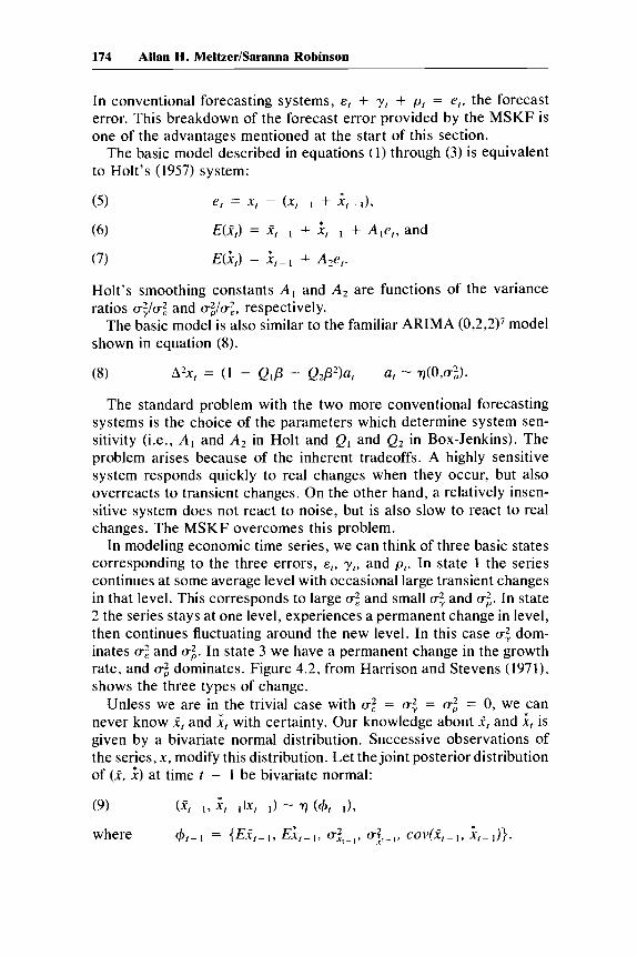
In conventional forecasting systems, E , + yr + p , = el, the forecast error. This breakdown of the forecast error provided by the MSKF is one of the advantages mentioned at the start of this section.

The basic model described in equations (1) through (3) is equivalent to Holt’s (1957) system:

( 5 ) e, = x, - (x, + i,-l),

(6) E(.f,) = + + Ale,, and

(7) E(&) = + A2e,.

Holt’s smoothing constants A , and A , are functions of the variance ratios u:/uz and uz/u$ respectively.

The basic model is also similar to the familiar ARIMA (0,2,2)7 model shown in equation (8).

(8) A2x, = ( 1 - Q1P - Q,P2)a, a, - q ( O , d ) .

The standard problem with the two more conventional forecasting systems is the choice of the parameters which determine system sensitivity (i.e., A , and A2 in Holt and Ql and Q2 in Box-Jenkins). The problem arises because of the inherent tradeoffs. A highly sensitive system responds quickly to real changes when they occur, but also overreacts to transient changes. On the other hand, a relatively insen- sitive system does not react to noise, but is also slow to react to real changes. The MSKF overcomes this problem.

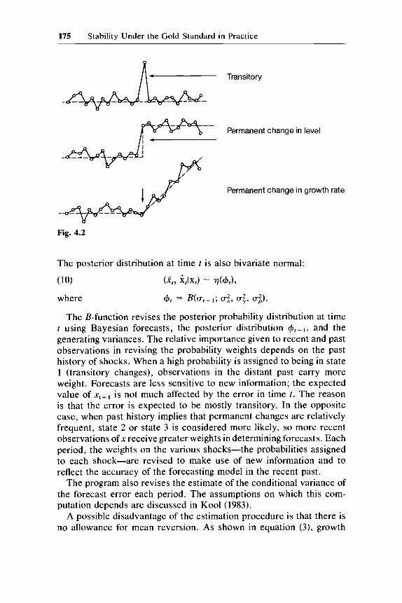
In modeling economic time series, we can think of three basic states corresponding to the three errors, E,, y,, and pl. In state 1 the series continues at some average level with occasional large transient changes in that level. This corresponds to large uz and small (.: and uz. In state 2 the series stays at one level, experiences a permanent change in level, then continues fluctuating around the new level. In this case u: dominates ~2 and uz. In state 3 we have a permanent change in the growth rate, and C T ~ dominates. Figure 4.2, from Harrison and Stevens (1971), shows the three types of change.

Unless we are in the trivial case with u; = a: = u;5 = 0, we can never know X, and if with certainty. Our knowledge about X, and i, is given by a bivariate normal distribution. Successive observations of the series, x, modify this distribution. Let the joint posterior distribution of (i, i ) at time t - 1 be bivariate normal:

(9) ( X t - 1 , i t - l l x f - 1 ) - q (4,-I).


F-- Permanent change in level

Permanent change in growth rate

Fig. 4.2

The posterior distribution at time t is also bivariate normal:

(10) (L b,) - r l ( + t ) ,

where +, = B(u,- 1; u;, u;, m;).

The B-function revises the posterior probability distribution at time t using Bayesian forecasts, the posterior distribution +,- I, and the generating variances. The relative importance given to recent and past observations in revising the probability weights depends on the past history of shocks. When a high probability is assigned to being in state 1 (transitory changes), observations in the distant past carry more weight. Forecasts are less sensitive to new information; the expected value of xt+ I is not much affected by the error in time t. The reason is that the error is expected to be mostly transitory. In the opposite case, when past history implies that permanent changes are relatively frequent, state 2 or state 3 is considered more likely, so more recent observations of x receive greater weights in determining forecasts. Each period, the weights on the various shocks-the probabilities assigned to each shock-are revised to make use of new information and to reflect the accuracy of the forecasting model in the recent past.

The program also revises the estimate of the conditional variance of the forecast error each period. The assumptions on which this computation depends are discussed in Kool (1983).

A possible disadvantage of the estimation procedure is that there is no allowance for mean reversion. As shown in equation ( 3 ) , growth


rates are pure random walks. However, if mean reversion is slow, errors from this source are largely offset by the revision of the weights each period. The random walk has the advantage of permitting the values currently expected for prices or output in the distant future to be computed from information available today. The forecast for k periods in the future, made at the beginning of time t , is

+ kx,- ,E(x, + k) = .f-

Another disadvantage of the MSKF procedure is that forecasts are based on a single time series. Information in related series is ignored. In practice, we have used vector autoregressions (VARs) to relate forecast errors for prices and output to lagged values. In previous work (Meltzer 1985) the VARs have added only a relatively small amount of additional information. This suggests that the MSKF procedure is relatively efficient.

In practice the MSKF combines six filter models to analyze the data. The six models decompose the data into two groups, with E, , Y,, and pt errors in each group. The two groups separate normal errors and outliers, the latter consisting of 5 percent of the errors. Separating errors into normal and outlier values permits the program to give less weight to large, one-time changes.

Since the MSKF model is equivalent to an ARIMA model with adjustable coefficients, forecast errors are typically smaller for MSKF than for the ARIMA model. An additional advantage is that each forecast depends only on data for periods prior to the time the forecast is made. In practice, of course, the forecasting technique was not available for most of the period. We treat the forecasts and errors as an approximation to the information available to a relatively accurate fore- caster at the time.

To evaluate the forecast accuracy of the MSKF, forecasts using several ARIMA models and a random walk* were generated for German prices and real output. The time periods are 1875-1913, 1950-72, and 1973-85, as in previous tables. Forecast errors are measured using both mean absolute percentage error (MAE) and root mean square error (RMSE). None of the alternative ARIMA models had MAE or RMSE values as low as the values for the random walk. Further, table 4.5 shows that, with minor exceptions, the MSKF performs as well or better than the random walk model under all monetary regimes and for both variables.

Comparison of the MSKF forecasts of prices and output to the means and standard deviations of actual price level and output series provides some additional information about the properties of the forecasts. These


Table 4.5 Comparison of Forecast Accuracy for Germany

Real Output Prices

Model GS BW FR GS BW FR

Errors measured using MAE MSKF 0.1 1 0.49 0.16 0.12 0.76 0.96 Random walk 0.40 0.48 0.16 0.73 0.83 0.94

Errors measured using RMSE MSKF 0.01 0.07 0.03 0.01 0.03 0.04 Random walk 0.05 0.07 0.04 0.04 0.04 0.03

Nofes: x - F1

x, MAE, = -- x 100.

RMSE, = V(X, - F? GS = gold standard; BW = Bretton Woods; FR = fluctuating rates.

F~ = forecast of&

are shown in table 4.6. The distributions of the MSKF forecasts very closely approximate the distributions of the actual series being forecast. In virtually all cases the means and standard deviations of the forecast values are equal to or within a few one-hundredths of the actual values.

Data for the period before World War I and after World War I1 are treated separately in our analysis. Wartime and interwar data are omitted. The reasons are that data are not available for all countries during wartime, and interwar data for German prices are affected by the hy- perinflation. This has a cost, however. The MSKF program uses some arbitrary values for the initial prior probabilities. Initial forecast values depend on these weights. In practice, this problem is reduced for several countries during the classical period by starting the analysis when the data series begin, but using only values for the classical period. Both sets of dates are shown in table 4.2 above.

We treat the annual data for 1950 to 1985 as one data set. An alternative procedure would analyze the two postwar regimes separately. It would remove the influence of the Bretton Woods period from the forecasts made during the early years of the fluctuating rate period. The shift in regime would be analyzed as a break in forecast patterns instead of a gradual transition with uncertainty about whether countries would return to a fixed rate regime. The tradeoff is that forecasts would depend considerably more on the arbitrary conditions assumed at the start of the new regime. This would have considerable impact in the fluctuating rate period which has only thirteen annual observations. The analysis, as performed, carries the probability weights from the Bretton Woods period into the start of the fluctuating rate period. The

178 Allan H. Meltzer/Saranna Robinson

Table 4.6 Descriptive Statistics: Actual Values and MSKF Forecasts

Means Standard Deviations

GS BW FR GS BW FR

R e d Output Denmark 7.41 9.41 10.01 0.24 0.3 I 0.06

7.44 9.45 10.02 0.25 0.31 0.06 Germany 9.82 13.43 14. I 6 0.28 0.43 0.08

9.82 13.50 14. i n 0.29 0.41 0.08 Italy 4.29 11.91 12.66 0.18 0.38 0.08

4.30 1 1.89 12.65 0.18 0.39 0.08 Japan 8.67 11.02 12.33 0.17 0.63 0.16

8.67 11.10 12.38 0.19 0.66 0.16 Sweden 7.66 9.78 10.34 0.33 0.28 0.05

7.68 9.82 10.36 0.33 0.28 0.05 U.K. 8.07 9.01 9.45 0.23 0.20 0.05

8.09 9.04 9.46 0.24 0.20 0.05 U.S. 4.36 14.24 14.79 0.30 0.24 0.09

4.40 14.27 14.81 0.30 0.24 0.09

Prices Denmark 3.98 6.02 7.30 0.08 0.31 0.34

3.97 6.06 7.39 0.08 0.33 0.33 Germany 4.37 3.80 4.55 0.08 0.20 0.16

4.37 3.83 4.60 0.08 0.21 0.14 Italy 3.02 2.88 4.43 0.08 0.26 0.60

3.02 2.87 4.42 0.09 0.27 0.60

3.09 3.53 4.56 0.12 0.28 0.15 Sweden 4.47 6. I 4 7.29 0.08 0.22 0.37

4.48 6. I 8 7.38 0.10 0.27 0.37 U.K. 3.96 5.84 7.26 0.06 0.25 0.47

3.96 5.88 7.38 0.06 0.26 0.46

3.26 3.67 4.58 0.12 0.18 0.27

Notes: For each country, first line is actual value, second line is MSKF forecast. GS =

gold standard; BW = Bretton Woods; FR = fluctuating exchange rates.

Japan 3.12 3.48 4.52 0.13 0.29 0. i n

U.S . 3.25 3.65 4.51 0.10 0.16 0.28

weights are then revised as new information arrives. The procedure we adopted has greater intuitive appeal as a model of learning about the consequences of a change in regime than the use of arbitrarily chosen values for the underlying variances and prior probabilities.’

4.4 Forecast Errors in Different Regimes

No monetary system can insulate output and the price level totally from real shocks to the economy. Monetary regimes can affect the variability of output and prices, however, and the size or frequency of


unanticipated disturbances. A welfare-maximizing monetary rule would reduce variability to the minimum inherent in nature and institutional arrangements. Since we do not know the welfare-maximizing monetary rule, we compare the relative performance under three monetary regimes: the gold standard, Bretton Woods, and fluctuating exchange rates.

Two measures of variability are available: the mean absolute error (MAE) of one-period-ahead forecasts and the root mean square error (RMSE). Since there are occasional large shocks or forecast errors, we rely on the MAE estimates for our comparisons to avoid excessive weight on large errors. This section compares the forecast errors for output and prices, computed using the MSKF program, for seven countries under the three regimes.

The estimates of E , y , and p permit computation of three measures of variability. The first, a measure of the variability of the level of the variable, is the sum of d + 7 + p, where the bar indicates the MAE. This measure is more useful for prices than for output, since price stability increases welfare while stable output with rising population implies a decline in per capita output. The second measure, + p, omits the transitory error in the level of output; 7 shows the variability of transitory changes in the growth rate of output and p shows the variability of permanent changes in the growth rate. Their sum gives the variability of the measured growth rate of output and the measured rate of price change. Third, we show 0, the mean change in the permanent growth rate of output and the maintained rate of inflation. pis a measure of uncertainty about sustained future growth and inflation.

Table 4.7 shows the data for the levels and growth rates of output. Several features deserve comment.

First, variability of output is usually higher under the gold standard then in the postwar regimes. The only exceptions are the United King- dom and Italy under fluctuating rates.

Second, there is considerable similarity in the MAEs of different countries under the gold standard. Denmark, Germany, and Italy have about equal values, as does the United States when a few large values are omitted. This suggests that common shocks may have dominated under the gold standard. To test this proposition, we computed the correlation across countries for each output shock ( E , y , p ) separately. The number of statistically significant positive correlations is considerably higher under fluctuating rates and Bretton Woods than under the gold standard, so the hypothesis is rejected.'O

Third, the United Kingdom and Japan have very different experiences under the three regimes. The United Kingdom has the lowest variability of any country under the gold standard and the second highest under fluctuating exchange rates. Japan suffered the greatest


Table 4.7 Mean Absolute Error Forecasts of Output and Growth (in percentages)

Classical Period Bretton Woods Fluctuating Rates

Country (1) (2) (3) ( 1 ) (2) (3) (1) (2) (3)

Denmark Germany Italy Italy" Japanb JapanC Sweden U.K. U.S. U.S.d

~~ ~

3.1 2.7 1.6 2.6 2.2 1.2 2.5 2.2 1.2 3.0 2.2 0.6 2.6 2.3 1.3 2.2 2.0 1.3 3.1 2.3 0.9 1.9 1.5 0.8 5.0 4.7 2.8

3.0 2.8 1.7 14.1 12.3 8.0 2.6 2.1 1.2 1.6 1.4 0.9 11.4 10.1 6.6 3.8 3.2 1.3 1.9 1.6 0.9 2.0 1.9 1 . 1 2.1 1.5 0.6 1.9 1.5 0.8 2.6 2.3 1.3 4.3 3.3 1.5 1.7 1.4 0.7 3.1 2.8 1.7 3.2 2.4 1.1

Note: (1) = output; (2) = growth; (3) = sustained growth rate. aOmits two largest errors, 1983 and 1984. hBased on Okhana's estimates of national income. Classical period includes 1880-96 under bimetallism and 1897-1913 on gold.

dOmits three largest errors-1893, 1895, 190&in classical period. four largest errors--1882, 1883, 1885, 1899-in classical period.

variability under the gold standard and benefited from the lowest under fluctuating rates.

Fourth, the United States has the lowest variability under Bretton Woods, although the differences with Sweden, Italy, or the United Kingdom are not large. The relatively low variability for the United States under Bretton Woods and for the United Kingdom in the classical period suggests that countries at the center of the exchange rate system may benefit from lower output variability. This would occur if, on balance, other countries absorb output shocks received from the center. There is some evidence of this for the gold standard, but not for the Bretton Woods system. The correlations of shocks show seven (out of a possible twenty-one) negative values in the range - 0.4 to - 0.5 under the gold standard. Five of the seven involve the United Kingdom. Under Bretton Woods and fluctuating rates, all statistically significant correlations are positive.

Fifth, the results for the United States are qualitatively similar to those based on quarterly data in Meltzer (1984). Variability of output and growth is highest under the gold standard. In part, the greater variability reflects relatively large errors in years of recession--1893 and 190&but the severity of recessions may reflect the operation of the gold standard. One difference from the quarterly data is that the variability of our measure of sustained growth, p, is slightly lower under the gold standard than under fluctuating rates. This finding differs from


the one based on quarterly data and suggests slightly greater stability of the anticipated long-term path of output relative to the fluctuating rate period.

Sixth, uncertainty does not increase uniformly under fluctuating exchange rates. Japan shows later variability on all measures, and variability in Germany and Denmark either declines or remains the same. The principal increases in uncertainty are in the United States, the United Kingdom, and Italy.

An alternative explanation of the higher variability experienced in some countries under the gold standard is that sectoral shifts in production have worked to make output less variable in recent years. The relative decline in agriculture and rise in manufacturing and services is often suggested as a principal reason for the change. This explanation fails to account for the experience of the United Kingdom, where variability is lower under the gold standard than under fluctuating rates, or of Germany, where the differences under the three standards are relatively small. Nevertheless, we tried to estimate the importance of change in output mix. To separate the effects of agriculture and manufacturing, we computed the variability of measures of industrial production under the gold standard for Germany and the United States. The MAEs for U.S. industrial production 1889-1913, comparable to columns ( 1 ) to (3) of table 4.7, are, respectively, 8.50, 6.54, and 2.70. For Germany, the computations are for 1875-1913, the same period used in table 4.7. The German values are 2.80, 2.24, and 1.00. The calculations for Germany do not differ importantly from the calculations for total output in table 4.7. For the United States all values are higher. Both calculations suffer from the fact that shocks to agriculture affect the demand for manufactures, the output of manufacturing in- dustries, and the series on industrial production. Neither the data for Germany nor for the United States show evidence, however, that the use of total output or GDP biases our result against the gold standard.

Finally, to pursue the issue of the relative variability of agricultural and industrial output, we computed the same measures of variability for a major crop in the United States and Germany under the gold standard. We chose corn production for the United States and rye production for Germany. The numbers reported are the same calculations as columns (1) to (3) in table 4.7. The values for U.S. corn are 15.42, 10.24, and 3.26, respectively, and for German rye, 9.44, 7.15, and 3.40. Under relative variability, the ratios of U.S. corn to U.S. industrial production are 1.8, 1.6, and 1.2; the ratios of German rye to German industrial production are 3.4, 3.2, and 3.4.

These data suggest that variability in the production of agricultural products was larger than the variability of industrial production under the gold standard. For Germany, where variability of industrial


production is lower than in the United States, relative variability for agricultural products is higher. Unlike the more ambiguous results for industrial production, the data on relative variability provide some evidence that the decline in the relative size of the agricultural sector may have contributed to the decline in variability over time. For Ger- many, the relative variability is large enough to reverse our previous conclusion. For the United States, this is not the case. Adjustment using the relative variability measure narrows the difference between the gold standard and the Bretton Woods, but does not change the ranking.

A problem with these results is that comparison of a single series on agricultural production to an index of industrial production may bias the result. This would occur if total agricultural production is less variable than any single crop. We have not pursued this issue or extended the calculation of relative variability to other periods.

While no single regime has the lowest variability of output growth in all countries, fluctuating exchange rates have the highest variability of output growth only in the United Kingdom and Italy. The data suggest that countries that follow medium-term predictable policies, like Japan, have been able to lower variability and uncertainty under fluctuating rates, while countries that follow less predictable policies- notably the U.S., the U.K., and Italy-have not. In the latter countries, policy actions shift more frequently from stimulus to restraint, increasing variability and uncertainty.

The U.K., the U.S. , and Italy shifted in the late 1970s or early 1980s from inflationary to disinflationary policies. The policy change was sharp and sudden, and the U.S., U.K., and Italy suffered a relatively severe recession followed by a relatively brisk recovery. In contrast, Japan experienced a comparable (or higher) rate of inflation in 1974 and 1975 as it, like Germany, maintained more gradual and persistent policies.

Italy, like Denmark, has a fixed but adjustable exchange rate with respect to countries in the European Monetary System and fluctuating rates against the pound, the dollar, and the yen. Variability of output and growth in Italy under fluctuating rates differs considerably from the experience of Denmark, however.

The contrasting experiences under the fluctuating rate regime suggest that differences in policy action and in the perceived degree of commitment to a stable policy are an important source of the difference in outcome. Fluctuating exchange rates do not enhance or prevent variability. They provide an opportunity to increase stability. Some countries have benefited from the opportunity, but others have not.

The results for prices and inflation show a similar, mixed pattern. Again, no regime dominates in all countries. Data for variability of prices and inflation are shown in table 4.8.


Table 4.8 Mean Absolute Error for Prices and Inflation (in percentages) ~~ ~~ ~ ~


Country (1) (2) ( 3 ) (1) (2) (3) (1) (2) (3)

Denmark Germany Italy Italy" Japanb JapanC Sweden U.K. U.S.

1.9 1.8 1.2 2.4 1.9 1.2 1.8 1.7 1 . 1 3.2 3.0 1.9 2.0 1.7 0.9 0.9 0.8 0.6 2.8 2.5 1.2 1.9 1.5 0.9 2.9 2.7 2.1

2.5 2.3 1.8 3.9 3.3 1.6 2.2 1.7 0.9 2.7 2.4 1.3

1.9 1.5 0.8 1.9 1.8 1.1 3.0 2.9 2.2 2.7 2.2 1.1 1.8 1.7 1.0 1.8 1.6 1.0 2.0 1.6 0.9 4.6 4.3 2.1 2.2 1.8 0.9 2.3 2.3 1.2 1.9 1.8 1.0

Nofe: ( I ) = price level; (2) = rate of price change; (3) = maintained inflation. "Omits 1974. bIncludes 1879-97 under bimetallism, with 1898- 1913 on the gold standard. 'Omits one large outlier: 1965 under Bretton Woods, and 1975 under fluctuating rates.

One of the claimed advantages of the gold standard is the reduced variability of long-run anticipated inflation. The annual data, like the quarterly data for the United States in Meltzer (1984), give little support to this claim. For most countries the variability of maintained inflation (table 4.8, column 3) is as high or higher under the gold standard than under Bretton Woods or the fluctuating rate regime. There is no evidence that the gold standard fostered long-term price stability as that term is used here."

Generally, prices and rates of price change have smaller forecast errors in one of the postwar regimes. The United Kingdom is, again, the exception since price level forecast errors are lowest there under the gold standard. For the United States, forecast errors are lowest under fluctuating rates, not under the Bretton Woods system.

The three regimes differ in the sources of price variability. The average MAE for the seven countries in the classical period is higher (2.7) than under Bretton Woods (2.3) or fluctuating rates (2.4). Each type of error, E , y , and p, is largest on average in the classical period. Transitory errors in level are smallest under fluctuating rates; fluctuating rates appear to buffer transitory shocks. Permanent shocks to growth are relatively more important under fluctuating rates than under Bretton Woods, reflecting the experience of Italy and the United King- dom. That experience suggests, however, that under the fluctuating rate system countries were less successful in buffering shocks to the perceived permanent rate of inflation than transitory shocks to the price level. Wage indexation following the oil shocks most likely contributed to this result for Italy in the 1970s.


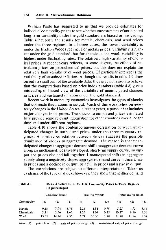
William Poole has suggested to us that we provide estimates for individual commodity prices to see whether our estimates of anticipated long-term variability under the gold standard are biased or misleading. Table 4.9 reports the results for metals, chemicals, and wool prices under the three regimes. In all three cases, the lowest variability is under the Bretton Woods regime. For metals prices, variability is highest under the gold standard, but for chemicals and wool, variability is highest under fluctuating rates. The relatively high variability of chemical prices in recent years reflects, to some degree, the effects of pe- troleum prices on petrochemical prices, but this does not explain the relatively high variability of wool prices. Of particular interest is the variability of sustained inflation. Although the results in table 4.9 draw on only a small part of the available data, they give no reason to believe that the computations based on price index numbers (table 4.8) give a misleading or biased view of the variability of unanticipated changes in prices and sustained inflation under the gold standard.

Recent work in monetary economics investigates the types of shocks that dominate fluctuations in output. Much of this work relies on quarterly changes in the United States in recent years, a period that includes major changes in oil prices. The shocks to output and prices estimated here provide some relevant information for other countries over a longer time and under different regimes.

Table 4.10 shows the contemporaneous correlation between unanticipated changes in output and prices under the three monetary regimes. A positive correlation between shocks suggests the possible dominance of shocks to aggregate demand. The reason is that unanticipated changes in aggregate demand shift the aggregate demand curve along an unchanged, positively sloped, short-run supply curve, so output and prices rise and fall together. Unanticipated shifts in aggregate supply along a negatively sloped aggregate demand curve induce a rise in prices and a decline in output, or a fall in prices and a rise in output.

The correlations are subject to different interpretations. Taken as evidence of the type of shock, however, they show that neither demand

Table 4.9 Mean Absolute Error for U.S. Commodity Prices in Three Regimes (in percentages)


Commodity ( I ) (2) (3) (1 ) (2) (3) (1 ) (2) (3)

Metals 9.38 7.74 3.73 2.24 1.81 0.98 5.25 1.73 3.16 Chemicals 3.11 2.66 1.65 1.26 1.09 0.55 10.57 8.46 5.50 Wool 15.63 14.44 8.53 13.71 10.30 3.78 21.78 11.84 6.38

Note: ( I ) = price level; (2) = rate of price change; (3) = maintained rate of price change.


Table 4.10 Correlations: Price Level and Output Forecast Errors

Country Classical Period Bretton Woods Floating Rates

Denmark 0.28 Germany 0.02 Italy -0.00 Japan -0.13 Sweden 0.12 U . K . -0.01 U.S. 0.20

- 0.88 -0.34 - 0.39 -0.18 -0.86 -0.85

0.15

-0.74 -0.51 -0.21 -0.74

0.04 -0.29 -0.66

or supply shocks dominate the contemporaneous correlations in all countries or under all regimes. The classical period shows no fixed pattern. The correlations are relatively small in all countries and are consistent with a mixture of supply and demand shocks. Such a pattern would arise from a mixture of productivity shocks in various countries and gold movements in response to changes in relative productivity and relative demand. Under Bretton Woods, the correlations are negative except in the United States, where the pattern is similar to that found for the classical period. The pattern under fluctuating rates is similar to that under Bretton Woods, with differences for individual countries, but the same mix of relatively high negative correlations in three or four countries and less clear-cut results in the remainder.

If we accept the evidence from the correlations, searching for the dominant type of shock is not likely to prove fruitful. This is not sur- prising. There is little reason to believe that shocks to aggregate demand or to aggregate supply dominate fluctuations of output and prices. Eco- nomic theory gives no reason for presuming that one or another type of shock dominates under all regimes.

A system of fluctuating rates permits countries to reduce shocks to aggregate demand from abroad. If under Betton Woods there were a mix of aggregate demand shocks from abroad and domestic or international shocks to supply, the shift to fluctuating rates would heighten the relative importance of supply shocks by eliminating (or reducing) the influence of aggregate demand shocks. The relatively strong oil shocks and the change in regime could then produce the observed change in the correlations for countries like Japan and the United States following the change in regime.

4.5 interaction Between Shocks

Prices and output are part of an interactive system in which shocks to one variable affect forecasts for that variable and others in the economic system. Also, shocks to one variable induce shocks to other


variables or to the same variable at a later date. The MSKF estimates ignore these interactions. In this section we discuss some efforts to go beyond the univariate system to explore interaction across countries and between shocks within a country.

To study the interactions, we use VARs to relate the shocks estimated using the MSKF. The VARs form a system of linear regressions of equal lag length relating, for example, the current price shock (or output shock) to lagged values of price and output shocks in the same country or in a foreign country.12

The VARs relating shocks to output and prices in the same country yield results not unlike the contemporaneous correlations. There is no dominant pattern. Some interactions between price and output shocks are negative, some are positive, but most are not significant by the usual standards.

We investigated the effect of introducing the interrelation between prices and output in the home country and in the country with the dominant currency-the U.K. in the classical period and the U.S. under the Bretton Woods system. Again, no consistent patterns were found, perhaps because the number of degrees of freedom becomes relatively small, particularly in the postwar regimes. To investigate this possi- bility, we computed the matrix of simple correlations between price shocks across countries for each type of shock and, separately, the simple correlation between output shocks. There are seven countries, so there are twenty-one correlation coefficients for each type of shock. The number of degrees of freedom differ in the different regimes, with the largest number for the gold standard and the smallest number for fluctuating rates.

Table 4.11 shows the number of correlations that are at least twice the computed standard error of the transformed correlation,

1 uz = ~ m’

where n is the number of observations and

I + r z = Y21n-

I - r

for correlation r. For prices, the number of correlations shown is largest under Bretton Woods and smallest under the gold standard. For output, the number of correlations in the table is highest under fluctuating rates. The latter may reflect the common oil shocks in the 1970s. Whatever the reason, it is clear that fluctuating rates did not prevent unanticipated shocks from affecting prices and output in several countries. Moreover, the effects on prices and output are found for permanent and transitory shocks.


Table 4.11 Correlations by Type of Shock and by Regime

Gold Standard Bretton Woods Fluctuating Rates

& Y P & Y P & Y P

Output Positive 1 2 1 6 6 6 7 9 9 Negative 3 2 2 0 0 0 0 0 0

Prices Positive 2 3 3 10 8 11 7 9 7 Negative 1 1 0 0 0 0 0 0 0

A notable difference between the gold standard and other standards is the finding of correlated negative shocks to output and prices. For the gold standard this is consistent with, and supportive of, the conclusion reached by Easton (1984) using deviations from trend of output. One plausible explanation is that under the gold standard, gold flows worked to expand output in one country and contract it in another, as the price-specie mechanism implies. This mechanism may have been strong enough to overcome the effects of common shocks arising from gold discoveries, technical changes in gold production, and changes in the demand for gold. Closer examination shows that both of the negative correlations for permanent output shocks involve the United Kingdom.I3 As noted earlier, this suggests that the United Kingdom may have succeeded in lowering output variability under the gold standard by allowing the London market to serve as an international financial market.

There are no similar findings for the United States under Bretton Woods. In fact, there are no correlations involving U.S. output in table 4.11 for the Bretton Woods period. For the price level and inflation correlations the situation is very different: five of the eleven correlations for p include the United States. Only Italy shows a relatively small correlation with the United States. It appears that the MSKF finds the expected interrelation between shocks to the maintained U.S. inflation rate and shocks to maintained inflation in other countries under fixed exchange rates. In contrast, only two of the eight correlations between permanent shocks to the price level under Bretton Woods involve the United States. It appears that one-time price level changes, estimated by y , did not diffuse internationally to the same degree as did persistent inflation under Bretton Woods, estimated by p .

Many of the papers in Bordo and Schwartz (1984) report mainly null results for interactions under the gold standard, similar to the results we obtained from VARs using annual observations. These findings are puzzling. The relation of prices in different countries under fixed


exchange rates has been reported for centuries. The problem may be the quality of the data, as some authors suggested, or the use of annual rather than quarterly data, or the relatively small number of degrees of freedom available.

To investigate the effect of using quarterly data, thereby increasing the number of degrees of freedom, we used available quarterly data for the United States and the United Kingdom under the gold standard. Gordon (1982) developed quarterly values of output and prices for the U.S.; Friedman and Schwartz (1963) provide quarterly data for the U.S. monetary base; and Capie and Webber (1985) constructed quarterly data for the U.K. monetary base. To study interaction under the gold standard, we estimated VARs relating shocks to the monetary base in the U.S. (BUS), the monetary base in the U.K. (BUK), U.S. real GNP and price deflator (RUS and PUS), for the period mid-1891 to mid-1914. Shocks were computed using the MSKF program separately on each of the series. The results of the VARs are shown in table 4.12 for four lags.

The quarterly data suggest statistically significant interactions between shocks to nominal and real values in the United States and the

Table 4.12 Vector Autoregressions for the U.S. and U.K. (4 lags, 18912 to 19142)

Dependent S u m of Variable Variable Lag Coefficients Significant Level RZ D W

B U S

R U S

P U S

B U K

B U S - 1.77 R U S 0.02 P U S 0.51 B U K - 0.23 B U S 0.67

P U S 0.77 B U K - 0.05 B U S -0.41 R U S 0.11 P U S -0.53 B U K 0.33 B U S 0.66 R U S 0.00 P U S -0.46 B U K - 0.43

R U S - 0.60

* 0.34 2.0

0.98 0.02 0.03 0.61 0.22 2.1 0.01 0.02 0.25 0.52 0.12 2.0 0.42 0.11 0.72 0.35 0.25 2.0 0.2 I 0.01 0.05

Norr: B U S = total shock t o U.S. monetary base: R U S = total shock to U.S. real GNP; P U S = total shock t o deflator: B U K : total shock to U . K . monetary base. Quarterly U.S. da t a from R U S and P U S a re from Gordon (1982): U.S. base from Friedman and Schwar t z (1963); U.K. base from Capie and Webber (1985). D W = Durbin-Watson statistic. *Less than 0.005.


United Kingdom. A main channel of interaction relates current and lagged values of shocks to the monetary bases in the United States and the United Kingdom with current and lagged values of shocks to prices and output.

Lagged shocks to the U.S. price level have a positive effect on the (unanticipated) U.S. base and a negative effect on the U.K. base of approximately the same magnitude after four quarters. An unanticipated increase in U.S. prices induces a transfer of base money (gold) from the U.K. to the U.S.; an unanticipated decline in U.S. prices induces an (unanticipated) outflow of gold. The lagged effect of the lower U.K. base reinforces the effect of higher prices on the U.S. base.

Past unanticipated prices have a positive effect on U.S. output; price and output shocks are positively related in the output equation, a pattern suggestive of demand shocks. Allowing for the lagged effects suggests a much stronger and more reliable relation between shocks to prices and output than is shown by the contemporaneous correlations. A 1 percent (unanticipated) increase in the price level raises output by 0.77 percent within four quarters.

The relatively strong and significant interaction between unanticipated prices and money poses two problems. First, the response of unanticipated money to unanticipated prices is opposite to the textbook description of the gold standard, where higher U.S. prices induce a flow of gold (base money) from the United States to the United King- dom or other countries. We investigated whether the four-quarter response reversed at longer lags. For values up to twelve lags, the effect of PUS on BUK changes to a positive (and statistically significant) sum, but the numerical value is small. Second, the estimates suggest that a change in unanticipated prices moves the system away from a purchasing power parity equilibrium, at least for a time.

Further, th.: large ( - 1.77) and statistically significant influence of lagged BUS on current BUS, and the smaller effect (-0.43) of lagged BUK on BUK suggests that stabilizing interaction under the gold standard may have depended much more on internal dynamics and capital movements and interest rates than on the price and output changes emphasized by price-specie-flow theories. The estimated responses of BUS and BUK to RUS are small and nonsignificant (0.02 and 0.00, respectively) and, as noted, the responses to PUS reinforce rather than stabilize BUS and BUK for periods up to three years.

On the financial side, we find that an unanticipated shift in gold or capital from the U.K. to the U.S. raises BUS and lowers BUK. Pre- sumably, interest rates rise in the U.K. and fall in the U.S. , but the lagged effects of BUS work to reverse the unanticipated increase in the U.S. monetary base and to offset the lagged effects of BUK on BUS. The lagged effects of BUK on current BUK reinforce the stabilizing properties of lagged BUS on current BUS.


The stabilizing effects of lagged own values of the unanticipated impulses may have been reinforced by the effects of price, output, and money anticipations. We have not investigated these channels. Further, our results come from a study of incomplete bilateral adjustment. We do not have quarterly data on prices and output in the United Kingdom, and we neglect changes in third countries that were part of the trade and payments system. For these reasons, our findings are, at most, suggestive of the way the gold standard may have worked in practice.

4.6 Conclusion

As Schwartz (1984, 1 1 ) notes, there are several hypotheses but little empirical evidence about the transmission of changes under the gold standard. Our study of unanticipated money, prices, and output begins to fill part of the gap and suggests that, at least for the United States and the United Kingdom, base movements played a dominant role in the international transmission of impulses. Price shocks as measured here had no role in achieving stability; the lagged effects of unanticipated price impulses appear to have reinforced expansive or contractive influences on output and money.

There are many explanations of the difference between the operation of the gold standard in the classical period before World War I and its operation during the interwar period. Our findings suggest that increased management of capital flows under the gold exchange standard may explain part of the difference. The data for the United States and United Kingdom suggest that capital movements, operating as unanticipated changes in the monetary base, were a main force stabilizing the system following price changes. Price and output impulses either had weak short-term stabilizing properties or worked to reinforce prior impulses. Price movements helped to stabilize the U.S.-U.K. system only, if at all, after a period of years. To the extent that central bank management reduced interwar capital movements, it reduced the stabilizing effects of lagged unanticipated values of the U.S. and U.K. monetary bases, thereby giving greater weights to the effects of past (unanticipated) price impulses. I4

A main aim of this study has been to compare the welfare properties of alternative monetary arrangements. The three monetary regimes we considered were the classical regime, when leading countries were on the international gold standard; the Bretton Woods regime; and the current fluctuating exchange rate regime. We used four criteria: rate of output growth, rate of inflation, and the stability of prices and of output growth. To compute variability of prices, output, inflation, and real growth, we relied on estimates from a multistate Kalman filter. The filter computes values for unanticipated levels and rates of change


of prices and output for each year, and allocates the unanticipated changes to three types of shock: permanent changes in the growth rate, permanent changes in level, and transitory changes in level.

We analyzed data for seven countries that differed in size, in the relative importance of trade, and in institutions. The countries were Denmark, Germany, Italy, Japan, Sweden, the United Kingdom, and the United States. Some countries established a link to gold very early in the nineteenth century. Some, like Italy, remained on the gold standard for only a brief period. We started the classical period about 1870, when several countries committed to maintain a fixed gold value of their currency. The classical period ends with the start of World War I, when most of the countries in our sample left the gold standard.

No single system dominated on all the welfare criteria. We do not attempt to weight the criteria to arrive at an overall judgment. Instead, we consider each criterion in turn.

The rate of inflation was lowest, on average, under the gold standard. The rate of growth was highest in most countries under the Bretton Woods system. The variability of prices and of output growth was highest for most countries under the gold standard. The main exception was the U.K.

There are well-known problems in making intertemporal comparisons, so the evidence of increased variability under the gold standard should be treated cautiously. One explanation, unrelated to the monetary standard, was the greater variability of agriculture and its greater relative importance in earlier periods. Some attempts to calculate the relative variability of industrial and agricultural production gave limited support to this proposition. For prices, the limited evidence for the United States did not support the hypothesis, but the limited evidence from individual commodity prices was difficult to interpret.

Some countries experienced greater stability under Bretton Woods, some under fluctuating exchange rates. We have found no evidence that the move to fluctuating exchange rates generally increased variability of output, prices, growth, or inflation. On the contrary, some countries achieved greater stability under fluctuating rates than under the alternative regimes. We conjecture that this result reflects the operation of credible, medium-term policies working either directly, or by stabilizing expectations, on the demand for money or velocity.

Using quarterly data for the United States from 1890 to 1980, Meltzer (1984) found that short- and long-term variability of prices and output was higher under the gold standard than in the postwar years. The annual data for the seven countries broadly support the same conclusion. In Meltzer, evidence of the much discussed long-term stability of prices under the gold standard comes mainly from ex post data showing that eventually the price level reverted to the value reached a half

192 Allan H. MeltzedSarama Robinson

century or a century earlier. In contrast, our conclusion is based on a measure of long-term price anticipations. The latter seems to us a more relevant measure of stability or uncertainty.

A byproduct of our work was some evidence on the type of shocks affecting the economies of the seven countries. We have found that experience differed under different regimes and between countries. No dominant pattern emerged. The search for a uniform cause of fluctuations would appear to be a misplaced effort.

Our results were subject to several limitations. The statistical model we use to compute impulses or shocks does not allow for mean reversion, an important part of the case for the gold standard. The gold standard provided a rule under which many felt confident that government policies would remain limited in scope. When governments adopted policies leading to temporary departures from gold or to devaluation, gold often provided an available means of protection for individuals. Although our statistical procedure is adaptive, it does not fully reflect these welfare-enhancing attributes of the classical gold standard.

There are other limitations. The forecasts and measures of shocks were based on data for periods prior to the period of the forecast, but the data on which we rely were not available at the time. And, as is well known, data for the nineteenth century are not entirely reliable. Further, we have not attempted to hold constant other relevant factors affecting output and prices, including weather, changes in output mix, and changes in nonmonetary policies.

Despite these and other limitations, there is sufficient uniformity in our results to support two propositions. First, short- or long-term anticipations about prices and output were less stable under the gold standard than under the monetary arrangements of the past thirty-five years. Second, a fluctuating exchange rate regime does not impose greater uncertainty and instability. Some countries were able to reduce uncertainty about prices and output under the fluctuating exchange rate regime, both absolutely and relative to Bretton Woods and to the classical gold standard.

Appendix Data Sources

EUROPEAN COUNTRIES: Data on prices and output before World War I are from Mitchell (1976). Postwar data are from OECD, various issues. German industrial and rye production from 1875 to 1913 is from Mitchell (1976, 355-56, 241, 254).


JAPAN: Data for output from 1878 to 1913 are Okhana’s estimates of real income. Price data are for 1873-1913. Both series are from Bank of Japan (1966). Postwar data are from OECD, various issues.

UNITED STATES: Data for output and prices before World War I are Net National Product (Kendrick) and implicit GNP deflator (Kendrick) from U.S. Department of Commerce (1966). Industrial production is Frickey’s index, 1889-1913, the U.S. Department of Commerce series (1960, 13), and the Federal Reserve index of industrial production, 1950-85. Metals prices and chemical prices are from Warren and Pear- son to 1890 and the Bureau of Labor Statistics after 1890; see Com- merce (1960), series E7, E9, E20, and E22 extended to 1985 using Bureau of Labor Statistics data. Corn production from 1889 to 1913 is from Commerce (1960), series K266.

Notes

1. There were suspensions of the gold standard and, in some countries, devaluations against gold even in the classical gold standard period. See Ei- chengreen (1985,6) for a list of countries that devalued. Mussa (1986) compares variability of ex post real exchange rates under fixed and fluctuating exchange rates in the postwar era.

2. Expansion of trade under fixed exchange rates achieved by increasing variability of prices and output is not a clear welfare gain. Further, evidence on the relation between exchange rate regimes and the volume of trade is, at best, mixed.

3. The periods are given in table 4.2 below. All end in 1913. 4. For expositional purposes, we take the optimal rate of inflation to be zero. 5. Schwartz (1981) finds a negatively sloped gold supply curve for the postwar

period, so the mechanism has not worked the same way in all periods. 6. A more complete discussion is in Bomhoff (1983, chapter 4) and Kool

(1983). 7. Testing the data for each country using standard Box-Jenkins identification

techniques indicates that second differencing is required to achieve stationarity in almost all cases.

8. We use last period’s actual value as this period’s forecast. 9. The computations of E, y and p begin in 1952, so there are twenty-one

years of fixed rates and thirteen years of fluctuating rates. 10. The correlations are discussed more fully below. 1 1 . The random walk in the anticipated growth rate does not incorporate

mean reversion, as noted earlier. 12. While the VARs help to compensate for our neglect of interactions be-

tween variables, they introduce a different problem. The estimates are no longer “true” forecasts. Estimates for a particular period now depend on events that occur later in the sample period.

13. The two countries are Denmark and Italy. The negatively correlated price shocks are for the United Kingdom and Germany.

194 Allan H. Meltzerharanna Robinson

14. Rich (1984) found that price movements worked to stabilize the U.S.- Canada bilateral system only over relatively long periods.

References

Bank of Japan, Statistics Department. 1966. Hundred year statistics of the

Bomhoff, E. 1983. Monetary uncertainty. Amsterdam: North-Holland. Bordo, M. 1981. The classical gold standard: Some lessons for today. Federal

Reserve Bank of St. Louis Review 63 (May): 2-17. -. 1986. Explorations in monetary history: A survey of the literature.

Explorations in Economic History 23: 339-415. Bordo, M., and A. J. Schwartz. 1984. A retrospective on the classical gold

standard, 1821-1931. Chicago: University of Chicago Press. Capie, F., and A. Webber. 1985. A monetary history of the United Kingdom,

1870-1982. Vol. I , Data, sources, methods. London: Allen and Unwin. Commission on the Role of Gold in the Domestic and International Monetary

Systems. 1982. Report to the Congress. Vol. 1. Washington, D.C. Cooper, R. 1982. The gold standard: Historical facts and future prospects.

Brookings Papers on Economic Activity I : 1-45. Easton. S. T. 1984. Real output and the gold standard years, 1830-1913. In

Bordo and Schwartz (1984, 513-38). Eichengreen, B. 1985. Editor’s introduction. In The gold standard in theory

and history, ed. B. Eichengreen, 1-35. New York: Methuen. Friedman, M., and A. J. Schwartz. 1963. A monetary history of the United

States, 1867-1960. Princeton: Princeton University Press. Gordon, R. J. 1982. Price inertia and policy ineffectiveness in the United States,

1890- 1980. Journul of Political Economy 90: 1087- 1 1 17. Harrison, P. J., and C. F. Stevens. 1971. A Bayesian approach to short-term

forecasting. Operational Research Quarterly 22:341-62. Holt, C. C. 1957. Forecasting seasonals and trends by exponentially weighting

moving averages. Pittsburgh: Carnegie Institute of Technology. Klein, B. 1976. The social costs of the recent inflation: The mirage of steady

“anticipated” inflation. Carnegie Rochester Conference Series on Public Policy 3:185-212.

Japanese economy. Tokyo: Bank of Japan.

Kool, C. J. 1983. Appendix 1. In Bomhoff (1983, 227-46). Meltzer, A. H. 1984. Some evidence on the comparative uncertainty experi-

enced under different monetary regimes. In Alternative monetary regimes, eds. C. D. Campbell and W. R. Dougan, 122-53. Baltimore: Johns Hopkins University Press.

-. 1985. Variability of prices, output and money under fixed and fluctuating exchange rates: An empirical study of monetary regimes in Japan and the United States. Bank of Japan Monetary and Economic Studies 3

-. 1988. On monetary stability and monetary reform. In Toward a world of economic stability, eds. Y . Suzuki and M. Okabe. Tokyo: University of Tokyo Press.

Mitchell, B. 1976. European historical statistics, 1750-1970. New York: Co- lumbia University Press.

(3): 1-46.


Mussa, M. 1986. Nominal exchange rates and the behavior of real exchange rates: Evidence and implications. Carnegie Rochester Conference Series on Public Policy 25:117-214.

Rich, G. 1984. Canada without a central bank: Operation of the price-specie- flow mechanism, In Bordo and Schwartz (1984, 547-75).

Rockoff, H. 1984. Some evidence on the real price of gold, its costs of production, and commodity prices. In Bordo and Schwartz (1984, 613-44).

Schwartz, A. J. 1981. Gold output. Memo to the members of the Gold Com- mission, September.

-. 1984 Introduction. In Bordo and Schwartz (1984, 1-20). -. 1986 Alternative monetary regimes: The gold standard. In Alternative

monetary regimes, eds. C. D. Campbell and W. R. Dougan, 44-72. Balti- more: Johns Hopkins University Press.

U.S. Department of Commerce, Bureau of the Census. 1960. Historical statistics of the United States, Colonial times to 1957. Washington, D.C.: GPO.

U.S. Department of Commerce, Bureau of the Census. 1966. Long-term economic growth, 1860-1965. Washington, D.C.: GPO.

Comment William Poole

I enjoyed reading the Meltzer-Robinson (hereafter, MR) paper,' and learned a lot from it. There are two aspects to this work. First, MR provide a compact summary of inflation and output data for seven countries and a commentary on the principal issues. Second, they provide a detailed analysis of their data using the multistate Kalman filter.

My concerns about the Kalman filter in the context of this paper involve the small number of observations and the quality of the data. It appears that MR estimate a substantial number of parameters from relatively few observations. The maximum number of observations during the classical period is 44 for the United Kingdom; the Bretton Woods and floating rate periods taken together contain 36 observations. The results must depend heavily on the a priori specification. For the Bretton Woods and floating rate periods, the Kalman filter forecasts and forecast errors are calculated from 23 and 13 observations, respectively. Given that the floating rate period has only 13 observations, I would be a little more cautious in drawing general conclusions about floating rates than are MR. As for the quality of the data, MR do develop a strong case by examining a number of different countries and several different series for some countries.

Tables 4.7 and 4.8 provide the basic findings of the paper. Although the results are not uniform across countries and across periods, in

William Poole is a professor of economics and the director of the Center for the Study of Financial Markets and Institutions at Brown University, Providence, Rhode Island.


general the classical period had somewhat higher variability of output forecast errors from the Kalman filter than the Bretton Woods and flexible exchange rate periods. I read table 4.8 as essentially a draw in comparing price forecast errors during the classical period and the post- World War I1 periods. These tables do not provide support for arguing the superiority of the gold standard.

Table 4.6 shows that the Kalman filter forecasts have means and standard deviations that are close to those of the actual data, indicating that the Kalman filter forecasts and the actual data have similar statistical properties. I would have expected the standard deviations of the Kalman filter forecasts to be significantly lower than those of the actual data, on the grounds that efficient forecasts cannot pick up the random component in the levels of the data. The results in table 4.6 arise because the levels data are nonstationary, or approximately so; levels disturbances account for a small part of the standard deviations of these series. Note 7 reports that second differencing is required to achieve stationarity, and table 4.5 shows that for Germany the Kalman filter and random walk models are essentially the same for both the Bretton Woods and flexible rate periods. My guess is that repeating table 4.5 for the other countries would yield similar results.

In table 4.5 the Kalman filter forecasts are more accurate than random walk model forecasts only for the classical period. The reason, no doubt, is that the classical period has two distinctive subperiods divided by 1896, as table 4.1 shows. The Kalman filter adjusts its forecasts when going from one subperiod to the next, which the random walk model cannot do.

MR focus attention on errors from Kalman filter forecasts, and they argue that the errors are likely to be related to welfare costs, However, they note that stability of output levels does not enhance welfare. Table 4.7 should be read in conjunction with table 4.3. For most countries, growth was high and more stable during the Bretton Woods period than during either the classical or floating rate periods.

In many applications the purpose of using a filter is to obtain efficient forecasts. Efficient forecasts may be relatively little affected by errors in the data; one of the purposes of any filtering technique is to deal effectively with data errors. But in the MR application, the name of the game is to estimate the forecast errors themselves. Data errors are included in these estimates, and surely the nineteenth-century data have larger errors than the post-World War I1 data. Also, price indexes after World War I1 include many more goods which tends to make these series less variable than nineteenth-century series constructed from relatively few goods.

The fact that the mean absolute errors in tables 4.7 and 4.8 are of the same order of magnitude for the gold standard and floating rate

1W Stability Under the Gold Standard in Practice

periods suggests that the “true” errors-that is, the forecast errors’ net of data errors-may well have been smaller during the gold standard era. However, table 4.9 does not support this hypothesis for several U.S. commodity price series, which are presumably of reasonably consistent quality over time.

Data construction may also have something to do with the results in table 4.10 which reports correlations between price and output forecast errors. There is a striking difference between the correlations for the classical era and the post-World War I1 era. I think it is correct that data on GNP or GDP after World War I1 start with nominal magnitudes, which are than split into real and price parts. Thus, errors in the price data create equal and opposite errors in the quantity data and could explain, in part, the negative correlations in table 4.10 for the Bretton Woods and floating rate periods. Moreover, when the implicit deflator is used as the price variable, cyclical changes in the composition of constant dollar GNP tend to create a negative correlation between the deflator and constant dollar GNP. Were the data for the classical era constructed in about the same way, or might a difference in construction explain the arithmetically larger correlations for the classical period?

Negative serial correlation of price changes has been an important part of the case for the gold standard, but table 4.4 does not support the case. Before I accept the fine detail of these results, I need to know more about the data. We know that constructing annual data by av- eraging monthly data induces a spurious positive serial correlation of changes. There is also the issue of the extent to which nineteenth- century data were constructed using interpolations. Nevertheless, data construction is surely not responsible for the fact that the classical period consisted essentially of a long deflation followed by a long inflation. The case for negative serial dependence cannot be built on such evidence for there are only two observations: one deflation, followed by one inflation.

Let me now turn to table 4.12 and the discussion surrounding it. The interactions across countries is an interesting and important topic, but I am uneasy with the story MR try to extract from vector autoregressions. Note that MR apply the VARs to the shocks estimated from the Kalman filter. It is certainly possible that the Kalman filter forecasts, which represent the systematic part of the individual series, display relationships across countries that exactly fit the classic gold standard mechanisms.

The VARs may be telling us that the forecast errors computed from the Kalman filter are higher than they should be. MR note that the Kalman filter ignores interactions across variables. If table 4.12 is read as suggesting that there are indeed some interactions of modest statistical significance, then the calculated Kalman forecast errors discussed


earlier in the paper may not be a reliable guide to comparing variability across countries and exchange rate regimes. However, because the VARs do not identify highly significant interactions it is reasonable to conclude that the forecast errors defined by the univariate Kalman filter approximate the errors that economic agents would actually make in practice.

I question MR’s interpretation of table 4.12. For example, they are concerned about the positive effect of prices on the base as reported in the first VAR in table. But in the VAR context, the price disturbance cannot be interpreted ceteris paribus. The price disturbance initially raises BUS, but lagged BUS lowers BUS. Moreover, in the VAR for PUS, lagged BUS reduces PUS. Without simulating the system, it is impossible to see how all this will work out. MR suggest as much in their comment that capital flows and interest rates may have played an important role. It would have been possible to include interest rates in the VAR, but I would not hazard a guess as to the result or how to interpret the result once I saw it.

MR conclude that the short- and long-term variability of both output and prices was higher under the gold standard than during the postwar years. To support this conclusion it would be helpful if MR would report results in tables 4.7 and 4.8 for the Bretton Woods and fluctuating rates periods combined. To my taste there are too few observations under floating rates to have great confidence in statistical results for this period. As MR note when discussing the average rate of inflation under floating rates, it is misleading to attribute the economic ills of the 1970s to the floating rate system; these ills were, in part, left over from Bretton Woods.

My suspicion is that MR’s conclusion on variability is correct for output, but probably not for prices. Table 4.8, as it stands, is essentially a draw, but the inflation section of table 4.3 leaves the gold standard a clear winner. The two gold standard subperiods defined in table 4.3 each delivered average inflation rates closer to zero than did the Bretton Woods and floating rate periods. Economic welfare depends on the average inflation rate as well as on inflation forecast errors, perhaps because in practice economies do not fully adjust to ongoing inflation.

MR do not attempt to weight the price and output results to arrive at an overall welfare judgment. There is reason, however, to emphasize the price results. The argument is not that price stability is more important than output stability, but that we are comparing alternative monetary systems rather than alternative output systems, such as central planning versus the market. The monetary system is the primary determinant of price performance, but perhaps only a minor determinant of output performance. There is certainly a substantial amount of evidence that output growth and inflation are, at best, very weakly related.


There is another way to put this point. If the gold standard did not deliver price stability, then the argument is over. But it is reasonable to conclude that the gold standard did deliver price stability in greater measure than other approaches tried since 1914. The stability was not as great as the gold enthusiasts would have us believe, but for the reasons I have discussed, the stability was probably greater than MR have concluded.

I agree with MR that the case for mean reversion of the price level under the gold standard is not strong, at least in terms of a strict interpretation of that hypothesis. The first part of the classical period involved deflation and the second part involved inflation. If the claim is that the deflation caused an increase in gold production and the subsequent inflation, then these data by themselves contain too few observations to test the hypothesis. The mean reversion hypothesis should not be taken literally anyway. There is no reason whatsoever to believe that the equilibrium relative price of gold is a constant.

But the case for the gold standard does not rest on the fact that inflation from 1896 to 1913 cancelled out deflation from 1873 to 1896. Either of these periods taken separately exhibited satisfactory price performance by today’s standards. The average rate of inflation or deflation was relatively low. The year-to-year variability appears high by today’s standards, but that is at least partly illusory. Some of the greater variability of the inflation rate in the nineteenth century reflects the relatively narrow scope of available price indexes, while some of the apparent smoothness of postwar inflation reflects an ex post rather than an ex ante calculation of the average inflation rate. That is the point of MR’s Kalman filter analysis, and it shows up in the results reported in table 4.8.

I agree with MR’s skepticism that long-term price predictability pro- motes investment in durable capital. Most of us believe that a less predictable price level must surely lead to a less efficient allocation of resources, but the methods available to hedge price surprises seem extensive enough to keep the costs relatively low. Distributional effects, which seem to be fairly random across income classes, are greater and they are probably the source of much of the political dissatisfaction caused by unstable prices. Issues of equity and political stability are outside the scope of the MR paper, but given their broad overview of the subject, brief mention of these issues seems in order.

MR comment that the costs of maintaining long-term price predictability include those arising from returning to an established parity, as with Britain in 1821 and 1925. There are economic costs in these cases, but MR emphasize that there are benefits to wealthowners in the form of protection from confiscatory actions of government. I would add that there are also broad political benefits for any government that wants to maintain a reputation for reliability. A government cannot


break its economic commitments without raising questions about its reliability in other areas, such as its reliability as a treaty partner.

Finally, we should be careful to select appropriate criteria upon which to judge the gold standard. Early in the paper MR argue that, “[iln place of the long-term commitment to a fixed nominal exchange rate of domestic money for gold, countries could have made a commitment to a stable expected price level.” Given the state of knowledge of monetary economics in the nineteenth century, the gold standard was the logical arrangement to achieve a stable expected price level. Al- though the gold standard is, I believe, no longer a suitable monetary system, the fact that reputable economists and not just cranks believe that the gold standard is worthy of serious consideration even today is a tribute to the system.

Note

I . The Meltzer-Robinson paper was revised several times after the conference, as was my discussion. I regard my interchange with the authors as unusually fruitful, and wish to thank them for being so responsive to my comments and for their useful suggestions on my written discussion. However, the standard disclaimer applies: errors in my discussion are my responsibility (and errors in their paper are their responsibility).

General Discussion

MCCALLUM doubted the finding of long-run inflation unpredictability under the gold standard. In terms of an ARIMA formulation, this disbe- lief amounts to skepticism that inflation rates were not covariance stationary-that it was necessary to second difference the log of the price level. He presented evidence suggesting that second differencing was not necessary. He described the results of some ARIMA calculations, estimating (0,3,2) models and also very simple models-(O,l , I ) and (1,l ,O)-that use first differences of the log of the price level for five countries excluding Italy, which was not on the gold standard, and Japan, for which he did not have the data. In all these cases, very simple first-difference models outperformed the second-difference models in the sense that, basically, they are equivalent in terms of explanatory power. So there is no advantage to the more general specification. Thus, at the level of an ARIMA analysis, according to McCallum, it is just not the case that there seems to be any evidence


in favor of the second-difference formulation, which the Meltzer- Robinson setup represents. Furthermore, he conjectured that second differencing the data would be as inappropriate for Kalman filter models as he found it to be for the ARIMA models.

Finally, he pointed out that estimation of an ARIMA (0,2,2) model, as in equation (8) of the paper, revealed that for four out of five countries the sign of the second moving average coefficient was opposite to that predicted by the model.

MELTZER responded that, based on a comparison of ARIMA models on line to the multistate Kalman filter model on line, in most cases, the multistate Kalman filter had lower standard errors of forecast than the other models. [These results are reported in the published version of the paper.] He also pointed out that the calculations should not be interpreted as a statement about the gold standard but about the performance of the gold standard relative to other standards.

STEIN suggested looking at the variation of output around capacity output as a measure of the ability of different regimes to adjust to monetary shocks. He doubted the Meltzer-Robinson conclusion that price predictability was any better under floating rates than in previous periods, citing a paper by Robert Barro in the Journal of Business (1986) that showed interest rates to be poor predictors of inflation, particularly after 1971.

B. FRIEDMAN pointed out that the Kuznets-type of GNP estimates used in the study were based on the components of GNP that were likely to be the most variable. He suggested the use of Christina Ro- mer’s new industrial production and GNP estimates. He also wondered whether sectoral shifts in the composition of economic activity over time would be in the direction of dampening fluctuations-that the greater degree of variability during the gold standard period may be due, in part, to the higher share of agriculture relative to manufacturing and services in total production during that period. [The published version of the paper finds this not to be the case.]

WOOD wondered how evidence that long-term bond yields exhibited much greater stability under the gold standard than in the past thirty- five years could be reconciled with the conclusion of the paper that price unpredictability was higher under the gold standard than in the recent period, particularly bearing in mind the stability of the real rate of interest that Friedman and Schwartz reported in Monetary Trends.

MELTZER responded that looking at the actual movements of interest rates cannot tell you much about unanticipated variability.

KOCHIN made the point that an investor in 1910 would have been trying to predict the price level in 1919, not the conditional predicted price level assuming that the world gold standard would persist to 1919. In fact, in 1919 the world was off the gold standard.


For ten-year forecasts of the price level, the chance of going off the gold standard was always significant. All transitions off the gold standard are ignored in this study since data off the gold standard was excluded.

Moreover, comparing periods when the world was on the gold standard with those when it was not, biases the case in favor of the gold standard because it is a system which, when there is a big shock such as World War I, the world will abandon. The paper thus compares one data set where the shocks are excluded with another where the shocks are included.

MELTZER responded that the Kalman filter gives an on-line forecast, and to the extent that such factors entered into people’s heads, it should affect the permanent shock or the rho component. To the extent that it is there and is systematic, it is taken out as anticipated.

B. FRIEDMAN suggested that the authors include measures of the actual variability of monetary growth, inflation, and real output growth as a benchmark for comparison to the forecast errors. [The final draft of the paper incorporates this suggestion.]

WHITE suggested that, in order not to bias the historical comparison between the gold standard and fiat money regimes, one would also want to include fiat money episodes that have blown up, for example, the interwar period.

CHOUDHRI made the point that the difference between the standards may be due to measurement errors or real shocks. But these errors or shocks might be country specific, due, e.g., to Japan, so that an interesting test might be to compare the variance of errors across countries.

CARLINER suggested that the variability of prices and output over time might depend on common forces affecting all countries, such as improvements in the technology of financial systems or the shift out of agriculture.

LAIDLER doubted that, during the gold standard period, agents could satisfactorily predict prices and output in the way the paper assumes they were doing. The historical data used today were not available to them at the time. This, he argued, is an example of a problem that is always present when one uses historical data. We know much more about what is going on in historical time series than did the agents whose behavior generated them.

MELTZER responded that such a line of criticism pertains to all historical research. He pointed out that the data available to agents, at least for the 1920s, were not that different from what are available today.

stability under the gold standard in practice · 4 stability under the gold standard in practice...

Documents