Stability of Pull Production Control Methodsfor Systems with Significant Setups

Thomas I. Seidman∗ Lawrence E. Holloway†

IEEE-Trans. Auto. Control 47, pp. 1637–1647, (2002).

AbstractIn manufacturing, a pull production control method is a method

of authorizing production based on replenishing current and past con-sumption, as opposed to forecasts or orders for future consumption.In this paper, we consider special classes of pull systems for opera-tions that involve significant setup times. In particular, we presenta model for variations of the Signal Kanban method and the PatternProduction method, each of which is used in industry when conven-tional Kanban methods are inappropriate. This paper examines suchsystems under demands with unpredictable load content but an upperbound on the total load. It is shown that, under appropriate condi-tions, such systems are stable in the sense that cumulative productionat any time trails cumulative demand by no more than a constant.We determine buffer parameters under each protocol (including re-order points in the Signal Kanban case) such that the backorder queuewill clear to zero and remain empty thereafter. The results are thenextended to consider multiple machines fulfilling production autho-rizations in parallel.

Key Words: Production control, Signal Kanban, Pattern Production,lean manufacturing, round robin.

∗Department of Mathematics and Statistics, University of Maryland BaltimoreCounty, Baltimore, MD 21250, e-mail: 〈seidman@math.umbc.edu〉

†Center for Robotics and Manufacturing Systems University of Kentucky, Lexing-ton, Kentucky 40506-0108 e-mail: 〈holloway@engr.uky.edu〉 This work has been sup-ported in part by NSF Grant ECS-9807106, USARO Grant DAAH04-96-1-0399, and theUniversity of Kentucky Center for Robotics and Manufacturing Systems.

1

1 Introduction

Pull production control is an important tool used by companies operatingunder “just-in-time” manufacturing or “lean manufacturing” [9, 16, 15]. Inconcept, the pull production control method constrains the buildup of inven-tory by only authorizing production based on actual downstream consump-tion of product. Thus, in pull systems, authorizations for production comefrom downstream stations (hence, with demand arriving at the end of theline), in contrast to “push” production control systems, where orders arriveat the start of the line based on forecasts or orders for future consumption[9].

Most work in the literature on pull production control focuses on single-card Kanban1, two-card Kanban, and pull system variants such as CONWIP.A recent survey of Kanban methods is presented by Akturk and Erhun [1],and a comparison of these and other methods is given by Bonvik, Couch, andGershwin [2].In these classic implementations of Kanban, there are multipleproduction authorizations associated with a given product, and each one isassociated with a standard lot of product. Whenever such a lot begins to beconsumed, the authorization associated with it is released to the producingsystem, authorizing production to replenish it. Inventory is directly cappedby only having fixed numbers of such authorizations circulating in the system.

Such a system works well when the producing station is able to changeover between products relatively quickly and easily. In systems with sig-nificant costs or time associated with setups, the classic Kanban methodsare inappropriate. A balance must be reached between the need to limit thenumber of setups to avoid sacrificing capacity and the goals of small lot sizes,minimum inventories, and production smoothing which are emphasized in alean manufacturing operation. Instead, two different kinds of pull control arecommonly used. The first of these is the “Signal Kanban”. In contrast toclassical Kanban methods, a single production authorization (called a signalkanban) is associated with each product, and, in particular, with a specificlevel of inventory. When inventory falls below that level, the authorization isreleased to replenish the consumption. Signal Kanban production control isdiscussed by Monden [9]. In traditional inventory control theory, the SignalKanban method is often called a reorder point policy, or a two-bin system [8].

1As is common in the literature, we use the capitalized term Kanban to indicate theproduction control method, and the non-capitalized term kanban to indicate a productionauthorization within the method.

2

Such systems are commonly used in industry for operations with significantsetups or minimum batch sizes. In fact, our investigation of Signal Kanbansystems was motivated by the production control systems formerly in use atthe metal stamping line at Toyota Motor Manufacturing Kentucky (TMMK).

A second type of production control for use in systems with significantsetup costs is Pattern Production. In this control method, there is a fixedproduction sequence (pattern) and whenever the system receives such an au-thorization, it produces up to a fixed level to replenish past consumption.When the replenishment is complete, the machines are changed over to re-plenish the next product in the sequence. There is no specified minimumbatch size and no idle time for such a system. The time between repetitionsof the cycle is variable, in contrast to the cyclic productions considered inEconomic Lot Scheduling Problems [4].

A key point of the systems that we consider is that the inventory behaviorfor each product depends on the state of all other products which consumecapacity of the production system. In the case of Signal Kanban systems,the lead time of a production authorization depends on the number of otherdifferent products which are also waiting to be replenished, and in some caseson the volume of each product that must be replenished for each. Thus, thelead time depends indirectly on the past demand for all of the productsthat rely on a given machine or set of machines. In the case of the PatternProduction system, the period between replenishments of a product dependson the run-lengths of all other products run in the intervening period, andso again is dependent indirectly on past demand for all other products.

Our focus in this paper is on the stability of such pull production controlmethods for systems with significant setups. A production system is saidto be stable if all its buffers are bounded so cumulative production can trailcumulative demand by no more than a constant lag [10]. Certainly, tradi-tional capacity constraints are needed to have any possibility of stability.However, examples are known of layouts and systems with such simple con-trol policies as clearing [7] or first-come first-served [11] which satisfy thoseconstraints but are nevertheless unstable. Seidman and Humes [14] have ob-served examples of instability in the context of a production kanban systemwith orders based on consumption but serviced according to a clearing pol-icy. A principal distinction between that setting and our present concerns isthe treatment of multiple machines supplying each other. This is outside thescope of this paper, restricted to a single focus (whether comprised of onemachine or several), but is deferred to [13].

3

Our main result here is that, for appropriate selections of buffer param-eters, we show that Signal Kanban policies and Pattern Production policieswill be stable (the queue of backorders is bounded) and even strongly clearing(the backorder queue eventually becomes empty and remains there), subjectto a capacity constraint and a limit on the burstiness of total demand. Oneimportant implication of this result is that demand among different productscan be reallocated, as long as the burstiness bound on the total demand is notexceeded. We emphasize that the policies we consider determine productionsolely in response to demand, and no prior schedule or demand forecasts areassumed. Thus, the policies require no prior knowledge of the composition ofthe load or of the nature of the burstiness except that the limit is maintained.

In the next section, we describe our basic model of a production system.Section 3 shows stability of two common variations of Signal Kanban systems,fixed-fill and fixed-batch for a single machine operation. Section 4 presentsresults for pattern production control for a single machine. Section 5 consid-ers these protocols operating with a bank of machines servicing productionauthorizations in parallel.

2 System Overview

The structure of the systems we consider is shown in figure 1. There areN products (each associated with a buffern of size Bn). Demand (orders)arrive to the queue Q. If there are no backlogs, then the order immediatelyproceeds to the head of Q. The order at the head of Q is then filled withproduct from the corresponding buffern if it is nonempty. Otherwise, theorder remains as a backlog and also blocks subsequent orders until it can befilled.

Let Un(t) be the cumulative number of orders for productn arriving bytime t — including any ‘initial condition’. Thus, Un(0) = 0 means thatbuffern is initially full and, in addition, that Q contained no orders forproductn.

The n-th product has a ‘relative difficulty’ (in terms of production effort)of ρn. We use the relative difficulties to scale the load, setting un(t) :=ρnUn(t) and then letting u(t) be the N -vector with entries un(t). Note thatfor non-negative N -vectors, we may write ‖z‖ = 1 ·z where 1 is the N -vectorof ‘1’s and we are using the `1-norm so, e.g., ‖u(t)‖ is the total cumulativeload: all orders (scaled) up to time t.

4

Figure 1: A production system with signal kanbans (triangles) determiningthe production of product by the machines. The release of the signal kanbansis determined by the consumption of parts from the buffers.

We will assume that we have a bound λ on the (scaled) arrival rate oforders so, with some allowance ξ for ‘burstiness’, we assume that, using this`1-norm,

‖u(t)− u(s)‖ ≤ λ · (t− s) + ξ (2.1)

for arbitrary intervals (s, t]; when (s, t] is understood, we set

ξ̃ := ‖u(t)− u(s)‖ − λ · (t− s), requiring ξ̃ ≤ ξ. (2.2)

Figure 2(a) shows that ξ represents a bound on the burstiness of the orderover any interval. Note that it is quite possible to have ξ̃ < 0 for a particularinterval, but the condition that ξ̃ ≤ ξ must hold for every subinterval. The

5

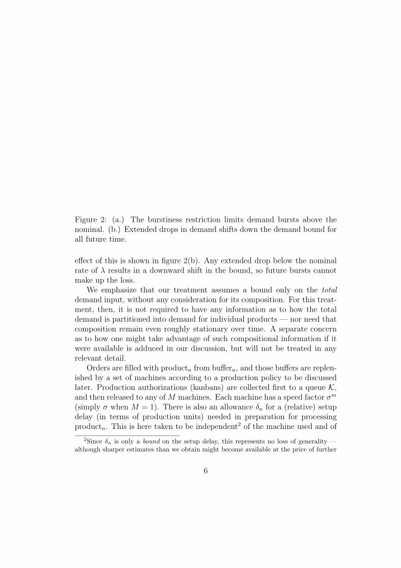
Figure 2: (a.) The burstiness restriction limits demand bursts above thenominal. (b.) Extended drops in demand shifts down the demand bound forall future time.

effect of this is shown in figure 2(b). Any extended drop below the nominalrate of λ results in a downward shift in the bound, so future bursts cannotmake up the loss.

We emphasize that our treatment assumes a bound only on the totaldemand input, without any consideration for its composition. For this treat-ment, then, it is not required to have any information as to how the totaldemand is partitioned into demand for individual products — nor need thatcomposition remain even roughly stationary over time. A separate concernas to how one might take advantage of such compositional information if itwere available is adduced in our discussion, but will not be treated in anyrelevant detail.

Orders are filled with productn from buffern, and those buffers are replen-ished by a set of machines according to a production policy to be discussedlater. Production authorizations (kanbans) are collected first to a queue K,and then released to any of M machines. Each machine has a speed factor σm

(simply σ when M = 1). There is also an allowance δn for a (relative) setupdelay (in terms of production units) needed in preparation for processingproductn. This is here taken to be independent2 of the machine used and of

2Since δn is only a bound on the setup delay, this represents no loss of generality —although sharper estimates than we obtain might become available at the price of further

6

the prior product processed. Thus, the actual processing time for productn

at machinem is τmn ≤ ρn/σ

m units of time per item of product, excludingsetup and when considering a batch of size k processed at machinem, thetotal run time, including the setup, will be bounded by (kρn + δn)/σm.

Let Vn(t) be the cumulative amount of productn released from the systemby time t, so vn(t) := ρnVn(t) is the scaled released production for productn;let v(t) be the N -vector with entries vn(t). If the level within buffern isL at time t, set xn(t) := ρn[Bn − L]; let x = x(t) be the N -vector withentries xn(t). [Note that x is necessarily bounded, as we always have xn(t) ≤ρnBn.] Similarly, let Yn(t) be the number of orders in Q at time t for productn

and let y = y(t) be the N -vector with entries yn(t) := ρnYn(t).

Example: To illustrate the meaning of the scaling factors, consider a setof metal stamping machines. In such a stamping operation, a “productionunit” could be a stroke of the stamping press. We assume each machinecan accept each part die. If machine4 is capable of 10 strokes/minute andmachine7 runs at 15 strokes/minute, then σ4 = 10 and σ7 = 15. If part 1 isproduced two at a time for its die, then ρ1 = 1/2, and τ 4

1 = 1/20, τ 71 = 1/30.

All orders and buffers are then scaled according to these production units(strokes). Thus:

• xn(t) is the number production units at time t that are required to refillbuffern to level Bn;

• yn(t) is the number of production units at time t required to empty thepresent order backlog queue, Q, of all orders it contains for productn;

• un(t) is the cumulative number of production units for productn de-manded up to time t;

• vn(t) is the cumulative number of production units corresponding tothe filled demand for productn up to time t.

As an example, suppose that up to time t, only product1 is being de-manded, so ‖u(t)‖ = u1(t). If demand for product1 up to time t is 400 units,then ‖u(t)‖ = u1(t) = 200 press strokes.

Suppose that λ = 100. Then the nominal total demand rate for allproducts is 100 production units (strokes) per minute. If ξ is 20, then over a

complication of the analysis.

7

period of 1 minute, demand could be as high as λ+ξ = 120 production units.Over 10 minutes, however, its demand could only be as high as 10λ+ξ = 1020units.

Similar examples can be constructed for other manufacturing processessuch as injection molding, extrusions, etc., where a unit of production maycorrespond to a fixed number of items. If we considered production of kits oflike parts, then instead we may have a single “product” (kit) require multipleunits of production (ρ > 1), instead of fractional units.

Note that xn(t) is the number of production units required to fill buffern

to Bn, and yn(t) is the number of production units required to fill the ordersfor productn in the backlog Q. Thus, yn(t) > 0 implies xn(t) > 0, and thesum of them can be considered a deficit of those products (in productionunits) required to have no backorders and no empty portion of the buffer forthat product.

We can thus look at the change in this deficit over time as the arrivingorders less the filled orders over the period. The basic ‘bookkeeping’ identityis then:

[x + y](t)− [x + y](s) = [u(t)− u(s)]− [v(t)− v(s)] (2.3)

for any (arbitrary) time interval (s, t] (0 ≤ s < t) and vectors indexed byproduct (n = 1, . . . , N).

Since these vectors x,y,u,v are inherently non-negative, taking the dotproduct with 1 in (2.3) gives

‖[x + y](t)‖ = ‖[x + y](s)‖+∥∥∥∥u∣∣∣ts

∥∥∥∥− ∥∥∥∥v∣∣∣ts∥∥∥∥ . (2.4)

where u∣∣∣ts

:= u(t) − u(s) is the total (scaled) units demanded over the in-

terval (s, t], and v∣∣∣ts

:= v(t) − v(s) is the total (scaled) units of production

released from the system over the interval. Let the total deficits at times sand t be the positive scalars ζs and ζt (respectively):

ζs := ‖[x + y](s)‖ = ‖x(s)‖+ ‖y(s)‖, ζt := ‖[x + y](t)‖,

Then equation (2.4) becomes simply:

ζt = ζs +∥∥∥∥u∣∣∣ts

∥∥∥∥− ∥∥∥∥v∣∣∣ts∥∥∥∥

= ζs + λ · (t− s) + ξ̃ −∥∥∥∥v∣∣∣ts

∥∥∥∥ for arbitrary intervals (s, t].(2.5)

8

Note that for each machinem our scaling of production just gives the totaldemand filled over the period as∥∥∥∥vm

∣∣∣ts

∥∥∥∥ ≥ σm · ( (t− s)− [setup time]m − [idle time]m)

and summing over m we have∥∥∥∥v∣∣∣ts∥∥∥∥ ≥ σ∗ · ( (t− s)− [setup time]− [idle time])

t− s ≤∥∥∥∥v∣∣∣ts

∥∥∥∥ /σ∗ + [setup time] + [idle time]).(2.6)

where σ∗ :=∑

m σm is the collective capacity of the set of M machines.In order that the backorder queue Q stay bounded, the cumulative ordersdemanded must not substantially exceed the orders fulfilled: over long time

intervals we must have∥∥∥∥u∣∣∣ts

∥∥∥∥ − ∥∥∥∥v∣∣∣ts∥∥∥∥ < bound. Comparing equation (2.6)

with (2.1), we get the necessary constraint that this collective capacity σ∗

must exceed the total demand rate λ:

σ∗ > λ where σ∗ :=∑m

σm. (2.7)

In this paper, we consider several protocols which dictate when machineswill produce a product and how many will be produced in sequence. A proto-col thus specifies how the queue K of production authorizations is maintainedand how it determines the activity of the machines (processors). A key con-cept of interest is whether our protocols will guarantee a bounded orderbacklog Q, and further, whether that order backlog will eventually emptyand remain empty.

Definition 1 A protocol is stable — for given load scalings ρn , speeds σm ,and configuration (buffer sizes) — if Q remains bounded (i.e., ‖y(t)‖ remainsbounded for all t) for arbitrary initial state, subject only to the burstiness ar-rival constraint equation (2.1), and the capacity constraint (2.7). A protocolis uniformly stable if the bound on the queue size ‖y‖ depends only on theinitial queue size, uniformly for all admissible input.

Definition 2 A protocol is clearing if, for arbitrary initial state and ad-missible input as above, Q necessarily empties; it is strongly clearing if, in

9

addition, Q stays empty from some time on. A protocol is uniformly clear-ing if there is some bound on the time to clearing, depending on the initialqueue size, but uniform for all admissible inputs; it is uniformly stronglyclearing if this also holds for the time until the queue remains clear.

Theorem 1 Every stable protocol is uniformly stable. Similarly, every clear-ing protocol is uniformly clearing and every strongly clearing protocol is uni-formly strongly clearing. Finally, clearing protocols are necessarily stable andso are uniformly stable.

Proof: As this theorem is somewhat tangential to our principal inter-ests we only sketch the arguments.(stable ⇒ uniformly stable) Suppose not. Then each trajectory (i.e.,sequence of states3) is bounded, but there is some sequence {yν(·)} of suchtrajectories for which ‖yν(tν)‖ ≥ ν for suitable times tν . Without loss of gen-erality we can assume there are no state repetitions (at least, earlier than tν)in any of the trajectories under consideration here: else one can skip the in-tervening segment of the trajectory (noting that our definition of ‘protocol’requires that the ‘reduced’ trajectory must again be admissible). By a diago-nal argument one can find a subsequence of trajectories with common initialsegments of increasing length: all trajectories agree up to the N -th eventfrom some point ν(N) on. This determines a common ‘limit trajectory’,which must also be admissible and so should be bounded by the assumedstability. On the other hand, it cannot be bounded since the absence of rep-etitions ensures a bound on the number of steps until ‖y‖ ≥ c for any c (asthere are only finitely many distinct states with ‖y‖ ≤ c). This contradictionshows the existence of a uniform bound for fixed initial conditions whence,since there are only finitely many initial conditions satisfying any bound, wehave uniform stability.

(clearing ⇒ uniform clearing) Again, suppose not. Then there wouldbe a sequence of trajectories with increasing times to clearing and increas-ing number of arrivals before clearing4 Again by a diagonal argument, we

3Without loss of generality we need consider only those evolutionary histories for whichthe input is close enough to the rate λ of (2.1) that (uniformly) one can work with sequencesof orders and states (buffer and queue contents) without explicit regard to times.

4If there would be a long enough interval without input, then (as our definition of‘protocol’ ensures the system will not idle for long when the queue Q is not empty) thesystem will clear. This clearing can only be delayed if input continues.

10

can extract a subsequence with increasingly long common initial segments(again determining a ‘limit trajectory’) and with increasingly long periodsto clearing. The limit trajectory is necessarily admissible but never clears —contradicting the assumed clearing property.

(uniform clearing ⇒ uniform stability) Over a uniformly boundedtime before clearing, the condition (2.1) bounds arrivals so the possible queuelength is bounded.

(strong clearing ⇒ uniform strong clearing) The proof is by thesame kind of diagonal argument as above.

In this paper we consider two protocols: the Signal Kanban protocol (intwo variations) and the Pattern Production protocol.

For the Signal Kanban protocols we let Rn (with 0 ≤ Rn ≤ Bn) be a‘reorder level’ such that kanbann is to be transmitted to K to ‘order’ produc-tion by the machine(s) to replace the ‘deficit’ when the buffer level gets downto Rn; i.e., the kanban is transmitted when xn reaches bn := ρn[Bn−Rn] ≥ 0.Each kanbann is then transferred back to buffern when the corresponding pro-duction run (consisting of ‘setup’ plus actual processing time) is completed.

There are two common variants of the Signal Kanban protocol:

• fixed-batch: In the fixed-batch version of a Signal Kanban, the pro-duction authorization is for a fixed lot size (scaled) of exactly bn. Thisis the version of Signal Kanban discussed by Monden [9], and seemsto be most common in industry. This is the same as the reorder-point(“two-bin”) methods in inventory theory. We normally assume prod-uct is transferred to the appropriate buffer immediately (continuouslyduring processing), but we note an alternative subvariant with productdelivery of the entire batch made at completion of the production run.

• fixed-fill: In the fixed-fill protocol, the signal kanban authorizes pro-duction to fill the buffer, i.e., up to Bn. The production runs may beof different lengths depending on the demand for this product fromthe time of issuance of the kanban authorization until completion ofthe run with the buffer filled. Queuing delays in K due to other pend-ing authorizations make the initial buffer level at the start of the runvariable, but it is no higher than the reorder level, so bn represents aminimum batch size. The disadvantage of this system in practice isthat the variable run lengths require monitoring the buffer levels while

11

running, as opposed to the simpler fixed-batch scheme. However, frominitial simulation studies, the fixed-fill appears to have a better behav-ior [5]. It is interesting to note that in the limit where the buffer levelsbecome continuous variables instead of discrete, the “fixed-fill” vari-ant is equivalent to the “switched arrival” system shown to be chaotic(the behavior is highly sensitive to initial conditions, and it is highlyunlikely that the system will settle into a periodic pattern) by Chase,Serrano, and Ramadge [3].

We emphasize that for either variant the authorized production run will havea (scaled) ‘batch size’ at least bn, i.e., bn is the minimum run length. Signalkanbans are discussed in more detail in the next section.

For the Pattern Production protocols we have a specified ‘cycle’ ofkanbans in fixed sequence (n(1), . . . , n(J)) with every index n included atleast once in the cycle. Each of these kanbans is transferred to the rear endof the queue K as soon as the corresponding production run is initiated. Forthe special case where each product appears exactly once in the pattern andthere is only one machine, this is equivalent to a Signal Kanban system withRn = Bn. Thus, an authorization is released immediately upon the filling ofthe buffer. Pattern Production protocols are examined in Section 4.

3 Signal kanbans: amortizing batch sizes

We wish to consider a set of M machines, working collaterally (in parallel) toserve a common set of buffers with a common input stream to the queueQ. Ina Signal Kanban system, we associate a reorder point Rn with each buffern.Whenever the buffer level falls to this level (corresponding to xn reachingbn := ρn[Bn−Rn] > 0), then a production authorization (kanban) is releasedto the kanban queue K to replenish productn.

The specification of a minimum run length is the substantial point ofthe Signal Kanban protocol in the presence of setup times: we will chooseeach Rn (and so bn) so as to amortize the setup times. Choosing α > 1, setσ′ := σ∗/α. For any production run of length b (in terms of scaled product),the time taken by the run, including setup time, will then be bounded by(b + δn)/σ. If we would know, by the specification of the minimum, thatb ≥ δn/(α − 1), then this total run time would be bounded by b/σ′ and σ′

becomes a reduced ‘effective capacity’ for the set of machines, subsuming

12

consideration5 of setup times.We use the obvious specification of queue dynamics: If a production run

is in progress, it continues according to the variant selected; in each case theminimum run length is bn. When the machine finishes such a run, it returnsthat kanban to its buffer and then immediately begins the new run associatedwith the kanban now at the head of K, if any. If K is empty, then the machineidles until a kanban arrives to K and that run is initiated. A production run,once initiated, consists of the setup, followed by the actual processing; itis possible that two (or more) consecutive production runs may involve thesame product6 and in that case we assume (or, as an alternative variant, maynot!) that the setup time is omitted or reduced for all but the first of theseruns. We allow the variants of the Signal Kanban protocol regarding ‘fixedbatch size’ or ‘fill the buffer’ as above. Our analysis will accommodate anyof these variants without distinction, assuming the capacity condition (2.7).

The specification of system dynamics requires some further considerationwhen M > 1: How should one handle the possibility of partial idling (some,but not all, of the machines being active at t)? If we accept this as a possibil-ity while imposing the capacity condition in the form (2.7), then partial idlingmeans that the battery of machines may be operating below its collective ca-pacity σ∗ and it should not then be surprising that stability might fail.7 To

5It will be important to take advantage of the strict inequality in the capacity condi-tion (2.7), to choose α < σ∗/λ so σ′ > λ. Otherwise, one easily sees that with run lengthsshort enough that the capacity condition now fails — i.e., if σ′ < λ in (2.7) — then thesystem cannot be stable: too high a proportion of the time would be taken up by thesetups and the effectively reduced capacity becomes inadequate to keep up with demandinput.

The significance of our choice of α > 1 is that a larger α (farther from 1) means smallerbatch sizes and requires smaller buffers – but somewhat limits the load which could behandled, corresponding to a possible increase in λ.

6This can happen if there is an intervening idle period or if we are working with afixed batch size and, when the kanban is returned to the buffer, the buffer level is alreadyat or below the reorder level (due to further demand since the kanban was previouslytransmitted to K) and the kanban is then immediately retransmitted to K. Of course, thisalso assumes that no other kanban is transmitted between these occurrences.

7Consider the scenario (say, in the ‘fill the buffer’ variant) in which, from some mo-ment on, the external demand stream becomes entirely composed of orders for some oneproductn̄. The kanbann̄ has initiated a production run for productn̄ (e.g., at machinem̄)and, after a while, all the other machines would be idle while machinem̄ works at speed σm̄.The capacity condition (2.7) permits arrival of orders at a (scaled) rate λ. Although λ < σ∗

by assumption, it remains possible that λ > σm̄ — the input rate dominating the pro-

13

obtain a positive result we must include some ‘assistance rule’ in extendingthe protocol to the collateral case, rather than having a kanban exclusivelyassign a production run to a single one of the machines. We will think ofK as consisting of two disjoint parts: Ka := {those kanbans in K alreadyassigned to some machine (so a production run is already in progress)} andK0 := {those kanbans in K awaiting assignment}. A machine, on completinga production run, is assigned a new run from K0 if that is nonempty andotherwise initiates a run ‘in assistance’ from Ka (e.g., the first, although thischoice does not affect our argument); if K0 and Ka are both empty, then thesystem is (entirely) idle with K empty. While we have described a particularversion of the assistance rule for definiteness, we will really need only twoproperties of this for our proof:

• When the system is idle each buffer must be above its reorder level.

• When several machines participate in a compound production run, wewill have a setup time for each (with the possibility of omitting this ap-plicable on a machine-by-machine basis), but cannot have more than Msuch altogether for any single such run.

It would be convenient to have also the property that all machines involvedin a compound production run finish simultaneously (with a ‘priority rule’to determine order of subsequent assignment). In this situation, we wouldbe concerned with the possibility of a machine assigned to to the productionof a part being within a setup process when the production is completed bythe others machines. In the case of ‘fixed batch size’ this would necessarilybe predictable and we modify the assistance rule to assign this machine tothat run, but not have setup actually performed — although the time untilthe run is completed might be counted as setup time, rather than as idling.In the case of ‘fill the buffer’ this predictability might fail and we will allowfor this possibility of incomplete setup in our analysis.

Theorem 2 Consider a Signal Kanban protocol as described above for col-lateral operation of a set of M machines satisfying (2.7). We choose α so1 < α < σ∗/λ and suppose the reorder levels Rn ≥ 0 are set so that

bn := ρn[Bn −Rn] ≥ Mδn/(α− 1) (3.1)

duction rate so the system cannot keep up, i.e., instability. The problem obviously is thatσ∗ truly represents system capacity only in that multiple machines can combine to handlethe load and, for our setting, this must be allowed to hold even when the composition ofthe load might be concentrated on a set of products smaller than the number of machines.

14

for each n. The following statements can then be made for either the fixedbatch or fixed fill variants of the protocol:

1. The protocol is uniformly stable.

2. The protocol is uniformly clearing: the maximum length of any activeinterval (s, t] is at most

Tmax :=ζs + ξ

σ∗/α− λ(3.2)

where we note that, except initially, ζs < btot :=∑

n bn.

3. If the buffer sizes are large enough [see (3.5) and, e.g., (3.7), below],then the protocol is (uniformly) strongly clearing.

Proof: Fix a time s at which the system becomes active (i.e., eithers = 0 or s ends an idle period. Our protocol description ensures that ifany machine is ‘idle’ then all machines are idle and Q is empty so y = 0and ‖x‖ < btot :=

∑n bn, whence ζs < btot when s 6= 0 here. We then fix

an interval (s, t] during which the system remains active without any idling.Indexing production runs (whether simple or compound) during this intervalby ν, we have

σm(t− s) ≤∑ν

[b + δ]mν

where [b, δ]mν here represent the shares of (scaled) production and setup,respectively, for runν within (s, t] by machinem and we have no idle time toconsider. Summing over m we get

σ∗(t− s) ≤{∑

ν

′+∑ν

′′}

[b + δ]ν

where we have separated the sum into∑′, consisting of those (complete) runs

occurring entirely within (s, t], and∑′′, the remaining (partial) runs: note

that this latter sum consists of those runs not yet finished by t since ourchoice of s ensures that none of the runs involved here is incomplete because

it was initiated before s. We then have{∑′

+∑′′}

[b]ν =∥∥∥∥v∣∣∣ts

∥∥∥∥.For each of the complete runs in

∑′ we know that b ≥ bn with n =n(ν) and that we have at most one setup time for each of the machines,

15

whence [δ]ν ≤ Mδn. Thus, using (3.1), we have [b + δ]ν ≤ α[b]ν for each ofthese runs. To estimate

∑′′ we note that there can be at most M machinesinvolved in those runs in process at time t so, altogether, their setup ‘costs’can be at most Mδmax with δmax := maxn{δn}: i.e.,

∑′′[δ]ν ≤ Mδmax.Combining these gives, since α > 1,

σ∗(t− s) =

{∑ν

′+∑ν

′′}

[b + δ]ν

≤ α∑ν

′[b]ν +

{Mδmax +

∑ν

′′[b]ν

}≤ Mδmax + α

∥∥∥∥v∣∣∣ts∥∥∥∥ .

(3.3)

Using (2.5) in (3.3) gives

ζt ≤ ζs + ξ + (λ/σ∗)Mδmax −(

1− λα

σ∗

)∥∥∥∥v∣∣∣ts∥∥∥∥

and, as λα/σ∗ < 1 by assumption, the last term above can be omitted andwe have

ζt ≤ ζs + ξ + (λ/σ∗)Mδmax. (3.4)

Since ζt := ‖[x+y](t)‖ and ζs is uniformly bounded (either ζ0 or < btot), thisshows that the protocol is uniformly stable, so statement 1 of this theoremis proved.

Next we determine the maximum time the system can be busy withoutreturning to idle. Taking t above to be the end of the active interval, we have∑′′ empty so we can omit the Mδmax term of (3.3). From (2.5) we then have

ζt ≤ ζs + λ · (t− s) + ξ̃ − (σ∗/α) (t− s).

Solving for (t− s) and recognizing that ζt ≥ 0, we arrive at

(t− s) ≤ ζs + ξ

σ∗/α− λ,

which gives us the desired bound (3.2).To prove result 3 of the theorem, our simplest argument is to note that

xn̄(τ) < bn̄ for τ within any idling period while for τ in a non-initial activeperiod (s, t] we have, as s ≤ τ ≤ t ≤ s + Tmax,

xn̄(τ) ≤ xn̄(s) + [λ(τ − s) + ξ] < bn̄ + λTmax + ξ

16

with Tmax computed as in (3.2) using ζs < btot. Clearly, if the buffer size Bn̄

is set large enough that

ρn̄Bn̄ ≥ bn̄ + ξ +btot + ξ

σ∗/α− λ, (3.5)

then this buffer could not empty as would be necessary to have an order forproductn̄ at the head of the backlog queue Q. If this holds for every n̄, thenQ must remain empty since no order could be at its head.

While proving statement 3, this universal and explicit estimate (3.5)is clearly unreasonably pessimistic, since an input stream maximizing thelength of the active interval as in (3.2) would not be expected to maximizexn̄(τ) at τ = t.

We would prefer a sharper estimate of the lower bounds for the buffersizes which will ensure strong clearing. For the general case with M > 1 thesituation is rather complicated, as one must consider combinatorial aspects ofthe machine assignments and assistance to obtain a ‘good’ bound for xn̄(τ)in an active period. We will seek to obtain such an estimate only underthe additional assumption8 that it requires all the machines to keep up withdemand arriving at the maximal rate of (2.1) — i.e., with (2.7) we wouldhave

σ∗ − σm < λ < σ∗ ∀m. (3.6)

We also continue to assume that (3.1) holds for each n. A simplifying con-sequence of (3.6) is that a time τ at which xn̄(τ) attains its maximum mustimmediately precede a period of production of productn̄ with assistance byall machines so all production runs during (s, τ ] for products n 6= n̄ arecompleted and for such n we have9

[production]n = Knbn with Kn :=

⌊xn(s) + [input]n

bn

⌋.

We note here that the expression (αλ/σ∗)Knbn − [input]n is then maxi-mized (least negative) when xn(s) is as large as possible (for s− ending an

8This holds automatically for the single machine case M = 1 and we note that therequirement we obtain will be sharp in that case. When M > 1 it seems possible thatsome slight further improvement might still be achieved by a more detailed analysis (e.g.,to show that one typically has one, rather than M setups for each production run), butwe do not pursue this and consider (3.7) sufficiently sharp.

9We also write [production]n̄ = Kn̄bn̄ with Kn̄ ≥ 1, although Kn̄ will not, in general,be an integer.

17

idle period: xn(s) = bn−ρn) and the input is just what is needed to trigger arun (i.e., [input]n = ρn so Kn = 1) for n 6= n̄. Further, each of these completeruns is amortized so

[production + setup time]n6=n̄ ≤ α[production]n6=n̄ = α∑n6=n̄

Knbn

while, as Kn̄ need not be an integer, we similarly have

[production + setup time]n̄ ≤ αKn̄bn̄ + δ̃(δ̃ ≤ δn̄

).

Note that (2.6) then gives

τ − s ≤ [production + setup time]/σ∗ ≤(α∑n

Knbn + δ̃

)/σ∗.

At this point we are ready to bound xn̄: using the observations aboveand (2.1), we have

xn̄

∣∣∣τs

= [input]n̄ − [production]n̄

= [input]− [input]n6=n̄ −Kn̄bn̄

≤ λ(τ − s) + ξ − [input]n6=n̄ −Kn̄bn̄

≤ (λ/σ∗)

(α∑n

Knbn + δ̃

)+ ξ − [input]n6=n̄ −Kn̄bn̄

= ξ + (λ/σ∗)δn̄ − (1− (αλ/σ∗)Kn̄bn̄ +∑n6=n̄

((αλ/σ∗)Knbn − [input]n)

≤ ξ + (λ/σ∗)δn̄ − (1− (αλ/σ∗)bn̄ +∑n6=n̄

((αλ/σ∗)bn − ρn)

xn̄(τ) = xn̄(s) + xn̄

∣∣∣τs≤ bn̄ − ρn̄ + xn̄

∣∣∣τs

≤ ξ + (λ/σ∗)δn̄ +∑n

((αλ/σ∗)bn − ρn) .

Thus, as earlier for (3.5), we see that requiring

ρn̄Bn̄ > ξ +λ

σ∗ δn̄ +∑n

(αλ

σ∗ bn − ρn

)(3.7)

for each n̄ is sufficient, in the context of (3.6) and subject to (3.1), to ensurestrong clearing.

18

Example: To illustrate the above results, consider a manufacturingfacility with two “machines”, with scaled production rates of σ1 = σ2 = 9units/min. Our machines produce six products with scaled setup for eachproduct of δ1 = δ2 = δ3 = δ4 = 80 (production units) and δ5 = δ6 = 40.These represent worst-case setups – when switching between certain pairsof products, common settings between particular products may reduce thesetup effort. In our example, a production unit equals an item of product,so ρi = 1 for 1 ≤ i ≤ 6. For the production rates given, the average setuptime on machine1 thus corresponds to 8.9 minutes.

Suppose that we have a demand of λ = 15 units/minute. The collectivecapacity is then σ∗ = σ1 + σ2 = 18 units/minute, and the utilization isλ/σ∗ = 83.3%. The parameter α must be chosen between 1 < α < σ∗/λ =1.2. First let us consider the case where α := 1.15. In this case, by equation3.1, b1|α=1.15 ≥ 1067 units, which would correspond to at least 71 minutesof supply if demand swings entirely to product 1. If demand did swingentirely to one product, then the two machines must both eventually help,since the rate of demand would exceed the capability of either machine byitself. Note that regardless of the demand, each production run will take(bn + δn)/σ1 = 127 minutes if run on just one machine.

Note that product6 setup is only δ6 = 40. For this, b6|α=1.15 ≥ 533.3units. This is significantly lower than for product1, illustrating (as we wouldexpect) that the minimum scaled buffer size (and thus the investment ininventory) is reduced proportional to scaled setup time δi.

The parameter α must lie between 1 and σ∗/λ. Moving α closer to oneeffectively limits the load by forcing larger batches and less frequent setups.Thus, it in effect reserves capacity that could cover a potential long-termincrease in λ. To illustrate the effect of decreasing α, suppose now thatα = 1.05. Then b1|α=1.05 ≥ 3200 units.

The buffer bounds calculated above ensure that the system will be stableand the backlog will be bounded. However, typically we are more concernedwith preventing a backlog from occuring. Assume that our burstiness boundξ is 5 units. From above, we have

∑6i=1 bi|α=1.15 ≥ 5336. Then from equation

3.7, we have the buffer size for product1 must be

ρ1B1|α=1.15 > 5179.3

Thus, if the buffer for product1 is at least 5180 parts deep (approximately5.75 hours of maximum demand), then it is sufficiently deep such that no

19

part shortage will occur, even under the “worst case” situation of all kanbansbeing released simultaneously. We should emphasize that this this value isprimarily due to the term

∑6i=1 αλbi/σ

∗, which corresponds to replenishingwhen all products are at their reorder points simultaneously — possible,although unlikely.

4 Pattern production

We continue to consider a set of M machines working collaterally (in parallel)to serve a common set of buffers with a common input stream to the queue Q.In this section we wish to show stability and strong clearing for PatternProduction protocols, such as simple ‘Round Robin’, in which there is apredetermined cyclical specification of the sequencing of production runs. Ingeneral the system will be continuously active, since the queue K will alwayscontain the full (cyclical) set of kanbans. However, there will be no positiveminimum for the batch sizes and the problem is to verify that the setuptimes are amortized by an automatic adjustment of the batch sizes so thesetup times just fill the capacity gap (σ∗ − λ). While there are no ‘reservelevels’ to specify for these protocols, it will be necessary to require lowerbounds on the buffer sizes.

Two comments are in order here as to the precise specification of theprotocol. First, much as in our description of the Signal Kanban protocols,we wish to allow (as one alternative possibility) that we omit the setup whenit is clearly unnecessary: here, if the buffern(j) is already completely full whenone comes to the j-th kanban of the cycle. Conceivably there might be someinterval, necessarily with no external demand input, during which all buffersremain full and, in the no-setups variant, we do not take this as meaning thereare infinitely many (totally degenerate) ‘cycles’ in no time, but simply movethe ‘head’ of the kanban queue to the kanban for the next arriving order,with some selection rule or arbitrary choice if that might be ambiguous dueto multiple occurrence of this n in the cyclical pattern. Second, we note— by the same logic as preceding Theorem 2 — that ‘assistance’ may benecessary. However, this is now implicit in what we have described of theprotocol without introducing a special ‘assistance rule’: if machinem becomesavailable and the next kanban is one for which a production run is alreadyunder way with10 that buffer not yet full, then machinem initiates an ‘assisting

10It is almost necessary that the buffer be not yet full if a production run is under way,

20

run’ for the same product.

Theorem 3 Consider a ‘Pattern Production’ (cyclical) protocol for collateraloperation of a set of M machines satisfying (2.7). We assume that all thebuffer sizes have been set so

bn := ρnBn > ζ∗ :=(λ/σ∗)∆∗

1− λ/σ∗

with ∆∗ := M∆ + (M − 1)δmax ∆ :=∑

j δn(j).(4.1)

Then

1. The protocol is uniform clearing and stable. Moreover, for M = 1 thesame conclusion holds even if we admit one exception to (4.1).

2. If the buffer sizes satisfy the stronger condition

bn > ζ∗ :=2− λ/σ∗

1− λ/σ∗ (λ/σ∗)∆∗ + ξ, (4.2)

then the protocol is uniform strongly clearing.

Proof: The key to the proof will be the property:

If j is the first time n = n(j) occurs, then the production of

productn in the j-th run of the cycle must be at least xn(s).(4.3)

This property is clear when M = 1, but our first concern here is to determinea suitable replacement for it, since (4.3) is no longer valid, as stated, in themore general context. The difficulty is that, unless xn(s) = 0, a productionrun for productn(j) will be initiated, but need not now terminate within thecycle: this is, after all, the reason we have found it necessary to introduce thenotion of ‘assistance’. Hence the desired lower bound on production in (4.3)may fail in considering a single cycle.

but not quite: a first machine might initiate a run of productn and then a second machineinitiate assistance, after which it is possible that a third machine will become availablewith this again the ‘next kanban’ after the first machine has already filled the buffer, butwhile the second machine is still in its setup time, so the run remains ‘under way’.

21

Instead, we will analyze production over an interval (s, t] consisting ofseveral consecutive cycles, defining such intervals by requiring that each pro-duction run associated with a ‘first occurrence’ j of productn(j) in the firstcycle of the interval must have terminated by the end of the interval withbuffern(j) filled. Then (4.3) holds in the present setting with ‘cycle’ replacedby ‘interval’. Summing this over j — i.e., over n, since each n occurs for itsfirst time exactly once in (s, t] — we see that we always have∥∥∥∥v∣∣∣ts

∥∥∥∥ ≥∑n

xn(s) = ‖x(s)‖. (4.4)

Excluding the possibility that the input stream of orders is finite, we havea well-defined sequence of intervalsν for ν = 1, 2, . . . with ν →∞ as t →∞.We let tν denote the completion time of the ν-th interval (with t0 = 0) andconsider (s, t] = (tν−1, tν ]. Here (2.6) becomes

σ∗ · (t− s) =∥∥∥∥v∣∣∣ts

∥∥∥∥+ ∆̃ (∆̃ = ∆̃ν := [total of setup times])

since no time is occupied by idling.To obtain an estimate for the [total setup time]ν =: ∆̃ν associated with

such an interval, we first observe that one of our ‘intervals’ can consist of atmost11 M cycles. It is then clear that the setup times associated with allruns (including ‘assisting runs’) initiated within the cycles comprising theintervalν cannot exceed M∆. We do note, however, the possibility that atthe time tν−1 at which the intervalν began, perhaps as many as (M − 1) ofthe machines were involved in doing setups and to estimate ∆̃ν we must alsoallow for these. Altogether, ∆̃ = ∆̃ν ≤ ∆∗ with ∆∗ as in (4.1) and using thisin (2.5) gives the recursive identity

ζt = ζs − (1− λ/σ)∥∥∥∥v∣∣∣ts

∥∥∥∥+[(λ/σ)∆̃ν + ξ̃ν

]. (4.5)

11To see this, consider any j which is a first occurrence of n = n(j) in the cycle patternand the production run associated with this, starting in the first cycle of the interval.If this run has not terminated (with buffern filled) by the occurrence of j in the secondcycle of the interval, then a second machine will initiate an assisting run of the sameproductn. By the occurrence of j in the M -th cycle of the interval — if the interval hasextended this long because this run remains incomplete — all M machines will be workingon processing this same productn so the M -th cycle could only end after the completionof this compound run. (As before, we note that the capacity condition (2.7) ensures thatthis must eventually happen.)

22

We now assume that (4.1) holds for all n and distinguish two cases forthe system state at the time s = tν−1: either there is no backlog at that time(i.e., Q is empty and y(s) = 0) or there is a backlog (i.e., Q is nonempty).

Case 1: If the queue Q(s) is empty so y(s) = 0, then ζs = ‖x(s)‖ and wemay use (4.4) in (4.5) to get

ζt ≤ (λ/σ)ζs +[(λ/σ)∆ + ξ̃ν

]. (4.6)

[So far, this has used no assumption about the buffer sizes.]

Case 2: If, however, Q(s) is nonempty, we denote by n̄ the index of theitem at the head of that queue. This is possible only if the buffern̄ is empty

so xn̄(s) = bn̄ and we note from (4.4) that this gives:∥∥∥∥v∣∣∣ts

∥∥∥∥ ≥ bn̄. Using this

in (4.5) gives

ζt ≤ ζs − (1− λ/σ)bn̄ +[(λ/σ)∆̃ν + ξ̃ν

]≤ ζs + ξ̃ν − c

(4.7)

wherec := min

n{(1− λ/σ∗)bn − (λ/σ∗)∆}. (4.8)

The assumption (4.1) just ensures that c > 0.

Now, for M = 1 (so our intervals are simple cycles), consider the modi-fications needed if we admit a single exception to (4.1). Without loss ofgenerality we may assume the exception is for n = 1 and that we have havetaken the ‘beginning’ of the cycle there, so j(1) = 1. We modify the casedistinction to consider also the state at the time s′ at which the first pro-duction run of cycleν (for product1) terminates: Case 1 now corresponds to“Q(s′) is empty” (rather than to “Q(s′) is empty” as earlier) and Case 2corresponds to “Q(s′) nonempty.” More specifically, Case 1 now includesboth Case 1′ with Q also empty at s (as above, with the identical analy-sis) and also Case 1′′ where Q(s) is nonempty and n̄ = 1 but Q(s′) is empty(thus, Q(s) contained only product1, and no new backorders entered Q whileprocessing product1 over the interval (s, s′]). For Case 2, we now either haven̄ 6= 1 so (4.1) applies and the analysis is as before, or we have n̄ = 1 withQ(s′) nonempty (thus, backorders entered Q during the production run ofproduct1 over the interval (s, s′]). In the latter subcase the index of theitem at the head of the queue at s′ will be n̄′, necessarily with n̄′ 6= 1 so(4.1) will apply and, since this n̄′ must occur later in the cycle than n̄ = 1with j(n̄) = 1, we note that cycleν contains a production run for productn̄′

23

starting with buffern̄′ empty so∥∥∥∥v∣∣∣t

s

∥∥∥∥ ≥ bn̄′ .

Either way, Case 2 gives ζt ≤ ζs + ξ̃ν − c, i.e., (4.7), with c > 0 nowdefined by taking the minimum over n 6= 1 in (4.8). For Case 1′′ all of y(s)will have been subtracted from the respective buffers by the time s′ to givey(s′) = 0 and we note that the production of product1 during the first runof the cycle must be at least x1(s) + y1(s) and the production of each otherproduct (n 6= 1) occurs subsequent to s′ and so must be at least xn(s′) ≥

xn(s) + yn(s): altogether we must have∥∥∥∥v∣∣∣t

s

∥∥∥∥ ≥∑n [xn(s) + yn(s)] = ζs as

earlier so, for either subcase, we still have (4.6) for Case 1.

A first consequence of (4.7) is then that any backlog occurring must even-tually clear: one can only have finitely many12 consecutive cycles in Case 2.Setting

k(ν) := [number of cycles in Case 1 through cycleν ],

we note that (4.1) ensures that: k(ν) →∞ as ν →∞. We now observe that(4.6) and (4.7) give

ζt ≤ (λ/σ∗)k(ν)ζ0

+[1− (λ/σ∗)k(ν)

] (λ/σ∗)∆

1− λ/σ∗

+ν∑

µ=1

(λ/σ∗)k(ν)−k(µ)ξ̃µ

(4.9)

for ν = 0, 1, . . .. This is trivially true for ν = 0 with k(0) = 0, and thenproceeds easily by induction — using for this, as appropriate, either (4.6)with k(ν + 1) = k(ν) + 1 or else (4.7) with k(ν + 1) = k(ν).

For an arbitrary time τ (falling in the (ν + 1)-th cycle, so tν ≤ τ ≤ tν+1)the same analysis which gave (4.5) can also be applied to the time interval(tν , τ ], giving13

ζτ ≤ ζt +[(λ/σ∗)∆∗ + ξ̃τ

](4.10)

12From (4.7) we have: ζtν+k≤ ζtν−1 + ξ̃ − kc if intervalν through intervalν+k were

Case 2 intervals (with ξ̃ corresponding to the entire concatenated time interval so ξ̃ ≤ξ). With c > 0 this would contradict the positivity of ζtν+k

for large enough k, greaterthan (ζs + ξ)/c.

13In (4.10) we could replace the bound on setup time within (s, τ ] by summing δn(j)

only over those setups actually occurring by τ , but we use ∆∗ as in (4.1) for simplicity.

24

and combining this with (4.9) gives

ζτ ≤ (λ/σ∗)k(ν)ζ0 +(2− λ/σ∗)(λ/σ∗)∆

1− λ/σ∗ + Ξτ

with Ξτ := ξ̃τ +ν∑

µ=1

(λ/σ∗)k(ν)−k(µ)ξ̃µ.(4.11)

To estimate Ξτ , begin by defining

Ξ̃κ := ξ̃τ +ν∑

µ=κ

ξ̃µ = ‖u(τ)− u(tκ−1)‖ − λ · (τ − tκ−1)

βκ := (λ/σ∗)k(ν)−k(κ) (βν+1 = 1)

for κ = 1, . . . , ν +1. Note that each Ξ̃κ ≤ ξ by (2.2) and that ξ̃µ = Ξ̃µ− Ξ̃µ+1

for µ = 1, . . . , ν with ξ̃τ = Ξ̃ν+1. Further, since k(·) is nondecreasing, wehave βκ ≥ βκ+1 for each κ. Simplifying the summations by setting Ξ̃ν+2 := 0and β0 = 0, we may use Abel’s formula for summation by parts to get

Ξτ = −ν+1∑µ=1

βµ

[Ξ̃µ+1 − Ξ̃µ

]=

ν+1∑µ=1

[βµ − βµ−1] Ξ̃µ

≤ν+1∑µ=1

[βµ − βµ−1] ξ = [βν+1 − β0] ξ = ξ.

This shows that Ξτ ≤ ξ for all τ , which gives uniform stability in view of(4.11) — i.e., subject to (2.7), (4.1). Asymptotically,

ζτ ≤ (λ/σ∗)k(ν)ζ0 + ζ∗ → ζ∗ (as τ →∞)

since then k(ν) →∞.Finally, if (4.2) holds — so a fortiori (4.1) holds — then, from some time

on (such that k(ν) is large enough to make the first term on the right of(4.11) negligible) one has ζτ < bn for every n. Thus, as each xn̄(τ) ≤ ζτ , nobuffern̄ can be empty so no n̄ can index the item at the head of the queue.This means that Q must then be empty — which is just the strong clearingproperty.

Example: To illustrate our results for a pattern production system, weconsider the same example as at the end of section 3. From equation 4.1,

25

bn := ρnBn > ζ∗ = 4400 production units. This equates to 4.8 hours ofmaximum demand for the product.

To ensure strongly clearing, from equation 4.2, bn > ζ∗ = 5138.3. Thus,if the buffer is at least 5139 production units (products) deep, then we areassured that there will be sufficient inventory to prevent backlogs even underchanges in demand mix and under demand burstiness.

Now, suppose that the sequence pattern of production can be chosento take advantage of similarities of adjacent products in the sequence, thusreducing the setup times.14 In particular, suppose the resulting savings insetups due to sequencing leads to ∆′ = 200 and δ′max = 60, which thengives ζ∗ = 2300 as a bound to ensure stability, and ζ∗ = 2688.3 as a boundto ensure strongly clearing and thus no backlogs. This illustrates that ouranalysis can be applied to cases where the production sequence is carefullyselected to reduce setup times.

5 Discussion

In this paper, we have examined several variants of production protocols formanufacturing systems where setups can have a significant impact on ca-pacity. Each protocol examined is a pull protocol, so production is directlyin response to prior and current consumption (demand). We considered sys-tems where the demand is unknown. A maximum average long-term demandrate is assumed known, but the demand can exceed this bound subject toa ’burstiness’ constraint. There are no assumptions on the distribution ofthis demand or the burstiness among the different products being produced.We examined variants of the Signal Kanban systems and Pattern Productionsystems, for the situation of single machine and parallel machines.

Our focus in this paper was on determining whether these protocols werestable and strongly clearing. A protocol is stable if the backorder queueremains bounded, and is strongly clearing if the backorder queue eventuallyempties and remains empty thereafter. For each of the policies we considered(subject to a capacity constraint), conditions on the buffer sizes were found inorder to ensure that the policies would be both stable and strongly clearing.

14This is very reasonable when M = 1 when the sequence of products in the patterndirectly determines the sequence of products on the machine. Using the sequence toreduce setups when M > 1 seems less reasonable, but we nonetheless continue with ourmulti-machine example.

26

We should emphasize that we assumed no structure to the distributionof demand among products, or of the distribution of the burstiness amongproducts. As such, the bounds that were determined for setting buffer sizesand reorder points would be conservative in practice. In lean manufactur-ing, where pull production methods are commonly used, there is a strongemphasis on heijunka, leveling demand over time and among products. Thishas an impact on our results in two ways. First, there would be a consciouseffort to minimize the burstiness ξ. Secondly, for each productn, we wouldhave a maximum demand rate of λn ≤ λ such that λ ≤ ∑N

n=1 λn ≤ Nλ. Thedevelopments in this paper have considered the worst case where λn = λ forall n, but reducing each λn to more accurately reflect knowledge of demandwould reduce the buffer level bounds accordingly.

There are several directions for continued work on these protocols. First,it would be useful to determine better buffer sizes and reorder points whenknowledge of the distribution of demand among products is known. A seconddirection for investigation is the performance of the protocols. Average inven-tory is one performance measure of importance in many industries. Yang [17]used simulation to compare the average inventory of a fixed-fill signal Kan-ban system (a reorder point policy) with a model intended to approximatetraditional Kanban methods, but which in fact resembles the behavior of apattern production system (specifically, in his model, inventories are alwaysreplenished to their maximum level, and an authorization is then immedi-ately reissued when the inventory falls below the maximum level). From theresults of the simulations, it is concluded that the pattern-production controlsystem requires less inventory than the fixed-fill Kanban system to achieve asimilar level of service. It would be worthwhile for future research to examinethese conclusions within the analytical framework that we have considered.

Finally, we should note that the dynamic behavior of these protocolsshould be examined. Under the unstructured demands that we considered,the buffer sizes and reorder points determined for the single machine SignalKanban protocol are both given by Theorem 1. However, simulation resultsshow that for simple two-product systems, given demand information forthe different products, the fixed-fill variation of the Signal Kanban policyperforms better (lower average inventory) than the fixed-batch variation ofthe policy [5]. This appears to be due to long-term cyclic behaviors that canoccur in the fixed-batch policy. Further investigation of these behaviors andthe dynamic behavior of the pattern production system should be done.

In this paper, we did not consider the behavior of signal kanbans oper-

27

ating over a set of machines in series. One series arrangement commonlyfound in industry has two machines and consequently two signal kanbans foreach product, with each kanban having a separate reorder point. The signalkanban with the earliest reorder point is called a material requisition kanban[9]. This kanban requests the first machine in the series to produce materialfor the second machine in the series, which then uses it when the its signalkanban is released. The behavior of serial kanban systems is a subject ofcurrent research, and some initial results are presented in [13].

References

[1] M. S. Akturk and F. Erhun, An overview of design and operational issuesof kanban systems, International Journal of Production Research, vol.37(17), pp. 3859-3881, (1999).

[2] A.M. Bonvik, C.E. Couch, and S.B. Gershwin, A comparison ofproduction-line control mechanisms, International Journal of Produc-tion Research, vol. 35(3), pp. 789-804, (1997).

[3] C. Chase, J. Serrano, and P.J. Ramadge, Periodicity and chaos fromswitched flow systems: contrasting examples of discretely controlled con-tinuous systems, IEEE Transactions on Automatic Control, Vol 38(1)(1993).

[4] S. E. Elmaghraby, The economic lot scheduling problem (ELSP), reviewand extensions, in Management Science, Vol 24(6), (1978).

[5] L. E. Holloway, Modeling and Simulation of Manufacturing Systems un-der Signal Kanban Policies, 2nd International Symposium on Scale Mod-eling, Lexington, Kentucky, May 1997.

[6] A.F.P.C. Humes and C. Humes Jr., A clearing round-robin-based stabi-lization mechanism, in Proc. Allerton–94, Allerton (IL), 1994.

[7] P.R. Kumar and T.I. Seidman, Dynamic instabilities and stabilizationmethods in distributed real time scheduling of manufacturing systems,IEEE Trans. Autom. Control AC-35, pp. 289–298 (1990)

[8] C. D. Lewis, ‘Scientific inventory control’, American Elsevier, New York,1970.

28

[9] Yasuhiro Monden, ‘Toyota Production System’ (2nd edition), Inst. In-dustrial Engineers Press, Norcross (GA), 1993.

[10] J.R. Perkins and P.R. Kumar, Stable distributed real-time scheduling offlexible manufacturing/ assembly/ disassembly systems,IEEE Trans Autom. Control AC-34, pp. 139–148 (1989).

[11] T.I. Seidman, ‘First Come, First Served’ can be unstable!, IEEE Trans.Autom. Control AC-39, pp. 2166–2171 (1994).

[12] T.I. Seidman and L.E. Holloway, Stability of a ‘signal kanban’ manufac-turing system, in Proc. 1997 Amer. Control Conf. (vol. 1), pp. 590–594,Amer. Automatic Control Council, Evanston (1997).

[13] T.I. Seidman and L.E. Holloway, Stability of signal kanbans for machinesin series, paper in progress.

[14] T.I. Seidman and C. Humes, Jr., Some kanban–controlled manufacturingsystems: a first stability analysis, IEEE Trans. Autom. Control, AC-41,pp. 1013–1018 (1996).

[15] Shigeo Shingo, A Study of the Toyota Production System from an Indus-trial Engineering Viewpoint, Revised Edition. Productivity Press, Port-land Oregon, (1989).

[16] James P. Womack, Daniel T. Jones, and Daniel Roos, The machine thatchanged the world: the story of lean production. Harper Collins, NewYork, (1990).

[17] Kum Khiong Yang, A comparison of reorder point and kanban policiesfor a single machine production system, Production Planning and Con-trol, Vol. 9(4), pp 385-390 (1998).

29