stability of power-law discs â€” i. the fredholm integral - mnras

Stability of power-law discs – I. The Fredholm integral equation

N. W. Evans and J. C. A. ReadTheoretical Physics, Department of Physics, 1 Keble Road, Oxford OX1 3NP

Accepted 1998 May 21. Received 1998 May 13; in original form 1997 November 10

A B S T R A C TThe power-law discs are a family of infinitesimally thin, axisymmetric stellar discs of infiniteextent. The rotation curve can be rising, falling or flat. The self-consistent power-law discs arescale-free, so that all physical quantities vary as a power of radius. They possess simpleequilibrium distribution functions depending on the two classical integrals, energy and angularmomentum. While maintaining the scale-free equilibrium force law, the power-law discs canbe transformed into cut-out discs by preventing stars close to the origin (and sometimes also atlarge radii) from participating in any disturbance.

This paper derives the homogeneous Fredholm integral equation for the in-plane normalmodes in the self-consistent and the cut-out power-law discs. This is done by linearizing thecollisionless Boltzmann equation to find the response density corresponding to any imposeddensity and potential. The normal modes – that is, the self-consistent modes of oscillation –are found by requiring the imposed density to equal the response density. In practice, thisscheme is implemented in Fourier space, by decomposing both imposed and responsedensities in logarithmic spirals. The Fredholm integral equation then relates the transformof the imposed density to the transform of the response density. Numerical strategies to solvethe integral equation and to isolate the growth rates and the pattern speeds of the normal modesare discussed.

Key words: instabilities – methods: analytical – methods: numerical – celestial mechanics,stellar dynamics – galaxies: kinematics and dynamics – galaxies: spiral.

1 I N T RO D U C T I O N

This paper begins an investigation into the large-scale, global, linear modes of a family of horizontally hot, vertically cold, idealized discgalaxies with rising, falling or flat rotation curves. Here, we collect all the mathematical and numerical details needed for our study. Acompanion paper completes the investigation by presenting results on the global spiral modes, together with the astrophysical implications.The focus is exclusively on the in-plane instabilities, such as the modes causing bar-like or lop-sided distortions. Of course, our hot, razor-thinmodels are also unstable to bending modes (Merritt & Sellwood 1994). These are ignored because they almost certainly can be eliminated bygiving the discs a modest thickness.

In our study, we have the good fortune to be able to follow a magisterial earlier analysis carried out by Zang (1976). This remarkable PhDthesis was supervised by Alar Toomre and also benefited from a number of ingenious suggestions provided by Agris Kalnajs. What Zang did inthe mid-seventies was to carry out the first complete, global, stability analysis for a family of differentially rotating, stellar dynamical discs.The object of his study was an infinitesimally thin disc in which the circular velocity is completely flat. The special case in which the stars moveon circular orbits is known as the Mestel (1963) disc. Their hot stellar dynamical counterparts are usually called the Toomre–Zang discs. Theglobal spiral modes in this model were described extensively by Zang.

The power-law discs are infinitesimally thin discs in which the circular velocity varies as a power of cylindrical polar radius, namelyvcirc ~ R¹b=2. They are amongst the simplest stellar dynamical discs known – the distributions of stellar velocities that build the models aregiven by Evans (1994). Their rotation curves can be rising or falling. The self-similarity of these discs simplifies the analysis considerably. Itenables much of the global normal mode calculation to be performed exactly. The model examined in Zang’s (1976) thesis is the particular casewith a completely flat rotation curve (b ¼ 0). The perfectly self-similar discs are somewhat special. To supplement our analysis, we have alsoconcentrated on a modified version of the pure power-law discs, in which the central regions of the discs are immobilized or cut out. This wasachieved by reducing the fraction of active stars – those able to respond to any disturbance – from unity at moderate radii to zero at the centre.In order to aid comparison of our results with numerical simulations, especially those of Earn (1993), we have also tapered the fraction of active

Mon. Not. R. Astron. Soc. 300, 83–105 (1998)

q 1998 RAS

Dow

nloaded from https://academ

ic.oup.com/m

nras/article/300/1/83/1130783 by guest on 26 Decem

ber 2021

stars to zero at large radii. The immobile components still contribute to the potential experienced by the stars. The material in Zang’s (1976)thesis was never completely published, although some of these and various subsequent calculations are reported in Toomre (1977, 1981). Wetherefore urge the reader to remember that our contribution consists only of generalizing the analysis of Zang from the disc with a completelyflat rotation curve to the entire family of power-law discs. This is not trivial, as the limit of a flat rotation curve is a singular one. None the less,our job has been very considerably eased by being able to lean on the sturdy support of Zang and his two implicit co-workers. We use thenotation Z followed by an equation number as a convenient shorthand for reference to Zang’s (1976) thesis.

The aim of this paper is to derive the homogeneous, singular, Fredholm integral equation for the normal modes in the self-consistent andthe cut-out power-law discs. First, the equilibrium properties of the models are introduced in Section 2. The collisionless Boltzmann equationis linearized to derive the Fredholm integral equation in Section 3. Section 4 summarizes the strategies for its computational solution. Thispaper describes only methods. The following paper in this issue of Monthly Notices presents the numerical results and astrophysicalconsequences.

2 T H E E Q U I L I B R I U M D I S C S

This section begins with a brief introduction to the power-law discs. Section 2.2 introduces new variables – the home radius and the eccentricvelocity – which can be used to characterize the stellar orbits according to their size and shape. The frequencies and the periods of orbits arederived in the next section. The equilibrium distribution functions of stellar velocities of the self-consistent power-law discs are presented inSection 2.4. The concluding section explains how to ‘cut out’ the centre of the disc and to taper the disc at large radii. Both of these requirechanges to the distribution function.

2.1 The potential–density pair

The equilibrium density of the power-law discs is

Seq ¼ S0R0

R

� �1þb

: ð1Þ

The self-consistent potential in the plane of the disc is (Schmitz & Ebert 1987; Lemos, Kalnajs & Lynden-Bell 1991; Evans 1994)

wðRÞ ¼v2

b

b

R0

R

� �b

; ð2Þ

where the reference velocity vb is defined as

v2b ¼ 2pGS0R0

G 12 1 ¹ bð Þ� �

G 12 2 þ bð Þ� �

G 12 1 þ bð Þ� �

G 12 2 ¹ bð Þ� � : ð3Þ

Clearly (2) fails for b ¼ 0. In this case, we have (Mestel 1963)

wðRÞ ¼ ¹v20 ln

RR0

� �: ð4Þ

Whenever an expression fails at b ¼ 0, the corresponding result for the Toomre–Zang disc should be used. It can often be derived by taking thelimit b → 0 with l’Hopital’s theorem. The circular velocity is

v2circ ¼

R0

R

� �b

v2b: ð5Þ

Thus the reference velocity vb is the circular velocity at the reference radius R0. Discs with b > 0 have falling rotation curves, whereas discswith b < 0 have rising rotation curves. Disc galaxies typically have flattish rotation curves (e.g. Rubin et al. 1978; Mihalas & Binney 1987) –sometimes slowly rising, sometimes slowly falling at large radii (Casertano & van Gorkom 1991). The total mass of the disc is infinite for all b

in the range ¹1 # b < 1. The mass enclosed within a radius R is

MðRÞ ¼2pS0R2

0

1 ¹ b

RR0

� �1¹b

: ð6Þ

2.2 The home radius and the eccentric velocity

The Lagrangian for stars orbiting in a general power-law disc is

L ¼12

R2 þ12

R2v2 þv2

b

b

R0

R

� �b

: ð7Þ

84 N. W. Evans and J. C. A. Read

q 1998 RAS, MNRAS 300, 83–105

Dow


ic.oup.com/m


ber 2021

There are two isolating integrals of motion, namely the energy E and the angular momentum Lz. In terms of the radial velocity u ¼ R and thetangential velocity v ¼ Rv, the integrals are

Lz ¼ Rv; E ¼12

u2 þ v2ÿ �¹

v2b

b

R0

R

� �b

: ð8Þ

Following Zang (1976), let us define the home radius RH to be the radius at which the tangential velocity is equal to the circular velocity. Byconservation of angular momentum, we have

RH ¼ R0Lz

vbR0

� �2=ð2¹bÞ

: ð9Þ

Again following Zang (1976), the eccentric velocity U is defined as the maximum radial speed reached during an orbit. U is thus positive bydefinition. It is easy to show that the eccentric velocity is attained at the home radius (9) and that its value is given by

U2 ¼ 2E þ2b

¹ 1

� �v2

bRb0

Lbz

!2=ð2¹bÞ

: ð10Þ

A similar derivation using the potential of the Mestel disc gives the result already well known to Zang (Z2.29):

U2 ¼ 2E ¹ v20 1 þ 2 ln

Lz

v0R0

� �: ð11Þ

We shall find it convenient to work in dimensionless coordinates. We define the following dimensionless integrals of motion:

U2 ¼U2

v2b

RH

R0

� �b

; RH ¼RH

R0; E ¼

E

v2b

RH

R0

� �b

; Lz ¼Lz

vbR0: ð12Þ

Likewise, dimensionless radial and tangential velocities, radius and time coordinates can be defined as

u2 ¼u2

v2b

RH

R0

� �b

; v2 ¼v2

v2b

RH

R0

� �b

; R ¼R

RH; t ¼

vb

RH

R0

RH

� �b=2

t: ð13Þ

The scaled energy (8), home radius (9) and eccentric velocity (10) are given by

E ¼12

u2 þ v2ÿ �¹

1

bRb; RH ¼ L

22¹bz ; U2 ¼ 2E ¹ 1 þ

2b: ð14Þ

We will also need expressions for the scaled radial and tangential velocities:

u2 ¼ U2 þ 1 ¹ R¹2 þ2b

R¹b ¹ 1� �

; v ¼1

R: ð15Þ

In terms of the scaled coordinates, the equations of motion derived from the Lagrangian become

d2R

dt2 ¼1

R3¹

1

R1þb;

dv

dt¼

1

R2: ð16Þ

Imagine solving the equations of motions with starting positions and velocities. If two stars have the same u and v, then their orbits have thesame shape, although the size of the orbit is proportional to RH. This leads us to an intuitive understanding of the eccentric velocity and thehome radius. Stellar orbits with the same dimensionless eccentric velocity have the same shape. The dimensionless home radius fixes theoverall size of the orbit.

The orbit of the star in the equilibrium disc is limited by its isolating integrals of motion. In terms of the dimensionless coordinates, theturning-points of the orbit occur when

u2 ¼ U2 þ 1 ¹ R¹2 þ2b

R¹b ¹ 1� �

¼ 0: ð17Þ

For given U and b, there are two solutions, Rmin corresponding to pericentre, and Rmax corresponding to apocentre. These are easy to findnumerically by the Newton–Raphson technique. The star thus moves within an annulus of the disc. For certain values of the eccentric velocity,the orbit closes, and the star then traverses a one-dimensional manifold within the annulus; in general, the orbit does not close, and the stareventually passes arbitrarily close to every region of the annulus.

2.3 Periods and frequencies

Let us start by defining a useful auxiliary integral

J nðUÞ ¼ 2�RmaxðUÞ

RminðUÞ

dR

Rn U2 þ 1 ¹ R¹2 þ 2b

R¹b ¹ 1ÿ �h i1=2 ; ð18Þ

Stability of power-law discs – I 85

q 1998 RAS, MNRAS 300, 83–105

Dow


ic.oup.com/m


ber 2021

where Rmin and Rmax are the solutions of (17). For the b ¼ 0 case, this becomes (Z2.39)

J nðUÞ ¼ 2�RmaxðUÞ

RminðUÞ

dR

Rn U2 þ 1 ¹ R¹2 ¹ 2 ln Rÿ �1=2 : ð19Þ

To evaluate J n numerically, we remove the singularities at either end of the integrand by transforming to a variable v. We defineR ¼ m þ a sin v, where m is the midpoint of the radial motion, m ¼ 1

2ðRmin þ RmaxÞ, and a is its amplitude, a ¼ 12ðRmin ¹ RmaxÞ. The

integration can then be carried out using the midpoint method (Press et al. 1989, ch. 4).The radial period T is the time taken for the star to travel between two successive pericentres: i.e. to move out and in again. The

corresponding radial frequency is defined by k ¼ 2p=T. Using the symmetry of the orbit, we have

T ¼ 2�R¼Rmax

R¼Rmin

dt ¼ 2�Rmax

Rmin

dR

R¼

2RH

vb

RH

R0

� �b=2�Rmax

Rmin

dRu: ð20Þ

Using the expression for the radial velocity given in (15), along with the definition (18), we find that the radial period and frequency are

T ¼RH

vb

RH

R0

� �b=2

J 0; k ¼2p

T¼

vb

RH

R0

RH

� �b=22p

J 0: ð21Þ

We shall find it useful to define the dimensionless radial frequency k:

k ¼RH

vb

RH

R0

� �b=2

k ¼2p

J 0: ð22Þ

The angular period Q is defined to be the angle through which a star moves during the time taken to complete one radial oscillation:

Q ¼

�t¼T

t¼0dv ¼ 2

�Rmax

Rmin

v

RdR ¼ 2

�Rmax

Rmin

vdRuR

¼ 2�Rmax

Rmin

vdR

uR¼ J 2: ð23Þ

The angular frequency Q is defined to be the mean angular speed of the star: Q ¼ Q=T . We shall commonly use the dimensionless angularfrequency Q, where

Q ¼RH

vb

RH

R0

� �b=2

Q ¼J 2

J 0: ð24Þ

The dependence of k and Q on U and b is shown in Fig. 1. In the limit U → 0, the dimensionless epicyclic and circular frequencies are

k0 ; limU→0

k ¼��2 ¹ b

p; Q0 ; lim

U→0Q ¼ 1: ð25Þ

In the limit U → ∞, these frequencies tend to zero from above. As expected, the angular frequency is that of a star in a circular orbit at RH,namely Q0 ¼ vcirc=RH. At low eccentric velocity, there is superimposed on this circular motion a small radial oscillation with frequencyk0 ¼

��2 ¹ b

pvcirc=RH. This is of course just the epicyclic approximation for near-circular orbits (Binney & Tremaine 1987).

2.4 The structure of phase space

The distribution function of the stars can depend on positions and velocities only through the isolating integrals of motion, according to Jeans’(1919) theorem. Even quite simple discs can possess rather complicated distribution functions (Evans & Collett 1993). The power-law discsare attractive candidates for a stability analysis because they possess a rich family of simple self-consistent distribution functions fs found byEvans (1994). These are built from powers of energy and angular momentum, and normalized so that the integral of the distribution function


q 1998 RAS, MNRAS 300, 83–105

Figure 1. The radial frequency k and angular frequency Q plotted against eccentric velocity U, for b ¼ ¹0:9;¹0:6;¹0:3; 0;þ0:3;þ0:6;þ0:9. In the left-handplot, the dotted lines on the vertical axis mark the epicyclic limit of

��2 ¹ b

p. As U → ∞, the frequencies k and Q remain positive but become vanishingly small.

Dow


ic.oup.com/m


ber 2021

over all velocities recovers the surface density. They are

fsðE; LzÞ ¼ CLgz jEj1=bþg=b¹g=2

; where C ¼CbgS0jbj1þ1=bþg=b

2g=2��p

pRg

0v2 1þ1=bþg=bð Þb

; ð26Þ

with

b > 0 : Cbg ¼G 2 þ 1

bþ g

b

h iG 1

2ðg þ 1Þ� �

G 1 þ 1bþ g

b¹ g

2

h i ; and g > ¹1; ð27Þ

b < 0 : Cbg ¼G g

2 ¹ 1b¹ g

b

h iG 1

2ðg þ 1Þ� �

G ¹1 ¹ 1b¹ g

b

h i ; and g > ¹b ¹ 1: ð28Þ

Note that these formulae differ by a factor of 2 from those given in Evans’ (1994) paper. This is because Evans’ results assume a bi-directionaldisc, where the stars rotate in both senses. In this paper, we consider only uni-directional discs. Analogous distribution functions for theToomre–Zang disc have been known for a long time (Bisnovatyi-Kogan 1976; Zang 1976; Toomre 1977; Binney & Tremaine 1987, ch. 4):

fsðE; LzÞ ¼ CLgz exp ¹ðg þ 1Þ

E

v20

� �; where C ¼

C0gS0

2g=2��p

pRg

0vgþ20

; C0g ¼g þ 1ÿ �1þg=2

G 12ðg þ 1Þ� � : ð29Þ

In these formulae, g is a constant anisotropy parameter. Its physical meaning will shortly become apparent on examining the dynamicalquantities derived from the distribution function.

The mean streaming velocity, or the stellar rotation curve, is

hvi ¼ vb

��2b

rG 1 þ g

2

� �G 1

2 þ g2

� � G 2 þ 1bþ g

b

h iG 5

2 þ 1bþ g

b

h i R0

R

� �b=2

; b > 0; ð30Þ

hvi ¼ vb

��2

¹b

r G 1 þ g2

� �G ¹ 3

2 ¹ 1b¹ g

b

h iG 1

2 þ g2

� �G ¹1 ¹ 1

b¹ g

b

h i RR0

� �¹b=2

; b < 0; ð31Þ

hvi ¼ v0

��2

1 þ g

sG 1 þ g

2

� �G 1

2 þ g2

� � ; b ¼ 0: ð32Þ

The radial velocity dispersion ju is the root-mean-squared radial velocity of the stars. We shall also find it convenient to define a dimensionlessradial velocity dispersion ju. These are

j2u ¼

v2b

1 þ g þ 2b

R0

R

� �b

; j2u ¼

RR0

� �bj2u

v2b

¼1

1 þ g þ 2b: ð33Þ

If all the stars move on circular orbits, the radial velocity dispersion vanishes. Such a disc is said to be ‘cold’, by analogy with the motion ofmolecules in gases. As the eccentricity of the orbits increases, the stars acquire random motions and thus the ‘temperature’ of the discincreases. High values of the anisotropy parameter g correspond to low velocity dispersions, i.e. cold discs. This is obvious on examining theform of the distribution function: fs ∝ Lg

z . When g is large, more of the stars have high angular momentum and lie on near-circular orbits. Theisotropic model is given by g ¼ 0. The squared tangential velocity dispersion j2

v is the difference between the second tangential velocitymoment hv2i and the square of the mean streaming velocity hvi2. The second moment hv2i is derived from the distribution function as

hv2i ¼v2

bð1 þ gÞ

1 þ g þ 2b

R0

R

� �b

¼ ð1 þ gÞj2u: ð34Þ

As g → ∞, j2u → 0 and

��hv2i

p→ vcirc, so the disc is rotationally supported. These distribution functions have the property that, at any spot, the

ratio of radial velocity dispersion to mean squared tangential velocity is constant.It has been conjectured (Ostriker & Peebles 1973) that the global stability of discs is related to the ratio of the total rotational energy to the

total potential energy. As part of our aim is to examine this claim, let us derive the global virial quantities for future reference. The total kineticenergy KðRÞ and potential energy WðRÞ within any radius R can be computed as

KðRÞ ¼ pS0v2bR2

02 þ g

ð1 þ g þ 2bÞð1 ¹ 2bÞ

RR0

� �1¹2b

; WðRÞ ¼ ¹2pS0v2

bR20

1 ¹ 2b

RR0

� �1¹2b

: ð35Þ

For the power-law discs, the virial theorem takes the form

2KðRÞ þ2 þ g

1 þ g þ 2bWðRÞ ¼ 0: ð36Þ


q 1998 RAS, MNRAS 300, 83–105

Dow


ic.oup.com/m


ber 2021

Note that the power-law discs do not, in general, satisfy the standard virial theorem 2K þ W ¼ 0. This is because it is not possible to ‘enclose’the system with a sufficiently large container. No matter how large the container, if the disc is warm, some stars will always cross its surface.When the disc is perfectly cold, the stars have no radial motion and thus do not cross the surface. In this case, as seen from equation (36), thestandard virial theorem does hold. (Similar comments hold good for the isothemal sphere, for example.) The rotational kinetic energy is

TðRÞ ¼2pS0v2

bR20

bð1 ¹ 2bÞ

G2 1 þ g2

� �G2 2 þ 1

bþ g

b

h iG2 1

2 þ g2

� �G2 5

2 þ 1bþ g

b

h i RR0

� �1¹2b

; b > 0; ð37Þ

TðRÞ ¼ ¹2pS0v2

bR20

bð1 ¹ 2bÞ

G2 1 þ g2

� �G2 ¹ 3

2 ¹ 1b¹ g

b

h iG2 1

2 þ g2

� �G2 ¹1 ¹ 1

b¹ g

b

h i RR0

� �1¹2b

; b < 0; ð38Þ

TðRÞ ¼2pS0v2

0R20

1 þ g

G2 1 þ g2

� �G2 1

2 þ g2

� � RR0

� �; b ¼ 0: ð39Þ

This concludes our summary of the equilibrium distribution functions for the power-law discs. In passing, let us emphasize that they arejust the simplest choice of distribution functions, not the only ones. To illustrate this, Appendix A gives an example of a very different set ofdistribution functions. These perhaps fall into the class of remarkable curiosities, since the discs are built from orbits of one shape only.

2.5 The cut-out distribution functions

So far we have considered only the self-consistent case. We also plan to examine discs where parts of the central density are carved out. This isvery much in the spirit of Zang’s (1976) pioneering investigations. The cut-out mass is still present, in the sense that it contributes to the forcesexperienced by the remaining stars, but it is not free to participate in the perturbation. The disc is thus divided into ‘active’ and ‘inactive’components. Although motivated partly by mathematical convenience, this is also a physically reasonable step to take. Stars in galactic discsare subject not merely to the gravity field of the disc, but also to forces from the halo and bulge. A self-consistent distribution function, such asfs, is appropriate only when the self-gravity of the disc overwhelms the gravitational potential of the other components. The immobile centralmass can be interpreted physically as the hot bulge at the centre of disc galaxies. Another possibility – suggested to us by Tremaine (privatecommunication) – is to interpret the rigid density as caused by stars on highly elongated radial orbits. They pass through the centre of the disc,but they spend most of their time sufficiently far away from the disc that they do not respond to the changing potential. There is one furthermotivation to consider cut-out discs as well as self-consistent ones. We wish to compare our results with those from N-body studies – forexample, those of Sellwood, Earn and collaborators (Sellwood & Athanassoula 1986; Earn 1993; Earn & Sellwood 1995). Obviously,numerical simulations cannot cope with infinite forces, so in these studies the singularity at the origin is softened. Although some simulations(e.g. using Bessel function expansions) can track the behaviour of stars to infinite distances, discs with infinite mass are still problematic. Forthis reason, the disc is truncated at some finite radius. For comparison with these studies, an outer cut-out is needed, as well as an inner one.

To ensure that we do not run foul of Jeans’ (1919) theorem, the carving-out is performed by multiplying our self-consistent distributionfunction fs (26) by a cut-out function HðLzÞ:

fcutoutðE; LzÞ ¼ HðLzÞfsðE; LzÞ: ð40Þ

We carry out our analysis for three cut-out functions HðLzÞ: the self-consistent (scale-free) disc, the inner cut-out disc and the doubly cut-outdisc. These are given respectively by

HðLzÞ ¼ 1; HðLzÞ ¼L

Nbz

LNbz þ vbR0

ÿ �Nb; HðLzÞ ¼

LNbz L

Mbc

LNbz þ vbR0

ÿ �Nb

h iL

Mbz þ L

Mbc

h i : ð41Þ

In Section 3, we will frequently use an equivalent form of the cut-out function expressed in dimensionless variables defined by HðLzÞ ; HðLÞ.In all these formulae,

Nb ¼2 þ b

2 ¹ bN; Mb ¼

2 þ b

2 ¹ bM; ð42Þ

where N and M are the inner and outer cut-out indices, respectively and must be positive integers. The choice of the inner cut-out reduces toZang’s (1976, equation Z2.57) when b → 0. Our generalization seems to come ‘out of thin air’, but we shall see in Section 3.5 and Appendix Cthat our choice enables the analytic, rather than numerical, evaluation of a contour integral. Earn (1993) uses a doubly cut-out function of thesame form as (41) to carry out his numerical simulations (although, not having to perform any contour integrals, Earn is free to choose non-integral N and M).

What effect does this modification of the distribution function have on the surface density? When the disc is cold, the cut-out functiondepends only on radius and the active surface density may be calculated exactly. For a doubly cut-out disc, it is

Scoldactive

Seq¼

R2þb

2 N

R2þb

2 N þ R2þb

2 N0

h i ðR0RcÞ2þb

2 M

R2þb

2 M þ ðR0RcÞ2þb

2 Mh i ; ð43Þ


q 1998 RAS, MNRAS 300, 83–105

Dow


ic.oup.com/m


ber 2021

where the truncation radius Rc is given by Rc ¼ L2=ð2¹bÞc . The proportion of the equilibrium disc that remains active rises from zero at the centre

of the disc to unity at larger radii. At R ¼ R0, the inner cut-out removes exactly half the equilbrium density. The value of N controls thesteepness of the rise: the cut-out is gentler for smaller values of N. Conversely, the outer cut-out, parametrized by M, removes matter from theouter regions of the disc. At R ¼ RcR0, it removes half the equilibrium density, with M controlling the sharpness of the cut-out.

The active surface density of a hot disc can be calculated by numerical integration. In fact, heating the disc makes little difference to theactive density. Figs 2 and 3 show the active surface density of inner and doubly cut-out hot discs. In each case, the active surface density isexpressed as a fraction of the equilibrium surface density. The form of these curves is close to that of HðLzÞ. Thus the value of HðLzÞ is a goodapproximation to the proportion of density that is active at R ¼ R0Lz. Our motivation for introducing the outer cut-off is to enable our results tobe directly compared against N-body work. In practice, the outer cut-out does not usually have a significant effect on the stability properties ofthe disc (unless it is so sharp as to provoke edge modes).

3 T H E F R E D H O L M I N T E G R A L E Q UAT I O N

This section derives the Fredholm integral equation for the linear normal modes of the power-law discs. The first step is to decompose theimposed density into logarithmic spirals, as in Section 3.1. Linearizing the collisionless Boltzmann equation enables us to calculate the density


q 1998 RAS, MNRAS 300, 83–105

Figure 2. The active surface density of a hot disc with an inner cut-out function, shown as a fraction of the equilibrium density. The cut-out becomes more abruptwith increasing N. [The solid lines are the density for N ¼ 1, 2, 3, 4. For b ¼ þ0:5, ju ¼ 0:199; for b ¼ ¹0:5, ju ¼ 0:740. These are the temperatures at whichthe self-consistent disc is locally stable to axisymmetric disturbances.]

Figure 3. The active surface density of hot discs with a doubly cut-out function, shown as a fraction of the equilibrium density. The arrows indicate the directionof increasing M, or increasing severity of the truncation. The dashed line just visible at the top of the plots is the corresponding inner cut-out disc. [In each case,N ¼ 2, Rc ¼ 50. The solid lines are the density for M ¼ 1, 2, 3, 4. The dotted line marks the position of Rc. For b ¼ þ0:25, ju ¼ 0:283; for b ¼ ¹0:25,ju ¼ 0:509.]

Dow


ic.oup.com/m


ber 2021

response. The condition for a self-consistent normal mode is that the imposed density equals the response density. This yields the Fredholmintegral equation written down in Section 3.2. The kernel of the integral equation is the transfer function, describing how an excitation at anywavenumber feeds into response at all other wavenumbers. The general formula for the transfer function is derived in Section 3.3. It depends onthe properties of the equilibrium disc through the angular momentum function, as discussed in Section 3.4.

3.1 The logarithmic spirals

The logarithmic spirals were made famous by Snow (1952) and Kalnajs (1965, 1971). They have surface density

Samimp ¼ Spesteim v¹Qptð Þ R0

R

� �3=2¹ia

¼ Spei mv¹qtð Þ R0

R

� �3=2¹ia

; ð44Þ

where Sp is a constant amplitude. This m-lobed pattern rotates with a constant pattern speed Qp and grows or decays with a growth rate s. Thelogarithmic wavenumber (hereafter abbreviated to just wavenumber) a controls how tightly the spiral is wrapped. The pattern is more tightlywound for larger values of a. It is often convenient to collect the growth rate and pattern speed into the complex frequency q ¼ mQp þ is. Byadding logarithmic spirals with different a, we can build up general patterns with azimuthal wavenumber m:

Simp R; vð Þ ¼

�þ∞

¹∞daAimp að ÞSam

imp: ð45Þ

Any imposed density perturbation Simp is expanded in a Fourier series of azimuthal harmonics characterized by m. In the linear regime, theresponse of the disc to the change in potential has the same order m of rotational symmetry as the imposed density perturbation. This means thatour investigations can be confined to a single value of m at a time. The expansion in logarithmic spirals is equivalent to taking the Fouriertransform in the variable x ¼ lnðR=R0Þ: This is evident on defining

Sm ¼ Spei mv¹qtð Þe¹3x=2 ð46Þ

so that we obtain the conventional Fourier transform pair:

Simp

Sm¼

�þ∞

¹∞da Aimp að Þeiax

; Aimp að Þ ¼1

2p

�þ∞

¹∞dx

Simp

Sme¹iax

: ð47Þ

Here, Aimp is the Fourier transform of the imposed density perturbation. For the transform to exist, Simp R; vð ÞR3=2 must tend to zero as R → 0 andR → ∞. This means that Simp R; vð Þ can diverge at the centre no faster than R¹3=2 and must fall off at large radii more quickly than R¹3=2. Kalnajs(1965, 1971) derived the potential wam

imp corresponding to a single logarithmic spiral component Samimp as

wamimp ¼ 2pGSpKða;mÞR0ei mv¹qtð Þ R

R0

� �ia¹ð1=2Þ

; ð48Þ

where Kða;mÞ is the Kalnajs gravity function

Kða;mÞ ¼12

G 12

12 þ m þ iaÿ ��

G 12

12 þ m ¹ iaÿ ��

G 12

32 þ m þ iaÿ ��

G 12

32 þ m ¹ iaÿ �� : ð49Þ

This function is real and positive for real a. It has the symmetry Kða;mÞ ¼ Kð¹a;mÞ.From the imposed potential wam

imp, we obtain the change in the distribution function f amimp. The linearized collisionless Boltzmann

equation (Binney & Tremaine 1987, ch. 5) relates the change in the distribution function to the changes in energy and angular momentumexperienced by individual stars as a result of the density perturbation:

dfimp

dt¼ ¹ u

∂wimp

∂Rþ

vR

∂wimp

∂v

� �∂f∂E

¹∂wimp

∂v

∂f∂Lz

¼ ¹∂f∂E

dEdt

¹∂f∂Lz

dLz

dt: ð50Þ

In physical terms, equation (50) simply states that the rate at which stars move to perturbed orbits is equal to the rate at which stars leaveequilibrium orbits. Integrating (50) over the entire time of the perturbation, we obtain

f amimpðtÞ ¼ ¹

∂f∂E

DE ¹∂f∂Lz

DLz; ð51Þ

where DE and DLz are the changes in the energy and angular momentum of the star, owing to the perturbation. For a single logarithmic spiralcomponent, these simplify to

DE ¼

�t

¹∞u0 ∂wam

imp

∂R0þ

v0

R0

∂wamimp

∂v0

� �dt0 ¼ wam

impðtÞ ¹

�t

¹∞

∂wamimp

∂t0dt0; DLz ¼

�t

¹∞

∂wamimp

∂v0 dt0: ð52Þ

Physically, DE is the difference between the potential here and now, and an averaged potential sampled by the orbit over its history. Note thatthis derivation assumes that the perturbation vanished in the distant past.


q 1998 RAS, MNRAS 300, 83–105

Dow


ic.oup.com/m


ber 2021

3.2 The integral equation

To find the change in surface density Samres caused by a single logarithmic spiral component Sam

imp, an integration of f amimp must be performed over

all velocities u and v:

Samres ¼

� �f amimp du dv: ð53Þ

To find the total change in density caused by the whole disturbance Simp ¼�

da Aimp að ÞSamimp, we integrate over all the logarithmic spiral

components

Sres ¼

�þ∞

¹∞da Aimp að ÞSam

res : ð54Þ

It is possible to equate Sres and Simp and seek to solve the resulting equation for the self-consistent solutions. A more profitable approach is toequate the density transforms. We define the response density transform Ares að Þ analogously to (47) so that

Sres

Sm¼

�þ∞

¹∞da Ares að Þeiax

; Ares að Þ ¼1

2p

�þ∞

¹∞dx

Sres

Sme¹iax

: ð55Þ

Substituting for Sres from (54), the response density transform becomes

Ares að Þ ¼1

2p

�þ∞

¹∞dx

e¹iax

Sm

�þ∞

¹∞da0Aimp a0

ÿ �Sa0m

res : ð56Þ

Exchanging the order of integration, we obtain (cf. Z3.42)

Ares að Þ ¼

�þ∞

¹∞da0Aimp a0

ÿ �Sm a;a0ÿ �

; where Sm a;a0ÿ �

¼1

2p

�þ∞

¹∞dx

Sa0mres

Sme¹iax

: ð57Þ

Self-consistency requires the response density to equal the imposed density, or equivalently Aimp að Þ ¼ Ares að Þ. Equation (57) thereforebecomes an integral equation for the density transform of the normal modes of oscillation. Of course, similar integral equations have beenderived by others before. For example, Kalnajs (1971) derived a completely general integral equation in action-angle coordinates, whereasPalmer & Papaloizou (1990) restricted their attention to discs built from epicyclic orbits. This form of the integral equation was first derived byZang (1976). The kernel of the integral equation Sm a;a0

ÿ �is called the transfer function and describes how much of the disc’s response to the

disturbance with wavenumber a0 occurs at the wavenumber a. It is to the transfer function that our attention now turns.

3.3 The transfer function

This section contains an elaborate calculation of the transfer function of the power-law discs. To aid the reader, a reference table of some of thequantities is collected in Appendix B. The first step is to evaluate the change in distribution function f am

imp given in equation (51). From equations(48) and (52), the changes in energy and angular momentum caused by a single logarithmic spiral component are

DE ¼ wamimpðtÞ þ iq

�t

¹∞wam

imp t0ÿ �

dt0; DLz ¼ im�t

¹∞wam

imp t0ÿ �

dt0: ð58Þ

The integration is simplified by shifting to the frame that rotates at the average velocity Q of the star. In this frame, the orbit of the star closes andthe integrands in equation (58) become periodic with the radial period T . Following Zang (1976), let us define two dimensionless coordinatesdescribing the periodic excursions of the stellar orbits as

X ¼ lnR

RH¼ ln R; Y ¼ v ¹ Qt ¼ v ¹ Qt: ð59Þ

Fig. 4 shows how X and Y vary over four radial periods for a somewhat eccentric orbit. The potential wimp (48) experienced by the star at time t0


q 1998 RAS, MNRAS 300, 83–105

Figure 4. Excursions of a stellar orbit as viewed in the X and Y coordinates. The left-hand panel shows the scaled logarithmic radius X and the right-hand panelthe deviation from mean angular motion Y plotted against time. [Numerical details: U ¼ 1:5, RH ¼ 1, b ¼ 0:25, R0 ¼ vb ¼ 1.]

Dow


ic.oup.com/m


ber 2021

when its position is ðR0; v0Þ, or equivalently X0 ¼ ln R0, Y 0 ¼ v0 ¹ Qt0, is

wamimpðt

0Þ ¼ 2pGSpKða;mÞR0Ria¹1=2H exp iðmQ ¹ qÞt0 þ imY 0 þ ðia ¹ 1

2ÞX0

� �: ð60Þ

Now X and Y both have period T , so the term exp imY 0 þ ðia ¹ 12ÞX

0� �

is similarly periodic as t0 varies. It can therefore be expanded in a Fourierseries [a method previously used by Kalnajs (1972) and Zang (1976)]:

exp imY 0 þ ðia ¹ 12ÞX

0� �

¼Xþ∞

l¼¹∞QlmðaÞ exp

2iplT

t0� �

; ð61Þ

where the Fourier coefficient QlmðaÞ is given by

QlmðaÞ ¼1T

�T

0exp imY 0 þ ðia ¹ 1

2ÞX0 ¹

2iplT

t0� �

dt0: ð62Þ

Changing variables to the orbital phase x ¼ kt, the Fourier coefficient becomes (Z3.27)

QlmðaÞ ¼1

2p

�2p

0exp imY 0 þ ðia ¹ 1

2ÞX0 ¹ ilx0

� dx0

: ð63Þ

Substituting this into our expression (60), we obtain for the perturbation potential sampled by the star

wamimpðt

0Þ ¼ 2pGSpKða;mÞR0Ria¹1=2H eiðmQ¹qÞt0

Xþ∞

l¼¹∞QlmðaÞeilkt0

: ð64Þ

Using (58), the changes in the energy and the angular momentum of the star caused by a single logarithmic spiral are

DE ¼ 2pGSpKða;mÞR0Ria¹1=2H eiðmQ¹qÞt

Xþ∞

l¼¹∞QlmðaÞeilx lk þ mQ

lk þ mQ ¹ q; ð65Þ

DLz ¼ 2pmGSpKða;mÞR0Ria¹1=2H eiðmQ¹qÞt

Xþ∞

l¼¹∞

QlmðaÞeilx

lk þ mQ ¹ q: ð66Þ

These correspond to (Z3.29) and (Z3.30), although Zang uses a slightly different form of the Fourier coefficient. Substituting these expressionsinto (51) gives the final expression for the change in the distribution function:

f amimpðtÞ ¼ ¹2pGSpKða;mÞR0Ria¹1=2

H eiðmQ¹qÞtXþ∞

l¼¹∞

QlmðaÞeilx

lk þ mQ ¹ qðlk þ mQÞ

∂f∂E

þ m∂f∂Lz

� �: ð67Þ

Thus far, our results are independent of the form of the equilibrium disc. Let us now specialize to the power-law discs by substituting for thederivatives of the distribution function (40). Bearing in mind that the energy E has the opposite sign to b, we can combine the derivativesobtained for positive and negative b.

∂f∂E

¼ ¹C1b

þg

b¹

g

2

�� HðLzÞLgz jEj1=bþg=b¹g=2¹1

;

∂f∂Lz

¼ CLgz jEj1=bþg=b¹g=2 g

HðLzÞ

Lzþ

dHdLz

� �: ð68Þ

We also replace the dimensional quantities with their dimensionless analogues [equations (12), (22), (24)]

Lz ¼ vbR0Lz;dHdLz

¼1

vbR0

dH

dLz; E ¼ Ev2

bL2b=ðb¹2Þz ; ð69Þ

k ¼ kvb

R0Lð2þbÞ=ðb¹2Þ

z ; Q ¼ Qvb

R0Lð2þbÞ=ðb¹2Þ

z ; q ¼ qvb

R0; ð70Þ

Note that q is defined slightly differently from k and Q. With the present definitions, all three dimensionless frequencies are independent of Lz

[it is clear from equations (22), (24) and (18) that k and Q depend only on U]. With these substitutions, the change in the distribution functionnow becomes

f amimpðtÞ ¼ 2pGSpKða;mÞCRgþ1

0 v2bð1þgÞ¹2

b eiðmQ¹qÞteia 22¹b ln Lz Lð2b¹3Þ=ð2¹bÞ

z jEj1=bþg=b¹g=2

×X∞

l¼¹∞

QlmðaÞeilx

lk þ mQ ¹ qLð2þbÞ=ð2¹bÞz

ðlk þ mQÞ1b

þg

b¹

g

2

�� 1

jEj¹ gm

� �HðLzÞ ¹ mLz

dH

dLz

� �: ð71Þ

This is the change in the distribution function brought about by a single logarithmic spiral component.Let us now proceed to find the transfer function Sm from (57). Substituting for the response surface density in terms of the response

distribution function, we have

Smða;a0Þ ¼1

2p

�þ∞

¹∞dx

e¹iax

Sm

� �f a0mimp du dv: ð72Þ


q 1998 RAS, MNRAS 300, 83–105

Dow


ic.oup.com/m


ber 2021

This triple integral is transformed to one over the eccentric velocity U, the orbital phase x and the dimensionless angular momentum Lz. Acareful calculation of the Jacobian (Read 1997) reveals

∂ðx; u; vÞ

∂ðx; U; LzÞ¼

v2b

2p

J 0ðUÞU

Re¹xLb=ðb¹2Þ

z : ð73Þ

The transfer function then becomes

Smða;a0Þ ¼v2

b

2p

� � �dU dx dLz

e¹ðiaþ1Þx

Sm

J 0ðUÞ

2p

U

RLb=ðb¹2Þ

z f a0mimp ðLz; U; xÞ: ð74Þ

The angular momentum is integrated from zero to infinity, and the orbital phase from 0 to 2p. The eccentric velocity is integrated from zero toinfinity for negative b; for positive b the upper limit is ð2=b ¹ 1Þ1=2. For brevity, these limits of the integration are not shown explicitly.

We shall work in terms of X ¼ ln R ¼ lnðR=RHÞ ¼ x ¹ 22¹b

ln Lz. Then R ¼ eX , and on substituting for Sm from (46) we obtain

Smða;a0Þ ¼v2

b

2pSp

12p

� � �dU dx dLze

¹i ðmv¹qtÞe¹ðiaþ12 ÞXe½ð1¹b¹2iaÞ=ð2¹bÞÿ ln Lz J 0ðUÞUf a0m

imp ðLz; U;xÞ: ð75Þ

Note that t, X and v describe where the star is in its orbit. They therefore depend on the orbital phase x, as well as on U which describes theshape of the orbit. Substituting for f a0m

imp from (71),

Smða;a0Þ ¼ Rgþ10 v

2bð1þgÞ

b

GKða0;mÞC

2p

� � �dU dx

dLz

Lze¹imðv¹QtÞe¹ðiaþ1

2 ÞXe½¹2i=ð2¹bÞÿða¹a0 Þ ln Lz UJ 0ðUÞjEj1=bþg=b¹g=2

×Xþ∞

l¼¹∞

Qlmða0Þeilx


ðlk þ mQÞ1b

þg

b¹

g

2

�� 1

jEj¹ gm


dH

dLz

� �: ð76Þ

Substituting E ¼ ðbU2 þ b ¹ 2Þ=ð2bÞ and v ¹ Qt ¼ YðxÞ,


2bð1þgÞ

b 2pGKða0;mÞC

�dUJ 0ðUÞU

bU2 þ b ¹ 22b

�� 1=bþg=b¹g=2Xþ∞

l¼¹∞Qlmða0Þ

12p

�dxeilx¹imY¹ðiaþ1

2 ÞX

×1

2p

�dLz

Lz

e½¹2i=ð2¹bÞÿða¹a0Þ ln Lz


ðlk þ mQÞ2 þ 2g ¹ bg

bU2 þ b ¹ 2

�� ¹ gm


dH

dLz

� �: ð77Þ

From the definition of the Fourier coefficient (63), the integral over orbital phase x is just the complex conjugate of QlmðaÞ. Then, the transferfunction becomes


2bð1þgÞ

b 2pGKða0;mÞC

�dUJ 0ðUÞU

bU2 þ b ¹ 22b

�� 1=bþg=b¹g=2Xþ∞

l¼¹∞Qlmða0ÞQ¬

lmðaÞFlmða ¹ a0Þ: ð78Þ

Here, to make this expression a little more manageable, we have defined the integral over angular momentum to be the angular momentumfunction FlmðhÞ, where h ¼ a ¹ a0:

FlmðhÞ ¼1

2p

�∞

0

e¹ih½2=ð2¹bÞÿ ln Lz



bU2 þ b ¹ 2

�� ¹ gm


dH

dLz

� �dLz

Lz: ð79Þ

For convenience, the Fourier coefficients Qlm and the angular momentum function Flm are shown as depending only upon the wavenumber a in(78), although they also depend upon the eccentric velocity U as well as on the disc parameters. The corresponding results for the transferfunction and the angular momentum function for the Toomre–Zang disc are (Z3.40)

Smða;a0Þ ¼ðg þ 1Þ1þg=2Kða0

;mÞ

2g=2eðgþ1Þ=2��p

pG gþ1

2

� � 2g þ 1

� �g=2�dU J 0ðUÞUe¹ðgþ1ÞU2

=2Xþ∞

l¼¹∞Qlmða0ÞQ¬

lmðaÞFlmða ¹ a0Þ; ð80Þ

Flm ¼1

2p

�∞

0

e¹ih ln Lz

lk þ mQ ¹ qLz

ðlk þ mQÞð1 þ gÞ ¹ gm� �

HðLzÞ ¹ mLzdH

dLz

� �dLz

Lz: ð81Þ

Can we gain some rather more intuitive understanding of this complicated expression for Sm? The transfer function Smða;a0Þ describes thecontribution of the imposed logarithmic spiral component with wavenumber a0 to the response component with wavenumber a. To see howthis is calculated, we consider a star orbiting in the disc. The shape of its orbit is characterized by its eccentric velocity U. The Fouriercoefficient Qlm describes the ‘match’ between a particular logarithmic spiral component and this orbit. Specifically, the changes in the energyand angular momentum of the star caused by the logarithmic spiral perturbation are expanded in harmonics of the radial period of the orbit. TheFourier coefficient Qlm gives the contribution to the lth component of the perturbation experienced by the star. Thus, in the expression for thetransfer function (78), the first Fourier coefficient Qlmða0Þ describes how far the star is forced out of its unperturbed orbit by the imposedperturbation, and hence the tendency of the star to stop contributing to the imposed logarithmic spiral. The second Fourier coefficient Q¬

lmðaÞ

describes how well matched the perturbed star is to the response logarithmic spiral component with wavenumber a. Both these depend only onthe shape of the orbit of the star, not on its size; nor has any consideration yet been made of the ‘interaction’ between the logarithmic spirals.


q 1998 RAS, MNRAS 300, 83–105

Dow


ic.oup.com/m


ber 2021

This is accounted for by the angular momentum function Flm. How easy it is for a star to move from the imposed to the response logarithmicspiral depends on the difference between the response and imposed wavenumbers, h ¼ a ¹ a0, as well as the charactistics of the perturbation(its azimuthal symmetry, growth rate and pattern speed, given by m and q), and also on the size of the orbit, Lz. The integral in the angularmomentum adds up similarly shaped orbits of all different sizes. Flm then describes how feasible it is for density to move from wavenumber a0

to a in a perturbation with this m and q. Owing to the scale-free nature of the disc, we have been able to deal simultaneously with all orbits of agiven shape, irrespective of their size. The U-dependent parts of the integrand in Sm measure how many stars there are for each shape of orbit.These are then added up to determine how much density ultimately moves from the logarithmic spiral component with wavenumber a0 to thatwith wavenumber a.

3.4 The angular momentum function

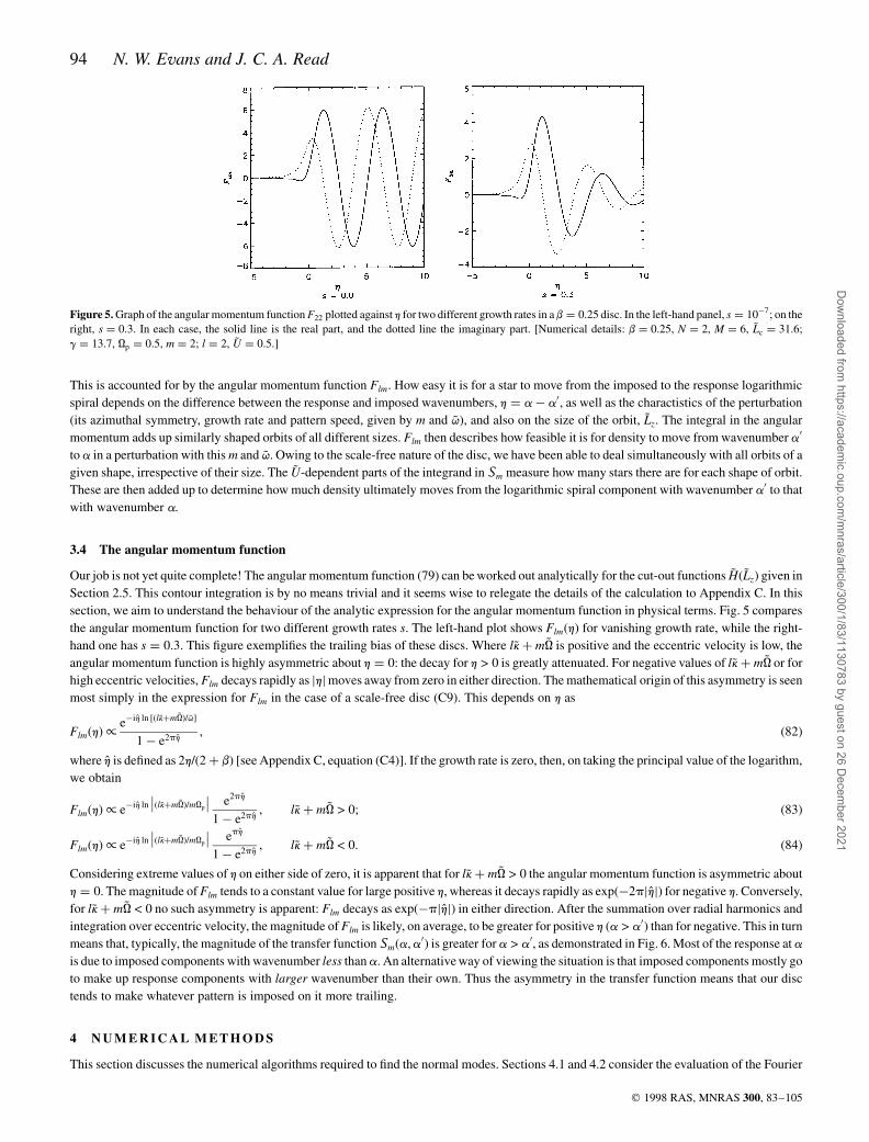
Our job is not yet quite complete! The angular momentum function (79) can be worked out analytically for the cut-out functions HðLzÞ given inSection 2.5. This contour integration is by no means trivial and it seems wise to relegate the details of the calculation to Appendix C. In thissection, we aim to understand the behaviour of the analytic expression for the angular momentum function in physical terms. Fig. 5 comparesthe angular momentum function for two different growth rates s. The left-hand plot shows FlmðhÞ for vanishing growth rate, while the right-hand one has s ¼ 0:3. This figure exemplifies the trailing bias of these discs. Where lk þ mQ is positive and the eccentric velocity is low, theangular momentum function is highly asymmetric about h ¼ 0: the decay for h > 0 is greatly attenuated. For negative values of lk þ mQ or forhigh eccentric velocities, Flm decays rapidly as jhj moves away from zero in either direction. The mathematical origin of this asymmetry is seenmost simply in the expression for Flm in the case of a scale-free disc (C9). This depends on h as

FlmðhÞ ∝ e¹ih ln ½ðlkþmQÞ=qÿ

1 ¹ e2ph; ð82Þ

where h is defined as 2h=ð2 þ bÞ [see Appendix C, equation (C4)]. If the growth rate is zero, then, on taking the principal value of the logarithm,we obtain

FlmðhÞ ∝ e¹ih ln��ðlkþmQÞ=mQp

�� e2ph

1 ¹ e2ph; lk þ mQ > 0; ð83Þ

FlmðhÞ ∝ e¹ih ln��ðlkþmQÞ=mQp

�� eph

1 ¹ e2ph; lk þ mQ < 0: ð84Þ

Considering extreme values of h on either side of zero, it is apparent that for lk þ mQ > 0 the angular momentum function is asymmetric abouth ¼ 0. The magnitude of Flm tends to a constant value for large positive h, whereas it decays rapidly as expð¹2pjhjÞ for negative h. Conversely,for lk þ mQ < 0 no such asymmetry is apparent: Flm decays as expð¹pjhjÞ in either direction. After the summation over radial harmonics andintegration over eccentric velocity, the magnitude of Flm is likely, on average, to be greater for positive h (a > a0) than for negative. This in turnmeans that, typically, the magnitude of the transfer function Smða;a0Þ is greater for a > a0, as demonstrated in Fig. 6. Most of the response at ais due to imposed components with wavenumber less than a. An alternative way of viewing the situation is that imposed components mostly goto make up response components with larger wavenumber than their own. Thus the asymmetry in the transfer function means that our disctends to make whatever pattern is imposed on it more trailing.

4 N U M E R I C A L M E T H O D S

This section discusses the numerical algorithms required to find the normal modes. Sections 4.1 and 4.2 consider the evaluation of the Fourier


q 1998 RAS, MNRAS 300, 83–105

Figure 5. Graph of the angular momentum function F22 plotted against h for two different growth rates in a b ¼ 0:25 disc. In the left-hand panel, s ¼ 10¹7; on theright, s ¼ 0:3. In each case, the solid line is the real part, and the dotted line the imaginary part. [Numerical details: b ¼ 0:25, N ¼ 2, M ¼ 6, Lc ¼ 31:6;g ¼ 13:7, Qp ¼ 0:5, m ¼ 2; l ¼ 2, U ¼ 0:5.]

Dow


ic.oup.com/m


ber 2021

coefficients and the transfer function respectively, whereas Section 4.3 presents the discretization of the integral equation. Again, let usemphasize that the numerical method is adopted – with a little streamlining – from Zang (1976).

4.1 The Fourier coefficient

The integrand in the definition of the Fourier coefficients (63) is periodic with period 2p in x. We are free to define x ¼ 0 to correspond topericentre. This means that at the time t ¼ 0, the star has radial coordinate R ¼ Rmin. As X is even, and Y is odd, about x ¼ 0, we can write

QlmðaÞ ¼1p

�p

0exp

ÿia ¹ 1

2

�X

� �cosðmY ¹ lxÞ dx: ð85Þ

The equations of motion (16) are solved by fourth-order Runge–Kutta integration (Press et al. 1989, ch. 15) to obtain the stellar position as afunction of time, and thus X and Y as a function of x. The integration over x is carried out by the midpoint method (Press et al. 1989, ch. 4),using nw points in the midpoint integration and 2nw in the Runge–Kutta. The problem is to choose nw large enough to obtain excellent accuracy,while keeping it as small as possible in order to save time. Eccentric orbits need more work to obtain good accuracy, so, as suggested by Zang(1976), nw is made to depend exponentially on U:

nw ¼ aacc expðbaccUÞ: ð86Þ

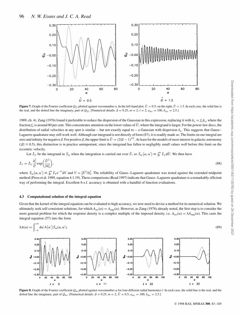
Values of aacc ¼ 10 and bacc ¼ 1:5 usually worked well. With these values, the Fourier coefficient is obtained with around 6 s.f. accuracy forlow-eccentricity orbits (U ¼ 0:5), but perhaps only 1 or 2 s.f. for high-eccentricity orbits (U ¼ 1:5). The Fourier coefficients are generallysmaller for higher values of the eccentric velocity. In the integrand for the transfer function, two Fourier coefficients are multiplied together atevery eccentric velocity. The accuracy with which the transfer function is obtained is thus dominated by the accuracy of the Fourier coefficientsat low eccentric velocities. This is useful, since the Fourier coefficients are costly to evaluate when the eccentric velocity is high. Fig. 7 showsthe Fourier coefficient as a function of wavenumber, for two different eccentric velocities. It is shown only for positive wavenumber. Itsbehaviour for negative wavenumber is readily deduced from the symmetry property QlmðaÞ ¼ Q¬

lmð¹aÞ. We see that U controls the amplitudeand the frequency of oscillation of Qlm. Fig. 8 compares Fourier coefficients at different radial harmonics. For high values of l, Qlm remainsclose to zero until a is large; thereafter it oscillates with lower frequency. Logarithmic spiral components must be tightly wound in order toexcite responses at high radial harmonics.

4.2 The transfer function

The expression for the transfer function (78) involves a sum over radial harmonic l from ¹∞ to þ∞. Fortunately, the magnitude of the terms inthis sum decreases sharply with jlj. Negative values of l decrease their contribution faster than positive l. A good approximation is given bysumming from l ¼ lmin to l ¼ lmax, where lmin is negative and jlminj is less than lmax. Values of lmin ¼ ¹20, lmax ¼ 30 usually worked well. Thetransfer function also contains an integral over eccentric velocity U, which adds up orbits of all possible shapes. The equivalent expression forthe Toomre–Zang disc (80) contains a Gaussian factor expð¹1

2U2=j2

uÞ. This prompted Zang (1976) to use Gauss–Laguerre quadrature toevaluate Sm. The fundamental formula is�∞

0f ðxÞe¹xdx <

XnGL

i¼1

wi f ðxiÞ; ð87Þ

where f ðxÞ is a smooth polynomial-like function. The weights wi and abscissae xi are well-known (see Abramowitz & Stegun 1965; Press et al.


q 1998 RAS, MNRAS 300, 83–105

Figure 6. Plot of the real part of the transfer function against a and a0. Notice the abrupt change on crossing the line a ¼ a0 – this is the trailing bias. [Numericaldetails: b ¼ 0:25, N ¼ 2, M ¼ 6, Lc ¼ 31:6; g ¼ 13:7, Qp ¼ 0:5, s ¼ 10¹7, m ¼ 2.]

Dow


ic.oup.com/m


ber 2021

1989, ch. 4). Zang (1976) found it preferable to reduce the dispersion of the Gaussian in this expression, replacing it with jn ¼ fjju, where thefraction fj is around 80 per cent. This concentrates attention on the lower values of U, where the integrand is larger. For the power-law discs, thedistribution of radial velocities at any spot is similar – but not exactly equal to – a Gaussian with dispersion ju. This suggests that Gauss–Laguerre quadrature may still work well. Although our integrand is not directly of form (87), it is readily made so. The limits on our integral arezero and infinity for negative b. For positive b, the upper limit is U ¼ ð2=b ¹ 1Þ1=2. At least for the models of most interest in galactic astronomy(jbj & 0:5), this distinction is in practice unimportant, since the integrand has fallen to negligibly small values well before this limit on theeccentric velocity.

Let IU be the integrand in Sm when the integration is carried out over U, so Sm a;a0ÿ �∝ �∞

0 IUdU. We then have

IV ¼ I Uj2

n

Uexp

U2

2j2n

� �; ð88Þ

where Sm a;a0ÿ �∝ �∞

0 IV e¹V dV and V ¼ 12U

2=j2

n. The reliability of Gauss–Laguerre quadrature was tested against the extended midpointmethod (Press et al. 1989, equation 4.1.19). These comparisons (Read 1997) indicate that Gauss–Laguerre quadrature is a remarkably efficientway of performing the integral. Excellent 6-s.f. accuracy is obtained with a handful of function evaluations.

4.3 Computational solution of the integral equation

Given that the kernel of the integral equation can be evaluated to high accuracy, we now need to devise a method for its numerical solution. Weultimately seek self-consistent solutions, for which AresðaÞ ¼ AimpðaÞ. However, as Zang (1976) already noted, the first step is to consider themore general problem for which the response density is a complex multiple of the imposed density, i.e. AresðaÞ ¼ lAimpðaÞ. This casts theintegral equation (57) into the form

lA að Þ ¼

�þ∞

¹∞da0A a0

ÿ �Smða;a0Þ; ð89Þ


q 1998 RAS, MNRAS 300, 83–105

Figure 7. Graph of the Fourier coefficient Q22 plotted against wavenumber a. In the left-hand plot, U ¼ 0:5; on the right, U ¼ 1:5. In each case, the solid line isthe real, and the dotted line the imaginary, part of Q22. [Numerical details: b ¼ 0:25, m ¼ 2, l ¼ 2; aacc ¼ 100, bacc ¼ 2:5.]

Figure 8. Graph of the Fourier coefficient Qlm plotted against wavenumber a for four different radial harmonics l. In each case, the solid line is the real, and thedotted line the imaginary, part of Qlm. [Numerical details: b ¼ 0:25, m ¼ 2, U ¼ 0:5; aacc ¼ 100, bacc ¼ 2:5.]

Dow


ic.oup.com/m


ber 2021

where we have dropped the subscripts on A. We refer to l as the mathematical eigenvalue. Of course, only the instance when l is unity carriesthe physical significance of a mode. The advantage of this mathematical artifice is that the integral equation (89) is in the standard form of ahomogeneous, linear, Fredholm equation of the second kind (see e.g. Courant & Hilbert 1953; Delves & Mohamed 1985). For a given value ofl, such an equation normally admits only the trivial solution, AðaÞ ; 0. The values of l for which non-trivial solutions exist are the eigenvaluesof the equation. We seek an iterative scheme which drives the eigenvalue to unity, thus providing a self-consistent mode. There is a closeanalogy between linear algebraic equations and linear integral equations. The former define relations between vectors in a finite-dimensionalvector space; the latter define relations between functions in an infinite-dimensional vector space (technically, a Banach space). This analogycan be made explicit by applying a quadrature rule to the integration in (89) to obtain

lA aj

ÿ �¼X

i

wiA ai

ÿ �Smðaj;aiÞ; ð90Þ

where wi are some appropriate weights. This general approach is called the Nystrom method (Delves & Mohamed 1985). It evidently reducesthe solution of an integral equation to the solution of an algebraic eigenvalue problem. The latter is a classic and well-studied area of numericalanalysis, for which many tried and tested techniques are available.

Much of the skill in the numerical solution of integral equations comes from the choice of quadrature rules and weights. Zang (1976)devised an elegant method based on locally approximating the kernel and the response by Lagrangian interpolating polynomials. This isnaturally adapted to the instance when the kernel varies on a much smaller scale than the solution. We follow this method, but we do not findZang’s splitting of the kernel of the integral equation into Hermitian and Volterra parts to be needed. First, to obtain smoother functions, theKalnajs gravity factor is extracted by defining

Sm a;a0ÿ �

¼ K a0;m

ÿ �Sm a;a0ÿ �

; A að Þ ¼AðaÞ

K a;mð Þ: ð91Þ

The eigenvalue equation now becomes

lA að Þ ¼ K a;mð Þ

�þ∞

¹∞da0A a0

ÿ �Sm a;a0ÿ �

: ð92Þ

Let us introduce a finite grid of points in wavenumber space, ar . If we need to know the value of A or Sm at a value of a intermediate betweenthe gridpoints ar and arþ1, we interpolate over the eight gridpoints from ar¹3 to arþ4. For eight equally spaced points Da apart, Lagrange’sclassic formula for the interpolating polynomial PðaÞ through N points f ðakÞ (Press et al. 1989, ch. 3) becomes

PðaÞ ¼Y8

i¼1

a ¹ arþi¹4

ÿ � X4

k¼¹3

ð¹1Þk

ð3 þ kÞ!ð4 ¹ kÞ!f ðarþkÞ

ðDaÞ7ða ¹ ar ¹ kDaÞ: ð93Þ

Defining x ¼ ða ¹ arÞ=Da, this becomes

PðaÞ ¼Y8

i¼1

x þ 4 ¹ ið ÞX4

k¼¹3

ð¹1Þk f ðarþkÞ

ð3 þ kÞ!ð4 ¹ kÞ!ðx ¹ kÞ¼X4

k¼¹3

Lk½xÿ f ðarþkÞ; ð94Þ

where

Lk½xÿ ¼ ð¹1Þk

Q8i¼1 x þ 4 ¹ ið Þ

ð3 þ kÞ!ð4 ¹ kÞ!ðx ¹ kÞ: ð95Þ

Then the interpolated approximations to the response and the transfer function are (cf. Zang 1976, appendix D)

Aða0Þ <X4

k¼¹3

Lk½x0ÿAðarþkÞ; Smða;a0Þ <

X4

k¼¹3

Lk½x0ÿSmða;arþkÞ; ð96Þ

where x0 ¼ ða0 ¹ arÞ=Da. The infinite range in the integral equation (89) is a kind of singularity. Truncation of the wavenumber range at largefinite values is the simplest but most brutal way of handling the singularity. In practice, we found this to be surprisingly effective. Wavenumberspace is approximated by a finite grid with n points along each side. We choose n, and the gridpoint spacing Da, so as to obtain a sufficientlyaccurate solution of the integral equation (57). The finite size of the grid means that we encounter problems when evaluating Aimp and Sm forvalues of a near the edges of the grid. We are interpolating over eight points, so we need data from a¹2 to anþ3. We deal with this problem bysimply assuming that our function is zero outside the grid. This is acceptable provided that the grid is large enough. Then the values of thekernel at the missing interpolation points are negligibly small. This procedure is justified empirically by the demonstration that themathematical eigenvalue converges to a value independent of grid size (Read 1997).

Substituting the Lagrange-interpolated approximations for Aimp and Sm (96) into the modified integral equation (92) , we obtain

lA að Þ ¼ K a;mð ÞX4

i¼¹3

X4

k¼¹3

�an

a1

da0Lia0 ¹ ar

Da

� �Lk

a0 ¹ ar

Da

� �Aða0

rþiÞSmða;a0rþkÞ: ð97Þ


q 1998 RAS, MNRAS 300, 83–105

Dow


ic.oup.com/m


ber 2021

Of course, the integration over wavenumber now runs from a ¼ a1 to an, instead of from a ¼ ¹∞ to ∞. We break this integration into nportions of Da:

lA að Þ ¼ K a;mð ÞXn

r¼1

X4

i¼¹3

X4

k¼¹3

�arþDa

ar

da0Lia0 ¹ ar

Da

� �Lk

a0 ¹ ar

Da

� �Aða0

rþiÞSmða;a0rþkÞ: ð98Þ

Then, changing variables to x0 ¼ ða0 ¹ arÞ=Da, we obtain

lA að Þ ¼ K a;mð ÞXn

r¼1

X4

i¼¹3

X4

k¼¹3

AðarþiÞSmða;arþkÞDa

�1

0dx0Li½x

0ÿLk½x0ÿ: ð99Þ

Let us define the weighting coefficients Cik by (cf. Zang 1976, appendix D)

Cik ¼ Da

�1

0dxLi½xÿLk½xÿ: ð100Þ

Although there appear to be 64 Cik , only 20 of them are independent, because of the symmetry properties Cik ; Cki, and Cik ; Cð1¹iÞð1¹kÞ. Theweighting coefficients are easily evaluated using the midpoint method given in Press et al. (1989, ch. 4). They are tabulated in Read (1997).Equation (97) can now be written as

lA aj

ÿ �¼ K aj;m

ÿ �Xn

r¼1

X4

i¼¹3

X4

k¼¹3

CikSmðaj;arþkÞAðarþiÞ: ð101Þ

Terms in this multiple sum for which r þ i is less than 1 or greater than n contribute nothing. We can thus write the above equation in terms of asingle sum from a1 to an, and collect the weighting coefficients Cik , smoothed transfer function Sm and density profile A together into a singlequantity S:

lAðajÞ ¼Xn

s¼1

SjsAðasÞ: ð102Þ

This is of course just a matrix equation for the mathematical eigenvalue l. If there is an eigenvalue of the matrix S equal to unity, then thecorresponding eigenvector A gives us a self-consistent mode, i.e. a self-sustaining density perturbation. Sjs cannot be simply expressed in termsof Cik , Sm and A, but we see that it represents the total coefficient of AðasÞ in equation (101).

Having obtained the matrix Sjs, it is reasonably straightforward to find its eigenvalues using the eigensystem package (eispack) developedby Smith et al. (1972). This returns the eigenvalues of a matrix and, optionally, the corresponding eigenvectors. The power method can also beused to provide an independent check on the largest eigenvalue. This relies on repeated application of the matrix S to a test vector t (Ralston &Rabinowitz 1978, ch. 8, section 7). Probably the most important factors in achieving excellent accuracy in the eigenvalues are the size andfineness of the grid. The range of the grid, ðn ¹ 1ÞDa, typically needs to be around 50 in order for the mathematical eigenvalue to be accurate to6 s.f. A grid spacing of Da ¼ 0:2 is usually sufficient. However, suitable values necessarily depend to some extent on the form of the mode. Forinstance, for high azimuthal harmonics, the modes tend to be tightly wrapped, requiring a more extensive grid.

Having established that the mathematical eigenvalue can be found to good accuracy, let us consider how to locate the unit eigenvalueswhich correspond to self-consistent modes. We are investigating modes of a given azimuthal symmetry in a disc with given density profile.This means that m, b, N, M and Lc are held fixed. It leaves us free to adjust g, s and Qp. A disc at a given temperature, if it admits a mode at all,generally does so only for a particular growth rate and pattern speed. We therefore hold g fixed, and adjust s and Qp until a mode is found. This isin fact a search for the root of the equation l ¼ 1 in only one dimension, since the mathematical eigenvalue l is an analytic function of thecomplex frequency q ¼ mQp þ is. The Newton–Raphson method is extremely effective at locating such roots. When the disc is sufficientlyhot, it is generally completely stable. As the disc is cooled, instabilities set in through the marginal modes, for which the growth rate s is zero.We are therefore often interested in the marginally stable modes. To find these, s is set to some vanishingly small value, and a two-dimensionalsearch is performed for the critical pattern speed Qp and temperature g using the Newton–Raphson method in two dimensions.

4.4 The special case of axisymmetry

In the case of an axisymmetric perturbation, the integral equation admits certain symmetries. The first simplification is that the frequency ispurely imaginary: q ¼ is. Secondly, the integral equation is equivalent to one with a Hermitian kernel, and hence must have purely realeigenvalues. It is straightforward to deduce the symmetries

Fl0ðhÞ ¼ F¬¹l0ð¹hÞ; Q¬

l0ðaÞ ¼ Ql0ð¹aÞ; Q¹l0ðaÞ ¼ Ql0ðaÞ: ð103Þ

Let us now recast the integral equation (89) into a form with a Hermitian kernel by defining a modified transfer function and density transform(Zang 1976)

T0ða;a0Þ ¼

��Kða; 0Þ

Kða0; 0Þ

rS0ða;a

0Þ; BðaÞ ¼��Kða; 0Þ

pAðaÞ: ð104Þ


q 1998 RAS, MNRAS 300, 83–105

Dow


ic.oup.com/m


ber 2021

The integral equation (89) now becomes

lBðaÞ ¼

�þ∞

¹∞da0Bða0ÞT0ða;a

0Þ: ð105Þ

The value of this transformation is that T0ða;a0Þ is Hermitian, namely

T ¬0 ða0

;aÞ ¼ T0ða;a0Þ: ð106Þ

The modified integral equation (105) is thus a homogeneous, linear Fredholm integral equation with a Hermitian kernel. It must therefore havereal eigenvalues and orthogonal eigenfunctions (Tricomi 1985). This occurs because the mathematical eigenvalues have no dependence onpattern speed. In general, the mathematical eigenvalue l is an analytic function of the complex frequency q. Only for m ¼ 0 is the frequencypurely imaginary and the problem one-dimensional.

There is a further symmetry. We make the transformations a → ¹a, a0 → ¹a0, l → ¹l, so as to obtain T¬0 ð¹a;¹a0Þ. Using the symmetry

properties of the Fourier coefficients and the angular momentum function (103) along with that of the Kalnajs gravity factor, we obtain theresult

T ¬0 ð¹a;¹a0Þ ¼ T0ða;a

0Þ: ð107Þ

This has the consequence that the eigenvalues are degenerate. If BðaÞ is an eigenvector with eigenvalue l, then so is B¬ð¹aÞ. To see this, wemake the transformations a → ¹a, a0 → ¹a0 in the modified integral equation (105), and take the complex conjugate. We obtain

lB¬ð¹aÞ ¼ ¹

�¹∞

∞da0B¬ð¹a0ÞT¬

0 ð¹a;¹a0Þ ¼

�þ∞

¹∞da0B¬ð¹a0ÞT0ða;a

0Þ: ð108Þ

In other words, B¬ð¹aÞ also satisfies the integral equation (105). In terms of our original density transforms, AðaÞ and A¬ð¹aÞ are a degeneratepair with the same eigenvalue l. This is just the anti-spiral theorem (Lynden-Bell & Ostriker 1967; Kalnajs 1971) for axisymmetricperturbations.

5 C O N C L U S I O N S

This paper has set up the machinery for an investigation into the large-scale, global, modes of the power-law discs. The Fredholm integralequation for the normal modes has been derived. This is done by linearizing the collisionless Boltzmann equation to find the response densitycorresponding to any imposed density and potential. The normal modes are given by equating the imposed density to the response density. Thisscheme is implemented in Fourier space, so that the Fredholm integral equation relates the transform of the imposed density to the transform ofthe response density. Numerical strategies are given to discretize the integral equation to yield a matrix equation. This requires some care as thekernel of the integral equation is either singular (as in the case of the self-consistent disc) or almost so (the cut-out discs). The problem oflocating the normal modes is thus reduced to an algebraic eigenvalue problem, for which a wealth of standard techniques are available. Thecrucial simplification underlying the analysis is that the force law describing the gravity field of the galactic disc is scale-free. It is this thatensures that orbits passing through any one spot in the disc are simply scaled copies of the orbits passing through any other spot. When theorbits are forced by a scale-free logarithmic spiral perturbation, the response of all orbits of the same eccentricity can be computed at the sametime. It only remains to add up the contributions at every eccentricity. For a disc with an arbitrary force law, such simplification is not possible.

Let us again emphasize that nearly all the computational techniques required to study the stability of the power-law discs were developedby Zang (1976) in his pioneering study of the disc with a completely flat rotation curve. Our contribution consists only of deriving theextensions to study the complete family of scale-free power-law discs. This paper has discussed just the algorithms – the aim has been topresent all the mathematical and computational details for reference here. The following paper in this issue of Monthly Notices implements themachinery discussed here to provide a complete description of the spiral modes of the self-consistent and cut-out power-law discs. A fastcomputer code is developed which gives the growth rates and pattern speeds of the normal modes for any power-law disc in a matter of minuteswhen run on a modern workstation.

AC K N OW L E D G M E N T S

NWE thanks Alar Toomre for much generous and helpful advice on how to extend the analysis in Zang’s thesis to the family of power-lawdiscs. NWE is also grateful to the trustees of the Lindemann Fellowship for an award which enabled him to spend the year of 1994 at theMassachusetts Institute of Technology. He is supported by the Royal Society. JCAR thanks the Particle Physics and Astronomy ResearchCouncil for a research studentship.

REFERENCES

Abramowitz M., Stegun I. A., 1965, Handbook of Mathematical Functions. Dover, New YorkBinney J., Tremaine S., 1987, Galactic Dynamics. Princeton Univ. Press, Princeton, NJBisnovatyi-Kogan E., 1976, Sov. Astron. Lett., 1, 177Casertano S., van Gorkom J. H., 1991, AJ, 101, 1231Courant R., Hilbert D., 1953, Methods of Mathematical Physics. Interscience, New York


q 1998 RAS, MNRAS 300, 83–105

Dow


ic.oup.com/m


ber 2021

Delves L. M., Mohamed J. L., 1985, Computational Methods for Integral Equations. Cambridge Univ. Press, CambridgeEarn D. J. D., 1993, PhD thesis, Cambridge UniversityEarn D. J. D., Sellwood J. A., 1995, ApJ, 451, 533Evans N. W., 1994, MNRAS, 267, 333Evans N. W., Collett J. L., 1993, MNRAS, 264, 353Jeans J. H., 1919, Problems of Cosmogony & Stellar Dynamics. Cambridge Univ. Press, CambridgeKalnajs A. J., 1965, PhD thesis, Harvard UniversityKalnajs A. J., 1971, ApJ, 166, 275Kalnajs A. J., 1972, ApJ, 175, 63Lemos J. P. S., Kalnajs A. J., Lynden-Bell D., 1991, ApJ, 375, 484Lynden-Bell D., Ostriker J. P., 1967, MNRAS, 136, 101Merritt D., Sellwood J. A., 1994, ApJ, 425, 551Mestel L., 1963, MNRAS, 126, 553Mihalas D., Binney J. J., 1987, Galactic Astronomy. W. H. Freeman, San FranciscoOstriker J. P., Peebles P. J. E., 1973, ApJ, 186, 467Palmer P. L., Papaloizou J., 1990, MNRAS, 243, 263Press W., Flannery B., Teukolsky S., Vetterling W., 1989, Numerical recipes: the art of scientific computing. Cambridge Univ. Press, CambridgePrudnikov A. P., Brychkov Y. A., Mavichev O., 1986, Integrals and Series, Vol. 1. Gordon and Breach, New YorkRalston A., Rabinowitz P., 1978, A First Course in Numerical Analysis. McGraw-Hill, New YorkRead J. C. A., 1997, PhD thesis, Oxford UniversityRubin V. C., Ford W. K., Thonnard N., 1978, ApJ, 225, L107Schmitz F., Ebert R., 1987, A&A, 181, 41Sellwood J. A., Athanassoula E., 1986, MNRAS, 221, 195Smith B. T., Boyle J. M., Dongarra J. J., Garbow B. S., Ikebe Y., Klema V. C., Moler C. B., 1972, Lecture Notes in Computer Science, Vol. 6, 2nd edn. Springer-

Verlag, BerlinSnow C., 1952, Hypergeometric and Legendre Functions with Applications to the Integral Equations of Potential Theory. National Bureau of Standards,

WashingtonToomre A., 1977, ARA&A, 15, 437Toomre A., 1981, in Fall S. M., Lynden-Bell D., eds, The Structure and Evolution of Normal Galaxies. Cambridge Univ. Press, Cambridge, p. 111Tricomi F., 1985, Integral Equations. Dover, New YorkZang T. A., 1976, PhD thesis, Massachusetts Institute of Technology

A P P E N D I X A : S I N G L E - E C C E N T R I C I T Y D I S T R I B U T I O N F U N C T I O N S

In the main body of the paper, we have used stellar distribution functions for the power-law discs that are built from powers of energy andangular momentum. Many other equilibrium distribution functions are possible. In this Appendix, we consider discs in which all the stars havethe same shape of orbit, characterized by an eccentric velocity U ¼ Ur. Mathematically, we look for distribution functions of the form

fs ¼ FðRHÞdðU ¹ UrÞ: ðA1Þ

The surface density is

Seq ¼ S0R0

R

� �1þb

¼

� �fsðu; vÞdu dv: ðA2Þ

We transform this to an integral over U and RH, using the Jacobian

du dv ¼ dU dRH 1 ¹b

2

� �vb

RR0

RH

� �b=2 U��U2 þ 1 ¹ R¹2 þ 2

bðR¹b ¹ 1Þ

q ; ðA3Þ

and substitute our assumed distribution function

S0R0

R

� �1þb

¼ 1 ¹b

2

� �vb

R

ZZR0

RH

� �b=2 U FðRHÞ dðU ¹ UrÞ dU dRH��U2 þ 1 ¹ R¹2 þ 2

bðRb ¹ 1Þ

q : ðA4Þ

We integrate over U, and then transform the integral over RH to one over R ¼ R=RH:

S0R0

R

� �1þb=2

¼ 1 ¹b

2

� �2vbUr

�Rmax

Rmin

Rb=2F R=Rÿ �

dR

R2��U2

r þ 1 ¹ R¹2 þ 2bðRb ¹ 1Þ

q ; ðA5Þ

where Ur is the value of Ur in dimensionless units. Looking at the powers of R, we can guess at a solution of this integral equation, namelyFðR=RÞ ¼ kðR=RÞ1þb=2

: Substituting this into (A5), and remembering the definition of the auxiliary integral J nðUÞ (18), we can solve for k andobtain

k ¼S0R1þb=2

0

ð1 ¹ b2ÞvbUrJ 1¹bðUrÞ

¼S0R1þb

0

1 ¹ b2

ÿ �Rb=2

H UrJ 1¹bðUrÞ: ðA6Þ


q 1998 RAS, MNRAS 300, 83–105

Dow


ic.oup.com/m


ber 2021

The distribution function is then

fsðU;RHÞ ¼S0R1þb

0

1 ¹ b2

ÿ �UrJ 1¹bðUrÞ

dðU ¹ UrÞ

R1þbH

: ðA7Þ

This expression is valid for b ¼ 0, in which case the appropriate form for the auxiliary integral J 1 (19) must be used.All the stars in this disc have orbits of the same shape, but different size. Each star sweeps out an annulus as it orbits. The relative width of

this annulus depends on the eccentric velocity Ur, but the overall size of the annulus depends on RH. It is easy to imagine that if we add up annuliwith a variety of RH in suitable proportions, we could recover the surface density of the equilibrium disc; and this is what the distributionfunction (A7) does. It seems intuitively right that the number of annuli needed falls off with RH at the same rate as the surface density falls offwith R. Similarly, we can see why the total number of annuli depends inversely on eccentric velocity Ur: for high Ur , the annuli are very wide,and few are needed; for low Ur, the converse is true.

A P P E N D I X B : R E F E R E N C E TA B L E O F D I M E N S I O N L E S S Q UA N T I T I E S

Quantity For the Toomre–Zang disc For the general power-law disc

RH Home radius RH ¼ RH=R0 RH ¼ RH=R0

t Time t ¼ v0RH

t t ¼vb

RHR¹b=2

H t

u Radial velocity u ¼ dRdt ¼ u

v0u ¼ dR

dt ¼ uvb

Rb=2H

v Tangential velocity v ¼ Rdvdt ¼ v

v0v ¼ R¹1 v ¼ Rdv

dt ¼ vvb

Rb=2H v ¼ R¹1

E Energy E ¼ Ev2

0; E ¼ 1

2 u2 þ v2ÿ �¹ ln R0

R E ¼ Ev2

b

RbH ; E ¼ 1

2 u2 þ v2ÿ �¹ 1

bRb

Lz Angular momentum Lz ¼Lz

R0v0¼ R Lz ¼

LzR0vb

¼ R1¹b=2

U Eccentric velocity U ¼ Uv0

U ¼ Uvb

Rb=2H

U2 ¼ u2 ¹ 1 þ R¹2 þ 2 ln R U2 ¼ u2 ¹ 1 þ R¹2 ¹ 2b

R¹b ¹ 1� �

J n Auxiliary integral J n ¼� Rmax

Rmin

2dRRn U2þ1¹R¹2¹2 ln Rð Þ1=2 J n ¼

� Rmax

Rmin

2dR

Rn U2þ1¹R¹2þ2b

R¹b¹1ð Þ� �1=2

k Radial frequency k ¼ RHv0

k ¼ 2pJ 0

k ¼ RHvb

Rb=2H k ¼ 2p

J 0

Q Angular frequency Q ¼ RHv0

Q ¼ J 2J 0

Q ¼ RHvb

Rb=2H Q ¼ J 2

J 0

k0 Epicyclic frequency k0 ¼��2

pk0 ¼

��2 ¹ b

pQ0 Circular frequency Q0 ¼ 1 Q0 ¼ 1

x Orbital phase x ¼ kt ¼ kt x ¼ kt ¼ kt

Y Angular deviation Y ¼ v ¹ Q t ¼ v ¹ Q t Y ¼ v ¹ Qt ¼ v ¹ Qt

x Logarithmic radius x ¼ ln RR0

� �x ¼ ln R

R0

� �X Scaled logarithmic radius X ¼ ln R

RH

� �¼ ln R X ¼ ln R

RH

� �¼ ln R

ju Radial velocity dispersion j2u ¼ 1

1þgj2

u ¼ 11þgþ2b

g Anisotropy parameter g ¼ 1j2

u¹ 1 g ¼ 1

j2u¹ 1 ¹ 2b


q 1998 RAS, MNRAS 300, 83–105

Dow


ic.oup.com/m


ber 2021

A P P E N D I X C : T H E A N G U L A R M O M E N T U M F U N C T I O N

In this appendix, we derive the forms of the angular momentum function by explicitly performing the contour integration over angularmomentum Lz. Let us recall that the angular momentum function is

Flm ¼1

2p

�∞

0

e¹ih½2=ð2¹bÞÿ ln Lz



bU2 þ b ¹ 2

�� ¹ gm

� �H ¹ mLz

dH

dLz

� �dLz

Lz:

The integration is carried out over the variable h defined by

h ¼2 þ b

2 ¹ bln Lz; HðLzÞ ¼ H ðhÞ: ðC1Þ

It is performed for three different cut-out factors, namely the self-consistent disc, the inner cut-out disc and the doubly cut-out disc (all definedin equation 41). We proceed by splitting up the integral into two parts:

FlmðhÞ ¼ ðlk þ mQÞ2 þ 2g ¹ bg

bU2 þ b ¹ 2

�� ¹ gm

� �J1 ¹ mJ2; ðC2Þ

where

J1ðb; h; LcÞ ¼1

2p

2 ¹ b

2 þ b

�∞

¹∞

e¹ih½2=ð2þbÞÿh

lk þ mQ ¹ qehH ðhÞdh; J2ðb; h; LcÞ ¼

12p

�∞

¹∞

e¹ih½2=ð2þbÞÿh

lk þ mQ ¹ qeh

dHdh

dh: ðC3Þ

We need evaluate these only for the case b ¼ 0, since the general integrals are related to the b ¼ 0 integrals as

J1ðb; h; LcÞ ¼2 ¹ b

2 þ bJ1 0; h; Lð2þbÞ=ð2¹bÞ

c

� �; J2ðb; h; LcÞ ¼ J2 0; h; Lð2þbÞ=ð2¹bÞ

c

� �; with h ; h ×

22 þ b

: ðC4Þ

Lc has been included as an argument, although clearly this is only relevant to the doubly cut-out disc. We suppress the third argument unlessneeded.

C1 The self-consistent disc

Here

J1ð0; hÞ ¼1

2p

�∞

¹∞

e¹ihh

lk þ mQ ¹ qehdh; J2ð0; hÞ ¼ 0: ðC5Þ

We first consider the case q Þ 0. J1 may be evaluated by contour integration. The integrand has poles when hn ¼ ln½ðlk þ mQÞ=qÿ þ 2nip,where n is an integer. The poles occur at intervals along a line parallel to the imaginary axis. Note that q is not in general real (q ¼ mQp þ is),so that the poles are displaced from the lines h ¼ 2nip. We evaluate the integral

12p

�elhe¹ihh

lk þ mQ ¹ qehdh; ðC6Þ

around a rectangular contour as shown in the left-hand plot of Fig. C1, with long sides at h ¼ 0, h ¼ 2ip, and short edges at 6L, enclosing thepole at h ¼ ln½ðlk þ mQÞ=qÿ. Here the logarithm denotes the principal value, i.e. the imaginary part lies between 0 and 2p. Then

12p

�L

¹L

elhe¹ihhdh

lk þ mQ ¹ qeh¹

e2iple2ph

2p

�L

¹L

elhe¹ihhdh

lk þ mQ ¹ qehþ

12p

�2p

0

elLeyheilye¹ihLdh

lk þ mQ ¹ qeiyeL

¹1

2p

�2p

0

e¹lLeyheilyeihLdh

lk þ mQ ¹ qeiye¹L¼ ¹

i

lk þ mQel ln½ðlkþmQÞ=qÿe¹h ln½ðlkþmQÞ=qÿ

: ðC7Þ


q 1998 RAS, MNRAS 300, 83–105

Figure C1. Contours and poles for the self-consistent disc. The left-hand plot shows the contour used for h Þ 0, and the right-hand plot that for h ¼ 0.

Dow


ic.oup.com/m


ber 2021

Taking L → ∞, and then l → 0, we obtain the result

J1ð0; hÞ ¼ ¹ie¹ih ln½ðlkþmQÞ=qÿ

ðlk þ mQÞ 1 ¹ e2phÿ � : ðC8Þ

Generalizing this result to all b as described above, we obtain

FlmðhÞ ¼ ¹2 ¹ b

2 þ b

2 þ 2g ¹ bg

bU2 þ b ¹ 2

�� ¹ gm

lk þ mQ

� �ie¹ih ln ½ðlkþmQÞ=qÿ

1 ¹ e2phÿ � ; h Þ 0: ðC9Þ

This expression is singular when h ¼ 0. As we now demonstrate, FlmðhÞ contains a delta-function at h ¼ 0. For the case Qp ¼ 0, s ¼ 0, we canintegrate the expression for FlmðhÞ directly:

J1ð0; hÞ ¼1

lk þ mQ

12p

�∞

¹∞e¹ihhdh ¼

1

lk þ mQdðhÞ; ðC10Þ

and so for the general power-law disc

FlmðhÞ ¼2 ¹ b

2 þ b

2 þ 2g ¹ bg

bU2 þ b ¹ 2

�� ¹ gm

lk þ mQ

� �dðhÞ: ðC11Þ

To obtain the expression for general Qp and s, we write

J1ð0; hÞ ¼ Jð1Þ1 ð0; hÞ þ Jð2Þ

1 dðhÞ; ðC12Þ

where Jð1Þ1 ð0; hÞ is equal to our previous expression (C8) for J1ð0; hÞ. We integrate (C12) over h, thus smoothing out the delta-function:�þe

h¼¹edh J1ð0; hÞ ¼

�þe

h¼¹edh Jð1Þ

1 ð0; hÞ þ Jð2Þ1

�þe

h¼¹edh dðhÞ: ðC13Þ

We now let e → 0. We see from the expression for Jð1Þ1 ðhÞ already obtained (C8) that Jð1Þ

1 ðhÞ is odd in the limit of vanishingly small h. It thereforecontributes nothing in (C13). Using the expression (C3) for J1ð0; hÞ, we obtain

Jð2Þ1 ¼ lim

e→0

12p

�þe

h¼¹edh

�∞

h¼¹∞dh

e¹ihh

lk þ mQ ¹ qeh: ðC14Þ

Swapping the order of integration and performing the integration over h, we obtain

Jð2Þ1 ¼ lim

e→0

12pi

�∞

h¼¹∞

dhh

eieh ¹ e¹ieh

lk þ mQ ¹ qeh: ðC15Þ

We evaluate this by carrying out two separate contour integrals. For the integral with e¹ieh, we close the contour in the lower half-plane, asshown in the right-hand plot of Fig. C1. As usual, we take the radius of the inner semi-circle to zero, and that of the outer semi-circle to infinity.The integrand then vanishes on the outer semi-circle, and we obtain

12pi

�∞

h¼¹∞

dhh

e¹ieh

lk þ mQ ¹ qeh¼

1

lk þ mQ

X¹∞

n¼¹1

e¹ie ln ½ðlkþmQÞ=qÿe2npe

ln ½ðlk þ mQÞ=qÿ þ 2inp¹

12

1

lk þ mQ ¹ q: ðC16Þ

The integral with eþieh is evaluated over an analogous contour in the upper half-plane. We obtain

12pi

�∞

h¼¹∞

dhh

eieh

lk þ mQ ¹ qeh¼ ¹

1

lk þ mQ

X∞

n¼0

eie ln½ðlkþmQÞ=qÿe¹2npe

ln½ðlk þ mQÞ=qÿ þ 2inpþ

12

1

lk þ mQ ¹ q: ðC17Þ

Subtracting these two results and taking the limit e → 0, we obtain

12pi

�∞

h¼¹∞

dhh

eieh ¹ e¹ieh

lk þ mQ ¹ qeh¼

1

lk þ mQ ¹ qþ

i

lk þ mQ

X∞

n¼¹∞

1

2np ¹ i ln½ðlk þ mQÞ=qÿ: ðC18Þ

The sum can be explicitly evaluated:X∞

n¼¹∞

12np ¹ iz

¼ ¹1iz

þX¹∞

n¼¹1

12np ¹ iz

þX∞

n¼1

12np ¹ iz

¼izþ 2iz

X∞

n¼1

1ð2npÞ2 þ z2

¼iz

4p2

X∞

n¼¹∞

1ðn þ iz=2pÞðn ¹ iz=2pÞ

¼ ¹12

cotiz2

¼ ¹i2

e¹z þ 1e¹z ¹ 1

; ðC19Þ

where we have used the standard result (Prudnikov, Brychkov & Mavichev 1986, equation 5.1.6.4)X∞

n¼¹∞

1ðn þ aÞðn þ bÞ

¼p

b ¹ aðcot pa ¹ cot pbÞ: ðC20Þ


q 1998 RAS, MNRAS 300, 83–105

Dow


ic.oup.com/m


ber 2021

Thus we obtain

Jð2Þ1 ¼

1

2ðlk þ mQÞ: ðC21Þ

The angular momentum function for the self-consistent disc is then

FlmðhÞ ¼2 ¹ b

2 þ b

2 þ 2g ¹ bg

bU2 þ b ¹ 2

�� ¹ gm

lk þ mQ

� �12dðhÞ ¹

ie¹ih ln ½ðlkþmQÞ=qÿ

1 ¹ e2ph

" #: ðC22Þ

The corresponding result for the Toomre–Zang disc is [correcting a typographical error in Zang (1976), equation (Z3.43)]

FlmðhÞ ¼ g þ 1 ¹gm

lk þ mQ

� �12

dðhÞ ¹ie¹ih ln ½ðlkþmQÞ=qÿ

1 ¹ e2ph

" #: ðC23Þ

C2 The inner cut-out disc

Here, we must evaluate

J1ð0; hÞ ¼1

2p

�∞

¹∞

e¹ihh

lk þ mQ ¹ qeh

eNh

eNh þ 1dh; J2ð0; hÞ ¼

12p

�∞

¹∞

e¹ihh

lk þ mQ ¹ qeh

NeNh

eNh þ 1ÿ �2 dh: ðC24Þ

Again the integrands have poles when h ¼ ln½ðlk þ mQÞ=qÿ þ 2nip. However, they now also have poles along the imaginary axis, athj ¼ ð2j ¹ 1Þip=N, where j is an integer. We integrate around the same rectangular contour as for the self-consistent disc (Fig. C1). As well asthe pole at ln½ðlk þ mQÞ=qÿ, we now also enclose N poles lying on the imaginary axis. Adding up the residues from all these poles, we obtain theresult

J1ð0; hÞ ¼¹i

1 ¹ e2ph

ðlk þ mQÞN¹1e¹ih ln ½ðlkþmQÞ=qÿ

ðlk þ mQÞN þ qN¹

1N

XN

j¼1

e½ð2j¹1Þ=Nÿph

lk þ mQ ¹ qe½ð2j¹1Þ=Nÿip

" #; ðC25Þ

J2ð0; hÞ ¼ ¹i

1 ¹ e2ph×

ðlk þ mQÞN¹1NqNe¹ih ln ½ðlkþmQÞ=qÿ

ðlk þ mQÞN þ qN� �2 þ

1N

XN

j¼1

e½ð2j¹1Þ=Nÿph

lk þ mQ ¹ qe½ð2j¹1Þ=Nÿipih ¹

qe½ð2j¹1Þ=Nÿip


" #( ): ðC26Þ

For b Þ 0, we obtain the angular momentum function

Flmðh Þ 0Þ ¼ ¹i

1 ¹ e2ph×

ðlk þ mQÞN¹1e¹ih ln ½ðlkþmQÞ=qÿ

ðlk þ mQÞN þ qN

��"

2 ¹ b

2 þ bðlk þ mQÞ

2 þ 2g ¹ bg

bU2 þ b ¹ 2

�� ¹ gm

� �¹

mNqN

ðlk þ mQÞN þ qN

� �

¹1N

XN

j¼1

e½ð2j¹1Þ=Nÿph


mqe½ð2j¹1Þ=Nÿip

lk þ mQ ¹ qe½ð2j¹1Þ=Nÿip¹ imh þ

2 ¹ b

2 þ bðlk þ mQÞ

2 þ 2g ¹ bg

bU2 þ b ¹ 2

�� ¹ gm

� �( )��#: ðC27Þ

We can use l’Hopital’s rule to obtain the result for h ¼ 0. This requires that both the numerator and denominator of (C27) are zero in the limith → 0. The denominator ð1 ¹ e2phÞ is obviously zero in this limit, and it can be shown that the numerator is also (e.g. it is readily apparent forN ¼ 1). Application of l’Hopital’s rule then yields

Flmðh ¼ 0Þ ¼ ¹i

2p

iðlk þ mQÞN¹1 ln lkþmQq

ðlk þ mQÞN þ qN

2 ¹ b

2 þ bðlk þ mQÞ

2 þ 2g ¹ bg

bU2 þ b ¹ 2

�� ¹ gm

� �¹

mNqN

ðlk þ mQÞN þ qN

� ��"

þ1N

XN

j¼1

1


×

ð2j ¹ 1Þ

p

Nmqe½ð2j¹1Þ=Nÿip

lk þ mQ ¹ qe½ð2j¹1Þ=Nÿipþ

2 ¹ b

2 þ bðlk þ mQÞ

2 þ 2g ¹ bg

bU2 þ b ¹ 2

�� ¹ gm

� �( )¹ im

!��#: ðC28Þ

C3 The doubly cut-out disc

We briefly summarize the results for the doubly cut-out discs. Here,

J1ð0; h; LcÞ ¼1

2p

�∞

¹∞

e¹ihh

lk þ mQ ¹ qeh

eNh

ðeNh þ 1ÞðL¹Mbc eMh þ 1Þ

dh; ðC29Þ

J2ð0; h; LcÞ ¼1

2p

�∞

¹∞

e¹ihh

lk þ mQ ¹ qeh

NeNh L¹Mbc eMh þ 1

� �¹ ML

¹Mbc eNheMh

ðeNh þ 1Þ2ðL¹Mbc eMh þ 1Þ2

dh: ðC30Þ

The integrand now has additional poles at hk ¼ ð2k ¹ 1Þip=M þ ð2 þ bÞ=ð2 ¹ bÞ × ln Lc, where k is an integer. We thus obtain a second sum,


q 1998 RAS, MNRAS 300, 83–105

Dow


ic.oup.com/m


ber 2021

and Flm becomes

Flmðh Þ 0Þ ¼¹i

1 ¹ e2ph×

"�� ðlk þ mQÞN¹1LMbc qMe¹ih ln ½ðlkþmQÞ=qÿ

½ðlk þ mQÞN þ qNÿ½ðlk þ mQÞM þ LMbc qMÿ

×2 ¹ b

2 þ bðlk þ mQÞ

2 þ 2g ¹ bg

bU2 þ b ¹ 2

�� ¹ gm

� �¹

mNqN

ðlk þ mQÞN þ qNþ

mMðlk þ mQÞM

ðlk þ mQÞM þ LMbc qM

( )

¹L

Mbc

N

XN

j¼1

e½ð2j¹1Þ=Nÿph

½eð2j¹1ÞMN ip þ L

Mbc ÿ½lk þ mQ ¹ qe½ð2j¹1Þ=Nÿipÿ

mqe½ð2j¹1Þ=Nÿip

lk þ mQ ¹ qe½ð2j¹1Þ=Nÿip¹ imh þ

2 ¹ b

2 þ bðlk þ mQÞ

2 þ 2g ¹ bg

bU2 þ b ¹ 2

�� ¹ gm

� �( )

þL

Nbc

Me¹ih½ð2þbÞ=ð2¹bÞÿ ln Lc

XMk¼1

e½ð2k¹1Þ=Mÿph

½e¹ð2k¹1ÞNMip þ L

Nbc ÿ½lk þ mQ ¹ qLð2þbÞ=ð2¹bÞ

c e½ð2k¹1Þ=Mÿipÿ

×mqLð2þbÞ=ð2¹bÞ

c e½ð2k¹1Þ=Mÿip

lk þ mQ ¹ qLð2þbÞ=ð2¹bÞc e½ð2k¹1Þ=Mÿip

¹ imh þ2 ¹ b

2 þ bðlk þ mQÞ

2 þ 2g ¹ bg

bU2 þ b ¹ 2

�� ¹ gm

� �( )��#: ðC31Þ

In the limit h → 0,

Flmðh ¼ 0Þ ¼ ¹i

2p×

"�� iðlk þ mQÞN¹1LMbc qM ln lkþmQ

q

ðlk þ mQÞN þ qN� �


h i×

2 ¹ b

2 þ bðlk þ mQÞ

2 þ 2g ¹ bg

bU2 þ b ¹ 2

�� ¹ gm

� �¹

mNqN

ðlk þ mQÞN þ qNþ

mMðlk þ mQÞM


( )

þL

Mbc

N

XN

j¼1

1

½eð2j¹1ÞMN ip þ L

Mbc ÿ½lk þ mQ ¹ qe½ð2j¹1Þ=Nÿipÿ

×�

ð2j ¹ 1Þp

N

�mqe½ð2j¹1Þ=Nÿip

½lk þ mQ ¹ qe½ð2j¹1Þ=Nÿipÿþ

2 ¹ b

2 þ bðlk þ mQÞ

2 þ 2g ¹ bg

bU2 þ b ¹ 2

�� ¹ gm

� ��¹ im

�¹

LNbc

M

XMk¼1

1

½e¹ð2k¹1ÞNMip þ L

Nbc ÿ½lk þ mQ ¹ qLð2þbÞ=ð2¹bÞ

c e½ð2k¹1Þ=Mÿipÿ

×�

ð2k ¹ 1Þp

M¹ i ln Lð2þbÞ=ð2¹bÞ

c

� ��mqLð2þbÞ=ð2¹bÞ

c e½ð2k¹1Þ=Mÿip

lk þ mQ ¹ qLð2þbÞ=ð2¹bÞc e½ð2k¹1Þ=Mÿip

þ2 ¹ b

2 þ bðlk þ mQÞ

2 þ 2g ¹ bg

bU2 þ b ¹ 2

�� ¹ gm

� ��¹ im

��#:

ðC32Þ

This paper has been typeset from a TEX=LATEX file prepared by the authors.


q 1998 RAS, MNRAS 300, 83–105

Dow


ic.oup.com/m


ber 2021

stability of power-law discs â€” i. the fredholm integral - mnras

Documents