stability of power electronic systems s.d. sudhoff fall …sudhoff/ece695 power...power converters...
TRANSCRIPT
Stability of Power Electronic Systems
S.D. Sudhoff
Fall 2010

Some Definitions (Zak, 2003)
• System description (non-autonomous)
( ) 00
))(,f()(
xx
xx
==
t
tttp
• System description (autonomous)
2
( ) 00
))(f()(
xx
xx
==
t
ttp

Some Definitions (Zak, 2003)
• Conditions for solution
• Solution is denoted
3
),;()( 00 xxx ttt =

Some Definitions (Zak, 2003)
• Equilibrium point
• Translation of equilibrium point
tt e ∀= 0),( xf
4
exxx −=~

Some Definitions (Zak, 2003)
• An equilibrium state xe is said to be stable if for any given t0 and any given positive scalar ε their exists a scalar δ (t0,ε) such that
000000 ),;(),()( tttttt ee >∀<−⇒<− εεδ xxxxx
5
Some Definitions (Zak, 2003)
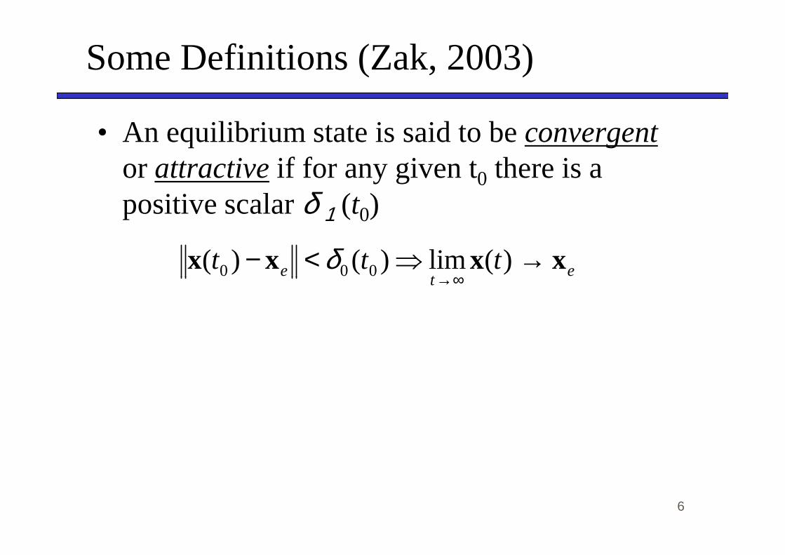
• An equilibrium state is said to be convergentor attractive if for any given t0 there is a positive scalar δ 1 (t0)
et
e ttt xxxx →⇒<−∞→
)(lim)()( 000 δ
6
et
e ∞→000

Some Definitions (Zak, 2003)
• An equilibrium state is asymptotically stable if stable and convergent
• An equilibrium state is uniformly stable if δ (t0,ε)= δ (ε)
• An equilibrium state is uniform convergent if • An equilibrium state is uniform convergent if δ 1 (t0) = δ 1
• An equilibrium state is uniformly asymptotically stable if is uniformly stable and uniformly convergent
7

Some Definitions (Zak, 2003)
• An equilibrium state xe is said to be unstable if there is an ε > 0 so that for any δ > 0 there exists x(t0) such that if
then
δ<− et xx )( 0
then
for some t1 > t0
8
ε≥− et xx )( 0

Some Definitions (Zak, 2003)
9

Some Definitions (Zak, 2003)
• Lyapunov’s Indirect Method
• Let the origin x=0 be an equilibrium state of the nonlinear system px=f(x). Then the origin is an asymptotically stable equilibrium of the nonlinear system if A, the Jacobianmatrix of nonlinear system if A, the Jacobianmatrix of f, evaluated at the origin, has all its eigenvalues in the open left-half plane.
• Take ECE675 for proof
10

Stability of Power Electronic Systems
• Reasons for concerns
• Subtleties
11

Physical Definition of Bus Stability
• A bus would be defined to be locally dynamically stable at a given operating condition provided that the bus voltage is constant at that operating point, and that if the bus voltage were perturbed it would return to
12
bus voltage were perturbed it would return to its original value
• Bus voltage is either dc, or q- and d-axis voltage in a synchronous reference frame
Practical Physical Def. of Bus Stability
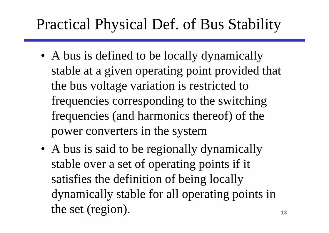
• A bus is defined to be locally dynamically stable at a given operating point provided that the bus voltage variation is restricted to frequencies corresponding to the switching frequencies (and harmonics thereof) of the
13
frequencies (and harmonics thereof) of the power converters in the system
• A bus is said to be regionally dynamically stable over a set of operating points if it satisfies the definition of being locally dynamically stable for all operating points in the set (region).
Physical Definition of System Stability
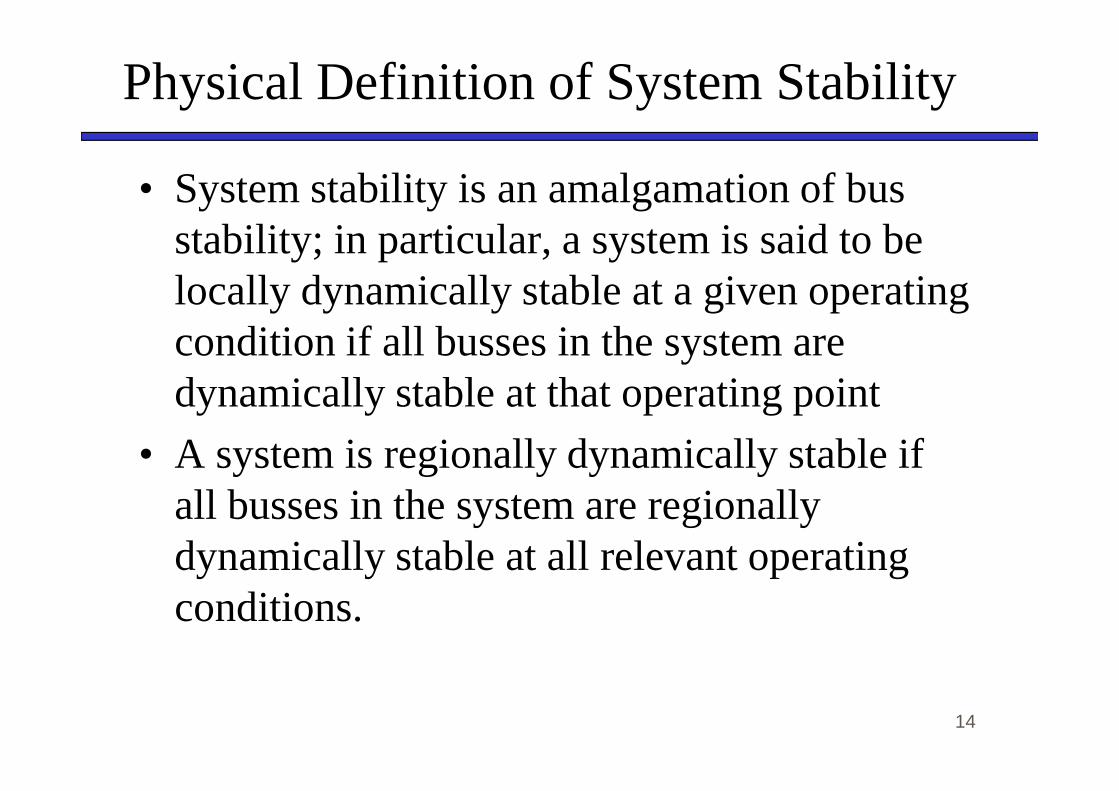
• System stability is an amalgamation of bus stability; in particular, a system is said to be locally dynamically stable at a given operating condition if all busses in the system are dynamically stable at that operating point
14
dynamically stable at that operating point
• A system is regionally dynamically stable if all busses in the system are regionally dynamically stable at all relevant operating conditions.

Consider a System
IMControls
Vol. Reg./Exciter
iabcsvdci
vdcsvr
ωrm,im
Te,desvdcs*
15
SM IMTurbineMechanical
Load
vdci
3 - Uncontrolled
Rectifier
φ 3 - Fully Controlled
Inverter
φLCFilter
CapacitiveFilter
Tie Line

System Performance
20
-20
ias, A *
16
100 ms
20
550
-20
250
ias, A
vdci, V

A Simple System
17

Linearizing…
18

Equivalent Circuit
19

Transfer Function
20

Characteristic Polynomial
21

A Condition for Stability
22

Another Condition for Stability
23

General Modeling Requirements
• We assume that all components can be represented in the following form
),( uxfx =
dt
d
∫=t
ττ1ˆ
24
dt
),( uxgy =
∫−
=t
Tt
dxT
x ττ )(1ˆ
Model Linearization
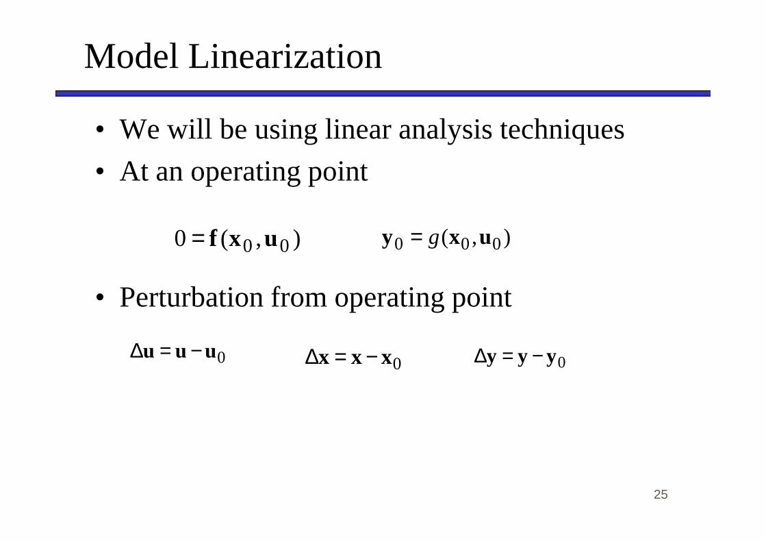
• We will be using linear analysis techniques
• At an operating point
),(0 00 uxf= ),( 000 uxy g=
25
• Perturbation from operating point
0uuu −=∆0xxx −=∆ 0yyy −=∆
Model Linearization
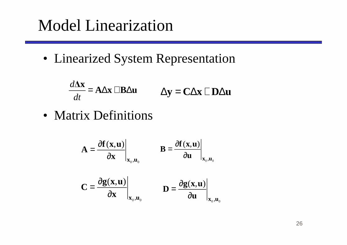
• Linearized System Representation
• Matrix Definitions
uBxA∆x ∆+∆=dt
duDxCy ∆+∆=∆
26
00,
),(
uxxuxf
A∂
∂=00,
),(
uxuuxf
B∂
∂=
00,
),(
uxxuxg
C∂
∂=00,
),(
uxuuxg
D∂
∂=

Writing Specification to Address Stability
27

Immittance from Linearized Models
• Going to the frequency domain
DBAIC +−= −1)()( ssI
28
Contour Evaluations of Complex Functions
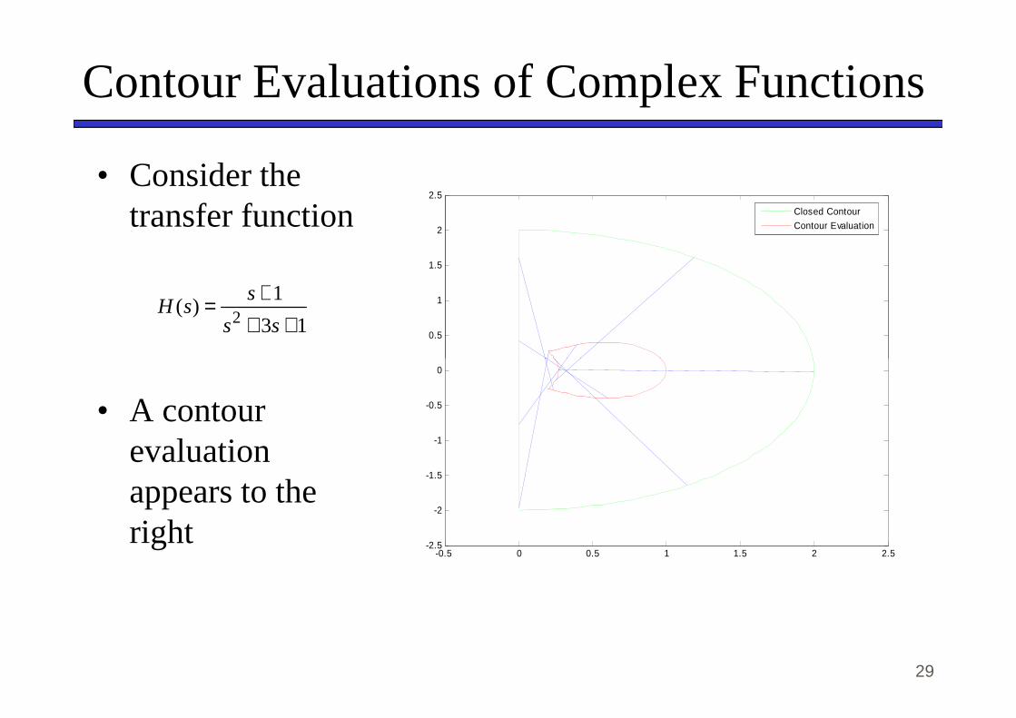
• Consider the transfer function
13
1)(
2 +++=
ss
ssH
0.5
1
1.5
2
2.5
Closed Contour
Contour Evaluation
29
• A contour evaluation appears to the right
-0.5 0 0.5 1 1.5 2 2.5-2.5
-2
-1.5
-1
-0.5
0
The Cauchy Principal
• A contour evaluation of a complex function will only encircle the origin if the contour contains a singularity of that function
30

Cauchy Principal: Example 1
)1)(1(
5.0)(
+−+=
ss
ssH
0.5
1
1.5
Closed Contour
Contour Evaluation
31
-1.5 -1 -0.5 0 0.5 1 1.5 2 2.5 3 3.5 4-1.5
-1
-0.5
0

Cauchy Principal: Example 2
)1)(1(
5.0)(
+−+=
ss
ssH
0.5
1
1.5
Closed Contour
Contour Evaluation
32
-1.5 -1 -0.5 0 0.5 1 1.5 2 2.5 3 3.5 4-1.5
-1
-0.5
0
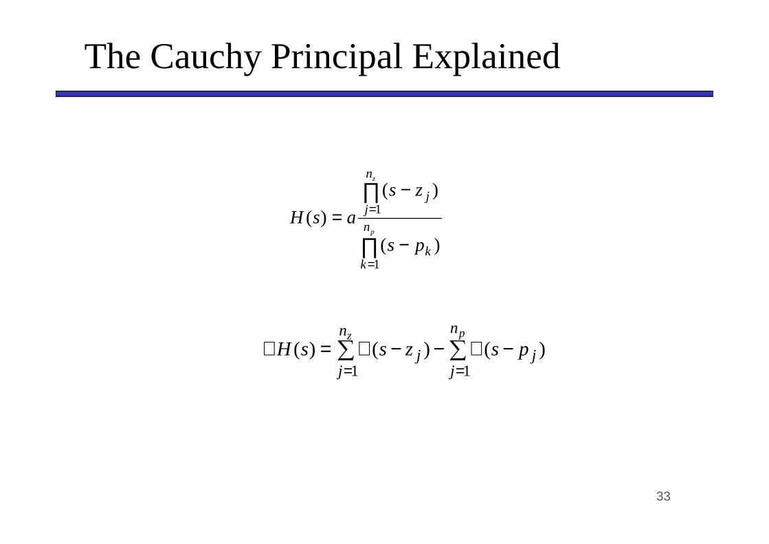
The Cauchy Principal Explained
∏
∏
=
=
−
−=
p
z
n
kk
n
jj
ps
zs
asH
1
1
)(
)(
)(
33
∑ ∑= =
−∠−−∠=∠z pn
j
n
jjj pszssH
1 1)()()(

The Cauchy Principal: Zeros
34

The Cauchy Principal: Poles
35
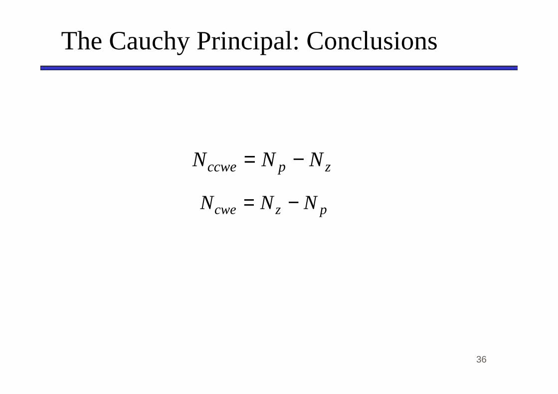
The Cauchy Principal: Conclusions
zpccwe NNN −=
NNN −=
36
pzcwe NNN −=
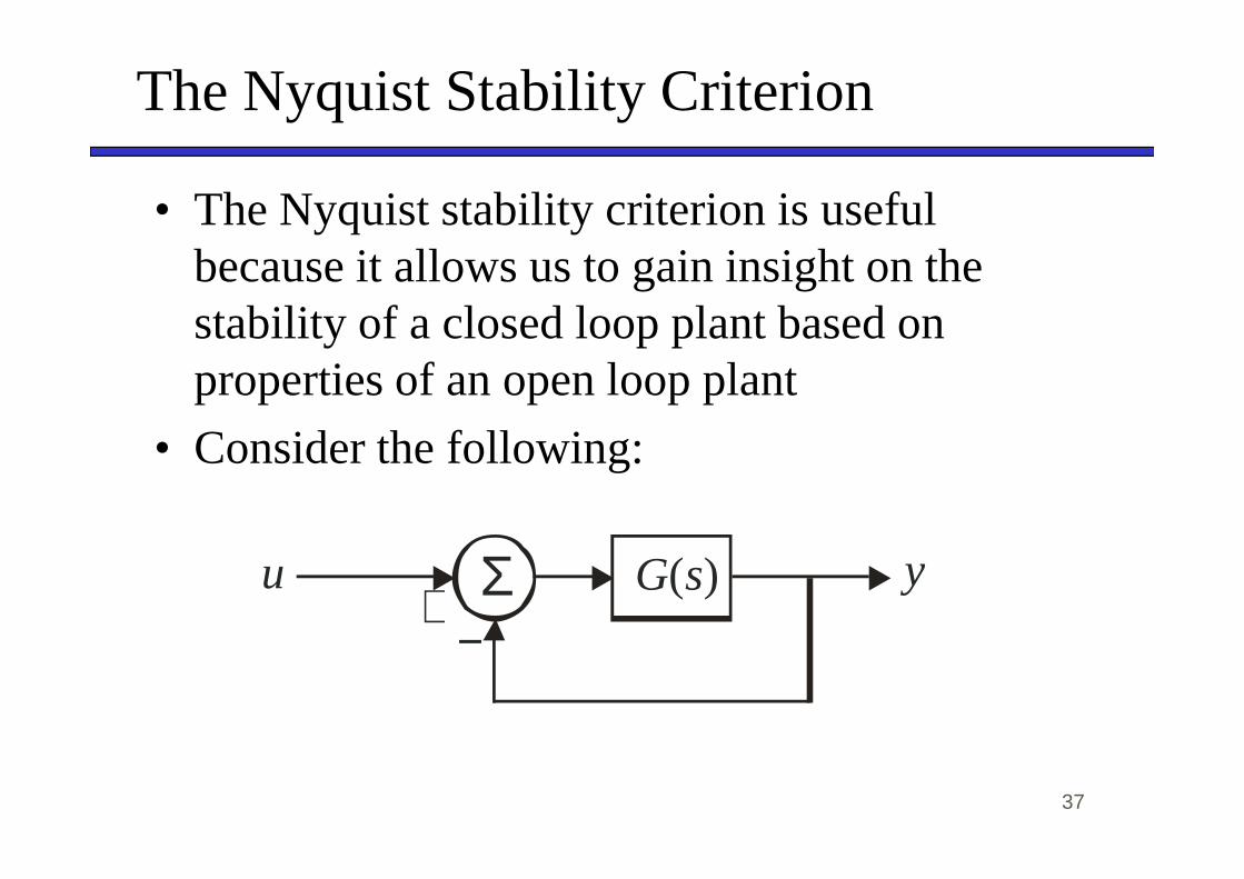
The Nyquist Stability Criterion
• The Nyquist stability criterion is useful because it allows us to gain insight on the stability of a closed loop plant based on properties of an open loop plant
• Consider the following:
37
• Consider the following:
)(sGΣ+−
yu

Nyquist Stability Criterion (Cont)
)(sGΣ+−
yu
38

Nyquist Stability Criterion (Cont)
39

The Nyquist Contour
∞j
∞
40∞− j

Nyquist Stability Criterion
• Consider a Nyquist evaluation of
• We have
)(1 sG+
pzcwe NNN −=
uclpz NN =
41
• Thus we have …
uclpz
uolpp NN =
uolpcweuclp NNN +=
Nyquist Stability Criterion
Nyquist Stability Criterion: The number of unstable closed loop poles is equal to the number of unstable open loop poles plus the number of clockwise encirclements of -1 by the contour evaluation of the open loop plant (i.e. G(s)) over
42
evaluation of the open loop plant (i.e. G(s)) over the Nyquist contour.

Comments on Path
max|| ω=s
maxωjs =
Point 2
Point 3
Point 4
43
maxωjs −=
maxω=s0=s
Point 1
Point 2 Point 4
s-plane
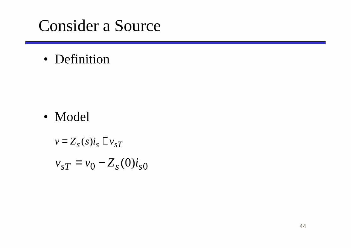
Consider a Source
• Definition
• Model
44
sTss visZv += )(
00 )0( sssT iZvv −=

Consider a Load
• Definition
• Model
45
lNll ivsYi += )(
00 )0( vYii lllN −=
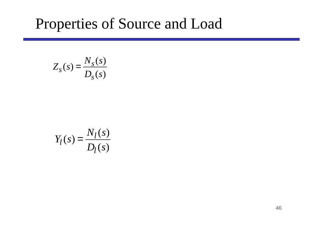
Properties of Source and Load
)(
)()(
sD
sNsZ
s
ss =
46
)(
)()(
sD
sNsY
l
ll =

Consider a Source-Load System
sZ
lYvsTv lNi
si li
++
--
Source Load
47
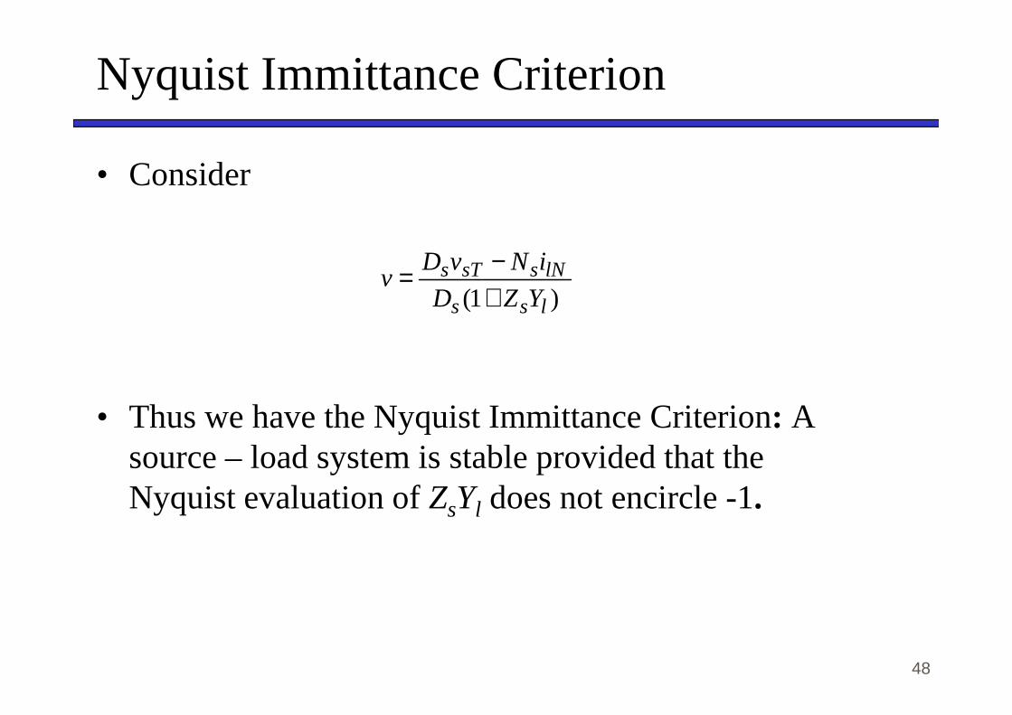
Nyquist ImmittanceCriterion
• Consider
)1( lss
lNssTs
YZD
iNvDv
+−=
48
• Thus we have the Nyquist Immittance Criterion: A source – load system is stable provided that the Nyquist evaluation of ZsYl does not encircle -1.

Quick Review – Gain and Phase Margin
49

Stability Criteria
1/GM
ImaginaryAxis
Unit CircleESACCriterion
GMPMCriterion
50
OpposingArgumentCriterion
PM 1/GM
Real Axis
Middlebrook Criterion
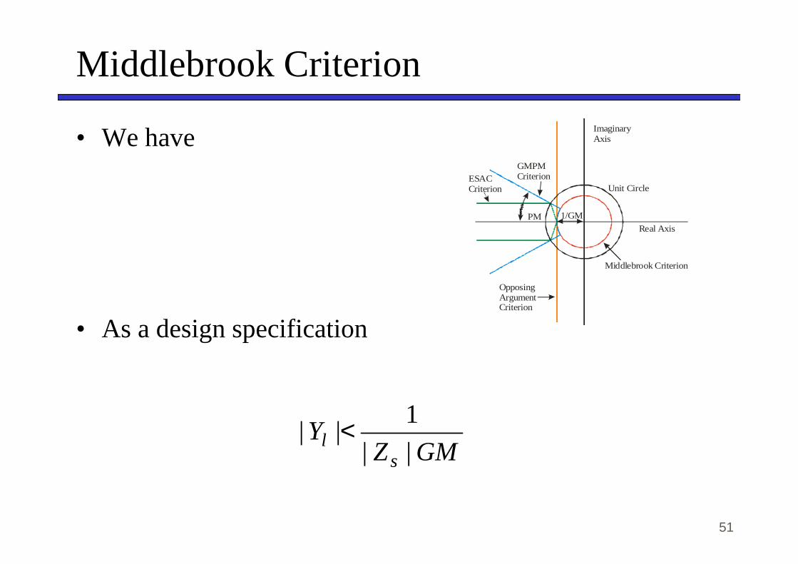
MiddlebrookCriterion
• We have
PM 1/GM
ImaginaryAxis
Unit Circle
Real Axis
Middlebrook Criterion
ESACCriterion
GMPMCriterion
51
• As a design specification
GMZY
sl ||
1|| <
OpposingArgumentCriterion
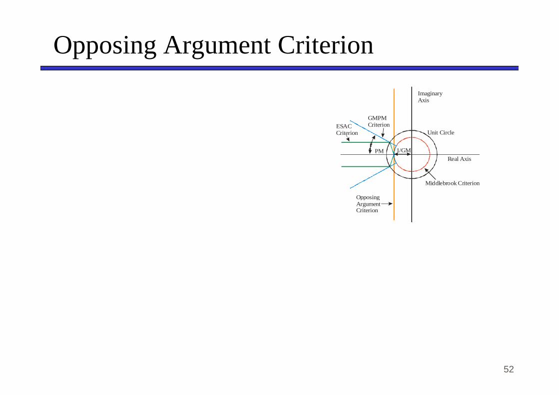
Opposing Argument Criterion
Opposing
PM 1/GM
ImaginaryAxis
Unit Circle
Real Axis
Middlebrook Criterion
ESACCriterion
GMPMCriterion
52
OpposingArgumentCriterion

Gain and Phase Margin Criterion
GMZY
sl ||
1|| <
Opposing
PM 1/GM
ImaginaryAxis
Unit Circle
Real Axis
Middlebrook Criterion
ESACCriterion
GMPMCriterion
- OR -
53
( )( )PMsZsY
PMsZsY
osl
osl
+−≥∠+∠
−≤∠+∠
∠
∠
180)()(
and180)()(
OpposingArgumentCriterion
- OR -

ESAC Criteria
PM 1/GM
ImaginaryAxis
Unit Circle
Real Axis
Middlebrook Criterion
ESACCriterion
GMPMCriterion
54
OpposingArgumentCriterion
Middlebrook Criterion
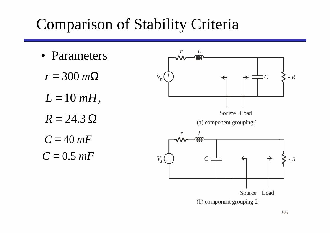
Comparison of Stability Criteria
• Parameters+_ C - R
Source Load
Vs
r L
Ω= mr 300
,10mHL =
Ω= 3.24R
55
+_ C - R
Source Load
Vs
r L
(a) component grouping 1
(b) component grouping 2
Ω= 3.24R
mFC 40=mFC 5.0=

Component Grouping A
ESACCriteria
Nyquist Contour,Stable Case
ImaginaryAxis
Arcs at |s| =
3
400π
56
GMPMCriteria
Criteria
Real Axis
Nyquist Contour,Unstable Case
|s| =
3
-3
-3
400π

Component Grouping B
ImaginaryAxis
ESAC Criteria
GMPMCriiteria
1.5
57
Nyquist ContourStable Case
Nyquist ContourUnstable Case
Real Axis
ESAC Criteria
-3
-1.5

Design Specs From Arb. Stab. Crit.
• At a frequency at a point
Nyquist Evaluationof Source Impedance
Zs,a
58
ESAC Stability Criteria
Real Axis
ImaginaryAxis
Zs,a
sbsc
sdas
babl Z
sY
,, =
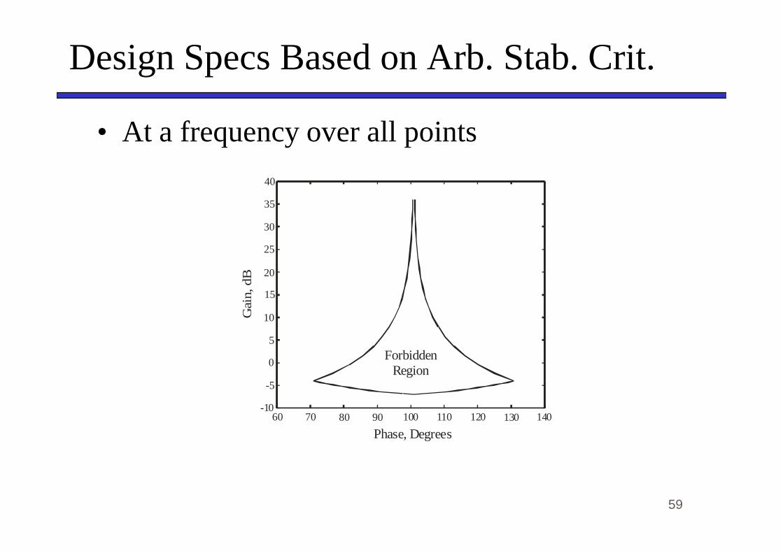
Design Specs Based on Arb. Stab. Crit.
• At a frequency over all points
Gain
, dB
40
35
30
25
20
59
Gain
, dB
Phase, Degrees
20
15
10
5
0
-5
-1060 70 80 90 100 110 120 130 140
ForbiddenRegion

Design Specs Based on Arb. Stab. Crit.
• Over all frequencies
60
40
20
ma
gn
itude
, d
B
Stability Constraint in Admittance Space
60
20
0
-20
-40300
200
100
00
-2
24
log of frequency, Hzphase, degrees
ma
gn
itude
, d
B
Inflection
Load Admittance,Unstable Case
Load Admittance,Stable Case

Comments
• Conservativeness
• Amenability to Configuration
61
• Simplicity of Formulating Design Specs

Generalized Immittance
• Consider the following system
IMControls
Vol. Reg./Exciter
iabcsvdcsvr
ωrm,im
Te,desvdcs*
62
SM IMTurbineMechanical
Load
iabcsvdci
vdcsvr
3 - Uncontrolled
Rectifier
φ 3 - Fully Controlled
Inverter
φLCFilter
CapacitiveFilter
Tie Line

Source Impedance Vs. Operating Point
• Output Power from 0 to 1 p.u. in 5 steps
20
40
60
mag
nitu
de,
dB
63
-2-1
01
23
-100
0
100-40
-20
0
20
log of frequency, Hzphase, degrees
mag
nitu
de,
dB
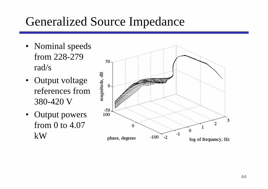
Generalized Source Impedance
• Nominal speeds from 228-279 rad/s
• Output voltage references from
64
references from 380-420 V
• Output powers from 0 to 4.07 kW
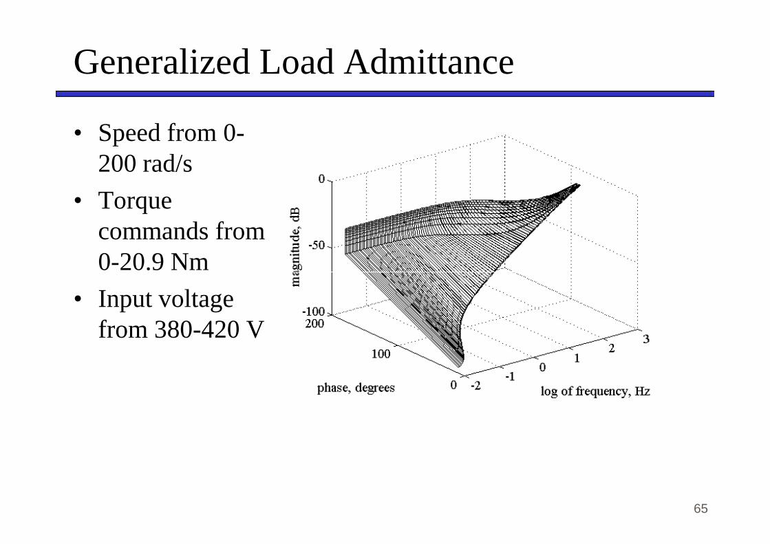
Generalized Load Admittance
• Speed from 0-200 rad/s
• Torque commands from 0-20.9 Nm
65
0-20.9 Nm
• Input voltage from 380-420 V

Generalized Nyquist Evaluation
• Source Impedance
• Load Admittance
)()( sZsZ G⇒
66
)()( sYsY G⇒

Product of Generalized Quantities
• Consider
)()( sXsx G∈ )()( sYsy G∈
67

Implications on Stability
• Consider Nyquist Evaluation of )()( sYsZ GG
68

An Example
• Consider the followingΩ= 3.97loadR
Ω= 3.24loadR
0.3 Ω 5 mH
69
+_ 500 Fµ - Rload
Source Load
vs
0.3 Ω 5 mH

Normal Nyquist
1
UnstableCase
70
-2 -1
-1
0StableCase

Let’s Add Variation
• Allow all parameters to vary by 1%1
1|)()( ωjs
Gl
Gs sYsZ =
71
-2 -10
-1

Generalized Middlebrook
• Standard Middlebrook
• Generalized MiddlebookGMsYsZ ls
1)()( <
xX = max
72
GXxG
xX∈
= max
GMsYsZG
Gl
G
Gs /1)()( <

Generalized Middlebrook
• In terms of design specs:• If we know source
G
Gs
G
Gl
sZGMsY
)(
1)( <
73
• If we know load
G
Gs
G
Gl
sYGMsZ
)(
1)( <

Generalizing Other Criteria
Nyquist Evaluationof NominalSource Impedance
sbsc
PasZ ,
GasZ ,
absZ ,
ε
abs
babl Z
SY
,, =
74
ESAC Stability Criteria
Real Axis
ImaginaryAxis
sc
sd
εbt
∫ −P
asZas
abs
bb dssZ
Z
st
,
)(,,
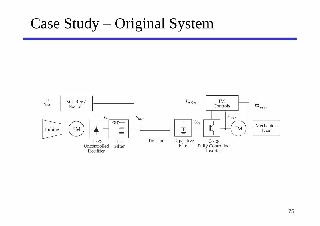
Case Study – Original System
IMControls
Vol. Reg./Exciter ωrm,im
Te,desvdcs*
75
SM IMTurbineMechanical
Load
iabcsvdci
vdcsvr
3 - Uncontrolled
Rectifier
φ 3 - Fully Controlled
Inverter
φLCFilter
CapacitiveFilter
Tie Line

Gen. Adm. Constraint and Admittance
76

Original System Time Domain Perform.
20
20
-20
ias, A *
77
100 ms
20
550
-20
250
ias, A
vdci, V

Let’s Modify the Control
78

Modified Control
79

Adm. Constraint and Modified Adm
80
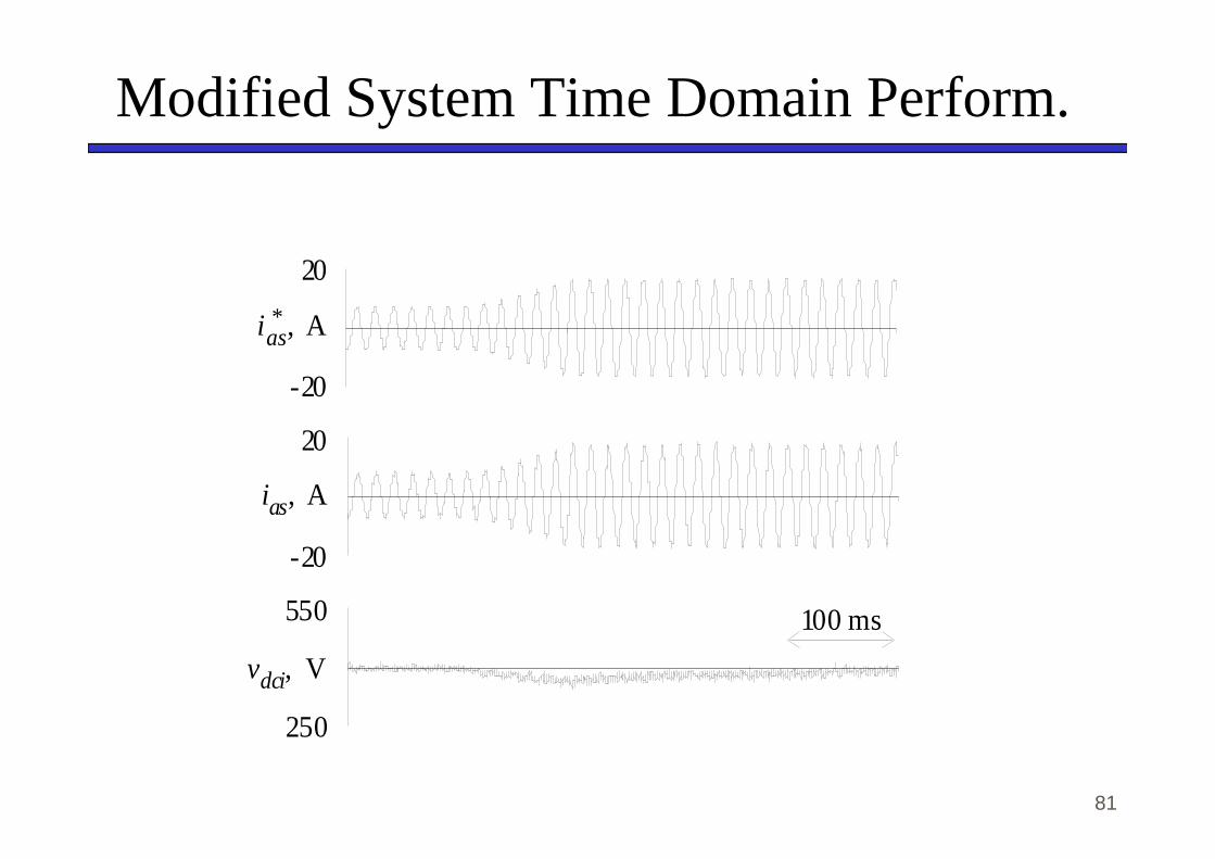
Modified System Time Domain Perform.
20
20
-20
ias, A *
81
100 ms
20
550
-20
250
ias, A
vdci, V