stability of high speed train under aerodynamic...

Stability of High Speed Train under AerodynamicExcitations

Master’s Thesis in Solid and Fluid Mechanics

ERIK BJERKLUND

MIKAEL OHMAN

Department of Applied MechanicsDivision of Dynamics and Division of Fluid MechanicsCHALMERS UNIVERSITY OF TECHNOLOGYGoteborg, Sweden 2009Master’s Thesis 2009:03

MASTER’S THESIS 2009:03

Stability of High Speed Train under Aerodynamic Excitations

Master’s Thesis in Solid and Fluid MechanicsERIK BJERKLUNDMIKAEL OHMAN

Department of Applied MechanicsDivision of Dynamics and Division of Fluid Mechanics

CHALMERS UNIVERSITY OF TECHNOLOGY

Goteborg, Sweden 2009

Stability of High Speed Train under Aerodynamic ExcitationsERIK BJERKLUNDMIKAEL OHMAN

c©ERIK BJERKLUND, MIKAEL OHMAN, 2009

Master’s Thesis 2009:03ISSN 1652-8557Department of Applied MechanicsDivision of Dynamics and Division of Fluid MechanicsChalmers University of TechnologySE-412 96 GoteborgSwedenTelephone: + 46 (0)31-772 1000

Cover:Train leaving a tunnel and is hit by a strong side wind.

Chalmers ReproserviceGoteborg, Sweden 2009

Stability of High Speed Train under Aerodynamic ExcitationsMaster’s Thesis in Solid and Fluid MechanicsERIK BJERKLUNDMIKAEL OHMANDepartment of Applied MechanicsDivision of Dynamics and Division of Fluid MechanicsChalmers University of Technology

Abstract

It is important to study the aerodynamic effects on high speed trains, due to bothcomfort and stability. The Swedish high speed trains are aiming to go at a speedof 250 km/h. The present work closely connects the aerodynamic effects with thevibration dynamics within the train.

Two scenarios are simulated, two trains meeting each other and a train leavinga tunnel and is hit by a strong wind gust (35 m/s). From the aerodynamic part,computational fluid dynamics (CFD) is used with the k-ζ-f turbulence model. Tosimulate both scenarios a moving mesh needs to be used. From the CFD the momentsand forces from the pressure and traction on the train body are calculated, and theseloads are taking into a low order mathematical model that simulates the vibrationdynamics in the train.

For the scenario with meeting trains the train experiences some slight vibrations,causing discomfort, but has no impact on the stability of the train, but for thescenario with the tunnel and side wind the train has a very high risk of derailment.

From the results of the dynamics simulations a comfort and stability measure-ments were constructed based on the vibrations in the train car and the risk of wheelclimbing. From simulating different speeds of the train it could be seen that thecomfort and stability change linearly with the speed. Work was also done to seehow much impact the coupling between the car bodies can have on the comfort andstability. A comparison was made to a simple, stiff coupling and one that optimizesa set of passive dampers. It’s seen that the coupling can make a difference of around8% in comfort and stability, which equals an effect of lowering the speed 3-5 m/s.

Semi-active dampers of sky-hook and ground-hook type were also tested in thecoupling, but they only showed insignificant changes or changes to the worse.

Keywords: Moving mesh, Wind loads, Coupling, Vibration dynamics, CFD, High speedtrain, Comfort, Stability

, Applied Mechanics, Master’s Thesis 2009:03 I

II , Applied Mechanics, Master’s Thesis 2009:03

Contents

Abstract I

Contents III

Preface V

1 Introduction 11.1 Purpose . . . . . . . . . . . . . . . . . . . . . . . . . . . . . . . . . . . . . 11.2 Limitations . . . . . . . . . . . . . . . . . . . . . . . . . . . . . . . . . . . 11.3 Approach . . . . . . . . . . . . . . . . . . . . . . . . . . . . . . . . . . . . 1

2 Theory of Aerodynamic Simulations 22.1 Turbulence Models . . . . . . . . . . . . . . . . . . . . . . . . . . . . . . . 32.2 Coefficients and Mesh Quality Measurements . . . . . . . . . . . . . . . . . 5

3 Theory of Vibration Dynamics 63.1 Wind Load . . . . . . . . . . . . . . . . . . . . . . . . . . . . . . . . . . . 73.2 Contact Forces . . . . . . . . . . . . . . . . . . . . . . . . . . . . . . . . . 8

3.2.1 Contact Patch Dimensions . . . . . . . . . . . . . . . . . . . . . . . 93.2.2 Wheel Forces from Creep . . . . . . . . . . . . . . . . . . . . . . . . 10

3.3 Statement of the Vibrational Problem . . . . . . . . . . . . . . . . . . . . . 103.3.1 Cost Function for Stability . . . . . . . . . . . . . . . . . . . . . . . 113.3.2 Cost Function for Comfort . . . . . . . . . . . . . . . . . . . . . . . 12

4 Method for Aerodynamic Simulations 124.1 Mesh Creation . . . . . . . . . . . . . . . . . . . . . . . . . . . . . . . . . . 12

4.1.1 Mesh Topology for the Two Meeting Trains . . . . . . . . . . . . . 134.1.2 Mesh Topology for the Train Exiting a Tunnel . . . . . . . . . . . . 15

4.2 Mesh Deformation . . . . . . . . . . . . . . . . . . . . . . . . . . . . . . . 154.3 Setup of CFD Solver . . . . . . . . . . . . . . . . . . . . . . . . . . . . . . 17

5 Method for Vibration Dynamic Simulations 185.1 Bogie model . . . . . . . . . . . . . . . . . . . . . . . . . . . . . . . . . . . 18

5.1.1 Degrees of Freedom . . . . . . . . . . . . . . . . . . . . . . . . . . . 185.1.2 Geometry of Bogie . . . . . . . . . . . . . . . . . . . . . . . . . . . 205.1.3 Placement of Springs and Dampers . . . . . . . . . . . . . . . . . . 20

5.2 Optimization of the Coupling . . . . . . . . . . . . . . . . . . . . . . . . . 245.3 Computational Model . . . . . . . . . . . . . . . . . . . . . . . . . . . . . 24

5.3.1 Choice of the ODE Solver . . . . . . . . . . . . . . . . . . . . . . . 255.3.2 Automatic Construction of the Stiffness Matrices . . . . . . . . . . 25

6 Results from Aerodynamic Simulations 266.1 Two Trains Meeting at High Speed . . . . . . . . . . . . . . . . . . . . . . 266.2 Train Exiting a Tunnel under Influence of a Wind Gust . . . . . . . . . . . 326.3 Discussion of CFD method and results . . . . . . . . . . . . . . . . . . . . 36

7 Results from Vibration Dynamic Simulations 377.1 Optimization of the Coupling . . . . . . . . . . . . . . . . . . . . . . . . . 387.2 Coupling Sky-hook . . . . . . . . . . . . . . . . . . . . . . . . . . . . . . . 42

, Applied Mechanics, Master’s Thesis 2009:03 III

8 Conclusions 42

9 Recommendations 43

IV , Applied Mechanics, Master’s Thesis 2009:03

Preface

In this study the forces from aerodynamic simulations have been used to analyze thevibrational behaviour of a high speed train in respect to comfort and stability. A scenarioof two trains meeting and a scenario of a train leaving a tunnel with a strong side windare simulated. The work has been carried out from September 2008 to April 2009 at theDepartment of Applied Mechanics, Division of Dynamics and Division of Fluid Mechanics,Chalmers University of Technology, Sweden, with Mikael ı¿1

2hman as student and Professor

Viktor Berbyuk as supervisor for the vibration dynamics and Erik Bjerklund as studentand Associate Professor Sinisa Krajnovic as supervisor for the fluid mechanics.

Aknowledgements

We would like to say our thanks to our supervisors and the department of Applied Me-chanics for their support, to Albin Jonsson for his help with the vibration dynamics and tothe CFD support at AVL, Dr. Branislav Basara, Andreas Diemath and Jurgen Schneider.A special thanks to AVL for providing the Fire licenses. Without their help this projectwould not have been possible.

Goteborg April 2009Erik Bjerklund, Mikael Ohman

, Applied Mechanics, Master’s Thesis 2009:03 V

VI , Applied Mechanics, Master’s Thesis 2009:03

1 Introduction

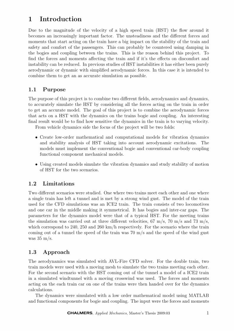
Due to the magnitude of the velocity of a high speed train (HST) the flow around itbecomes an increasingly important factor. The unsteadiness and the different forces andmoments that start acting on the train have a big impact on the stability of the train andsafety and comfort of the passengers. This can probably be countered using damping inthe bogies and coupling between the trains. This is the reason behind this project. Tofind the forces and moments affecting the train and if it’s the effects on discomfort andinstability can be reduced. In previous studies of HST instabilities it has either been purelyaerodynamic or dynamic with simplified aerodynamic forces. In this case it is intended tocombine them to get an as accurate simulation as possible.

1.1 Purpose

The purpose of this project is to combine two different fields, aerodynamics and dynamics,to accurately simulate the HST by considering all the forces acting on the train in orderto get an accurate model. The goal of this project is to combine the aerodynamic forcesthat acts on a HST with the dynamics on the trains bogie and coupling. An interestingfinal result would be to find how sensitive the dynamics in the train is to varying velocity.

From vehicle dynamics side the focus of the project will be two folds:

• Create low-order mathematical and computational models for vibration dynamicsand stability analysis of HST taking into account aerodynamic excitations. Themodels must implement the conventional bogie and conventional car-body couplingfunctional component mechanical models.

• Using created models simulate the vibration dynamics and study stability of motionof HST for the two scenarios.

1.2 Limitations

Two different scenarios were studied. One where two trains meet each other and one wherea single train has left a tunnel and is met by a strong wind gust. The model of the trainused for the CFD simulations was an ICE2 train. The train consists of two locomotivesand one car in the middle making it symmetrical. It has bogies and inter-car gaps. Theparameters for the dynamics model were that of a typical HST. For the meeting trainsthe simulation was carried out at three different velocities, 67 m/s, 70 m/s and 73 m/s,which correspond to 240, 250 and 260 km/h respectively. For the scenario where the traincoming out of a tunnel the speed of the train was 70 m/s and the speed of the wind gustwas 35 m/s.

1.3 Approach

The aerodynamics was simulated with AVL-Fire CFD solver. For the double train, twotrain models were used with a moving mesh to simulate the two trains meeting each other.For the second scenario with the HST coming out of the tunnel a model of a ICE2 trainin a simulated windtunnel with a moving crosswind was used. The forces and momentsacting on the each train car on one of the trains were then handed over for the dynamicscalculations.

The dynamics were simulated with a low order mathematical model using MATLABand functional components for bogie and coupling. The input were the forces and moments

, Applied Mechanics, Master’s Thesis 2009:03 1

calculated from the CFD simulations and the forces acting on the wheels from the rail.Unknown parameters, such as damping coefficients in the bogie, were decided by minimiz-ing a cost function for comfort and stability. As a last step, active damping was added tothe model.

2 Theory of Aerodynamic Simulations

To solve the flow around the trains CFD was used. CFD is based on the finite volumeapproach. This means that the conservational principals are applied for the propertiesdescribing the behaviour of a matter interacting with its surrounding. The laws of conser-vation of mass and momentum for a finite volume gives the continuity equation (2.1) andthe equation of motion (2.2).

∂ρ

∂t+

∂

∂xi(ρui) = 0 (2.1)

ρ

(∂ui∂t

+ uj∂ui∂xj

)= ρbi +

∂σij∂xj

(2.2)

σij = −pδij + λδij∂ui∂xi

+ µ

(∂ui∂xj

+∂uj∂xi

)(2.3)

Combining these together with the constitutive equations and assuming Stokes condi-tion (λ = −2

3µ) for an isotropic homogeneous Newtonian fluid (2.3), which air is, one ends

up with the instantaneous compressible Navier-Stokes equations (2.4).

ρ

(∂ui∂t

+ uj∂ui∂xj

)= ρbi −

∂p

∂xi+

∂

∂xj

[µ

(∂ui∂xj

+1

3

∂uj∂xi

)](2.4)

The Navier-Stokes equations are non-linear partial differential equations and believedto precisely describe any type of flow. However only a few exact solutions exists so theNavier-Stokes equations have to be solved numerically. This is easier done by splitting upthe instantaneous variables into a mean and a fluctuating part.

r =1

T

∫T

r(t)dt = R

r =R + r

This is called Reynolds decomposition and the resulting equations are called Reynolds-averaged Navier-Stokes equations (2.5) (RANS). Note that no incompressibility assumptionwere done in this project.

ρ

(∂Ui∂t

+ Uj∂Ui∂xj− ui

∂uj∂xj

)=

ρbi −∂P

∂xi+

∂

∂xj

[µ

(∂Ui∂xj

+1

3

∂Uj∂xi

)− ρuiuj

](2.5)

The decomposition leads to a few extra terms, which lead to more unknowns thanequations. This is known as the turbulence closure problem and in order to solve theequations the terms has to be modelled.

2 , Applied Mechanics, Master’s Thesis 2009:03

Table 2.1: Explanation of variables used in continuum mechanics.t Timep Pressureui Velocity vectorxi Coordinate vectorbi Body force vectorµ Viscosityλ Bulk viscosityρ Densityσij Stress tensorδij Kronecker deltar Arbitrary instantaneous variable

2.1 Turbulence Models

Two important components of turbulent flow is the kinetic energy k and the dissipation ε.

k =1

2uiui (2.6)

ε =ν∂ui∂xj

∂ui∂xj

(2.7)

The Boussinesq eddy viscosity assumption is that there is an turbulent viscosity thatcan linearly describe the turbulent flow structures. For the k-ε model the assumption is

νt =µtρ

= Cµk2

ε(2.8)

Using an eddy viscosity model as k-ε the kinetic energy and the dissipation are calcu-lated by solving the modelled transport equations (2.9) numerically.

dk

dt= Pk − ε+B +

1

ρ

∂

∂xj

[(µ+

µtσk

)∂k

∂xj

]dε

dt=

(Cε1Pk − Cε2ε+ Cε3B +

1

3k∂Uk∂xk

)ε

k+

1

ρ

∂

∂xj

[(µ+

µtσε

)∂ε

∂xj

] (2.9)

where

Pk = νt

(∂Ui∂xj− ∂Uj∂xi

)(∂Ui∂xj− ∂Uj∂xi

)− 2

3

(νt∂Uk∂xk

+ k

)∂Uk∂xk

(2.10)

B = −biµtσρ

∂ρ

∂xi(2.11)

The body force term bi is neglected in this case because of the cold flow. The coefficientsused have the following standard values given in table 2.2 [1].

Table 2.2: Coefficients for the k-ε model.Cµ Cε1 Cε2 Cε3 σk σε σρ

0.09 1.44 1.92 0.8 1 1.3 0.9

Another eddy-viscosity model used in this project is the k-ζ-f model [8]. It is analtered version of a v2-f model for numerical stability, where special treatment of the wall


normal stress v2 is taken. This in order to improve the modeling of the wall effects on the

turbulence. The new variable ζ is the velocity scale ratio ζ =v2

k. This variable get its own

transport equation to be solved. The eddy viscosity in the k-ζ-f model is obtained from

νt = Cµζkτ (2.12)

and the transport equations are

dk

dt= Pk − ε+

1

ρ

∂

∂xj

[(µ+

µtσk

)∂k

∂xj

]dε

dt= (C∗ε1Pk − Cε2ε)

1

τ+

1

ρ

∂

∂xj

[(µ+

µtσε

)∂ε

∂xj

]dζ

dt= f − Pk

ζ

k+

1

ρ

∂

∂xj

[(µ+

µtσζ

)∂ζ

∂xj

]

(2.13)

The function f is obtained by solving

L2 ∂2f

∂xj∂xj− f =

(Cf1 + Cf2

Pkε

)(ζ − 2

3

)1

τ(2.14)

The turbulent time scale τ and length scale L are given by

τ = max

[min

[k

ε,

a√6Cµ|S|ζ

], Cτ

(νε

)1/2]

(2.15)

L = CL max

[min

[k3/2

ε,

k1/2

√6Cµ|S|ζ

], Cη

(ν3

ε

)1/4]

(2.16)

The coefficient C∗ε1 are modified in the ε equation by dampening the coefficient closeto the wall

C∗ε1 = Cε1 (1 + 0.012/ζ) (2.17)

The value of the coefficients shown in table 2.3 are all based on empirical studies [8].

Table 2.3: Coefficients for the k-ζ-f model.Cµ Cε1 Cε2 Cf1 Cf2 σk σε σζ Cτ CL Cη

0.22 1.4 1.9 0.4 0.65 1 1.3 1.2 6.0 0.36 85


Table 2.4: Explanation of variables used in the turbulence models.t Timep Pressureui Velocity vectorxi Coordinate vectorbi Body force vectork Kinetic energyPk Productionε Dissipationµ Viscosityµt Turbulent viscosityν Kinematic viscosityνt Turbulent kinematic viscosityρ Densityζ Velocity scale ratiof Function implicitly defined by itselfL Length scaleτ Time scaleS Strain rate tensorσ∗ Model coefficientC∗ Model coefficient

2.2 Coefficients and Mesh Quality Measurements

The force and moment coefficients are calculated as

CF =F

ρAu2/2(2.18)

CM =M

ρALu2/2(2.19)

where density used for scaling is ρ = 1.189 kg/m3, reference length L=3 m,the referencearea A=10 m2 and u is the speed of the train.

The standard procedure to check the quality of the calculations is to look at the dimen-sionless wall distance, y+ and the Courant number, C. The lower y+ the more resolvedthe flow is, which means more accurate results. The y+ is calculated as

y+ =u∗y

ν(2.20)

u∗ ≡√τwρ

(2.21)

τw = µ

(∂u

∂y

)y=0

(2.22)

where y is the height of the first cell from the wall.The Courant number of the flow is calculated as

C =u′∆t

h< 1 (2.23)

where u′ is the RMS of the velocity and h is the height of cell. The Courant number (CFLnumber) is supposed to be below one at all times in the entire mesh to ensure that theinformation travels from one cell to the next. The Courant number can however locally behigher without affecting the flow.


3 Theory of Vibration Dynamics

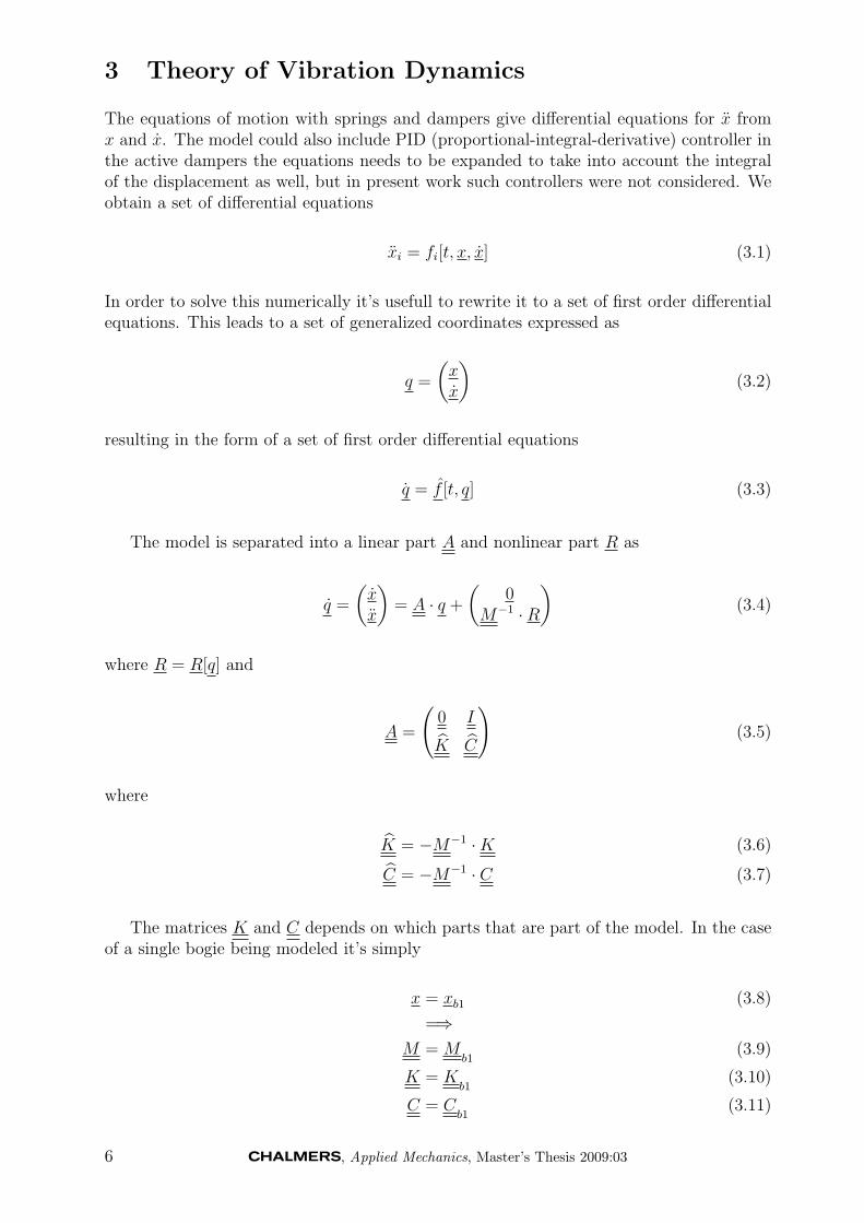
The equations of motion with springs and dampers give differential equations for x fromx and x. The model could also include PID (proportional-integral-derivative) controller inthe active dampers the equations needs to be expanded to take into account the integralof the displacement as well, but in present work such controllers were not considered. Weobtain a set of differential equations

xi = fi[t, x, x] (3.1)

In order to solve this numerically it’s usefull to rewrite it to a set of first order differentialequations. This leads to a set of generalized coordinates expressed as

q =

(xx

)(3.2)

resulting in the form of a set of first order differential equations

q = f [t, q] (3.3)

The model is separated into a linear part A and nonlinear part R as

q =

(xx

)= A · q +

(0

M−1 ·R

)(3.4)

where R = R[q] and

A =

(0 I

K C

)(3.5)

where

K = −M−1 ·K (3.6)

C = −M−1 · C (3.7)

The matrices K and C depends on which parts that are part of the model. In the caseof a single bogie being modeled it’s simply

x = xb1 (3.8)

=⇒M = M

b1(3.9)

K = Kb1

(3.10)

C = Cb1

(3.11)


and with a single train car with two bogies they are assembled as

x =

xc1xv1b1xv1b2

(3.12)

=⇒ (3.13)

M =

M c10 0

0 Mc1b1

0

0 0 Mc1b2

(3.14)

K =

Kc1

BKc1b1

BKc1b2

BKT

c1b1Kc1b1

0

BKT

c1b20 K

c1b2

(3.15)

C =

Cc1

BCc1b1

BCc1b2

BCT

c1b1Cc1b1

0

BCT

c1b20 C

c1b2

(3.16)

where 1 is for the train car, 2 for the front bogie and 3 for the back bogie and the matricesBK, BC are the coupling between the car and bogies.

In the simulations where no PID regulator is used, the system is simplified by reducingthe first row and first column of A.

The nonlinear forces, R, can be separated into a set of nonlinear forces

R = Rcontact +Rwind (3.17)

3.1 Wind Load

The wind load can be expressed as Rwind[t], or more suitable as Rwind[s[t]] where s[t] is thelocation of the train. Expressing the wind loads as a function of the location instead ofthe time will make it easier to interpolate over different absolute velocities. Interpolatingis only suitable if the set of CFD simulations over different train velocities is not to coarse,as the form of the forces and moments, F [s[t]], M [s[t]] should have a similar shape whenchanging the velocity a little as opposed to F [t] where the trains will pass each other faster.This can be seen in figure 6.12.

When simulating for a higher speed than available from the CFD simulations, extrap-olation is done by scaling through the drag, side and lift coefficient.

C =F [u]

12ρAu2

= constant =Fu0

12ρAu2

0

(3.18)

=⇒

F [u] =1

2ρAu2C = Fu0

(u

u0

)2

(3.19)

where u0 is the closest speed for which forces have been calculated. If the simulated speedis within the simulated domain the forces can be interpolated when expressed as functionsof the traveled distance.


3.2 Contact Forces

The contact forces are calculated from creep in the contact plane. The creep is defined as

ξx =Vwheel,xV0

(3.20)

ξη =Vwheel,ηV0

(3.21)

where x is in the longitudinal direction, η is perpendicular x and the normal at the contactpoint and V0 is the forward velocity of the train.

y

z

x

r0w0

η

Rail

Figure 3.1: Wheelset showing width and radius from center of gravity to nominal contactpoint.

Right side refers to the right in the forward direction of the train, i.e. the right wheelis shown in figure 3.1.

The velocities can now be calculated as

ω0 =V0

r0(3.22)

s =

+1 if right side

−1 if left side(3.23)

r = r[−sx2] (3.24)

w = sw0 − x2 (3.25)

d =

0wr

(3.26)

Rz

=

cos[−ϕ3] − sin[−ϕ3] 0sin[−ϕ3] cos[−ϕ3] 0

0 0 1

(3.27)

V wheel = x+

V0

00

+Rz· (d× (ϕ+

0ω0

0

)) (3.28)

where the r is an interpolating function of the geometry of a standardized S1002 wheelprofile [7].


Table 3.1: Explanation of variables for calculating the creep.x Translation vector of wheelset.ϕ Rotation vector of wheelset.r0 Wheel radius at nominal contact point.r Wheel radius at current contact point.w0 Lateral distance from COG to nominal contact point.w Lateral distance from COG to current contact point.V0 Nominal forward velocity of train.ω0 Nominal angular velocity of wheels.δ Inclination of wheels (positive).s Side dependence, +1 for right side, -1 for left side.

3.2.1 Contact Patch Dimensions

To calculate the forces the dimensions of the contact patch are required. According toHertz theory the dimensions are calculated as [4] and [7]

A+B =1

2

(1

rη,r+

1

rη,w+

1

rx,r+

1

rx,w

)(3.29)

B − A =1

2

((1

rx,r− 1

rη,r

)2

+

(1

rx,w− 1

rη,w

)2

+

2

(1

rx,r− 1

rη,r

)(1

rx,w− 1

rη,w

)cos[2φz]

) 12

(3.30)

Ψ = 3

√3N

2(A+B)

(1− ν2

w

Ew+

1− ν2r

Er

)(3.31)

θ = arccos

[B − AA+B

](3.32)

a =mΨ (3.33)

b =nΨ (3.34)

where m = m[θ] and n = n[θ]. There is no explicit expression for m[θ] or n[θ] but theycan be solved numerically with (4.25) through (4.32) in [11]. This has been done in table8-1 in [7] which values are used.

Table 3.2: Explanation of variables for calculating the creep.N Normal force in contact.

Ew, Er Modulus of elasticity in the wheel and rail.νw, νr Poissons ratio for the wheel and rail.a, b Contact patch dimension along x and η.

rx,w, rx,r, rη,w, rη,r Radius around the respective axis for wheel and rail.φz The angle of the wheel.

The radius rη,r is zero since the rail is straight. The other radii varies with the contactpoint and wheel profile. However they are approximated as constant for the contact geom-etry at a point far from the flange where the wheel is almost flat. In that case rx,w = ∞and rη,w = r. For the wheel the radius over the top of the rail is almost constant and beapproximated as rx,r = 300mm. In this case η-axis is parallell with the y-axis. The effect


from the rotation of the wheel is also neglected, as this angle will always be small, i.e.linearisation of cos[2φz] ≈ 1. This simplifies the equations and with the approximations ofthe radii the variables m and n are constant.

The rest of the material parameters were set to Ew = Er = 200 GPa and νw = νr = 0.3.

3.2.2 Wheel Forces from Creep

The creep forces are calculated with Kalker’s linear theory [7]. The coefficients for thecreep, C = C[a

b], are interpolated from a set of data taken from table 8-2 in [7].

F lin = −Gab(C11ξxC22ξη

)(3.35)

u =|F lin|µN

(3.36)

F = F lin

1− u

3+ u2

27if u < 3

µN|F lin|

otherwise(3.37)

The behaviour of the flange will be greatly simplified as done in [13]

Fflange =

kflange(nflange − x2) if x2 > nflange ∧ s > 0 (right side)

kflange(−nflange − x2) if x2 < −nflange ∧ s < 0 (left side)

0 otherwise

(3.38)

where Fflange acts in the y-axis and is added to Fy.

The force vector F is here acting on the contact plane, so to get the horizontal compo-nent

F =

(FxFy

)=

(F1

F2δ√

1+δ2+ Fflange

)(3.39)

The contributions to the nonlinear force on the system will be

Re =

FxFy00rFx

−wFx − wFy sin[φ3]

(3.40)

which is assembled into R for each wheel.

3.3 Statement of the Vibrational Problem

The problem is divided into two parts, handled separately, stability and comfort. It isnecessary to define a single scalar J that is a measurement of how well the system isperforming, with J = 0 being the perfect case. The goal is to minimize J by changing thedampers in the bogie and introducing active dampers in the coupling.


α

Nh

Fflange

QRail

Wheel R

Figure 3.2: Free body diagram for the forces on the wheel when the flange is in contact.

3.3.1 Cost Function for Stability

The flange forces is most critical for safety and may not reach a to high value, since itwould mean a high risk of derailment from wheel climb or rail roll. According to [5] asimple measurement of the stability can be constructed by looking at the forces when theflange is in contact. When the wheel starts to climb there will be a single contact point inthe flange, shown in figure 3.2. The reaction force R on the flange is solved by summingthe forces in the normal direction

: R−Nh cos[α]− Fflange sin[α] = 0 (3.41)

In this scenario it matters if the wheel is angled towards the rail or not, as the frictionorce Q will then change sign. The friction is fully developed and with the coordinate systemz vertical downwards the expression for Q is obtained as

Q =

sgn[φ3]µR if right side

− sgn[φ3]µR if left side(3.42)

where µ is the friction coefficient between the wheel and rail and α is the flange angle.Projecting the forces on the flange angle α one obtains the condition for stability as

: Nh sin[α]− Fflange cos[α] +Q > 0 (3.43)

and rearranging the inequality one obtains

L =

tan[α]− sgn[φ3]µ

1 + sgn[φ3]µ tan[α]if right side

tan[α] + sgn[φ3]µ

1− sgn[φ3]µ tan[α]if left side

(3.44)

|Fflange|Nh

< L (3.45)

where derailment will occur when the inequality is not fullfilled.This leads to a suitable cost function to minimize

Fs,i =

(Fflange,iNh,iLi

)2

(3.46)

Js,1 =

√1

t1 − t0

∫ t1

t0

∑Fs,idt (3.47)


where Fs,i is calculated for every wheel. The quotient may also not reach a too high valueat any time as this would cause derailment.

In addition to Js,1, the normal forces on the wheels will also be analyzed, and theyshould not drop below a certain threshold, calculated as percentage of the static forces,and (3.45) should be fullfilled at all times.

Since the flange might not touch at all if the wind load is to small, i.e. Js,1 ≡ 0 for alldampers, a secondary measurement is used to analyze the stability. For that, the lateralmovement of the wheelsets are analyzed according to

Js,2 =

√1

t1 − t0

∫ t1

t0

∑y2i dt (3.48)

where yi is the lateral displacement of each wheelset.

3.3.2 Cost Function for Comfort

For comfort the vibration felt by the passenger defines the cost function F . The rotationaleffect is neglected, leaving only displacement at any given position in the train car.

di = xi + ϕi×−→v i (3.49)

Fi = |di|2 (3.50)

Jc =

√1

t1 − t0

∫ t1

t0

∑Fidt (3.51)

where x is the displacement of a train car and Ω is the domain of the train, i.e. −→v is thevector from the COG to any seat within the train car. This domain is set to seat level, andcan be simplified to only the end points of the train, as the displacement must be largestin any of these points.

4 Method for Aerodynamic Simulations

CFD uses finite volumes method which means that a mesh has be created. The cells of themesh contains the information of the flow. A finer mesh leads to a more accurate result butit also means longer computational time and that more computer resources are needed.

4.1 Mesh Creation

For creating the mesh the CFD tool FameHexa and the CFD software Fire was used. Thecalculations are done on a ICE2 train geometry. The geometry can be seen in profile infigure 4.1.

Figure 4.1: The geometry of the high speed train ICE2.

The geometry is symmetric and consists of two locomotives and a middle car. It hasbogies, wheels and inter-car gaps. The train proportions can be seen in figure 4.2. Thewidth of the train is W ≈ 3 meters.

The aim of the calculations is to simulate actual trains so the full scale on all theparameters are used. Rails is added to the train geometry for getting the right distance


W

1.3W

26.5W

Figure 4.2: The train with its proportions.

from the ground. The height of the rail is 0.18 meters which is standard height of rails inSweden. However, any effect from sleepers is neglected and is not going to be meshed. Inorder to be able to mesh the rails they had to be wider then the train wheel which is notthe case in reality. A box not much bigger the train itself is created around the train. Thereason for adding this box is that inside the box an unstructured automatically generatedmix of hexagonal and tetragonal mesh is built. The mesh also have boundary layers on thesurfaces of the train ground and rail to better resolve the flow. In figure 4.3 a cut throughthe mesh is seen.

Figure 4.3: Profiles of unstructured mesh.

4.1.1 Mesh Topology for the Two Meeting Trains

The rest of the mesh is then created from the meshed box. The mesh is created fromextruding the faces of the box creating a structured grid. The lower part of the domaincontaining one of the trains can be seen in figure 4.4.

The mesh is then mirrored to obtain the second train. The final topology of the meshdomain can be seen in figure 4.5.


Figure 4.4: The mesh of the lower part of the domain seen from behind.

10W

20W

126.5W

Figure 4.5: The whole mesh domain with both trains.


4.1.2 Mesh Topology for the Train Exiting a Tunnel

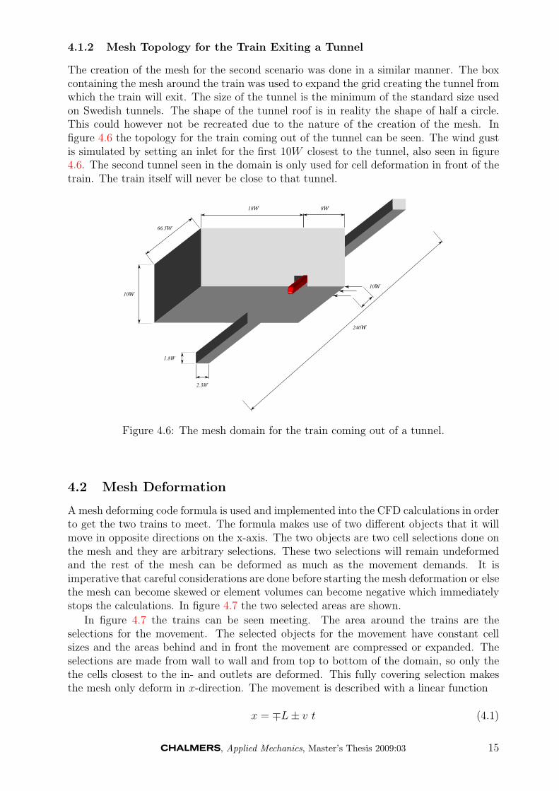
The creation of the mesh for the second scenario was done in a similar manner. The boxcontaining the mesh around the train was used to expand the grid creating the tunnel fromwhich the train will exit. The size of the tunnel is the minimum of the standard size usedon Swedish tunnels. The shape of the tunnel roof is in reality the shape of half a circle.This could however not be recreated due to the nature of the creation of the mesh. Infigure 4.6 the topology for the train coming out of the tunnel can be seen. The wind gustis simulated by setting an inlet for the first 10W closest to the tunnel, also seen in figure4.6. The second tunnel seen in the domain is only used for cell deformation in front of thetrain. The train itself will never be close to that tunnel.

10W

240W

2.3W

1.8W

10W

66.5W

18W 8W

Figure 4.6: The mesh domain for the train coming out of a tunnel.

4.2 Mesh Deformation

A mesh deforming code formula is used and implemented into the CFD calculations in orderto get the two trains to meet. The formula makes use of two different objects that it willmove in opposite directions on the x-axis. The two objects are two cell selections done onthe mesh and they are arbitrary selections. These two selections will remain undeformedand the rest of the mesh can be deformed as much as the movement demands. It isimperative that careful considerations are done before starting the mesh deformation or elsethe mesh can become skewed or element volumes can become negative which immediatelystops the calculations. In figure 4.7 the two selected areas are shown.

In figure 4.7 the trains can be seen meeting. The area around the trains are theselections for the movement. The selected objects for the movement have constant cellsizes and the areas behind and in front the movement are compressed or expanded. Theselections are made from wall to wall and from top to bottom of the domain, so only thethe cells closest to the in- and outlets are deformed. This fully covering selection makesthe mesh only deform in x-direction. The movement is described with a linear function

x = ∓L± v t (4.1)


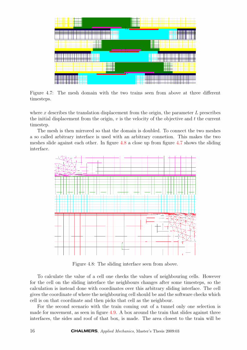
Figure 4.7: The mesh domain with the two trains seen from above at three differenttimesteps.

where x describes the translation displacement from the origin, the parameter L prescribesthe initial displacement from the origin, v is the velocity of the objective and t the currenttimestep.

The mesh is then mirrored so that the domain is doubled. To connect the two meshesa so called arbitrary interface is used with an arbitrary connetion. This makes the twomeshes slide against each other. In figure 4.8 a close up from figure 4.7 shows the slidinginterface.

Figure 4.8: The sliding interface seen from above.

To calculate the value of a cell one checks the values of neighbouring cells. Howeverfor the cell on the sliding interface the neighbours changes after some timesteps, so thecalculation is instead done with coordinates over this arbitrary sliding interface. The cellgives the coordinate of where the neighbouring cell should be and the software checks whichcell is on that coordinate and then picks that cell as the neighbour.

For the second scenario with the train coming out of a tunnel only one selection ismade for movement, as seen in figure 4.9. A box around the train that slides against threeinterfaces, the sides and roof of that box, is made. The area closest to the train will be


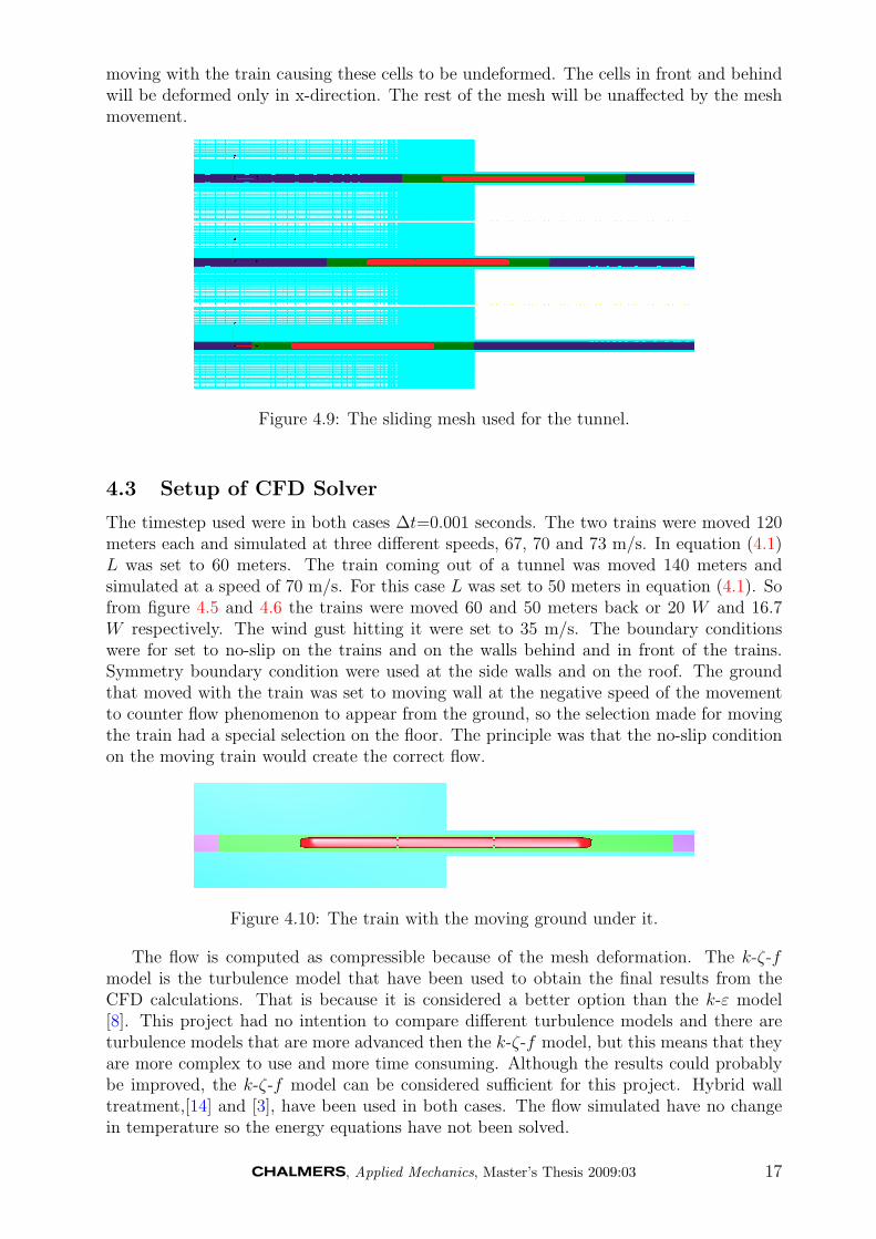
moving with the train causing these cells to be undeformed. The cells in front and behindwill be deformed only in x-direction. The rest of the mesh will be unaffected by the meshmovement.

Figure 4.9: The sliding mesh used for the tunnel.

4.3 Setup of CFD Solver

The timestep used were in both cases ∆t=0.001 seconds. The two trains were moved 120meters each and simulated at three different speeds, 67, 70 and 73 m/s. In equation (4.1)L was set to 60 meters. The train coming out of a tunnel was moved 140 meters andsimulated at a speed of 70 m/s. For this case L was set to 50 meters in equation (4.1). Sofrom figure 4.5 and 4.6 the trains were moved 60 and 50 meters back or 20 W and 16.7W respectively. The wind gust hitting it were set to 35 m/s. The boundary conditionswere for set to no-slip on the trains and on the walls behind and in front of the trains.Symmetry boundary condition were used at the side walls and on the roof. The groundthat moved with the train was set to moving wall at the negative speed of the movementto counter flow phenomenon to appear from the ground, so the selection made for movingthe train had a special selection on the floor. The principle was that the no-slip conditionon the moving train would create the correct flow.

Figure 4.10: The train with the moving ground under it.

The flow is computed as compressible because of the mesh deformation. The k-ζ-fmodel is the turbulence model that have been used to obtain the final results from theCFD calculations. That is because it is considered a better option than the k-ε model[8]. This project had no intention to compare different turbulence models and there areturbulence models that are more advanced then the k-ζ-f model, but this means that theyare more complex to use and more time consuming. Although the results could probablybe improved, the k-ζ-f model can be considered sufficient for this project. Hybrid walltreatment,[14] and [3], have been used in both cases. The flow simulated have no changein temperature so the energy equations have not been solved.


5 Method for Vibration Dynamic Simulations

In all dynamic simulations the coordinate system will have the x-axis in the longitudedirection, and the z-axis vertically downwards which is the same as the standard in flightdynamics. This means that the force and moments from the CFD simulations will have tochange signs for longitude, vertical, roll and yaw.

Table 5.1: Data for the train car.m Ix Iy Iz

35000[kg] 90× 103[kgm2] 1.8× 106[kgm2] 1.8× 106[kgm2]

The train will be expressed in a system of rigid bodies connected with linear springsand dampers, and for some simulations also a set of nonlinear connectors in the couplingbetween the cars. The actual train car is modeled as a single rigid body, connected to abogie frame. Its mass and mass moment of inertia is in table 5. The center of mass wasestimated to be at 1.22 meters from the top of the rail. The bogies are connected at ±9meters from the center of the car.

5.1 Bogie model

Figure 5.1: Reference photo of the bogie used in high speed trains.

The most important part of the system are the bogies. The bogie used in figure 5.1 hasbeen tested in speeds up towards 300 km/h within the Grona Taget research programme.Two mechanical models have been developed and both describe the same bogie. The firstmodel is more complicated, and is made to as accurately as possible describe the behaviourof the real bogie, and a second conventional bogie model for easier comparison with otherwork on train dynamics.

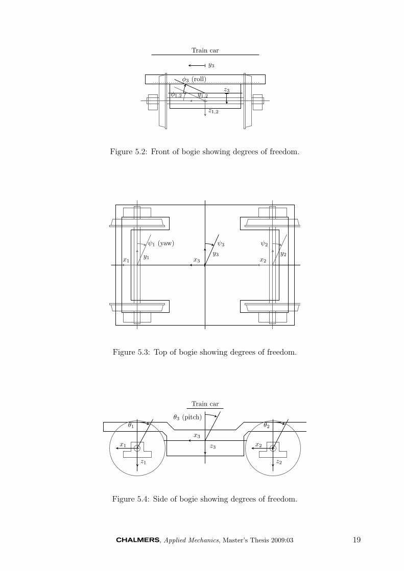
5.1.1 Degrees of Freedom

To simplify the contact behaviour the vertical displacement and the roll of the wheelsetsare locked in the simulations. The small vertical movement and roll which would occurwhen the wheelset moves laterally is very small, and can be assumed to be zero with littleeffect on the train dynamics. This also means that the wheelset will hold the train in place,i.e. the normal contact force can be negative, but at that point the instability of the trainwill be over any acceptable criteria.

The axle boxes are also neglected. The pitch on the wheelsets can rotate freely withrespect to the bogie, and the pitch of the axle box is not included in the degrees of freedom.For the displacement and yaw degrees of freedom the wheelset and axle box are merged.


y1,2

z1,2

φ1,2

y3

z3

φ3 (roll)

Train car

Figure 5.2: Front of bogie showing degrees of freedom.

y1x1

ψ1 (yaw)y2

x2

ψ2

y3x3

ψ3

Figure 5.3: Top of bogie showing degrees of freedom.

Train car

x3

z3

θ3 (pitch)

x1 x2

z1 z2

θ1 θ2

Figure 5.4: Side of bogie showing degrees of freedom.


5.1.2 Geometry of Bogie

Train car

h3

h1 h2

h4

h5

h6 h7

Figure 5.5: Front of bogie showing geometry.

d3

w3

d1d2

w1

x

yw4

w5w2

d4

Figure 5.6: Top of bogie showing geometry.

Train car

Figure 5.7: Side of bogie showing geomtry.

The bogie is simplified to two symmetry planes shown in figure 5.6.

5.1.3 Placement of Springs and Dampers

All springs and dampers are modeled with momentless joints, so a pair of horizontal springshave been added to each real vertical spring to simulate the horizontal stiffness and ro-tational stiffness of the bogie. The horizontal springs and dampers will be modeled with


Train car

Figure 5.8: Front of bogie showing springs and dampers.

1

2

4

5

13

4

Figure 5.9: Top of bogie showing springs and dampers.

Train car

632

5

Figure 5.10: Side of bogie showing springs and dampers.


zero relaxed length and is connected to the same point as the vertical spring at both ends,marked by red crosses for springs and blue crosses for dampers in figure 5.5 to figure 5.10.The model also assumes symmetry along both the x-axis and y-axis shown in figure 5.6.

The two vertical springs connecting the bogie to the train were changed to four verticalsprings (9 to 12 in figure 5.6) placed at the distance d3 in order to carry the momentbetween the bogie and train car. The spring stiffness and the distance d3 are to be adjustedaccording to the real springs vertical strength and bending strength.

Table 5.2: Spring and damper coefficients for the bogie. Numbers are shown in figure 5.9and 5.10.

Spring[kN/m] Damper[kNs/m]

1 2500 100/√

2

2 400 100/√

23 500 9004 90 155 90 156 90 -

Table 5.3: Geometry of the bogie. Numbers are shown in figure 5.6, 5.7 and 5.5.d[m] w[m] h[m]

1 1.3 0.9 0.22 0.1 1.1 0.253 0.1 0.9 -0.044 0.2 0.5 0.25 - 1.2 0.26 - - 07 - - 0.048 - - 0

The second bogie model implemented as a conventional bogie [10] with an additionalspring between bogie and train car was added.

Train car

h2

h1

h3

Figure 5.11: Front of conventional bogie showing springs.

For the conventional bogie model the placement is in figure 5.11, 5.12 and 5.13. Everyspring is in parallell with a damper which is not shown in the figures.


12

4

5

7

d1

w1

Figure 5.12: Top of conventional bogie showing springs.

Train car

6

3

Figure 5.13: Side of conventional bogie showing springs.

Table 5.4: Initial spring and damper coefficients for the conventional bogie. Numbers areshown in figure 5.12 and 5.13.

Spring Damper1 5000[kN/m] 0[kNs/m]

2 800[kN/m] 100/√

(2)[kNs/m]

3 1000[kN/m] 100/√

(2)[kNs/m]4 360[kN/m] 1800[kNs/m]5 180[kN/m] 7.5[kNs/m]6 180[kN/m] 4.629[kNs/m]7 292[kNm] 2178[kNsm]


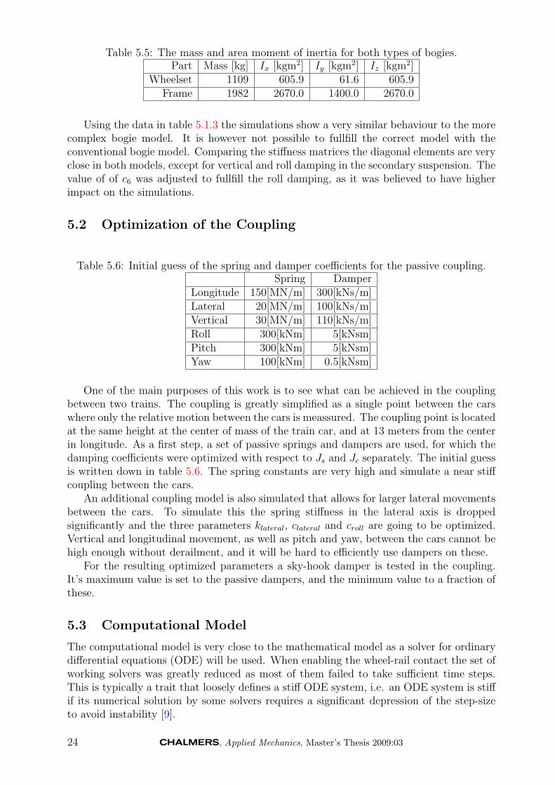
Table 5.5: The mass and area moment of inertia for both types of bogies.Part Mass [kg] Ix [kgm2] Iy [kgm2] Iz [kgm2]

Wheelset 1109 605.9 61.6 605.9Frame 1982 2670.0 1400.0 2670.0

Using the data in table 5.1.3 the simulations show a very similar behaviour to the morecomplex bogie model. It is however not possible to fullfill the correct model with theconventional bogie model. Comparing the stiffness matrices the diagonal elements are veryclose in both models, except for vertical and roll damping in the secondary suspension. Thevalue of of c6 was adjusted to fullfill the roll damping, as it was believed to have higherimpact on the simulations.

5.2 Optimization of the Coupling

Table 5.6: Initial guess of the spring and damper coefficients for the passive coupling.Spring Damper

Longitude 150[MN/m] 300[kNs/m]Lateral 20[MN/m] 100[kNs/m]Vertical 30[MN/m] 110[kNs/m]Roll 300[kNm] 5[kNsm]Pitch 300[kNm] 5[kNsm]Yaw 100[kNm] 0.5[kNsm]

One of the main purposes of this work is to see what can be achieved in the couplingbetween two trains. The coupling is greatly simplified as a single point between the carswhere only the relative motion between the cars is meassured. The coupling point is locatedat the same height at the center of mass of the train car, and at 13 meters from the centerin longitude. As a first step, a set of passive springs and dampers are used, for which thedamping coefficients were optimized with respect to Js and Jc separately. The initial guessis written down in table 5.6. The spring constants are very high and simulate a near stiffcoupling between the cars.

An additional coupling model is also simulated that allows for larger lateral movementsbetween the cars. To simulate this the spring stiffness in the lateral axis is droppedsignificantly and the three parameters klateral, clateral and croll are going to be optimized.Vertical and longitudinal movement, as well as pitch and yaw, between the cars cannot behigh enough without derailment, and it will be hard to efficiently use dampers on these.

For the resulting optimized parameters a sky-hook damper is tested in the coupling.It’s maximum value is set to the passive dampers, and the minimum value to a fraction ofthese.

5.3 Computational Model

The computational model is very close to the mathematical model as a solver for ordinarydifferential equations (ODE) will be used. When enabling the wheel-rail contact the set ofworking solvers was greatly reduced as most of them failed to take sufficient time steps.This is typically a trait that loosely defines a stiff ODE system, i.e. an ODE system is stiffif its numerical solution by some solvers requires a significant depression of the step-sizeto avoid instability [9].


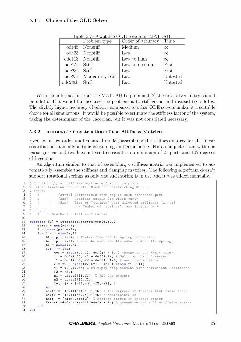
5.3.1 Choice of the ODE Solver

Table 5.7: Available ODE solvers in MATLAB.Problem type Order of accuracy Time

ode45 Nonstiff Medium ∞ode23 Nonstiff Low ∞

ode113 Nonstiff Low to high ∞ode15s Stiff Low to medium Fastode23s Stiff Low Fastode23t Moderately Stiff Low Untested

ode23tb Stiff Low Untested

With the information from the MATLAB help manual [2] the first solver to try shouldbe ode45. If it woudl fail because the problem is to stiff go on and instead try ode15s.The slightly higher accuracy of ode15s compared to other ODE solvers makes it a suitablechoice for all simulations. It would be possible to estimate the stiffness factor of the system,taking the determinant of the Jacobian, but it was not considered necessary.

5.3.2 Automatic Construction of the Stiffness Matrices

Even for a low order mathematical model, assembling the stiffness matrix for the linearcontribution manually is time consuming and error-prone. For a complete train with onepassenger car and two locomotives this results in a minimum of 21 parts and 102 degreesof freedome.

An algorithm similar to that of assembling a stiffness matrix was implemented to au-tomatically assemble the stiffness and damping matrices. The following algorithm doesn’tsupport rotational springs as only one such spring is in use and it was added manually.

1 % function [X] = StiffnessConstructor(pxtot ,xconp ,vx)

2 % Helper function for models. Used for constructing K or C.

3 % Input:

4 % x : [3xnx2] Coordinates from cog on each connected part

5 % c : [2xn] Coupling matrix (to which part)

6 % v : [3xn] List of "springs" with directed stiffness [x,y,z]

7 % n = Number of "springs", any integer >= 0

8 % Output:

9 % X : [6* nx6*n] "Stiffness" matrix

1011 function [X] = StiffnessConstructor(p,c,v)

12 parts = max(c(:));

13 X = zeros(parts *6);

14 for i = 1:size(v,2)

15 L1 = p(:,i,1); % Vector from COG to spring connection

16 L2 = p(:,i,2); % and the same for the other end of the spring

17 Xe = zeros (12);

18 for j = 1:12

19 dof = zeros (12 ,1); dof(j) = 1; % change in dof (unit size)

20 t1 = dof (1:3); t2 = dof (7:9); % Split up the dof -vector

21 r1 = dof (4:6); r2 = dof (10:12); % and into rotation

22 d = t2 + cross(r2,L2) - (t1 + cross(r1 ,L1));

23 f1 = v(:,i).*d; % Multiply displacement with directional stiffness

24 f2 = -f1;

25 m1 = crossf(L1,f1); % And the moments

26 m2 = crossf(L2,f2);

27 Xe(:,j) = [-f1;-m1;-f2;-m2]; %

28 end

29 edof1 = (1:6) +(c(1,i) -1)*6; % The degrees of freedom that these loads

30 edof2 = (1:6) +(c(2,i) -1)*6; % corresponds to.

31 edof = [edof1 ,edof2]; % Element degree of freedom vector

32 X(edof ,edof) = X(edof ,edof) + Xe; % Assembles the full stiffness matrix

33 end

34 end


The algorithm is suitable for any multibody system with springs or dampers and wasmainly used to calculate the stiffness contribution from the bogies.

6 Results from Aerodynamic Simulations

The primary objective of the results from the aerodynamic simulations is to be used in thedynamic calculations. The results from the scenarios differs greatly from each other. It isinteresting to study where the different forces come from and why they behave like theydo.

6.1 Two Trains Meeting at High Speed

In figure 6.1 one can see the upcoming impact from the two trains passing each other athigh speed. The distribution of the pressure can be seen on the train bodies as well asvortices created from the tail of the train.

Figure 6.1: The meeting of two trains.

Figure 6.2: The relative pressure acting on the train.

The relative pressure on the train is seen in figure 6.2. This profile is taken from theleft train in figure 6.1. This is the characteristic profile of where the pressure is high and


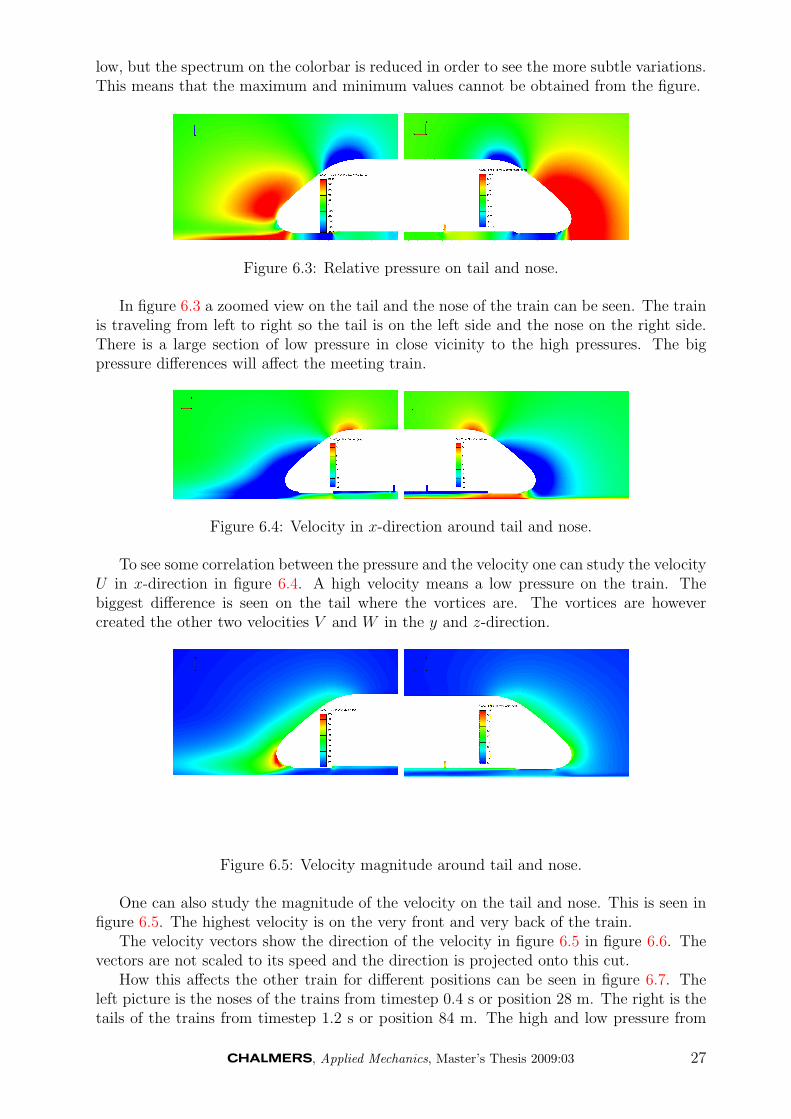
low, but the spectrum on the colorbar is reduced in order to see the more subtle variations.This means that the maximum and minimum values cannot be obtained from the figure.

Figure 6.3: Relative pressure on tail and nose.

In figure 6.3 a zoomed view on the tail and the nose of the train can be seen. The trainis traveling from left to right so the tail is on the left side and the nose on the right side.There is a large section of low pressure in close vicinity to the high pressures. The bigpressure differences will affect the meeting train.

Figure 6.4: Velocity in x-direction around tail and nose.

To see some correlation between the pressure and the velocity one can study the velocityU in x-direction in figure 6.4. A high velocity means a low pressure on the train. Thebiggest difference is seen on the tail where the vortices are. The vortices are howevercreated the other two velocities V and W in the y and z-direction.

Figure 6.5: Velocity magnitude around tail and nose.

One can also study the magnitude of the velocity on the tail and nose. This is seen infigure 6.5. The highest velocity is on the very front and very back of the train.

The velocity vectors show the direction of the velocity in figure 6.5 in figure 6.6. Thevectors are not scaled to its speed and the direction is projected onto this cut.

How this affects the other train for different positions can be seen in figure 6.7. Theleft picture is the noses of the trains from timestep 0.4 s or position 28 m. The right is thetails of the trains from timestep 1.2 s or position 84 m. The high and low pressure from


Figure 6.6: Velocity vectors around tail and nose.

Figure 6.7: High and low pressure on the train at different positions seen from above. Theupper train is moving from left to right.

the nose of the trains is having a great influence on the meeting train. Same thing goesfor the low and high pressure from the tail of the trains.

Figure 6.8: The relative pressure around the train.

The alignment of the trains are what gives one of the most interesting effects. The high


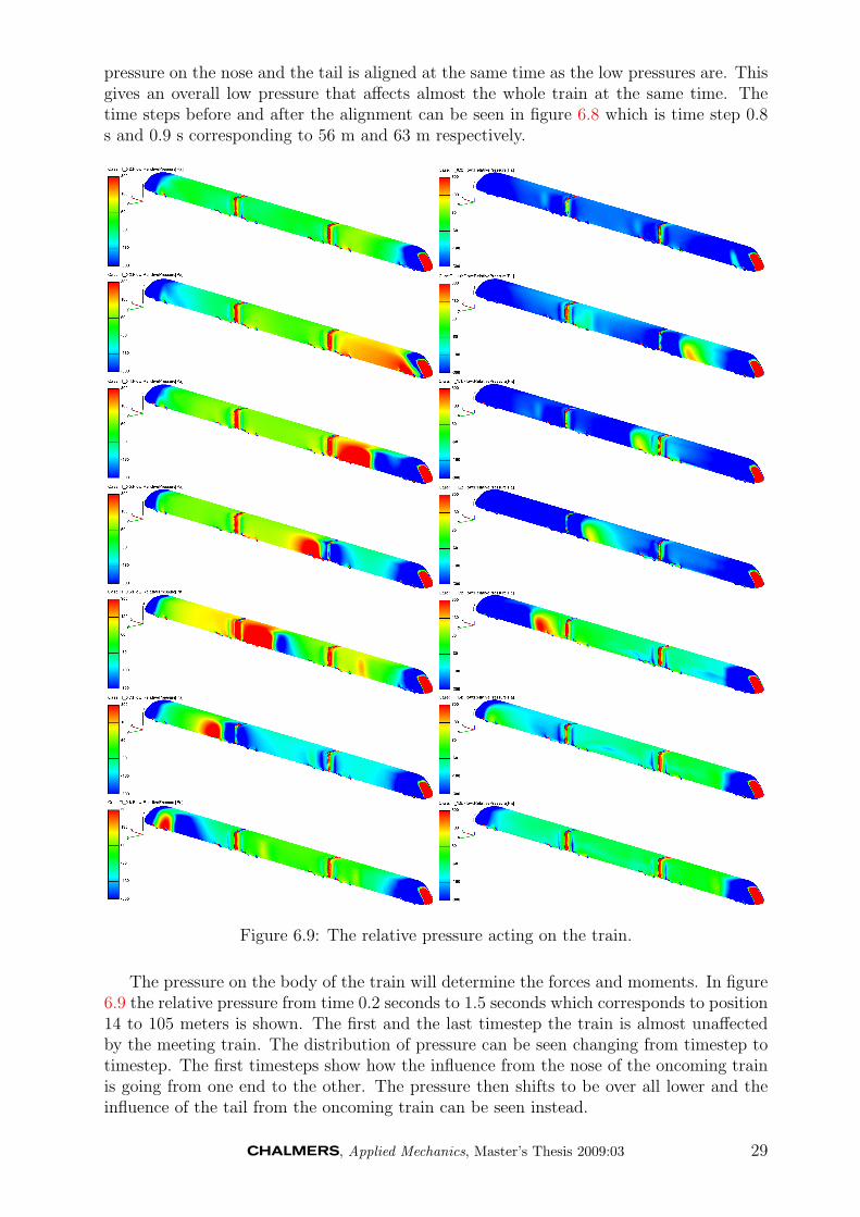
pressure on the nose and the tail is aligned at the same time as the low pressures are. Thisgives an overall low pressure that affects almost the whole train at the same time. Thetime steps before and after the alignment can be seen in figure 6.8 which is time step 0.8s and 0.9 s corresponding to 56 m and 63 m respectively.

Figure 6.9: The relative pressure acting on the train.

The pressure on the body of the train will determine the forces and moments. In figure6.9 the relative pressure from time 0.2 seconds to 1.5 seconds which corresponds to position14 to 105 meters is shown. The first and the last timestep the train is almost unaffectedby the meeting train. The distribution of pressure can be seen changing from timestep totimestep. The first timesteps show how the influence from the nose of the oncoming trainis going from one end to the other. The pressure then shifts to be over all lower and theinfluence of the tail from the oncoming train can be seen instead.


0 20 40 60 80 100

−1

0

1

x 104 Front

1

Forc

e[N

]

1

FD

1

FS

1

FL

1

0 20 40 60 80 100

−1

0

1

x 105

Position [m]

1

Mom

ent

[Nm

]

1

MR

1

MP

1

MY

1

0 20 40 60 80 100−1

−0.5

0

0.5

1

1.5

x 104 Rear

1

Forc

e[N

]

1

FD

1

FS

1

FL

1

0 20 40 60 80 100−1

−0.5

0

0.5

1

1.5x 105

Position [m]

1

Mom

ent

[Nm

]

1

MR

1

MP

1

MY

1

0 20 40 60 80 100

−5000

0

5000

10000Mid

1

Forc

e[N

]

1

FD

1

FS

1

FL

1

0 20 40 60 80 100

−5

0

5

x 104

Position [m]

1

Mom

ent

[Nm

]

1

MR

1

MP

1

MY

1

Figure 6.10: The forces and moments acting on the train cars.

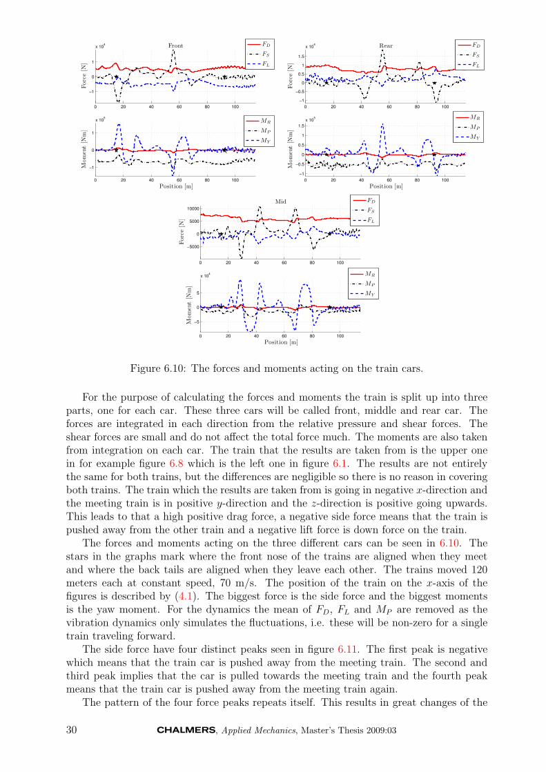
For the purpose of calculating the forces and moments the train is split up into threeparts, one for each car. These three cars will be called front, middle and rear car. Theforces are integrated in each direction from the relative pressure and shear forces. Theshear forces are small and do not affect the total force much. The moments are also takenfrom integration on each car. The train that the results are taken from is the upper onein for example figure 6.8 which is the left one in figure 6.1. The results are not entirelythe same for both trains, but the differences are negligible so there is no reason in coveringboth trains. The train which the results are taken from is going in negative x-direction andthe meeting train is in positive y-direction and the z-direction is positive going upwards.This leads to that a high positive drag force, a negative side force means that the train ispushed away from the other train and a negative lift force is down force on the train.

The forces and moments acting on the three different cars can be seen in 6.10. Thestars in the graphs mark where the front nose of the trains are aligned when they meetand where the back tails are aligned when they leave each other. The trains moved 120meters each at constant speed, 70 m/s. The position of the train on the x-axis of thefigures is described by (4.1). The biggest force is the side force and the biggest momentsis the yaw moment. For the dynamics the mean of FD, FL and MP are removed as thevibration dynamics only simulates the fluctuations, i.e. these will be non-zero for a singletrain traveling forward.

The side force have four distinct peaks seen in figure 6.11. The first peak is negativewhich means that the train car is pushed away from the meeting train. The second andthird peak implies that the car is pulled towards the meeting train and the fourth peakmeans that the train car is pushed away from the meeting train again.

The pattern of the four force peaks repeats itself. This results in great changes of the


yaw moment. Note that the first two side force peaks result in negative yaw moment peaksand the last two side force peaks result in positive yaw moment peaks. The transition oftwo force changing sign give the moment of opposite signs of the peaks. The roll momentof the cars are very much dependent on the position of the center of gravity of the cars.This is not known so an estimation is made.

0 20 40 60 80 100

−1.5

−1

−0.5

0

0.5

1

1.5

x 104

Position [m]

1

Forc

e[N

]

1

Front

1

Mid

1

Rear

1

Figure 6.11: Side force on the different cars meeting another train at 140 m/s.

The side force on the different cars can be seen in figure 6.11. One can observe howthe forces from the meeting of the other train is going from one car to the next. The forcetravels with double the speed of one train, i.e their relative speed, 140 m/s.

0 20 40 60 80 100

−8000

−6000

−4000

−2000

0

2000

4000

6000

8000

10000

12000

Position [m]

1

Forc

e[N

]

1

u67

1

u70

1

u73

1

Figure 6.12: Side force on the middle car at speed 67, 70 and 73 m/s.


The forces on the middle car at three different velocities can be seen in figure 6.12. Thereis not much difference between them in magnitude. In general the higher the velocity thebigger the force. However for the the first two peaks the highest amplitude is from the 70m/s case. And the last peak the 67 m/s case is higher then the 70 m/s one. The differencesbetween the speeds are not big, but at these small changes the forces already differ a bitin behaviour.

0 20 40 60 80 1000

0.20.40.60.8

CD

1

0 20 40 60 80 100−0.5

0

0.5

1

CS

1

0 20 40 60 80 100−0.4

−0.2

0

Position [m]

1

CL

1

0 20 40 60 80 100−0.3−0.2−0.1

00.1

CRM

1

0 20 40 60 80 100−2

−1

0

CPM

1

0 20 40 60 80 100−1

0

1

2

Position [m]

1

CYM

1

Figure 6.13: The force coefficients on the train from meeting a train at 140 m/s.

The forces and moments on the whole train traveling at 70 m/s can also be studiedand seen in figure 6.13. The force coefficients are on the left and the moment coefficientsare on the right. There is a distinct force amplitude when the trains are aligned with eachother. This is when the forces from low pressures from the front car and rear car collapseswhich makes the two trains being pulled towards one another.

The coefficients for the different velocities can be seen in table 6.1.

Table 6.1: Coefficients from the meeting trains scenario.Mean CD CS CL CRM CPM CYMu67 0.66360 0.05968 -0.09752 -0.02177 -1.52177 0.11707u70 0.65961 0.05966 -0.09954 -0.02059 -1.52515 0.09030u73 0.65758 0.05823 -0.09418 -0.02043 -1.51897 0.09519

Variance CD CS CL CRM CPM CYMu67 0.00657 0.06634 0.00649 0.00461 0.04679 0.48449u70 0.00650 0.07291 0.00675 0.00514 0.04103 0.49875u73 0.00634 0.07555 0.00668 0.00541 0.04170 0.50117

6.2 Train Exiting a Tunnel under Influence of a Wind Gust

Figure 6.14 show the train coming out of the tunnel at time step 0.6 s or position 42 m.The train is traveling in 70 m/s and the wind have a initial speed of 35 m/s. The trainstarts inside the tunnel and goes all the way out and past the wind gust.

In figure 6.15 the iso surfaces of low pressure are shown from the same position as seenin figure 6.14. The surfaces are colored by velocity W ,i.e in z-direction. The red surfacesare wind going upwards and the blue are wind going downwards. The effect this has onthe pressure of the train can be seen in the right picture where the relative pressure on thetrain body is shown.


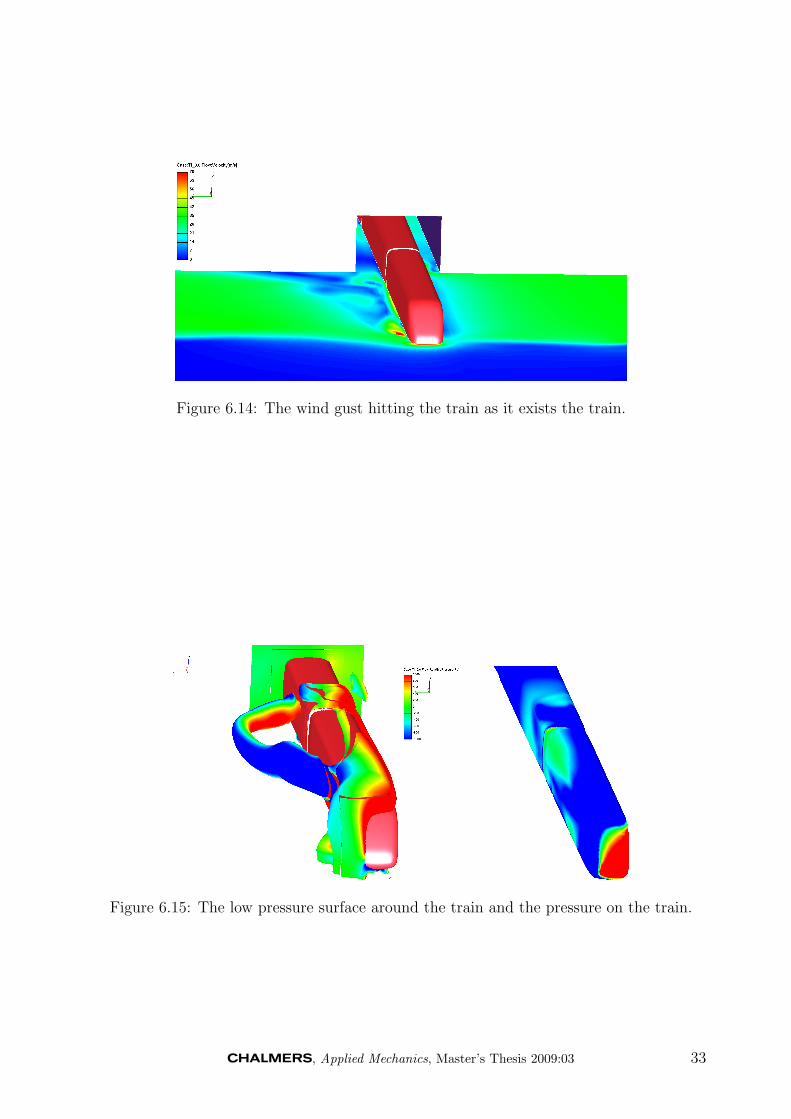
Figure 6.14: The wind gust hitting the train as it exists the train.

Figure 6.15: The low pressure surface around the train and the pressure on the train.


For the full scenario of pressure on the train one can study the time steps shown infigure 6.16. Note how the very low pressure on the top of the train travels as the trainis exiting. This will cause a large lift force. Note also how the high pressure on the sidetravels from car to car. The magnitude of this pressure is however going down as the traintravel, causing the side force to go down as well.

Figure 6.16: The relative pressure acting on the train during exit of tunnel.


0 20 40 60 80 100 1200

5

10

x 104 Front

1

Forc

e[N

]

1

FD

1

FS

1

FL

1

0 20 40 60 80 100 120−8

−6

−4

−2

0

2

x 105

Position [m]

1

Mom

ent

[Nm

]

1

MR

1

MP

1

MY

1

0 20 40 60 80 100 120−5

0

5

10

15x 104 Rear

1

Forc

e[N

]

1

FD

1

FS

1

FL

1

0 20 40 60 80 100 120

−4

−2

0

2

x 105

Position [m]

1

Mom

ent

[Nm

]

1

MR

1

MP

1

MY

1

0 20 40 60 80 100 1200

5

10

x 104 Mid

1

Forc

e[N

]

1

FD

1

FS

1

FL

1

0 20 40 60 80 100 120

−4

−2

0

2

4x 105

Position [m]

1

Mom

ent

[Nm

]

1

MR

1

MP

1

MY

1

Figure 6.17: The forces and moments acting on the train cars.

The scenario was performed with the train traveling at 70 m/s and an inlet wind of 35m/s at the first 30 m (10W ) from the tunnel exit. This is meant to simulate a strong windgust influencing the train when exiting the tunnel.

In figure 6.17 the forces and moments acting on the different cars can be seen. Thestars mark when the nose of the train exit the tunnel and when the rear tail of the trainexit the tunnel. The lift force is the greatest force acting on the train and can be seenwander from one car to the next during the exit of the tunnel.

0 20 40 60 80 100 1200

1

2

CD

1

0 20 40 60 80 100 120

0

2

4

CS

1

0 20 40 60 80 100 1200

2

4

6

Position [m]

1

CL

1

0 20 40 60 80 100 120

−1

−0.5

0

CRM

1

0 20 40 60 80 100 120−6−4−2

02

CPM

1

0 20 40 60 80 100 120−10

−5

0

5

Position [m]

1

CYM

1

Figure 6.18: The force coefficients on the train from meeting a train at 140 m/s.

The coefficients were calculated for the whole train as in (2.18-2.19) and is seen in figure6.18.


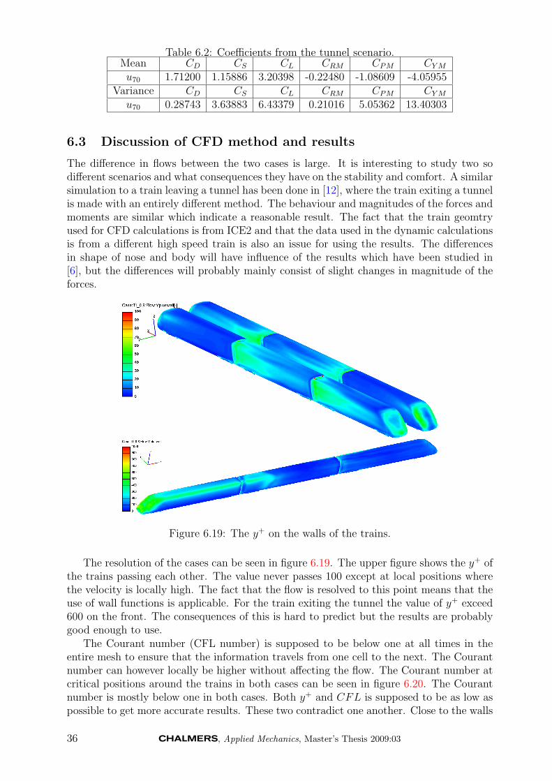
Table 6.2: Coefficients from the tunnel scenario.Mean CD CS CL CRM CPM CYMu70 1.71200 1.15886 3.20398 -0.22480 -1.08609 -4.05955

Variance CD CS CL CRM CPM CYMu70 0.28743 3.63883 6.43379 0.21016 5.05362 13.40303

6.3 Discussion of CFD method and results

The difference in flows between the two cases is large. It is interesting to study two sodifferent scenarios and what consequences they have on the stability and comfort. A similarsimulation to a train leaving a tunnel has been done in [12], where the train exiting a tunnelis made with an entirely different method. The behaviour and magnitudes of the forces andmoments are similar which indicate a reasonable result. The fact that the train geomtryused for CFD calculations is from ICE2 and that the data used in the dynamic calculationsis from a different high speed train is also an issue for using the results. The differencesin shape of nose and body will have influence of the results which have been studied in[6], but the differences will probably mainly consist of slight changes in magnitude of theforces.

Figure 6.19: The y+ on the walls of the trains.

The resolution of the cases can be seen in figure 6.19. The upper figure shows the y+ ofthe trains passing each other. The value never passes 100 except at local positions wherethe velocity is locally high. The fact that the flow is resolved to this point means that theuse of wall functions is applicable. For the train exiting the tunnel the value of y+ exceed600 on the front. The consequences of this is hard to predict but the results are probablygood enough to use.

The Courant number (CFL number) is supposed to be below one at all times in theentire mesh to ensure that the information travels from one cell to the next. The Courantnumber can however locally be higher without affecting the flow. The Courant number atcritical positions around the trains in both cases can be seen in figure 6.20. The Courantnumber is mostly below one in both cases. Both y+ and CFL is supposed to be as low aspossible to get more accurate results. These two contradict one another. Close to the walls


Figure 6.20: The Courant number on the walls around the trains.

where y+ is calculated the Courant number is calculated for the same height, i.e. y = h in(2.20) and (2.23). So having small cells to resolve the flow also means that the time stephas to be lowered.

7 Results from Vibration Dynamic Simulations

Throughout all results all the cost functions should be minized, i.e. a lower Jc, Js,1 andJs,2 is better, where they meassure comfort and two stability measurements respectively.In the scenario with meeting trains, the flange never touches the rail, so Js,1 is zero for allsimulations.

60 62 64 66 68 70 72 74 76 78 800.8

0.85

0.9

0.95

1

1.05

1.1

1.15

1.2

1.25

V [m/s]

1

Meeting trains

1

Jc

1

Js,1

1

Js,2

1

60 62 64 66 68 70 72 74 76 78 800.75

0.8

0.85

0.9

0.95

1

1.05

1.1

1.15

1.2

1.25

V [m/s]

1

Tunnel and side wind

1

Jc

1

Js,1

1

Js,2

1

Figure 7.1: Comfort and stability measurements over speed with the initial spring anddamper coefficients for a passive coupling.


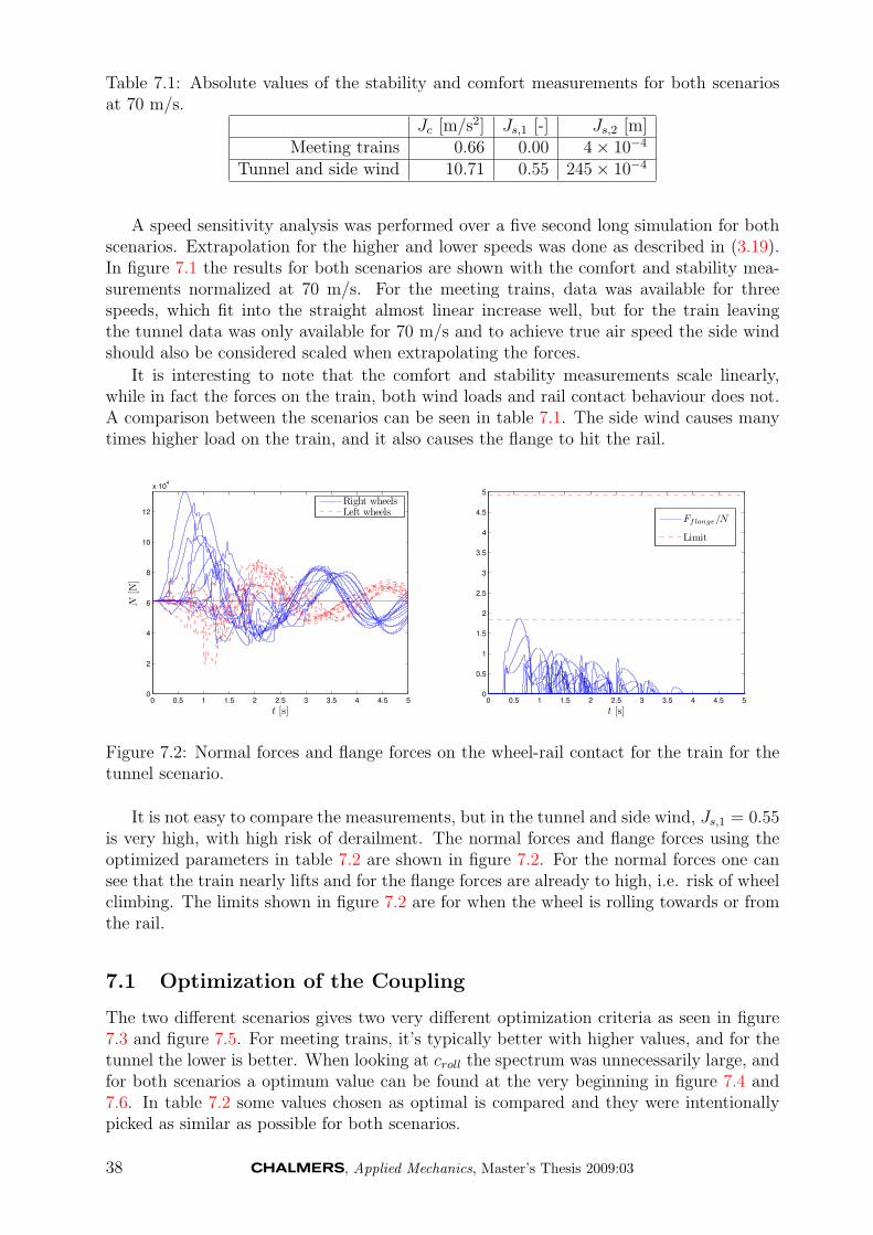
Table 7.1: Absolute values of the stability and comfort measurements for both scenariosat 70 m/s.

Jc [m/s2] Js,1 [-] Js,2 [m]Meeting trains 0.66 0.00 4× 10−4

Tunnel and side wind 10.71 0.55 245× 10−4

A speed sensitivity analysis was performed over a five second long simulation for bothscenarios. Extrapolation for the higher and lower speeds was done as described in (3.19).In figure 7.1 the results for both scenarios are shown with the comfort and stability mea-surements normalized at 70 m/s. For the meeting trains, data was available for threespeeds, which fit into the straight almost linear increase well, but for the train leavingthe tunnel data was only available for 70 m/s and to achieve true air speed the side windshould also be considered scaled when extrapolating the forces.

It is interesting to note that the comfort and stability measurements scale linearly,while in fact the forces on the train, both wind loads and rail contact behaviour does not.A comparison between the scenarios can be seen in table 7.1. The side wind causes manytimes higher load on the train, and it also causes the flange to hit the rail.

0 0.5 1 1.5 2 2.5 3 3.5 4 4.5 50

2

4

6

8

10

12

x 104

t [s]

1

N[N

]

1

Right wheels

1

Left wheels

1

0 0.5 1 1.5 2 2.5 3 3.5 4 4.5 50

0.5

1

1.5

2

2.5

3

3.5

4

4.5

5

t [s]

1

Fflange/N

1

Limit

1

Figure 7.2: Normal forces and flange forces on the wheel-rail contact for the train for thetunnel scenario.

It is not easy to compare the measurements, but in the tunnel and side wind, Js,1 = 0.55is very high, with high risk of derailment. The normal forces and flange forces using theoptimized parameters in table 7.2 are shown in figure 7.2. For the normal forces one cansee that the train nearly lifts and for the flange forces are already to high, i.e. risk of wheelclimbing. The limits shown in figure 7.2 are for when the wheel is rolling towards or fromthe rail.

7.1 Optimization of the Coupling

The two different scenarios gives two very different optimization criteria as seen in figure7.3 and figure 7.5. For meeting trains, it’s typically better with higher values, and for thetunnel the lower is better. When looking at croll the spectrum was unnecessarily large, andfor both scenarios a optimum value can be found at the very beginning in figure 7.4 and7.6. In table 7.2 some values chosen as optimal is compared and they were intentionallypicked as similar as possible for both scenarios.


klateral [N/m]

1

c lateral

[Ns/

m]

1

Jc

1

0.2 0.4 0.6 0.8 1 1.2 1.4 1.6 1.8 2x 107

1

2

3

4

5

6

7

8

9

10x 105

0.94

0.96

0.98

1

1.02

1.04

1.06

1.08

klateral [N/m]

1

c lateral

[Ns/

m]

1

Js,2

1

0.2 0.4 0.6 0.8 1 1.2 1.4 1.6 1.8 2x 107

1

2

3

4

5

6

7

8

9

10x 105

0.99

0.995

1

1.005

1.01

1.015

1.02

1.025

1.03

1.035

Figure 7.3: Optimization of the lateral spring and damper for meeting trains.

104 105 1060.9

0.92

0.94

0.96

0.98

1

1.02

1.04

1.06

1.08

croll [Nsm]

1

Meeting trains

1

Jc

1

Js,1

1

Js,2

1

Figure 7.4: Optimization of the roll damper for meeting trains.

Table 7.2: Comparison of the optimized values.Initial Meeting trains Tunnel and side win

klateral [kN/m] 2×104 50 50clateral [kNs/m] 100 700 100croll [kNsm] 5 20 20Relative change of Jc -7.82% -7.18%Relative change of Js,1 -4.58%Relative change of Js,2 -0.55% -8.88%Effect in speed -3 to -4[m/s] -3 to -5[m/s]


klateral [N/m]

1

c lateral

[Ns/

m]

1

Jc

1

0.2 0.4 0.6 0.8 1 1.2 1.4 1.6 1.8 2x 107

1

2

3

4

5

6

7

8

9

10x 105

0.98

0.982

0.984

0.986

0.988

0.99

0.992

0.994

0.996

0.998

klateral [N/m]

1

c lateral

[Ns/

m]

1

Js,1

1

0.2 0.4 0.6 0.8 1 1.2 1.4 1.6 1.8 2x 107

1

2

3

4

5

6

7

8

9

10x 105

0.96

0.965

0.97

0.975

0.98

0.985

0.99

0.995

klateral [N/m]

1

c lateral

[Ns/

m]

1

Js,2

1

0.2 0.4 0.6 0.8 1 1.2 1.4 1.6 1.8 2x 107

1

2

3

4

5

6

7

8

9

10x 105

0.955

0.96

0.965

0.97

0.975

0.98

0.985

0.99

0.995

Figure 7.5: Optimization of the lateral spring and damper for tunnel and side wind.

105 1060.88

0.9

0.92

0.94

0.96

0.98

1

1.02

1.04

1.06

croll [Nsm]

1


1

Jc

1

Js,1

1

Js,2

1

Figure 7.6: Optimization of the roll damper for tunnel and side wind.


0 1 2 3 4 5−6

−4

−2

0

2

4

6

8x 10−3

t [s]

1

Dis

plac

emen

tof

car

[m]

1

0 1 2 3 4 5−10

−8

−6

−4

−2

0

2

4

6

8x 10−3

t [s]

1

Rot

atio

nof

car

[-]

1

x

1

y

1

z

1

x optimized

1

y optimized

1

z optimized

1

0 1 2 3 4 5−6

−4

−2

0

2

4

6

8x 10−4

t [s]

1

Dis

plac

emen

tof

whe

else

t[m

]

1

0 1 2 3 4 5−1.5

−1

−0.5

0

0.5

1

1.5x 10−4

t [s]

1

Rot

atio

nof

whe

else

t[-

]

1

y

1

y optimized

1

z

1

z optimized

1

Figure 7.7: The trains displacement for the meeting trains.

0 1 2 3 4 5−0.2

−0.15

−0.1

−0.05

0

0.05

0.1

0.15

0.2

t [s]

1

Dis

plac

emen

tof

car

[m]

1

0 1 2 3 4 5−0.2

−0.15

−0.1

−0.05

0

0.05

0.1

0.15

t [s]

1

Rot

atio

nof

car

[-]

1

x

1

y

1

z

1

x optimized

1

y optimized

1

z optimized

1

0 1 2 3 4 5−0.015

−0.01

−0.005

0

0.005

0.01

0.015

0.02

t [s]

1

Dis

plac

emen

tof

whe

else

t[m

]

1

0 1 2 3 4 5−0.02

−0.015

−0.01

−0.005

0

0.005

0.01

t [s]

1

Rot

atio

nof

whe

else

t[-

]

1

y

1

y optimized

1

z

1

z optimized

1

Figure 7.8: The trains displacement for the tunnel and side wind.

Figure 7.7 and 7.8 shows how the middle train car and the front wheelset on the middlecar responds in each respective scenario.


7.2 Coupling Sky-hook

0 0.2 0.4 0.6 0.8 10.998

0.999

1

1.001

1.002

1.003

1.004

1.005

f

1


1

Jc

1

Js,1

1

Js,2

1

0 0.1 0.2 0.3 0.4 0.5 0.6 0.7 0.8 0.9 10.995

1

1.005

1.01

1.015

1.02

1.025

1.03

1.035

f

1

Meeting trains

1

Jc

1

Js,1

1

Js,2

1

Figure 7.9: Sky-Hook for varying fractions.

0 0.2 0.4 0.6 0.8 11

1.01

1.02

1.03

1.04

1.05

1.06

1.07

1.08

f

1


1

Jc

1

Js,1

1

Js,2

1

0 0.2 0.4 0.6 0.8 10.99

1

1.01

1.02

1.03

1.04

1.05

1.06

1.07

f

1

Meeting trains

1

Jc

1

Js,1

1

Js,2

1

Figure 7.10: Ground-Hook for varying fractions.

By sky-hook in these simulations the sky is referred to as the locomotives, and themiddle car the ground. If vsky∆v > 0 then just a fraction, f , of the damping coefficient isused, i.e. cy,min = fcy and croll,min = fcroll. For the sky-hook on the meeting trains theODE solver had problems, thus the values are missing.

8 Conclusions

Only a few simplifications were done on the model as a whole which are described andmotivated in the theory for this report. The implementation in MATLAB used high levelmathematics and automated construction to minimize the amount of manual work. Thecontact model was built upon established techniques for contact, creep and forces. Thecomponents of the system have been tested individual and the dynamic simulations arevery trustworthy.

The scenario with the meeting trains will only cause slight vibrations for the passengers,while the tunnel and side wind has a major impact on the stability of the train. Forthe side wind at 35 m/s the train would experience to much movement, and at theseweather conditions (12 on the Beaufort scale) the train cannot go at full speed due to


safety concerns. Such wind can make large objects airborn and these conditions occur afew times a year around Europe.

One of the most interesting results is how very linearly the stability and comfort mea-surements scale towards the true air speed. The CFD simulations only cover a spectrumbetween 67 to 73 m/s in the meeting trains scenario, and only for 70m/s for the tunnel, butthe loads on the train behaves very similarly between 67 and 73m/s making it reasonable toscale using constant drag and lift coefficients. Even if the flow starts to behave differentlywhen nearing 60 and 80 m/s, the speed analysis still show that the comfort and stabilitystill change linearly for a quadratically changing wind load and highly nonlinear reactionforces from the wheel contact.

The swaying movement of the train car in both scenarios can most likely be dampedefficiently by the secondary suspension and most research on train dynamics focus onjust the bogie. This work shows that there is also a noteable room for improvementsin the coupling between the car bodies. While the initial parameters for the couplingwere not accurately calibrated after an actual high speed train, the simulations show thatcarefully adjusting the coupling is important and can make a difference that equals theeffect of lowering the speed around 3 m/s ≈ 10 km/h. The initial coupling parameters onlymodel a simple, stiff connection with some small internal damping and the real couplingmight already have better or worse behaviour. In particular the effects from changingthe roll damper are very strong for smaller values, making it unreasonable to believe thata optimized coupling is already in place, unless a similar analysis have been performed.Lowering the lateral stiffness by designing a momentless joint in the coupling might be agood idea, but more scenarios needs to be studied.

9 Recommendations

For further work we recommend the following:

• Improve mesh for movement. Some information is lost when the mesh is moved farfrom the initial position. The mesh quality could also be improved, the automaticmesh generator does not create a perfect mesh.

• It is difficult to use a moving mesh. Much control is lost. They are time consumingand when a calculation is started it is difficult to alter the settings.

• More velocity tests is needed. The velocities of the meeting trains should be done atseveral more velocities as well as the velocity of the train and the wind speed for thetunnel scenario. More is always good for use in the dynamic calculations.

• Cases with side wind velocity should be lowered. The 35 m/s currently used is aworst case scenario. To improve dynamic calculations and optimization of trainslower wind velocities should be used.

• Look at PID regulators in the coupling.

• Compare the performance of active damping in the secondary suspension to thecoupling.

• Compare stability and comfort measurements with non wind related scenarios suchas curves.

• The other springs and dampers could also be put under optimization, especially theroll spring.


References

[1] Fire v2008 cfd solver manual, 2008.

[2] Matlab manual for ode solvers. http://www.mathworks.com/access/helpdesk/

help/techdoc/ref/ode45.html, 2008.

[3] Branislav Basara. An eddy viscosity transport model based on elliptic relaxationapproach. AIAA J., 44:1686–1690, 2006.

[4] Bengt Sundstrom et al. Handbok och formelsamling i Hallfasthetslara. Fingraf AB,Sodertalje, Sweden, 2005.

[5] Bo Jonsson et al. Hoga hastigheter i SJ persontrafik. SJ Centralforvaltning, Stockholm,Sweden, 1969.

[6] Erik Bjerklund et al. Design of High-Speed Trains for Cross-Wing Stability. ChalmersTekniska Hogskola, 2007.

[7] Evert Andersson et al. Rail Vehicle Dynamics. Universitetsservice AB, Stockholm,Sweden, 2007.

[8] Kemal Hanjalic et al. A robust near-wall elliptic-relaxation eddy-viscosity turbulencemodel for cfd. International Journal of Heat and Fluid Flow, 25:1047–1051, 2004.

[9] Arieh Iserles. A First Course in the Numerical Analysis of Differential Equations.Cambridge University Press, 2004.

[10] Carsten Nordstrøm Jensen and Hans True. Application of a wheel-rail contact modelto railway dynamics in small radius curved tracks. Nonlinear Dynamics, 13:117–129,1997.

[11] K.L. Johnson. Contact Mechanics. Cambridge University Press, 1985.

[12] Sinisa Krajnovic. Computer simulation of a train exiting a tunnel through a varyingcrosswind. International Journal of Railway, 3:99–105, 2008.

[13] Joao C. Pombo and Jorge A.C. Ambrosio. Application of a wheel-rail contact modelto railway dynamics in small radius curved tracks. Multibody Syst Dyn, 19:91–114,2008.

[14] M. Popovac and K. Hanjalic. Compound wall treatment for rans computation ofcomplex turbulent flows and heat transfer. Turbulence and Combustion, 78:177–202,2007.


http://www.mathworks.com/access/helpdesk/help/techdoc/ref/ode45.html

http://www.mathworks.com/access/helpdesk/help/techdoc/ref/ode45.html

stability of high speed train under aerodynamic...

Documents