stability of discrete integration algorithms for a real-time

Stability of Discrete Integration Algorithmsfor a Real-Time, Second-Order System

R. E. McFarland

NASA, Ames Research Center

October, 1997

Real-time implementations of damped, second-order systems are examined in terms ofstability of the discrete realizations. In this analysis the required double integration isseparated, because nonlinearities are assumed to accompany the outputs of each discreteintegration algorithm. For example, “anti-windup” limiters may be assumed in a controlsystem application, as shown in the Laplace representation given by Fig. 1.

ωn2

2ζωn

1s

1s

x s( ) ˙y s( ) y s( ) y s( )˙ , ˙y yB T y yB T,

Fig. 1 - Laplace Representation

If the discrete implementation of a second order system is to be stable, it must be stable inlinear regions, when nonlinearities are not encountered. For this reason, the linear discretesystem is analyzed. In the case of limiters, the phenomenon of encountering a nonlinearityon either integration reduces the order of the system, and this implies stability if the discreteimplementation of the second-order system is stable. The entrance to, and exit fromnonlinear regions constitute boundary value problems.

The stability of a discrete implementation depends on the system parameters, and on theselected integration algorithms. In this analysis, the maximum possible cycle time h isdetermined for each algorithm, as required to maintain stability in the discreteimplementation. A particular high frequency system (called the “target system”) isperiodically mentioned, where the natural frequencyωn is given as 75 rad/sec, the dampingis ζ = 0.7 , and the cycle time h =0.025 seconds. For this taxing discrete model, wherethe duty cycle ωnh = 1.875, it is shown that none of the discrete algorithms are capable ofproducing a stable discrete realization.

The linear, conventional second order system representing the linear form of Fig. 1 may bediagrammed in z-transform space using symbolic integration operators as follows:

2

x z( )ωn

2

˙y z( )

2ζωn

y z( ) y z( )I zp( )I zv( )

Fig. 2 - Linear, Discrete Representation

The Algorithms

In order to recursively solve the differential equation representing the second-order system,the acceleration ˙yk is computed from the current input xk , and the states yk and yk whichhave been predicted from the preceding recursion.

˙ ˙y x y yk n n n k n k= − −ω ζω ω2 22

Any mixed combination of subscripts in this equation produces an erroneous mathematicalstatement. From the acceleration (and possibly using the previous value of the acceleration˙yk −1), five different algorithmic combinations are selected in this analysis. The individualintegration algorithms considered are (1) Euler, an explicit algorithm which is calledRectangular in its implicit form, (2) Adams-Bashforth 2nd, which is an explicit algorithm,and (3) Trapezoidal, which is an implicit algorithm, but also used as an explicit form hereinwhen required to satisfy the recursion. These algorithms pretty much exhaust thepossibilities for real time simulation work, which requires low-order, causal algorithms.The combinations selected are assumed to (1) advance the time index of the velocity, and(2) create the advanced position from this velocity. These combinations are:

(1) ET - The Euler algorithm to create the velocity from the acceleration, known toadvance the time index by only half a time step ( h ), followed by the Trapezoidal (orTustin, or Triangular, or Adams-Moulton 2nd order) algorithm, known to preserve thetime index, to create the position from the velocity.

(2) ER - The Euler algorithm (explicit) to create the velocity from the acceleration,followed by the Rectangular algorithm (implicit) to create the position from thevelocity. In this algorithmic combination the velocity tends to be advanced a half timestep, and the position then tends to be advanced by the full time step.

(3) TT - The Trapezoidal algorithm in an advancing form to create the velocity from theacceleration, followed by the Trapezoidal algorithm to create the position from thevelocity. This sequence is what Engineers get when they insist on using the Tustinalgorithm for both integrations.

(4) AT - The Adams-Bashforth 2nd order integration (explicit) algorithm to create thevelocity from the acceleration, followed by the Trapezoidal algorithm (implicit). Inthis algorithmic combination, widely used at Ames Research Center’s simulationfacilities for low frequency aircraft states, the velocity tends to be advanced a full timestep, and the position is then concurrent with the velocity.

3

(5) AR - The Adams-Bashforth 2nd order integration (explicit) algorithm to create thevelocity from acceleration, followed by the Rectangular algorithm (implicit). In thisalgorithmic combination the velocity tends to be advanced a full time step, and theposition tends to be advanced an additional half time step.

The time shifts inherent in the individual integration algorithms, as mentioned above, aremodified in the discrete implementation as a function of the feedback terms. This complexinteraction influences the stability of the discrete system, and none of the combinations canuniformly advance the states of the system over the entire range of frequencies. Dependentupon the system parameters, some algorithms have better performance than others.

Analysis Relationships

The position output of the second-order discrete system is related to its input by the closed-loop system function of Fig. 2,

y z

x z

I z I z

I z I z I z

F z

F z G zv p n

n v n v p

( )( )

=( ) ( )

+ ( ) + ( ) ( )= ( )

+ ( ) ( )ω

ζω ω

2

21 2 1

and this representation reveals the open-loop system (by breaking the feedback path),

H z F z G z I z I zn v n p( ) = ( ) ( ) = ( ) + ( )[ ]ω ζ ω2

which is used to determine stability properties. The gain and phase of the open-loopsystem will be displayed, as a function of the various integration algorithms.

For the display of time responses, the velocity of the closed-loop system is used:

y z

x z

I z

I z I z I zv n

n v n v p

( )( )

= ( )+ ( ) + ( ) ( )

ωζω ω

2

21 2

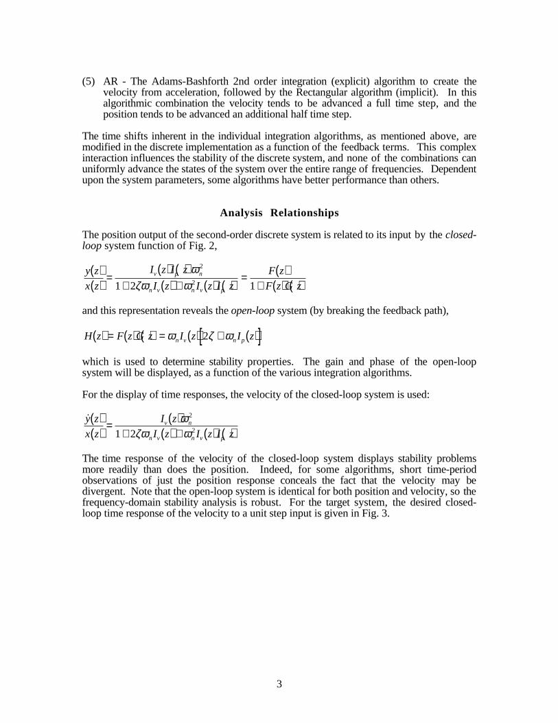
The time response of the velocity of the closed-loop system displays stability problemsmore readily than does the position. Indeed, for some algorithms, short time-periodobservations of just the position response conceals the fact that the velocity may bedivergent. Note that the open-loop system is identical for both position and velocity, so thefrequency-domain stability analysis is robust. For the target system, the desired closed-loop time response of the velocity to a unit step input is given in Fig. 3.

4

40

30

20

10

0V

elo

city

Outp

ut

0.250.200.150.100.050.00

Time - sec

Fig. 3 - Desired Velocity Response

In order to examine the stability of the discrete second order system, the open loop transferfunction is evaluated at the phase crossover frequency, defined as the point where the phaseangle of H z( ) is −π . At this point the gain margin is defined as:

gain margin = when H z z( ) ( ) = −−1 φ π

If the gain margin is less than or equal to unity, the system is unstable. This also meansthat H z( ) is outside the unit circle. The phase margin is defined as how much the phase isabove −π when the gain margin is unity. If the phase margin is not above this value, thenthe system is also unstable.

Note that the closed-loop Laplace function,

y s

x ss

s s

n

n n

( )( )

=+ +

ω

ω ζ ω

2

2

1 2

produces the open-loop Laplace function,

h ss s

n n( ) = +

ω ζ ω2

with phase angle given by,

φ ζωω

=−

−tan 1 2

n

such that the initial phase angle (as ω → 0 ) begins its response in frequency space at thevalue of −π . Phase angles produced in the material given below using z-transforms areadjusted to reflect this fact.

For the “target system” the desired gain and phase of the open-loop system h s( ) are shownin Figs. 4(a) and 4(b).

5

-180

-160

-140

-120

-100

h(s)

Pha

se A

ngle

- D

eg

12 4 6 8

102 4 6 8

1002 4 6 8

1000Frequency - Hz

(b)

80

60

40

20

0

-20

|h(s

)| -

db

12 4 6 8

102 4 6 8

1002 4 6 8

1000Frequency - Hz

(a)

Fig. 4 - Desired Open-Loop Performance

For comparison purposes, these curves are reiterated on other performance figures. Thefive different algorithmic combinations are analyzed in Appendices A through E.

Analysis Results

As a function of the system damping, the algorithmic combinations produce the followingresults in terms of stable discrete processes. The required duty cycle ωnh is produced as afunction of the system damping.

6

Algorithm Program Sequence Damping For Stability

ET˙ ˙ ˙y y hyk k k+ = +1 ζ < 1 2 ω ζnh < 4

y y y yk kh

k k+ += + +( )1 2 1˙ ˙ ζ ≥ 1 2 ω ζnh < 1

ER˙ ˙ ˙y y hyk k k+ = +1

All ω ζ ζnh < + −( )2 1 2

y y hyk k k+ += +1 1˙

TT˙ ˙ ˙ ˙y y y yk k

hk k+ −= + +( )1 2 1 All ω ζ ζ ζnh < + − +( )1 2 1 42 4

y y y yk kh

k k+ += + +( )1 2 1˙ ˙

AT˙ ˙ ˙ ˙y y y yk k

hk k+ −= + −( )1 2 13 ζ < 1 12 See Footnote1

y y y yk kh

k k+ += + +( )1 2 1˙ ˙ ζ ≥ 1 12 ω ζnh < ( )1 2

AR˙ ˙ ˙ ˙y y y yk k

hk k+ −= + −( )1 2 13

All ω ζ ζnh < + −( )2 2 12

y y hyk k k+ += +1 1˙

Table I - Stability Analysis Results

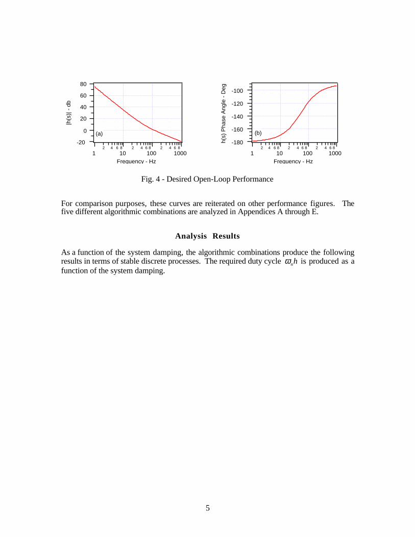
This material is also presented in graphical form in Fig. 5. For each of the integrationcombinations, the discrete model is unstable if the duty cycle is above the pertinent curve.

1 Damping must satisfy ζω ω ω

ω≥

+ + − −9 8 16 4

8

4 4 2 2 2 2n n n

n

h h h

h

7

2.0

1.5

1.0

0.5

0.0

Max

imum

ω

nh

2.01.51.00.50.0Damping (ζ)

ET

ER

TT

AR

Unstable Region

Stable Region

AT

Fig. 5 - Stability Boundaries

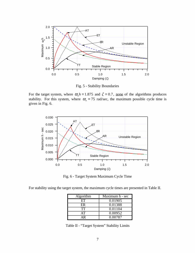
For the target system, where ωnh = 1 875. and ζ = 0 7. , none of the algorithms producesstability. For this system, where ωn = 75 rad/sec, the maximum possible cycle time isgiven in Fig. 6.

0.030

0.025

0.020

0.015

0.010

0.005

0.000

Max

imum

h -

sec

2.01.51.00.50.0Damping (ζ)

ATET

ER

TT

AR

Stable Region

Unstable Region

Fig. 6 - Target System Maximum Cycle Time

For stability using the target system, the maximum cycle times are presented in Table II.

Algorithm Maximum h - secET 0.01905ER 0.01388TT 0.01104AT 0.00952AR 0.00787

Table II - “Target System” Stability Limits

8

From Table II we see that none of the algorithmic combinations are capable of solving thetarget system.

Conclusions

Due to the stability boundaries developed here, the selection of an appropriate integrationsequence for a system with a high natural frequency requires a careful choice. Forexample, a “target system” (representing a real actuator problem) has recently beenpresented to our simulation facility, and this system is too fast to be solved using an arrayof possible algorithms.

Although it appears that a multi-rate procedure is the only solution to the target system(with iaccompanying aliasing problems), a project has recently been completed where analternate algorithmic approach successfully solves the target system. This technique willsoon be published.

9

Appendix A

Euler-Trapezoidal (ET)

Using Euler integration for the acceleration-to-velocity integral followed by trapezoidalintegration for the velocity-to-position integral produces the following code fragment for asecond order system,

˙ ˙

˙ ˙ ˙

˙ ˙

y x y y

y y hy

y y y y

k n k n k n k

k k k

k kh

k k

= − −= +

= + +( )+

+ +

ω ζω ω2 2

1

1 2 1

2

which may be written in z-transform notation by,

˙ ˙

˙ ˙

˙

y z x z y z y z

y zh

zy z

y zh z

zy z

n n n( ) = ( ) − ( ) − ( )

( ) =−

( )

( ) = +( )−( )

( )

ω ζω ω2 22

11

2 1

Hence, for the Euler-Trapezoidal set, the symbolic integrations are given by,

I zh

z

I zh z

z

v

p

( ) =−

( ) = +( )−( )

11

2 1

The closed-loop system for the velocity is given in z-transform notation by,

y z

x z

h

zh

z

h z

z

n

n n

( )( )

= −

+−

+ +( )−( )

ω

ζω ω

2

2 2

2

1

12

11

2 1

and in order to investigate the stability properties, we examine the open-loop function,

H zh

z

h z

z

h

zh z hn n n

n n( ) =−

+ +( )−( )

=−( )

+( ) + −[ ]21

12 1 2 1

4 42 2

2 2

ζω ω ω ω ζ ω ζ

which has a phase angle given by,

φζ ω ω

ω ζ ζ ω ωπ=

−( )+( ) − −( )

−−tan

sin

cos1 4

4 4n

n n

h h

h h h

10

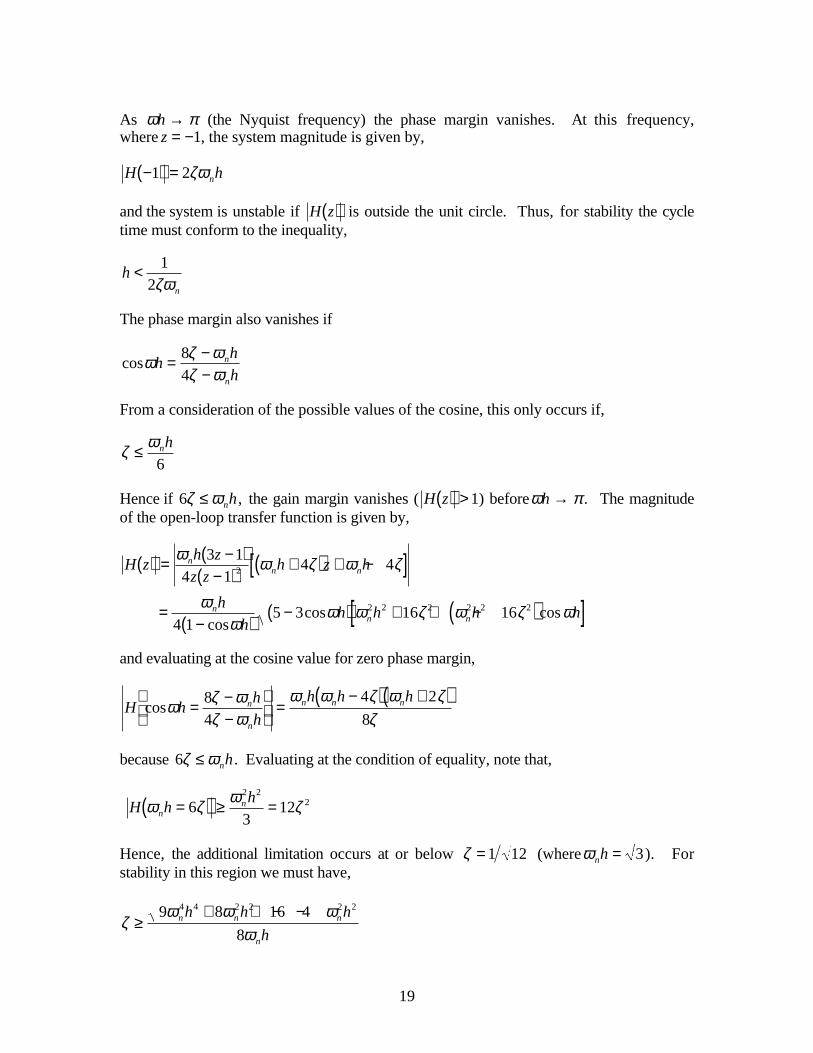
As ω πh → (the Nyquist frequency), the phase margin vanishes. At this frequency, wherez = −1, the system magnitude is given by,

H hn−( ) =1 ζω

The system is unstable if H z( ) > 1 (outside the unit circle). Thus for stability the cycletime must conform to the inequality,

hn

< 1ζω

Also, if 4ζ ω< nh , then φ π≤ − , and the system is unstable.

For a stable system we thus have 1 > ζωnh , and if 4ζ ω< nh , the combination of theseinequalities produces ζ = 1 2. Hence, in the region of lower damping, where 4ζ ω< nh ,for stability the cycle time must conform to the inequality,

hn

< 4ζω

These two inequalities produce a piecewise continuous curve, where the smallest inequalityis required for stability. For a stable Euler-Trapezoidal algorithm we thus have,

h n

n

<<

≥

4 12

1 12

ζω

ζ

ζωζ

Using the given damping and frequency parameters for the target system, the Euler-Trapezoidal scheme is unstable for cycle times above 0.019 seconds. At this cycle time,the magnitude and phase are shown in Figs. A1(a) and A1(b). Considerable deteriorationis shown in phase, as compared to the desired phase of Fig. 4(b).

-180

-160

-140

-120

-100

Pha

se A

ngle

- D

eg

12 4 6 8

102 4 6 8

1002 4 6 8

1000Frequency - Hz

|φ(z)|

|φ(s)|

(b)

ET, with h = 0.019 sec80

60

40

20

0

Mag

nitu

de -

db

12 4 6 8

102 4 6 8

1002 4 6 8

1000Frequency - Hz

|H(z)|

|h(s)|(a)

ET, with h = 0.019 sec

Fig. A1 - Target System Performance, h = 0.019 sec

11

In Fig. A2 the velocity time response is shown to be just barely stable, and is a poorrepresentation of the desired response of Fig. 3.

-100

-50

0

50

100V

eloc

ity R

espo

nse

0.250.200.150.100.050.00

Time - sec

ET Algorithm, h = .019 sec

Fig. A2 - Target System Velocity, h = 0.019

By selecting a cycle time that is half of the maximum value, Fig. A3 is produced. Thedegradation in response is quite noticeable using the ET algorithm with a cycle time that ishalf that required for stability.

50

40

30

20

10

0

Vel

ocity

Res

pons

e

0.250.200.150.100.050.00

Time - sec

ET Algorithm, h = .00975 sec

Fig. A3 - Target System Velocity, h = 0.00975 sec

12

Appendix B

Euler-Rectangular (ER)

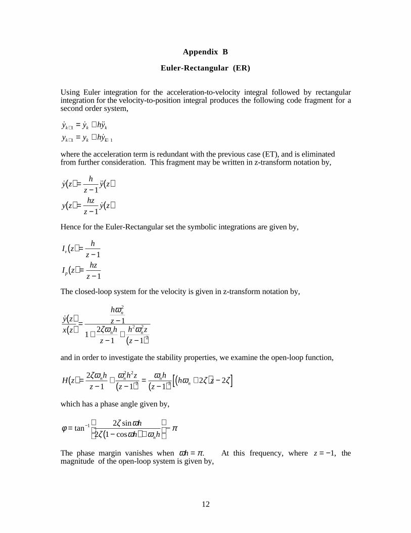
Using Euler integration for the acceleration-to-velocity integral followed by rectangularintegration for the velocity-to-position integral produces the following code fragment for asecond order system,

˙ ˙ ˙

˙

y y hy

y y hyk k k

k k k

+

+ +

= += +

1

1 1

where the acceleration term is redundant with the previous case (ET), and is eliminatedfrom further consideration. This fragment may be written in z-transform notation by,

˙ ˙

˙

y zh

zy z

y zhz

zy z

( ) =−

( )

( ) =−

( )

1

1

Hence for the Euler-Rectangular set the symbolic integrations are given by,

I zh

z

I zhz

z

v

p

( ) =−

( ) =−

1

1


y z

x z

h

zh

z

h z

z

n

n n

( )( )

= −

+−

+−( )

ω

ζω ω

2

2 2

2

1

12

1 1


H zh

z

h z

z

h

zh zn n n

n( ) =−

+−( )

=−( )

+( ) −[ ]21 1 1

2 22 2

2 2

ζω ω ω ω ζ ζ


φ ζ ωζ ω ω

π=−( ) +

−−tan

sincos

1 22 1

h

h hn

The phase margin vanishes when ω πh = . At this frequency, where z = −1, themagnitude of the open-loop system is given by,

13

Hh

hnn−( ) = +( )1

44

ω ω ζand the gain margin is,

gain margin =+( )

44ω ω ζn nh h

At the point of instability this is unity, such that

ω ζ ζnh = + −( )2 1 2

Therefore, the cycle time must conform to the inequality,

hn

<+ −( )2 1 2ζ ζ

ω

Hence, using the given damping and frequency parameters of the target system, the Euler-Rectangular scheme is unstable for cycle times above 0.0138 seconds. At this cycle time,the magnitude and phase are shown in Figs. B1(a) and B1(b). Considerable deteriorationis shown in phase, as compared to the desired phase of Fig. 4(b).

-180

-160

-140

-120

-100

Pha

se A

ngle

- D

eg

12 4 6 8

102 4 6 8

1002 4 6 8

1000Frequency - Hz

|φ(s)|

(b)

ER, with h = 0.0138 sec

|φ(z)|

80

60

40

20

0

Mag

nitu

de -

db

12 4 6 8

102 4 6 8

1002 4 6 8

1000Frequency - Hz

|h(s)|(a)

ER, with h = 0.0138 sec

|H(z)|

Fig. B1 - Target System Performance, h = 0.0138 sec

In Fig. B2 the velocity time response is shown to be just barely stable, and is a poorrepresentation of the desired response of Fig. 3.

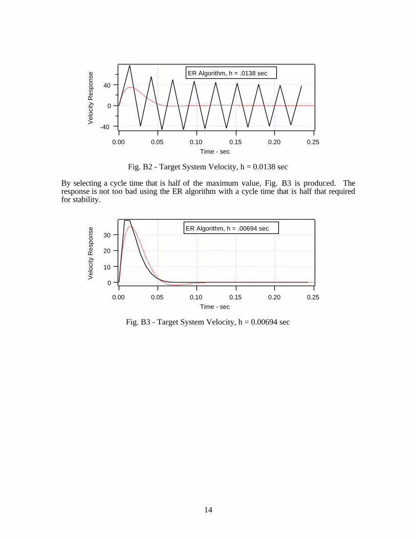
14

40

0

-40

Vel

ocity

Res

pons

e

0.250.200.150.100.050.00

Time - sec

ER Algorithm, h = .0138 sec

Fig. B2 - Target System Velocity, h = 0.0138 sec

By selecting a cycle time that is half of the maximum value, Fig. B3 is produced. Theresponse is not too bad using the ER algorithm with a cycle time that is half that requiredfor stability.

30

20

10

0

Vel

ocity

Res

pons

e

0.250.200.150.100.050.00

Time - sec

ER Algorithm, h = .00694 sec

Fig. B3 - Target System Velocity, h = 0.00694 sec

15

Appendix C

Trapezoidal - Trapezoidal (TT)

Using advanced trapezoidal integration for the acceleration-to-velocity integral followed bytrapezoidal integration for the velocity-to-position integral produces the following codefragment for a second order system,

˙ ˙ ˙ ˙

˙ ˙

y y y y

y y y y

k kh

k k

k kh

k k

+ −

+ +

= + +( )= + +( )

1 2 1

1 2 1

Note that the first trapezoidal process must assume an advance (explicit integration). Thus,it is not strictly “trapezoidal integration,” but could possibly be called “advancingtrapezoidal”. This fragment may be written in z-transform notation by,

˙ ˙

˙

y zh z

z zy z

y zh z

zy z

( ) = +( )−( )

( )

( ) = +( )−( )

( )

12 1

12 1

Hence, for the Trapezoidal-Trapezoidal set, the symbolic integrations are given by,

I zh z

z z

I zh z

z

v

p

( ) = +( )−( )

( ) = +( )−( )

12 1

12 1


y z

x z

h z

z zh z

z z

h z

z z

n

n n

( )( )

=

+( )−( )

+ +( )−( )

+ +( )−( )

ω

ζω ω

2

2 2 2

2

12 1

11

11

4 1


H zh z

z z

h z

z z

h z

z zh z hn n n

n n( ) = +( )−( )

+ +( )−( )

= +( )−( )

+( ) + −[ ]ζω ω ω ω ζ ω ζ11

14 1

14 1

4 42 2 2

2 2


φω ω ω ζ ω

ω ζ ω ζ ωπ=

− + −( )[ ]+( ) + −( )[ ]

−−tan

sin cos

cos cos1

4

1 4 4

h h h h

h h hn n

n

The phase margin vanishes when,

16

cosω ωζ ω

hh

hn

n

=−4

Substituting this into the expression for H z( ) =−11, which is the point at which the system

becomes unstable, produces,

ω ζ ζ ω ζn nh h2 2 2 22 1 2 4 0− +( ) + =

with solution,

ωζ ζ

ζnh =+ − +1 2 1 42 4

producing a gain margin of,

gain margin =+ − +1 2 1 42 4ζ ζ

ζωnh

At the point of instability this is unity. Hence, the cycle time must conform to theinequality,

hn

<+ − +1 2 1 42 4ζ ζ

ζω

Using the given damping and frequency parameters of the target system, the (advanced)Trapezoidal-Trapezoidal scheme is unstable for cycle times above 0.011 seconds. At thiscycle time, the magnitude and phase are shown in Figs. C1(a) and C1(b). Considerabledeterioration is shown in phase, as compared to the desired phase of Fig. 4(b).

-240

-200

-160

-120

Pha

se A

ngle

- D

eg

12 4 6 8

102 4 6 8

1002 4 6 8

1000Frequency - Hz

|φ(s)|

(b)

TT, with h = 0.011 sec

|φ(z)|

80

40

0

-40

Mag

nitu

de -

db

12 4 6 8

102 4 6 8

1002 4 6 8

1000Frequency - Hz

|h(s)|

(a)

TT, with h = 0.011 sec

|H(z)|

Fig. C1 - Target System Performance, h = 0.011 sec

In Fig. C2 the velocity time response is shown to be just barely stable, and is a poorrepresentation of the desired response of Fig. 3.

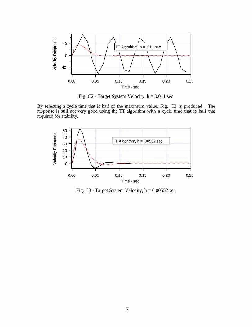
17

40

0

-40Vel

ocity

Res

pons

e

0.250.200.150.100.050.00

Time - sec

TT Algorithm, h = .011 sec

Fig. C2 - Target System Velocity, h = 0.011 sec

By selecting a cycle time that is half of the maximum value, Fig. C3 is produced. Theresponse is still not very good using the TT algorithm with a cycle time that is half thatrequired for stability.

50

40

30

20

10

0Vel

ocity

Res

pons

e

0.250.200.150.100.050.00

Time - sec

TT Algorithm, h = .00552 sec

Fig. C3 - Target System Velocity, h = 0.00552 sec

18

Appendix D

Adams-Bashforth 2nd - Trapezoidal (AT)

Using the Adams-Bashforth 2nd order integration algorithm for the acceleration-to-velocityintegral followed by trapezoidal integration for the velocity-to-position integral produces thefollowing code fragment for a second order system,

˙ ˙ ˙ ˙

˙ ˙

y y y y

y y y y

k kh

k k

k kh

k k

+ −

+ +

= + −( )= + +( )

1 2 1

1 2 1

3


˙ ˙

˙

y zh z

z zy z

y zh z

zy z

( ) = −( )−( )

( )

( ) = +( )−( )

( )

3 12 1

12 1

Hence for the Adams-Trapezoidal set the symbolic integrations are given by,

I zh z

z z

I zh z

z

v

p

( ) = −( )−( )

( ) = +( )−( )

3 12 1

12 1

The closed-loop velocity system is given in z-transform notation by,

y z

x z

h z

z zh z

z z

h z z

z z

n

n n

( )( )

=

−( )−( )

+ −( )−( )

+ +( ) −( )−( )

ω

ζω ω

2

2 2

2

3 12 1

13 1

11 3 1

4 1


H zh z

z z

h z z

z z

h z

z zh z hn n n

n n( ) = −( )−( )

+ +( ) −( )−( )

= −( )−( )

+( ) + −[ ]ζω ω ω ω ζ ω ζ3 11

1 3 14 1

3 14 1

4 42 2

2 2


φω ζ ω ω ω

ζ ω ω ω ωπ

ω ζ ω ζ ω ω

ζ ω ω ζ ω

=−( ) − −( )[ ]

−( ) − +( ) −( )

−

=− − −( )[ ]

− + −( )

−

−

tansin cos cos

cos cos cos

tantan cos

cos

12

1

4 2 1

4 1 1 2

28 4

4 2 4

h h h h

h h h h

hh h h

h h h

n

n

n n

n n

− π

19

As ω πh → (the Nyquist frequency) the phase margin vanishes. At this frequency,where z = −1, the system magnitude is given by,

H hn−( ) =1 2ζω

and the system is unstable if H z( ) is outside the unit circle. Thus, for stability the cycletime must conform to the inequality,

hn

< 12ζω

The phase margin also vanishes if

cosω ζ ωζ ω

hh

hn

n

= −−

84

From a consideration of the possible values of the cosine, this only occurs if,

ζ ω≤ nh

6

Hence if 6ζ ω≤ nh , the gain margin vanishes ( H z( ) > 1) beforeω πh → . The magnitudeof the open-loop transfer function is given by,

H zh z

z zh z h

h

hh h h h

nn n

nn n

( ) = −( )−( )

+( ) + −[ ]

=−( )

−( ) + + −( )[ ]

ω ω ζ ω ζ

ωω

ω ω ζ ω ζ ω

3 14 1

4 4

4 15 3 16 16

2

2 2 2 2 2 2 cos

cos cos

and evaluating at the cosine value for zero phase margin,

H hh

h

h h hn

n

n n ncosω ζ ωζ ω

ω ω ζ ω ζζ

= −−

=−( ) +( )8

4

4 2

8

because 6ζ ω≤ nh . Evaluating at the condition of equality, note that,

H hh

nnω ζ ω ζ=( ) ≥ =63

122 2

2

Hence, the additional limitation occurs at or below ζ = 1 12 (whereωnh = 3). Forstability in this region we must have,

ζω ω ω

ω≥

+ + − −9 8 16 4

8

4 4 2 2 2 2n n n

n

h h h

h

20

These relationships produce a piecewise continuous curve, where the inequalities requiredfor a stable Adams-Trapezoidal algorithm are expressed in terms of the duty cycle:

ζ

ω ω ωω

ζ

ωζ

≥

+ + − −<

≥

9 8 16 4

81 12

12

1 12

4 4 2 2 2 2n n n

n

n

h h h

h

h

Hence, using the given damping and frequency parameters of the target system, theAdams-Trapezoidal scheme is unstable for cycle times above 0.0095 seconds. At this cycletime, the magnitude and phase are shown in Figs. D1(a) and D1(b). Considerabledeterioration is shown in phase, as compared to the desired phase of Fig. 4(b).

-180

-160

-140

-120

-100

Pha

se A

ngle

- D

eg

12 4 6 8

102 4 6 8

1002 4 6 8

1000Frequency - Hz

|φ(s)|

(b)

AT, with h = 0.0095 sec

|φ(z)|

80

60

40

20

0

Mag

nitu

de -

db

12 4 6 8

102 4 6 8

1002 4 6 8

1000Frequency - Hz

|h(s)|(a)

AT, with h = 0.0095 sec

|H(z)|

Fig. D1 - Target System Performance, h = 0.0095 sec

In Fig. D2 the velocity time response is shown to be just barely stable, and is a poorrepresentation of the desired response of Fig. 3.

80

40

0

-40

Vel

ocity

Res

pons

e

0.250.200.150.100.050.00

Time - sec

AT Algorithm, h = .0095 sec

Fig. D2 - Target System Velocity, h = 0.0095 sec

By selecting a cycle time that is half of the maximum value, Fig. D3 is produced. Theresponse is fairly good using the AT algorithm with a cycle time that is half that requiredfor stability..

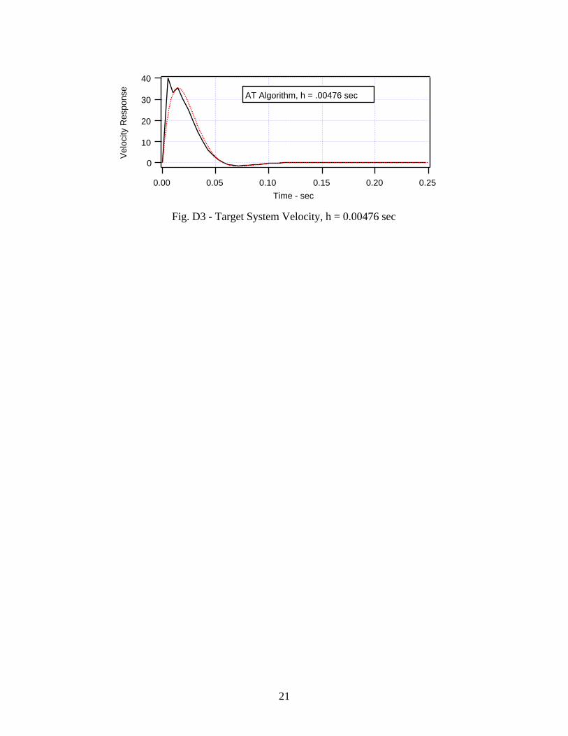
21

40

30

20

10

0

Vel

ocity

Res

pons

e

0.250.200.150.100.050.00

Time - sec

AT Algorithm, h = .00476 sec

Fig. D3 - Target System Velocity, h = 0.00476 sec

22

Appendix E

Adams-Bashforth 2nd - Rectangular (AR)

Using the Adams-Bashforth 2nd order integration algorithm for the acceleration-to-velocityintegral followed by rectangular integration for the velocity-to-position integral producesthe following code fragment for a second order system,

˙ ˙ ˙ ˙

˙

y y y y

y y hy

k kh

k k

k k k

+ −

+ +

= + −( )= +

1 2 1

1 1

3


˙ ˙

˙

y zh z

z zy z

y zhz

zy z

( ) = −( )−( )

( )

( ) =−

( )

3 12 1

1

Hence for the Adams-Rectangular set the symbolic integrations are given by,

I zh z

z z

I zhz

z

v

p

( ) = −( )−( )

( ) =−

3 12 1

1

The closed-loop velocity system is given in z-transform notation by,

y z

x z

h z

z zh z

z z

h z z

z

n

n n

( )( )

=

−( )−( )

+ −( )−( )

+ −( )−( )

ω

ζω ω

2

2 2

2

3 12 1

13 1

13 1

2 1


H zh z

z z

h z z

z z

h z

z zh zn n n

n( ) = −( )−( )

+ −( )−( )

= −( )−( )

+( ) −[ ]ζω ω ω ω ζ ζ3 11

3 12 1

3 12 1

2 22 2

2 2


φω ω ζ ω

ζ ω ω ωπ=

+ −( )[ ]−( ) + −( )

−−tansin cos

cos cos1

2

4 2

4 1 3

h h h

h h hn

n

As ω πh → (the Nyquist frequency), the phase margin vanishes. At this frequency,where z = −1, the system magnitude is given by,

23

Hh

hnn−( ) = +( )1

24

ω ω ζ

H z( ) =−11 is the point at which the system becomes unstable. Evaluating at the point of

instability, this relationship produces the second order equation,

ω ζ ωn nh h( ) + ( ) − =24 2 0

which has only one positive solution. Hence, for stability the cycle time must conform tothe following inequality,

hn

<+ −( )2 2 1

2ζ ζ

ω

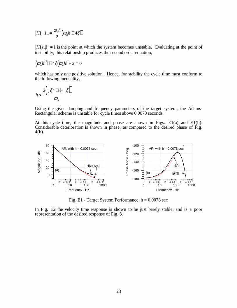
Using the given damping and frequency parameters of the target system, the Adams-Rectangular scheme is unstable for cycle times above 0.0078 seconds.

At this cycle time, the magnitude and phase are shown in Figs. E1(a) and E1(b).Considerable deterioration is shown in phase, as compared to the desired phase of Fig.4(b).

-180

-160

-140

-120

-100

Pha

se A

ngle

- D

eg

12 4 6 8

102 4 6 8

1002 4 6 8

1000Frequency - Hz

|φ(s)|

(b)

AR, with h = 0.0078 sec

|φ(z)|

80

60

40

20

0

Mag

nitu

de -

db

12 4 6 8

102 4 6 8

1002 4 6 8

1000Frequency - Hz

|h(s)|(a)

AR, with h = 0.0078 sec

|H(z)|

Fig. E1 - Target System Performance, h = 0.0078 sec

In Fig. E2 the velocity time response is shown to be just barely stable, and is a poorrepresentation of the desired response of Fig. 3.

24

60

40

20

0

-20Vel

ocity

Res

pons

e

0.250.200.150.100.050.00

Time - sec

AR Algorithm, h = .0078 sec

Fig. E2 - Target System Velocity, h = 0.0078 sec

By selecting a cycle time that is half of the maximum value, Fig. E3 is produced. Theresponse is pretty good using the ER algorithm with a cycle time that is half that requiredfor stability.

30

20

10

0

Vel

ocity

Res

pons

e

0.250.200.150.100.050.00

Time - sec

AR Algorithm, h = .003935 sec

Fig. E3 - Target System Velocity, h = 0.003935 sec

stability of discrete integration algorithms for a real-time

Documents