stability, instability, and bifurcation phenomena in non...

Stability, instability, and bifurcation phenomena in

non-autonomous differential equations

Jose A. Langa†, James C. Robinson‡, Antonio Suarez††Departamento de Ecuaciones Diferenciales y Analisis Numerico, Universidad deSevilla, Apdo. de Correos 1160, 41080-Sevilla, Spain.‡Mathematics Institute, University of Warwick, Coventry, CV4 7AL, U.K.

E-mail: [email protected]; [email protected]; [email protected]

Abstract. There is a vast body of literature devoted to the study of bifurcationphenomena in autonomous systems of differential equations. However, thereis currently no well-developed theory that treats similar questions for the non-autonomous case. Inspired in part by the theory of pullback attractors, we discussgeneralisations of various autonomous concepts of stability, instability, and invariance.Then, by means of relatively simple examples, we illustrate how the idea of a bifurcationas a change in the structure and stability of invariant sets remains a fruitful conceptin the non-autonomous case.

AMS classification scheme numbers: Primary 37G10, 37G35; Secondary , 34D05,34D23.

Submitted to: Nonlinearity

Non-autonomous bifurcation phenomena 2

1. Introduction

The first step in the qualitative theory of autonomous differential equations is an analysis

of fixed points and their stability. This leads on naturally to a study of how the behaviour

near such fixed points can change as a parameter is varied, and this is the genesis of

the whole theory of bifurcations. As one of the main tools in the study of autonomous

systems, this theory is now extremely well developed (see for example Glendinning

(1994) or Guckenheimer and Holmes (1983)). More generally one can start to discuss

stability and bifurcation phenomena associated with more general invariant sets, for

example periodic orbits (e.g. Chow and Hale, 1982).

Such local, and hence relatively “small scale” analysis can be supplemented with

information of a coarser nature concerning the existence of globally attracting sets.

Again, for the autonomous case this approach is well-developed in the theory of global

attractors (Hale, 1988; Ladyzhenskaya, 1991; Robinson, 2001; Temam, 1988). These

are compact, invariant, globally attracting subsets of the phase space which determine

all the asymptotic dynamics. However, only in relatively simple cases are we able to

understand the structure of this attractor in any detail (see Henry (1984) for example).

In this paper we investigate bifurcation phenomena in non-autonomous ordinary

differential equations. Essentially we present a collection of examples which illustrate

some of the problems and, we hope, the sense of the definitions of stability and instability

that we have chosen.

It is clear that for the solution of the non-autonomous equation on Rm

x = f(x, t) x(s) = x0 (1)

the initial time (s) is as important as the final time (t). To treat these equations

as dynamical systems we have to consider a family of solution operators S(t, s)t≥s

(termed a “process” by Sell (1967)) that depend on both the final and initial times. We

can then denote the solution of (1) at time t by S(t, s)x0. If f is sufficiently smooth

then it is clear that S(t, s) : Rm → Rm must satisfy

(i) S(t, t) is the identity for all t ∈ R,

(ii) S(t, τ)S(τ, s) = S(t, s) for all t, τ , and s ∈ R†, and

(iii) S(t, s)x0 is continuous in t, s, and x0.

Note that for an autonomous equation the solution only depends on t − s, so we have

S(t, s) = T (t− s) for some appropriate family T (t)t∈R.If we try to develop a qualitative theory for non-autonomous equations by following

the same route as we would for autonomous systems we immediately find that there are

problems. Indeed, for a generic non-autonomous system we would not expect to find

† When there are solutions of (1) that do not exist for all time some restrictions to the possible valuesof s and t are necessary here: we could define a local process such that for every s there exists at−(s) ≤ 0 and t+(s) > 0 such that S(t, s) is defined for all t− ≤ t ≤ t+. Although we do in fact dealwith equations that generate only local processes in what follows, we will not be too careful about thedistinction between global and local.


any stationary points: if x0 is stationary then this would require that f(x0, t) = 0 for

all t ∈ R. The only candidate we have to replace stationary points is the notion of a

complete trajectory.

Definition 1.1 The continuous map x : R→ Rm is a complete trajectory if

S(t, s)x(s) = x(t) for all t, s ∈ R.

However, in general there will be many complete trajectories, since they are just solutions

that exist for all t ∈ R. For example, if f(x, t) is bounded then any trajectory of (1)

is a complete trajectory. Thus we would expect any complete trajectory that plays an

important role in the dynamics to have very particular stability properties (although we

do not require the concept in this paper, the notion of a hyperbolic trajectory seems the

appropriate one here: see, for example, Malhotra & Wiggins (1998) and (for another

application) Langa et al. (2001)).

A complete trajectory is a particular example of an invariant set in a non-

autonomous equation. We will find this idea particularly useful.

Definition 1.2 A time-varying family of sets Σ(t) is invariant (we say “Σ(·) is

invariant”) if

S(t, s)Σ(s) = Σ(t) for all t, s ∈ R.

This formal definition simply says that if x(s) ∈ Σ(s) then S(t, s)x(s) ∈ Σ(t).

This paper is to our knowledge the first attempt to begin a systematic development

of a theory of bifurcations for non-autonomous equations‡. However, there is already a

substantial body of theory treating attractors for this case (see Kloeden and Schmalfuss

(1997 and 1998), Kloeden and Stonier (1998), and references at the end of this

paragraph). In particular, this theory makes much play with the concept of “pullback

attraction”, where we consider not the asymptotic behaviour of S(t, s) as t → ∞ for

fixed s, but as s → −∞ for fixed t. This is discussed in detail in section 2.1. (In

this paper we restrict our discussion to attractors in Rm, although a similar theory is

possible in a general Banach space, see for example Cheban et al. (2000), Chepyzhov

and Vishik (1994), Crauel et al. (1997), and Schmalfuss (2000)).

‡ There is some previous work couched in the language of skew product flows due to Johnson (1989)and Johnson and Yi (1994) that deals with a generalised notion of Hopf bifurcation about boundedtrajectories of autonomous systems, and Shen and Yi (1998) have discussed the general behaviourof almost periodic scalar differential equations (but make no particular reference to bifurcationphenomena). Both these approaches make use of the fact that the problem can be recast as a skew-product flow over a compact base space, and are not directly applicable to the problems that we considerhere. It may nonetheless be possible to treat the kind of questions that we wish to investigate herewithin this framework by defining an appropriate topology on this base space, as is discussed briefly inthe conclusion.

More immediately relevant is the recent work of Siegmund (2002a & b) who treats the problem offinding normal forms for non-autonomous equations. Just as normal form theory is central for the theoryof bifurcations in autonomous systems, these results could well prove crucial in the non-autonomouscase.


Throughout section 2 we make use of this “pullback” idea to define various notions

of stability and instability which generalise those used in the autonomous case. We can

then begin to discuss non-autonomous bifurcations, where – as in the autonomous case

– we understand this notion as a change in the structure and stability of the invariant

sets of the system.

We present three examples which illustrate our definitions and demonstrate some

of the rich behaviour which can occur in these systems. The first example (section 3) is

a relatively straightforward generalisation of the canonical ODE example of a pitchfork

bifurcation,

x = ax− b(t)x3 x ∈ R,

and, by means of an exact solution, we obtain very similar behaviour. Next (in section

4) we consider how a change of linear stability near the origin effects the behaviour of

the system

u = Au + F (u; t) u ∈ Rm,

assuming that Au contains all the linear terms: for the particular case when F

contributes to the dissipation we outline a bifurcation from 0 to a non-trivial attractor.

Finally in section 5 we investigate a non-autonomous version of the canonical saddle-

node example,

x = a− b(t)x2 x ∈ R.

This equation requires an analysis that is “essentially non-autonomous” since there is

no stationary solution, and exhibits some features unique to such models (for example,

we obtain an asymptotically unstable set which is not a subset of the attractor). The

dynamics can be described by means of a pair of complete trajectories with well-defined

stability properties.

In the conclusion we summarise and consider how one might develop the theory

further in a systematic way.

2. Notions of attraction and stability

We wish to define the non-autonomous equivalents of various concepts of stability

familiar from the theory of autonomous systems. We start with the notion of attraction,

since it is the theory of non-autonomous attractors (see section 2.3) that has inspired

much of our approach.

In what follows we make constant use of the Hausdorff semidistance between two

sets A and B, dist(A,B), which is defined as

dist(A,B) = supa∈A

infb∈B

d(a, b) :

note that this only measures how far A is from B (dist(A,B) = 0 only implies that

A ⊆ B). We also use the notation N(X, ε) to denote the ε-neighbourhood of a set X:

N(X, ε) = y : y = x + z, x ∈ X, z ∈ Rm with |z| ≤ ε.


2.1. Attraction

In autonomous systems, an invariant set Σ is (locally) attracting (or “quasi-

asymptotically stable”, Glendinning (1994)) if there exists a neighbourhood O of Σ

such that

dist(S(t, 0)x0, Σ) → 0 as t →∞, for all x0 ∈ O. (2)

(Of course, in an autonomous system the initial time is not important, but we make the

dependence explicit here to facilitate our discussion.)

Indeed, we are accustomed to considering “time-asymptotic” behaviour as the

limiting behaviour as t → ∞. The “practical” implication of this idea is, however,

that if we run an experiment for long enough and then consider the state of the system

at some future time, it is well approximated by one of the states in the attractor.

In the autonomous case, where S(t, s) = T (t−s), the concept of attraction in (2) is

entirely equivalent to the existence of a neighbourhood O of Σ such that for each fixed

t ∈ R,

dist(S(t, s)x0, Σ) → 0 as s → −∞, for all x0 ∈ O. (3)

This idea of “pullback” attraction (cf. Kloeden and Schmalfuss, 1998; Schmalfuss, 2000)

does not involve running time backwards: rather, we consider taking measurements in

an experiment now (at time t) which began some time in the past (at time s < t). If

the experiment has been running long enough, we expect once again that the state of

the system is well approximated by one of the “attracting states”.

It turns out that for non-autonomous systems this idea of “pullback attraction” is

much more natural than the more familiar “forward” attraction of (2). One advantage is

that the pullback procedure allows us to consider “time-asymptotic behaviour” without

having to consider sets Σ(t) that are moving (and perhaps become unbounded), since

the final time is fixed. A clear example of this is given in proposition 3.1, where the

attracting orbit (given explicitly in (10)) is unbounded as t → +∞.

This approach has proved extremely fruitful, particular in the study of stochastic

differential equations (Crauel and Flandoli, 1994; Crauel et al., 1997; Schmalfuss, 1992)

and has already found application is the study of non-autonomous ODEs (Kloeden and

Schmalfuss, 1998; Kloeden and Stonier, 1998) and PDEs (Langa and Robinson 2001;

Langa and Suarez, 2001; Cheban et al., 2000).

We will therefore make all our definitions “in the pullback sense”. For some similar

definitions for non-autonomous systems, but made “forwards in time” see Hale (1969).

Definition 2.1 We say that Σ(·) is (locally) pullback attracting if for every t ∈ R there

exists a δ(t) > 0 such that if

lims→−∞

dist(x(s), Σ(s)) < δ(t)

then

lims→−∞

dist[S(t, s)x(s), Σ(t)] = 0. (4)


Note that it is crucial that in the definition here, δ is not allowed to depend on

s, otherwise – due to continuous dependence on initial conditions – every invariant set

would be pullback attracting.

There are many possible definitions of what it might mean to be “globally pullback

attracting” in a non-autonomous system, since the pullback procedure allows the “initial

condition” to vary with s. All such definitions can be put into a coherent framework by

defining a “universe” of sets which we require to lie in the basin of attraction of any set

which we would like to call “an attractor” (the details of this idea are given in Flandoli

and Schmalfuss (1996), Schenk-Hoppe (1998), and Schmalfuss (1992) in the stochastic

case, and by Schmalfuss (2000) for non-autonomous systems). However, the following

definition, which fixes the initial condition, seems to be the most appropriate.

Definition 2.2 An invariant set Σ(·) is globally pullback attracting if for every t ∈ Rand every x0 ∈ Rm,

lims→−∞

dist[S(t, s)x0, Σ(t)] = 0.

[As an illustration of the many other possible definitions, let us call a set “uniformly

pullback attracting” if (4) in definition 2.1 holds for any δ > 0. The simple autonomous

ODE x = −x serves to illustrate the distinction between “uniform” and “global”

pullback attraction. Since the solution of this equation that satisfies x(s) = xs is

x(t, s; xs) = xse−(t−s) = e−(t−s)[xs − αe−s] + αe−t

for any α ∈ R, it follows that every solution αe−t is uniformly pullback attracting (we

take an xs with |xs − αe−s| ≤ δ), while only the zero solution is globally pullback

attracting (we fix xs).]

2.2. Stability

Standard definitions of asymptotic stability have two components. One is attraction,

which we have already discussed in detail above, and the other is “Lyapunov stability”,

which constrains trajectories to stay close to the invariant set. We now give these

definitions in the non-autonomous case.

Definition 2.3 Σ(·) is pullback Lyapunov stable if for every t ∈ R and ε > 0

there exists a δ(t) > 0 such that for any s < t, xs ∈ N(Σ(s), δ(t)) implies that

S(t, s)xs ∈ N(Σ(t), ε).

It is easy to verify that this agrees with the usual definition in the autonomous case.

Combining this with pullback attraction we obtain a definition of pullback

asymptotic stability.

Definition 2.4 We say that Σ(·) is locally (globally) pullback asymptotically stable if

it is both pullback Lyapunov stable and locally (globally) pullback attracting.


2.3. Pullback attractors

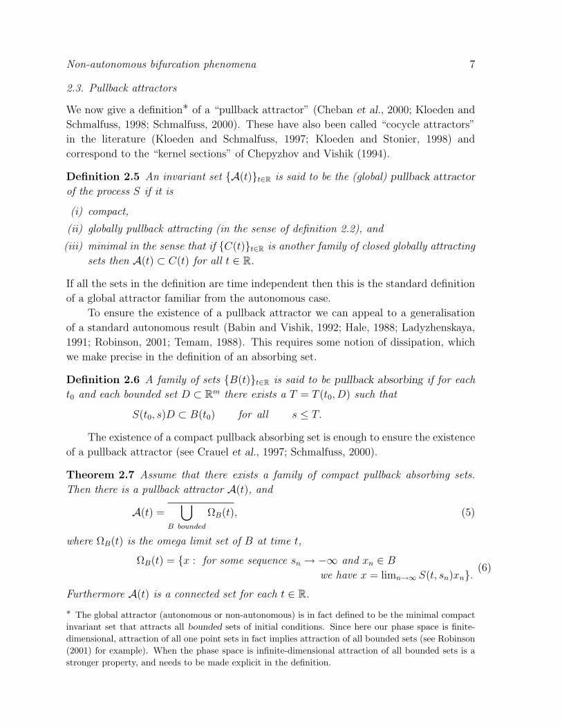
We now give a definition∗ of a “pullback attractor” (Cheban et al., 2000; Kloeden and

Schmalfuss, 1998; Schmalfuss, 2000). These have also been called “cocycle attractors”

in the literature (Kloeden and Schmalfuss, 1997; Kloeden and Stonier, 1998) and

correspond to the “kernel sections” of Chepyzhov and Vishik (1994).

Definition 2.5 An invariant set A(t)t∈R is said to be the (global) pullback attractor

of the process S if it is

(i) compact,

(ii) globally pullback attracting (in the sense of definition 2.2), and

(iii) minimal in the sense that if C(t)t∈R is another family of closed globally attracting

sets then A(t) ⊂ C(t) for all t ∈ R.

If all the sets in the definition are time independent then this is the standard definition

of a global attractor familiar from the autonomous case.

To ensure the existence of a pullback attractor we can appeal to a generalisation

of a standard autonomous result (Babin and Vishik, 1992; Hale, 1988; Ladyzhenskaya,

1991; Robinson, 2001; Temam, 1988). This requires some notion of dissipation, which

we make precise in the definition of an absorbing set.

Definition 2.6 A family of sets B(t)t∈R is said to be pullback absorbing if for each

t0 and each bounded set D ⊂ Rm there exists a T = T (t0, D) such that

S(t0, s)D ⊂ B(t0) for all s ≤ T.

The existence of a compact pullback absorbing set is enough to ensure the existence

of a pullback attractor (see Crauel et al., 1997; Schmalfuss, 2000).

Theorem 2.7 Assume that there exists a family of compact pullback absorbing sets.

Then there is a pullback attractor A(t), and

A(t) =⋃

B bounded

ΩB(t), (5)

where ΩB(t) is the omega limit set of B at time t,

ΩB(t) = x : for some sequence sn → −∞ and xn ∈ B

we have x = limn→∞ S(t, sn)xn. (6)

Furthermore A(t) is a connected set for each t ∈ R.

∗ The global attractor (autonomous or non-autonomous) is in fact defined to be the minimal compactinvariant set that attracts all bounded sets of initial conditions. Since here our phase space is finite-dimensional, attraction of all one point sets in fact implies attraction of all bounded sets (see Robinson(2001) for example). When the phase space is infinite-dimensional attraction of all bounded sets is astronger property, and needs to be made explicit in the definition.


Although there are essential differences between the concepts of autonomous global

attractors and pullback attractors, they are related: it is shown in Caraballo and Langa

(2001) that if a family of non-autonomous processes Sσ(t, s) converge to an autonomous

flow S(t− s) as σ → 0 and there is some uniformity in the size of the absorbing set for

0 ≤ σ ≤ σ0, then dist(Aσ(t),A) → 0 as σ → 0, where Aσ(t) is the pullback attractor

for Sσ(t, s) and A is the global attractor for S(t − s). Indeed, this result is a further

piece of evidence that the pullback definition of attraction (and, we hope, stability) is

entirely consistent with more familiar autonomous ideas. (A special case of this result

is discussed at the end of section 3.)

2.4. Instability

We define local pullback instability as the converse of pullback Lyapunov stability.

Definition 2.8 We say that Σ(·) is locally pullback unstable if it is not pullback

Lyapunov stable, i.e. if there exists a t ∈ R and an ε > 0 such that, for each δ > 0,

there exists an s < t and an x0 ∈ N(Σ(s), δ) such that

dist(S(t, s)x0, Σ(t)) > ε.

However, a more natural concept from a dynamical point of view is the idea of an

“unstable set”, defined by Crauel (2001) for the case of random dynamical systems

(which also necessitate the pullback concept of attraction) just as for autonomous

deterministic systems (see Temam (1988) for example).

Definition 2.9 If Σ(·) is an invariant set then the unstable set of Σ, UΣ(·), is defined

as

UΣ(s) = u : limt→−∞

dist (S(t, s)u, Σ(t)) = 0.We say that Σ(·) is asymptotically unstable if for some t we have

UΣ(t) 6= Σ(t). (7)

Since we always have Σ(t) ⊂ UΣ(t) when Σ(·) is invariant, (7) says that Σ(t) is a strict

subset of UΣ(t) – in this case we will say that UΣ(t) is “non-trivial”.

Note that the instability of Σ(t) is equivalent to the stability (in the usual, forward,

sense) of Σ(−t) for the time-reversed system. This introduces a lack of symmetry in

the definitions, since the pullback procedure is not involved here. However, if Σ(·) has

a non-trivial unstable set then it is “unstable” in a strong sense, as the following result

shows.

Proposition 2.10 If Σ(·) is asymptotically unstable then it is also locally pullback

unstable and cannot be locally pullback attracting.

Proof. Since Σ(·) is asymptotically unstable there exists an s and an element x ∈ UΣ(s)

such that

dist(x, Σ(s)) > ε > 0


for some ε > 0. However, xt = S(t, s)x satisfies

limt→−∞

dist(xt, Σ(t)) = 0.

Given a δ > 0, it follows that we can choose t0 small enough that

dist(xt, Σ(t)) < δ, for all t ≤ t0.

Since this holds for all t ≤ t0 it follows that Σ(·) is not locally pullback attracting, and

choosing any particular t < t0 shows that Σ(·) is locally pullback unstable. ¤We observe here that in an autonomous or random dynamical system, the unstable

set of any invariant set must be a subset of the attractor (see Robinson (2001), Stuart

and Humphries (1996), or Temam (1988) for the autonomous case and Crauel (2001) for

the random case). For non-autonomous systems we can only prove a similar result when

Σ(t) is bounded on each semi-infinite time interval (−∞, t]. An example of a system

with an asymptotically unstable invariant set which is not a subset of the attractor is

given in section 5.

Proposition 2.11 Suppose that Σ(·) is invariant and that⋃

s∈(−∞,t]

Σ(s)

is contained in a bounded set B(t) for each t ∈ R. Then UΣ ⊂ A.

Proof. If x ∈ UΣ(s) then it follows that there exists a t0(ε, x) such that for all t ≥ t0

dist(u(−t, s; x), Σ(−t)) ≤ ε.

In particular it follows that for all such t the solution u(−t, s; x) is contained in

the bounded set B = N(B(s), ε). Thus we can write x = S(s,−tn)yn, where

yn = S(−tn, s)x ∈ B and tn → ∞. It follows (see (6)) that x ∈ ΩB(s), and hence

is an element of A(s). ¤

2.5. The concept of bifurcation in non-autonomous systems

Given the above definitions, we can discuss in a meaningful way the idea of a bifurcation

in a non-autonomous system. Exactly as in the autonomous case, a bifurcation is a

change in the stability and structure of the invariant sets of the system. This covers a

multitude of sins, but in what follows we will concentrate on non-autonomous versions

of the most simple bifurcation phenomena.

In our first two examples we will observe only local bifurcation phenomena in a

neighbourhood of the origin: indeed, we will make the very strong assumption that zero

is a stationary point for all values of the parameter. We give a non-autonomous version

of the pitchfork bifurcation, and then a more general bifurcation scenario based on the

linearised equation near zero. In some cases this second bifurcation can be understand

in terms of the appearance of a non-trivial attractor.

Then we consider a non-autonomous version of the saddle-node bifurcation, which

illustrates some of the rich behaviour possible in the non-autonomous case.


3. A non-autonomous pitchfork bifurcation

The canonical autonomous example of an equation exhibiting a pitchfork bifurcation

(see Glendinning, 1994) is

x = ax− bx3 b > 0. (8)

When a < 0 the origin is locally stable, while for a > 0 the origin becomes unstable and

two new stable fixed points appear at ±√

b/a. For a < 0 the global attractor is just

0, while for a > 0 the global attractor is the interval [−√

b/a,√

b/a].

In this section we study a non-autonomous version of (8). (This was also studied

in Caraballo and Langa (2001) with the emphasis on its attractor.)

Proposition 3.1 Consider the equation

x = ax− b(t)x3 x(s) = xs, (9)

under the assumption that 0 < b(t) ≤ B. For a < 0 the origin is globally asymptotically

pullback stable, while for a > 0 the origin becomes asymptotically unstable and two new

locally asymptotically pullback stable complete trajectories ±α(t; a) appear, where

α2(t; a) =e2at

2∫ t

−∞ e2aτb(τ)dτ. (10)

Note that if b(t) → 0 then α(t; a) →∞ as t → +∞.

[One could use this result directly to give a simple example of a non-autonomous

version of the Hopf bifurcation by considering the system

r = ar − b(t)r3 θ = ω,

where (r, θ) are polar coordinates in R2 (cf. Glendinning (1994) in the autonomous

case).]

Proof. By means of the substitution y = x−2 this equation admits an exact solution:

for xs > 0

x(t)2 =e2at

e2asx−2s + 2

∫ t

se2arb(r) dr

. (11)

For a < 0 we can define a global attractor as in the autonomous case: when t tends

to +∞ all solutions are attracted to the point 0. The pullback attractor is also just

0, since this is the limit of (11) when s tends to −∞.

On the other hand when a > 0 all solutions are unbounded as t → ∞ if b(t) → 0

as t → ∞. However, we can always define the pullback attractor. Indeed, taking the

limit as s → −∞ in (11) yields

α2(t; a) =e2at

2∫ t

−∞ e2aτb(τ)dτ, (12)

and it is easy to check that α(·; a) is a complete trajectory of (9) (see definition 1.1).


The construction of α(t; a) ensures that it is pullback attracting. If we rearrange

(11) as

x2(t) =e2at

e2as[x−2(s)− α−2(s; a)] + 2∫ t

−∞ e2arb(r) dr

then pullback Lyapunov stability follows easily and it is clear that any solution S(t, s)xs

with xs < α(s; a) converges to 0 as t → −∞. ¤We could rephrase this result in terms of attractors (the equation is treated this

way in Caraballo and Langa, 2001): for a < 0 the pullback attractor is just the origin,

while for a > 0 it is the interval [−α(t; a), α(t; a)]. In this context it is interesting to

observe that if we consider a family of non-autonomous problems

x = ax− bσ(t)x3

where for each σ > 0 the function bσ(t) satisfies the conditions of proposition 3.1,

but with bσ(t) → b (constant) uniformly on bounded sets, it is easy to see that

α(t; a, σ) →√

a/b for each t and in the limit we recover the global attractor for the

autonomous problem

x = ax− bx3.

(A general result along these lines, due to Caraballo and Langa (2001), was discussed

briefly at the end of section 2.3.)

4. A bifurcation deduced from the linearised equation

We now consider a more complicated example which we cannot solve explicitly, and

investigate what happens when the linearised flow at the origin (which we assume is

autonomous) changes its stability. We consider the system for u ∈ Rm

u = Au + F (u; t), (13)

where

• A is a real m×m matrix of the form

A =

(λ 0

0 −A

),

with A a real (m− 1)× (m− 1) matrix that satisfies

yT Ay ≥ µ|y|2 for all y ∈ Rm−1,

• F (0, t) = 0 for all t ∈ R,

• for some p > 0

|F (u; t)− F (v; t)| ≤ a(t)[|u|2p + |v|2p]|u− v|, (14)

where for each t ∈ Rsup

s∈(−∞,t]

a(s) = α(t) < ∞. (15)


Note that the two properties of F above together imply that

|F (u; t)| ≤ a(t)|u|2p+1. (16)

4.1. Local pullback asymptotic stability when λ < 0.

First we consider the case when λ < 0, for which the origin is linearly stable, and prove

that it must also be locally pullback asymptotically stable.

Proposition 4.1 If λ < 0 the origin is locally pullback asymptotically stable.

Proof. Setting κ = min(µ,−λ) it follows that xTAx ≤ −κ|x|2. Using this bound and

(16) it follows that1

2

d

dt|u|2 ≤ −κ|u|2 + a(t)|u|2p+2.

With the substitution θ(t) = |u(t)|−2p the corresponding differential inequality

dθ

dt≥ 2κpθ − 2pa(t)

can be solved explicitly to give

θ(t) ≥ e2κpt

[e−2κpsθ(s)− 2p

∫ t

s

e−2κpra(r) dr

].

Using condition (15) it follows that

∫ t

s

e−2κpra(r) dr ≤ α(t)

2κpe−2κps,

and so provided that θ(s) = θ0 > α(t)/κ, we have θ(t) → ∞ as s → −∞ and hence

0 is locally pullback attracting. The origin is also pullback Lyapunov stable, since

choosing θ(s) ≥ ε−2p + (α(t)/κ) ensures that θ(t) ≥ ε−2p for all t ≥ s. ¤

4.2. Asymptotic instability when λ > 0

To show asymptotic instability when λ > 0 we follow the idea of the proof in Caraballo

et al. (2001) and prove the existence of a local unstable manifold near the origin. In

what follows we consider (13) in its equivalent form for (x, y) ∈ R× Rm−1,

x = λx + f(x, y; t)

y = − Ay + g(x, y; t).

Proposition 4.2 If λ > 0 then the origin is asymptotically unstable. In particular,

there exists a Lipschitz function φ : R× R→ Rm−1 and a %(t) > 0 such that the set

M(s) = (xs, φ(xs, s)) : |xs| ≤ %(s)

forms part of the unstable set of 0.


Proof. Using a contraction mapping argument we find an invariant manifold in a small

neighbourhood on the origin. First we truncate the nonlinear term to ensure that its

Lipschitz constant is uniformly small.

We take a smooth function θ : [0,∞) → [0, 1] satisfying

θ(r) = 1 0 ≤ r ≤ 1, |θ′(r)| ≤ 2 1 ≤ r ≤ 2 θ(r) = 0 r ≥ 2

we truncate the nonlinear term in a ball of radius δ(t),

Fδ(u; t) = θ

( |u|δ(t)

)F (x, y; t).

It follows (cf. Temam, 1988) that

|Fδ(u; t)− Fδ(v; t)| ≤ Ca(t)δ(t)2p|u− v|.

We now take δ(t)2p = ε[Cα(t)]−1 (note that δ(t) is non-increasing in t) so that

|Fδ(u; t)− Fδ(v; t)| ≤ ε|u− v| and |Fδ(u; t)| ≤ ε|u|. (17)

We look for an invariant manifold for the truncated equation

u = Au + Fδ(u; t). (18)

We will write (fδ(u; t), gδ(u; t)) for the corresponding nonlinear terms in the separated

(x, y) equations.

We now define a mapping T on the collection L of Lipschitz functions φ : R×R→Rm−1 that satisfy

|φ(x, t)− φ(y, t)| ≤ |x− y|,equipped with the usual supremum norm (‖φ‖∞ = sup(x,t)∈R×R |φ(x, t)|). For φ ∈ L we

define [Tφ](xs, s) as the solution at time s of the y equation in the partially coupled

system

x = λx + fδ(x, φ(x, t); t) x(s) = xs

y = −Ay + gδ(x, φ(x, t); t) limt→−∞

y(t) = 0.

¿From the explicit form for the solution of the y equation between s an t,

y(t) = e−A(t−s)y(s) +

∫ t

s

e−A(t−r)gδ(x(r), φ(x(r), r)) dr, (19)

and the bound on gδ as in (17) it follows that

[Tφ](xs, s) =

∫ s

−∞e−A(s−r)gδ(x(r), φ(x(r), r); r) dr. (20)

The graph of a fixed point φ of T ,

(x, φ(x)) : x ∈ R


corresponds to an invariant manifold for the truncated equation (18) – this can be shown

by substituting the expression (x(t), φ(x(t), t)) into (19) and then using the fact that

Tφ = φ.

First we check that Tφ ∈ L. We have

|[Tφ](xs, s)− [Tφ](xs, s)|=

∣∣∣∣∫ s

−∞e−A(s−r)[gδ(x(r), φ(x(r), r); r)− gδ(x(r), φ(x(r), r); r)] dr

∣∣∣∣

≤∫ s

−∞εe−µ(s−r)2|x(r)− x(r)| dr.

Easy estimates on the difference of two solutions of

x = λx + fδ(x, φ(x, t); t)

yield

|x(r)− x(r)| ≤ e(λ−2ε)(r−s)|xs − xs|,and so we require

ε

∫ s

−∞e−[µ+λ−2ε](s−r) dr ≤ 1.

This follows for every s if ε is sufficiently small.

To show that T is a contraction we consider

|[Tφ](xs)− [T φ](xs)|=

∣∣∣∣∫ s

−∞e−A(s−r)[gδ(x(r), φ(x(r), r); r)− gδ(x(r), φ(x(r), r); r)] dr

∣∣∣∣

≤∫ s

−∞e−µ(s−r)ε

[2|x(r)− x(r)|+ ‖φ− φ‖∞

]dr.

Again, relatively straightforward estimates comparing the solutions of

dx/dt = λx + fδ(x, φ(x, t); t) and dx/dt = λx + fδ(x, φ(x, t); t)

yield, provided that λ > 2ε,

|x(r)− x(r)| ≤ ε‖φ− φ‖∞λ− 2ε

,

so that

|[Tφ](xs, s)− [T φ](xs, s)| ≤ λε

µ(λ− 2ε)‖φ− φ‖∞,

which shows that T is a contraction for ε sufficiently small.

We now show that if |xs| ≤ %(s) = δ(s)/2√

2 then us = (xs φ(xs)) ∈ Σ[0](s).

Indeed, on the graph of φ(x, t) the equation reduces to

x = λx + fδ(x, φ(x, t); t).


Then, if t = −τ , we have

d|x|/dτ ≤ −λ|x|+ 2ε|x| = −(λ− 2ε)|x|.

It follows that

|x(t)| ≤ e(λ−2ε)(t−s)|x(s)|.Since y(t) = φ(x(t), t) we have |u(t)| ≤ √

2|x(t)|. Since δ(t) is non-increasing, it follows

that if |xs| ≤ δ(s)/2√

2 then |u(t)| ≤ δ(t) < 2 for all t ≤ s: in particular the solution

u(t) is also a solution of the original, untruncated equation, and so xs ∈ Σ[0](s). ¤

4.3. A bifurcation to a non-trivial pullback attractor

We note here that if the nonlinear term in fact contributes to the dissipation, so that

(F (u; t), u) ≤ −a(t)|u|2p+2,

then for λ < 0 the origin is globally pullback asymptotically stable. However for λ > 0

proposition 4.2 still applies. It follows that while for λ < 0 the pullback attractor is just

the origin, for λ > 0 this attractor is non-trivial since (using proposition 2.11 and the

fact that 0 is bounded) it must contain M(·) which is a subset of the unstable set of

0. It should be relatively simple to demonstrate this kind of bifurcation behaviour in

complicated systems where a more detailed description is extremely difficult.

5. A non-autonomous saddle-node bifurcation

Our final example is a non-autonomous version of the saddle-node bifurcation. The

simplest autonomous example which exhibits this bifurcation is

x = a−Bx2

(see Glendinning (1994) for example). Clearly this equation has no fixed points for

a < 0, while for a > 0 there are two fixed points ±√

a/B: if x0 < −√

a/B then

x(t) → −∞ in finite time, while if x0 > −√

a/B then x(t; x0) →√

a/B as t → +∞.

In this section we consider the non-autonomous equation

x = a− b(t)x2 (21)

where 0 < b(t) ≤ B, b(t) → 0 as |t| → ∞, and∫ 0

−∞b(s) ds =

∫ ∞

0

b(s) ds = ∞. (22)

The invariance of these conditions when t 7→ −t greatly simplifies the analysis.


5.1. Behaviour for a ≤ 0

First we consider the simple cases a ≤ 0 where the behaviour is essentially the same as

in the autonomous case.

Lemma 5.1 If a < 0 then every solution S(t, s)x0 tends to −∞ in a finite time, both

“forwards” (fix s and x0 and let t → t∗ < +∞) and “pullback” (fix t and x0 and let

s → s∗ > −∞). If a = 0 then solutions with x0 > 0 tend to zero (forwards and pullback)

while if x0 < 0 then S(t, s)x0 tends to −∞ in finite time (as in the case a < 0).

Proof. When a = 0 the equation can be solved explicitly to yield

S(t, s)xs =xs

1 + xs

∫ t

sb(r) dr

:

the behaviour described in the statement of the lemma is immediate. ¤

5.2. Saddle-node type behaviour for a > 0

We now show that when a > 0 there are two complete trajectories which we can identify

as being “stable” and “unstable”.

Theorem 5.2 For a > 0 there exist two complete trajectories of (21) α(t) and β(t)

which are bounded below (resp. above) by√

a/B (resp. −√

a/B) and diverge to +∞(resp. −∞) as |t| → ∞. The solution α(t) is globally pullback asymptotically stable and

the solution β(t) is asymptotically unstable:

lims→−∞ x(t, s; x0) = α(t) ∀ x0

limt→−∞[x(t, s; x0)− β(t)] = 0 ∀ x0 < α(s).(23)

We also have††limt→+∞[x(t, s; x0)− α(t)] = 0 ∀ x0 > β(s)

lims→+∞ x(t, s; x0) = β(t) ∀ x0.(24)

Note that the global pullback stability of α(t) in (23) shows that α(t) is the pullback

attractor. Nevertheless, the complete orbit β(t) plays an important role in the dynamics

if we consider the asymptotic behaviour as t → ∞. Indeed, the system provides an

example in which there exists an invariant set with a non-trivial unstable set which

is nevertheless not a subset of the attractor (here the trajectory β(t) is unbounded as

t → −∞, and so falls outside the conditions of proposition 2.11).

Proof. We investigate the behaviour of solutions S(t, s)x0 when s → −∞. First note

that if t and x0 are fixed then there exists an s0(t, x0) such that the solution is bounded

below,

S(t, s)x0 >√

a/B for all s ≤ s0. (25)

††We have so far resisted the temptation of defining a notion of “pullback instability” as “pullbackbackwards stability”, cf. lims→+∞ x(t, s; x0) = β(t).


Indeed, choose ε(x0) < B small enough that x0 > −√

a/ε. Then there exists a time

τ(ε) such |b(t)| ≤ ε for all t ≤ τ(ε), and so

x ≥ a− εx2 for all t ≤ τ(ε).

Now, there exists a time T such that the solution of

y = a− εy2 y(0) = x0

satisfies y(t) ≥√

a/B for all t ≥ T . Thus if we take s ≤ s0 ≡ τ(ε)− T we obtain (25).

Now set

β = infr∈[t−1,t]

b(r).

Then on the time interval [t− 1, t] we have

x ≤ a− βx2.

It follows (see Temam (p87 in 1988 1st edition or p89 in 1996 2nd edition) that for all

s ≤ s0− 1 the solution S(t, s)x0 is also bounded above independently of the value of x0,

so we have

√a/B ≤ S(t, s)x0 ≤

√a/β + β−1 for all s ≤ s0 − 1.

It follows from theorem 2.7 that there exists a pullback attractor A(t), which for

each t ∈ R is a connected set. Since A(t) is a subset of R

A(t) = [α(t), α+(t)]

for some α(t) and α+(t). Since the phase space is one-dimensional the process is order-

preserving and so α(t) and α+(t) are trajectories of (21).

Note that it follows from (25) that α(t) ≥√

a/B for all t. In consequence

α(t) → +∞ as t → −∞. (26)

To show this consider the time-reversed problem with τ − t: writing α′ = dα/dτ we

have

α′ = −a + b(−τ)α2.

Suppose that (26) does not hold, so that there exists a k such that for each τ0 there

exists a τ ≥ τ0 with α(τ) ≤ k. Choose ε small enough that k <√

a/ε, and then T such

that for all τ ≥ T , b(−τ) ≤ ε. It follows that for all τ ≥ T we have

α′ ≤ −a + εα2,

and so in particular, since α(τ) ≤ k <√

a/ε for some τ ≥ T ,

limτ→∞

α(τ) ≤ −√

a/ε <√

a/B,


and we obtain (26) by contradiction.

In particular for all x0 we have x0 < α(s) for s small enough. Since S(t, s) is

order-preserving and α(t) is a complete trajectory, it is a consequence of the pullback

attraction property of A(t),

lims→−∞

dist[S(t, s)x0,A(t)] = 0,

that we must have

lims→−∞

S(t, s)x0 = α(s),

and this implies that A+(t) = α(t).If we now consider the system with both time and space reversed (y = −x and

τ = −t) the symmetry of the conditions on b(t) allows us to use exactly the same

arguments to prove the existence a complete trajectory β(t) such that β(t) ≤ −√

a/B,

β(t) → −∞ as |t| → ∞, and

lims→∞

S(t, s)x0 = β(t) (27)

for all x0.

It only remains to prove the second part of (23) or (24): we choose to prove the

second part of (24), taking an x0 > β(s). Note that if we take any two initial conditions

x0 and y0 and consider the two solutions of (21) x(t) = S(t, s)x0 and y(t) = S(t, s)y0

then their difference z(t) = x(t)− y(t) satisfies

z = −b(t)[x(t) + y(t)]z,

so that

z(t) = |x0 − y0| exp

(−

∫ t

s

[x(r) + y(r)]b(r) dr

). (28)

In particular, since we know from (22) that the integral∫ t

sb(r) dr diverges as t → +∞,

any two trajectories that are bounded below by a positive quantity will converge as

t → +∞. Taking x0 = α(s) we know that α(t) ≥√

a/B, so we only need to show that

eventually S(t, s)x0 > 0 for our choice of x0 > β(s). But this is an almost immediate

consequence of (27), since we know that for t sufficiently large we have S(s, t)0 < x0

and the order-preserving property of S(t, s) = [S(s, t)]−1 gives 0 < S(t, s)x0. ¤

6. Conclusion

Taking our cue from the theory of non-autonomous attractors we have defined notions

of stability and instability in non-autonomous systems, and have used these to describe

various simple bifurcations in example systems.

Of course, this is very much a first step towards a general theory of non-autonomous

bifurcations. We would, at the very least, like to be able to categorise one-dimensional

bifurcations as Crauel et al. (1999) have managed to do for random dynamical systems.


Even this (apparently) simple problem seems hard, since non-autonomous systems do

not have the ergodic properties that greatly aid the study of random dynamical systems

by “tying together” the dynamics (see Arnold (1998) for more details).

However, all one-dimensional ordinary differential equations are order-preserving

(we have used this fact repeatedly in our analysis of the saddle-node bifurcation

above), and Chueshov (2001) (see also Arnold and Chueshov, 1998) has developed an

extensive theory for monotone non-autonomous systems which in certain cases gives

more information on the structure of the attractor than is available for general systems.

Another possible approach that goes some way to recapturing the constraint on

the dynamics that the ergodicity imposes in the stochastic case is to treat the non-

autonomous system as a skew-product flow over a suitable base space (e.g. Sell, 1967

& 1971 ). This device that makes the dynamics appear like those of an autonomous

system, although it requires some restrictions on the nonlinearity. The simplest such

formulation would be to include another fictitious time τ satisfying the equation τ = 1

and to consider the autonomous system

x = f(x, τ)

τ = 1.

However τ is asymptotically unbounded in any sense one might choose. To remedy

this the approach has generally been to take a subspace of X = C0(R;Rn) (continuous

functions from R into Rn equipped with the supremum norm) as the base space: if one

restricts to almost periodic functions f(x, t) then the set of functions

∪s∈Rf(·, s) (29)

is a compact subset of X (see Hale (1969) for example). The dynamics on the base space

X is simply given by the shift f(·, t) 7→ f(·, t+s). It should be possible to circumvent the

requirement that f(x, t) is almost periodic in t by taking X = C0(R;Rn) equipped with

the (metrisable) topology of uniform convergence on compact intervals. Then the set

given in (29) will be compact provided that the set of functions f(·, s) is equicontinuous,

allowing a much larger class of functions to be considered (cf. Johnson and Kloeden,

2001). Such ideas should be extremely useful in completing the above programme.

We hope that this short paper will serve to stimulate research into this area, which

still seems to be essentially uncharted mathematical territory.

Acknowledgments

This work has been partially supported by Project MAR98-0486. JCR is currently a

Royal Society University Research Fellow, and would like to thank the Society for their

support, along with Iberdrola for their help during his visit to Seville. All the authors

would like to thank an anonymous referee for several helpful comments.


References

L. Arnold. Random Dynamical Systems, Springer Verlag, New York, 1998.——and I.D. Chueshov. Order-preserving random dynamical systems: equilibria, attractors,

applications. Dynamics and Stability of Systems 13 (1998) pp. 265–280.A.V. Babin and M.I. Vishik. Attractors of Evolution Equations. North Holland, Amsterdam, 1992.T. Caraballo and J.A. Langa. On the upper semicontinuity of cocycle attractors for non-autonomous and

random dynamical systems. Dynamics of Continuous and Discrete Impulsive Systems, to appear.——, ——, and J.C. Robinson. A stochastic pitchfork bifurcation in a reaction-diffusion equation.

Proceedings A of the Royal Society of London, to appear.D.N. Cheban, P.E. Kloeden and B. Schmalfuss. The relationship between pullback, forwards and global

attractors of nonautonomous dynamical systems. Preprint (2000).V.V. Chepyzhov and M.I. Vishik. Attractors of non-autonomous dynamical systems and their

dimension. J. Math. Pures Appl. 73 (1994) pp. 279–333.S.-N. Chow and J.K. Hale. Methods of bifurcation theory, Springer Verlag, New York 1982.I.D. Chueshov. Order-preserving skew-product flows and nonautonomous parabolic systems. Acta Appl.

Math., to appear.H. Crauel. Random point attractors versus random set attractors. J. London Math. Soc. 63 (2001)

pp. 413–427.——and F. Flandoli. Attractors for random dynamical systems. Prob. Th. Rel. Fields 100 (1994)

pp. 365–393.——, A. Debussche and F. Flandoli. Random attractors. J. Dynamics Differential Equations 9 (1997)

pp. 397—341.——, P. Imkeller and M. Steinkamp. Bifurcations of one-dimensional stochastic differential equations.

In H. Crauel and V.M. Gundlach (eds.). Stochastic dynamics, New York: Springer (1999) pp. 27–47.F. Flandoli and B. Schmalfuss. Random attractors for the stochastic 3-D Navier-Stokes equation with

multiplicative white noise. Stochastics and Stoch. Reports 59 (1996) pp. 21–45.P.A. Glendinning, Stability, instability and chaos: an introduction to the theory of nonlinear differential

equations, Cambridge Texts in Applied Mathematics, CUP 1994.J. Guckenheimer and P. Holmes, Nonlinear Oscillations, Dynamical Systems and Bifurcations of Vector

Fields, Applied Mathematical Sciences 42, Springer-Verlag, New York 1983.J.K. Hale Ordinary Differential Equations, Wiley, Baltimore, 1969.——Asymptotic Behavior of Dissipative Systems, Providence: Math. Surveys and Monographs, Amer.

Math. Soc. 1988.D. Henry Geometric Theory of Semilinear Parabolic Equations, Springer Lecture Notes in Mathematics

Volume 840 , Springer Verlag, Berlin 1984.R.A. Johnson. Hopf bifurcation from nonperiodic solutions of differential equations. I. Linear theory.

J. Dyn. Diff. Eq. 1 (1989) pp. 179–198.——and P.E. Kloeden. Nonautonomous attractors of skew product flows with digitized driving systems.

Electronic J. Diff. Eq., to appear (2001).——and Y. Yi. Hopf bifurcation from nonperiodic solutions of differential equations, II. J. Dyn. Diff.

Eq. 107 (1994) pp. 310–340.P.E. Kloeden and B. Schmalfuss. Cocyle attractors of variable time step discretizations of Lorenzian

systems. J. Difference Eqns. Applns. 3 (1997) pp. 125–145.——and B. Schmalfuss. Asymptotic behaviour of nonautonomous difference inclusions. Systems and

Control Letters 33 (1998), pp. 275-280.——and D. Stonier. Cocyle attractors of nonautonomously perturbed differential equations. Dynamics

of Discrete, Continuous and Impulsive Systems 4 (1998) pp. 221–226.O.A. Ladyzhenskaya, Attractors for Semigroups and Evolution Equations, Accademia Nazionale dei

Lincei, Cambridge University Press, Cambridge 1991.J.A. Langa and J.C. Robinson. A finite number of point observations which determine a non-


autonomous fluid flow. Nonlinearity 14 (2001) pp. 673–682.——and A. Suarez. Pullback permanence for non-autonomous partial differential equations. Preprint

(2001).——, J.C. Robinson and A. Suarez. Forwards and pullback behaviour of a non-autonomous Lotka-

Volterra system. Preprint (2001).N. Malhotra and S. Wiggins. Geometric structures, lobe dynamics, and Lagrangian transport in flows

with aperiodic time-dependence, with applications to Rossby wave flow. J. Nonlinear Sci. 8 (1998)pp. 401–456.

J.C. Robinson. Infinite-dimensional dynamical systems, Cambridge University Press, Cambridge 2001.K.R. Schenk-Hoppe. Random attractors – general properties, existence and applications to stochastic

bifurcation theory. Discrete and Continuous Dynamical Systems 4 (1998) pp. 99–130.B. Schmalfuß. Backward cocycles and attractors of stochastic differential equations. In V. Reitmann,

T. Riedrich and N. Koksch (eds.). International Seminar on Applied Mathematics - NonlinearDynamics: Attractor Approximation and Global Behaviour, Technische Universitat, Dresden (1992)pp. 185–192.

——. Attractors for the nonautonomous dynamical systems. In B. Fiedler, K. Groger and J. Sprekels(eds.). Proceedings of Equadiff 99 Berlin, World Scientific, Singapore (2000) pp. 684–689.

G.R. Sell. Non-autonomous differential equations and dynamical systems. Trans. Amer. Math. Soc.127 (1967), pp. 241-283.

G.R. Sell. Lectures on topological dynamics and differential equations, Van-Nostrand-Reinhold,Princeton NJ, 1971.

W. Shen and Y. Yi. Almost automorphic and almost periodic dynamics in skew-product semiflows.Mem. Amer. Math. Soc. 647 (1998).

S. Siegmund. Dichotomoy spectrum for nonautonomous differential equations. J. Dyn. Diff. Eq. 14(2002a), pp. 243–258.

S. Siegmund. Normal forms for nonautonomous differential equations. J. Diff. Eq. 178 (2002b), pp. 541–573.

A.M. Stuart and A.R. Humphries. Dynamical Systems and Numerical Analysis, Cambridge UniversityPress, Cambridge, 1996.

R. Temam. Infinite-Dimensional Dynamical Systems in Mechanics and Physics, Springer-Verlag, NewYork 1988 (1st edition) and 1996 (2nd edition).

stability, instability, and bifurcation phenomena in non...

Documents