stability and transparency in bilateral teleoperationchemori/temp/noussayba/teleoperation/stability...
TRANSCRIPT

Medical RoboticsMarilena Vendittelli
Stability and Transparency in Bilateral Teleoperation

Vendittelli: Medical Robotics - Teleoperation (part II) 2
• A two-port model of teleoperator
• Transparency as a performance measure
• A general teleoperator architecture
• Transparency optimization
• Passivity: a useful tool for stability analysis

Vendittelli: Medical Robotics - Teleoperation (part II) 3
• lumped parameter elements: physical entities who’s energy (storage elements) or power (dissipative elements) is defined by a scalar (e.g., mass, resistor)
• network: a system described by lumped parameter elements connected in series and parallel (e.g., RLC circuit)
• port: a location where energy can move into or out of a network (e.g., contact point between human and haptic interface)
• analysis of energy flow in a network provides key insights• the derivative of energy is power and can be expressed as the
product of two variables: effort E and flow F• effort and flow are linked together by the behavior of systems
at their ports through• impedance Z = E/F• admittance A = E/F = 1/Z

Vendittelli: Medical Robotics - Teleoperation (part II) 4
LTI continous systems can be described by the relationships between effort and flow variables
effort variable flow variable
mechanical system force/torque applied to the system
linear/angular velocity of the system
electrical system voltage across the terminals
current through the network
and similarities between variables
electricalelectrical
'
mechanicalmechanicalvoltage v(t)
'
force f(t)
current i(t)
'velocity V(t)
resistance R ' viscous friction b
inductance L'
inertia M
capacitance 1/C
'stiffness K
one-port impedance
Z
'
series/parallel of previous elements
f(s)=Z(s) V(s)

Vendittelli: Medical Robotics - Teleoperation (part II) 5
one-port network
+
-
F
Esy
stem environment
• effort and flow define positive or negative power going into the network at a single location where energy exchange takes place
• signs of effort and flow are usually defined so that power is positive flowing into the port (effort of interest: on the port)
• examples: mechanical (MSD system), electrical (RCL)
Vendittelli: Medical Robotics - Teleoperation (part II) 6
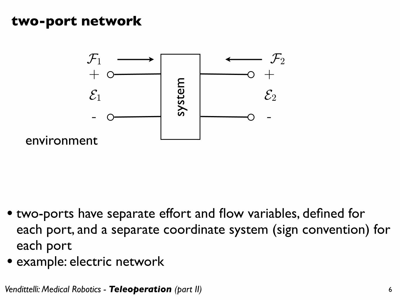
two-port network
+
-
F2
E2
syst
em
environment
• two-ports have separate effort and flow variables, defined for each port, and a separate coordinate system (sign convention) for each port
• example: electric network
F1
+
-
E1

Vendittelli: Medical Robotics - Teleoperation (part II) 7
two-port model of teleoperator
master +
comm. channel+
slave
Zh
—
+
Fh
—
+
Fh*
Ze
—
+
Fe
—
+
Fe*
Zt
Vh Ve
Fh*, Fe* exogenous force inputs generated by the operator and the environment respectively and Zt the transmitted impedance (i.e., seen by the human); here we assume Fe*=0
• bilateral teleoperation systems can be viewed as a cascade interconnection of two-port (master, communication channel and slave) and one-port (operator and environment) blocks
• using mechanical/electrical analogy and network theory, the teleoperation system is described as interconnection of one and two-port electrical elements

Vendittelli: Medical Robotics - Teleoperation (part II) 8
• in the two-port model the behavior of the system is completely characterized by measurements of the forces and velocities at the two ports
Fe = Ze Ve Fh = Zt Vh
• of these four involved variables, two may be chosen as independent and the remaining two dependent
• dependent variables are related to independent ones through the
• impedance (Fh,Fe,t)=Z(Vh,Ve,t)
• elements of Z can be found through experiments
• admittance (Vh,Ve,t)=Y(Fh,Fe,t)
• hybrid (Fh,Ve,t)=H(Vh,Fe,t)
• scattering (F-bV,t)=S(F+bV,t)
operators (transfer matrices for LTI systems)

Vendittelli: Medical Robotics - Teleoperation (part II) 9
for the same forces Fe = Fh we want the same motion Ve = Vh
transparency condition Zt = Ze
• what degree of transparency is possible?• what are suitable teleoperator architecture and control laws
for achieving necessary or optimal transparency?
transparency
for the analysis consider the linearized behavior around contact-operating point using the hybrid matrix formulationZ�1
s1Zs
Z�1m
�Fh(s)Vh(s)
⇥=
�H11(s) H12(s)H21(s) H22(s)
⇥ �Ve
�Fe
⇥
M. Vendittelli Medical Robotics (Universita di Roma “La Sapienza”) – Teleoperation 19
Fh = (H11-H12 Ze) (H21-H22 Ze)—1 Vh

Vendittelli: Medical Robotics - Teleoperation (part II) 10
a general architecture
+++
Ze
Zh
Z�1s
1Zs
M. Vendittelli Medical Robotics (Universita di Roma “La Sapienza”) – Teleoperation 19
Cs
VeFe
Fe*=0
Fsc
+
+—
C1C4 C3 C2
Cm
VhFh
Fh*
—
Z�1s
1Zs
Z�1m
M. Vendittelli Medical Robotics (Universita di Roma “La Sapienza”) – Teleoperation 19
——
—
Fmc
+
+
—
+
environment
slave
communicationchannel
master
humanoperator
Zt
master controller
slave controller
channelcontrollers
Vendittelli: Medical Robotics - Teleoperation (part II) 11
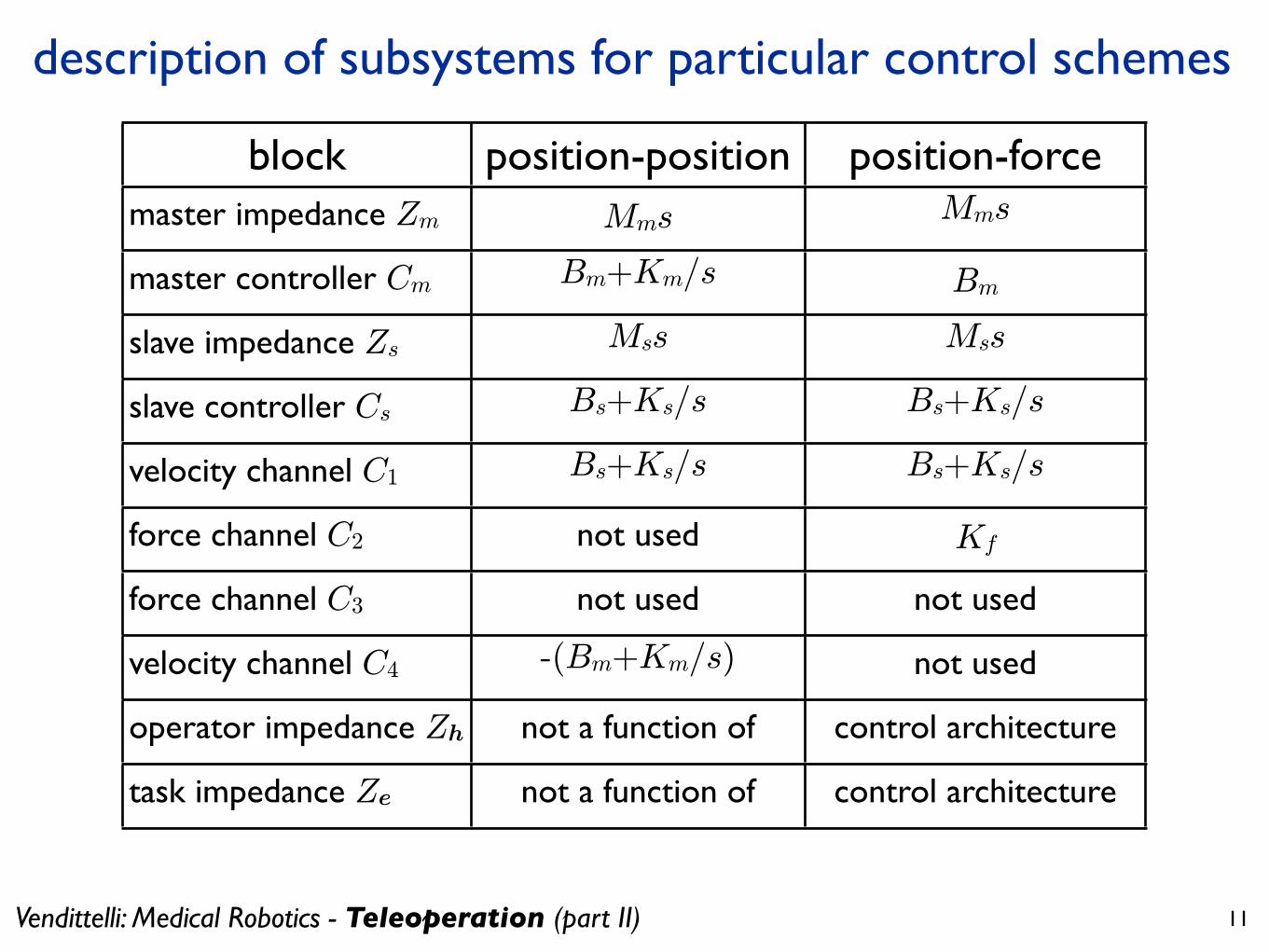
block position-position position-forcemaster impedance Zm Mms Mms
master controller Cm Bm+Km/s Bm
slave impedance Zs Mss Mss
slave controller Cs Bs+Ks/s Bs+Ks/s
velocity channel C1 Bs+Ks/s Bs+Ks/s
force channel C2 not used Kf
force channel C3 not used not used
velocity channel C4 -(Bm+Km/s) not used
operator impedance Zh not a function of control architecture
task impedance Ze not a function of control architecture
description of subsystems for particular control schemes

Vendittelli: Medical Robotics - Teleoperation (part II) 12
• solving for the transfer functions between master and slave forces and velocities
H11=(Zm + Cm)D(Zs + Cs — C3C4) + C4
H12= —(Zm + Cm)D(I — C3C2) — C2
H21= D(Zs + Cs — C3C4) — C2
H22= —D(I — C3C2)
D= (C1 + C3Zm + C3Cm)—1
• these expressions can be used to
• design suitable control laws Ci (i=1,..., 4, m, s)
• design suitable master and slave (Zm, Zs)
• compare transparency performance of different teleoperation architectures
• improve or optimize transparency

Vendittelli: Medical Robotics - Teleoperation (part II) 13
optimizing for transparency
• being Zt = (H11-H12 Ze) (H21-H22 Ze)—1
• perfect transparency (Zt=Ze) can be obtained by choosing Ci
(i=1,..., 4) s.t. H22=0, H11=0, H12=I:
• C3C2=I, C4=—(Zm + Cm), C1=(Zs + Cs), C2=I (C2≠I for telefunctioning) () a true 4-channel architecture)
• but C4=—(Zm + Cm), C1=(Zs + Cs) require acceleration measurements
• at low frequencies good transparency can be achieved with position and velocity measurements
• in any case, stability is an issue
Vendittelli: Medical Robotics - Teleoperation (part II) 14
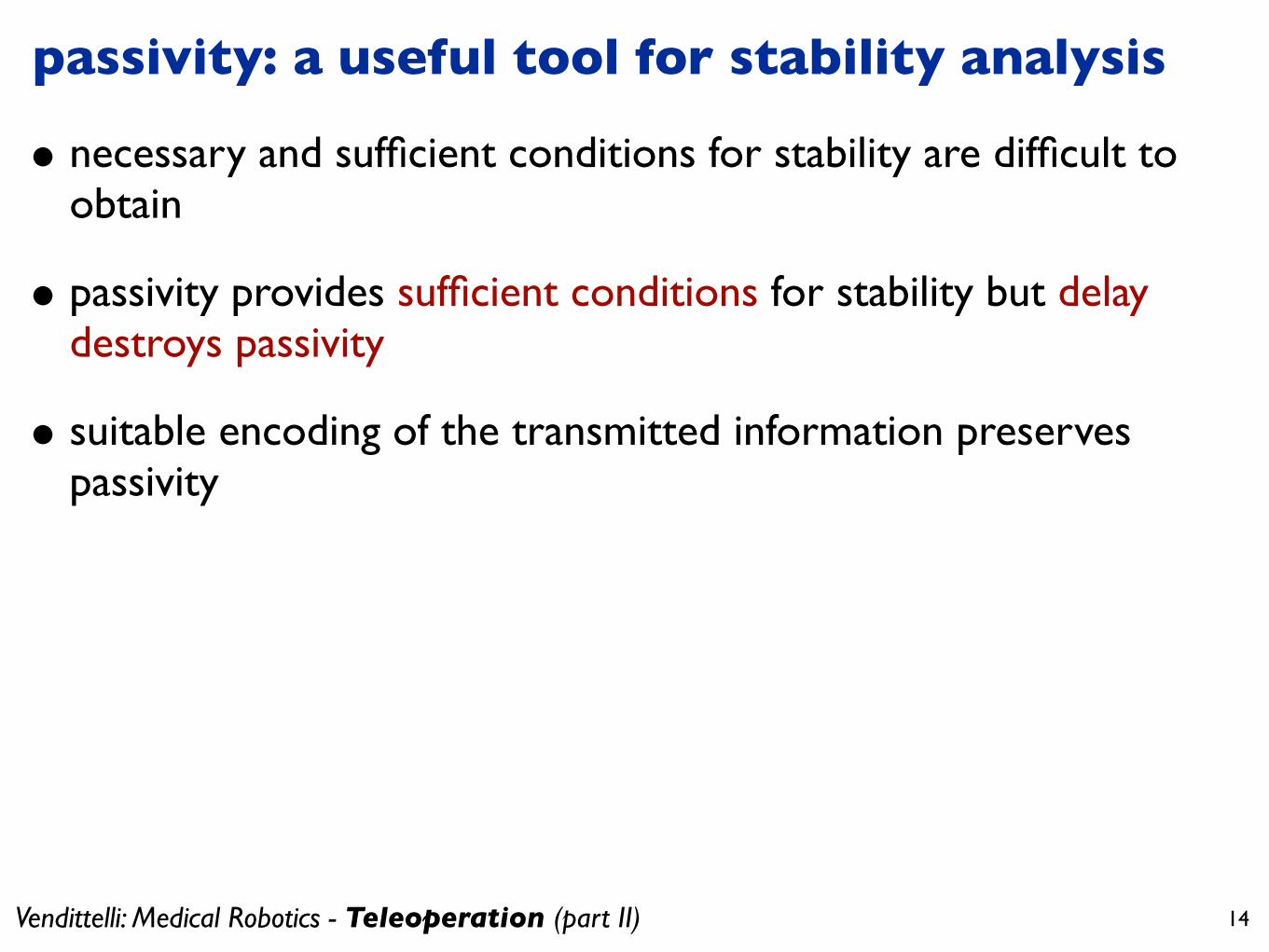
passivity: a useful tool for stability analysis
• necessary and sufficient conditions for stability are difficult to obtain
• passivity provides sufficient conditions for stability but delay destroys passivity
• suitable encoding of the transmitted information preserves passivity

Vendittelli: Medical Robotics - Teleoperation (part II) 15
definitionsconsider the state space description of a dynamic system
and assume f(0)=0 and h(0)=0the system is dissipative if there exist• a continuous lower bounded function of the state (storage
function)
•a function of the input/output pair (supply rate)
such that (equivalently)
u = [uTh uT
e ]T v = [vTh vT
e ]T
uh = 1⇥2b
(Fh + bVh) ue = 1⇥2b
(Fe � bVe)
vh = 1⇥2b
(Fh � bVh) ve = 1⇥2b
(Fe + bVe)
12
�vT vdt ⇥ 1
2
�uT udt
v(t) = S(t)u(t)⌅ F (t)� bV (t) = S(t)[F (t) + bV (t)]
v(s) = S(s)u(s)⌅ F (s)� bV (s) = S(s)[F (s) + bV (s)]
||s(s)|| ⇥ 1
||S(s)|| = sup� �1/2max{S�(j⇥)S(j⇥)} ⇥ 1
x = f(x) + g(x)y = h(x) x ⇧ Rn, u ⇧ Rm, y ⇧ Rm
V (x) ⇧ C1 : Rn ⇤ R+
1
u = [uTh uT
e ]T v = [vTh vT
e ]T
uh = 1⇥2b
(Fh + bVh) ue = 1⇥2b
(Fe � bVe)
vh = 1⇥2b
(Fh � bVh) ve = 1⇥2b
(Fe + bVe)
12
�vT vdt ⇤ 1
2
�uT udt
v(t) = S(t)u(t)⇧ F (t)� bV (t) = S(t)[F (t) + bV (t)]
v(s) = S(s)u(s)⇧ F (s)� bV (s) = S(s)[F (s) + bV (s)]
||s(s)|| ⇤ 1
||S(s)|| = sup� �1/2max{S�(j⇥)S(j⇥)} ⇤ 1
x = f(x) + g(x)y = h(x) x ⌃ Rn, u ⌃ Rm, y ⌃ Rm
V (x) ⌃ C1 : Rn ⌅ R+
w(u, y) : Rm ⇥Rm ⌅ R
1
u = [uTh uT
e ]T v = [vTh vT
e ]T
uh = 1⇥2b
(Fh + bVh) ue = 1⇥2b
(Fe � bVe)
vh = 1⇥2b
(Fh � bVh) ve = 1⇥2b
(Fe + bVe)
12
⇥vT vdt ⇤ 1
2
⇥uT udt
v(t) = S(t)u(t)⇧ F (t)� bV (t) = S(t)[F (t) + bV (t)]
v(s) = S(s)u(s)⇧ F (s)� bV (s) = S(s)[F (s) + bV (s)]
||S(s)|| ⇤ 1
||S(s)|| = sup� �1/2max{S�(j⇤)S(j⇤)} ⇤ 1
�x = f(x) + g(x)uy = h(x) x ⌃ Rn, u ⌃ Rm, y ⌃ Rm
x1 = f1(x1) + g1(x1)u1
y1 = h1(x1)
x2 = f2(x2) + g2(x2)u2
y2 = h2(x2)
V (x) ⌃ C1 : Rn ⌅ R+
w(u, y) : Rm ⇥Rm ⌅ R
V = V1 + V2 ⇤ yT1 v1 + yT
2 v2
V (x(t)) ⇤ V (x(t0)) +⇥ t
t0y(s)T u(s)ds
V (x(t)) ⇤ w(u(t)), y(t))
w(u, y) =< y, u >= yT u
V ⇤ 0
u = �⇥(y), yT ⇥(y) > 0�y ⌥= 0
u = �ky, k > 0
1
u = [uTh uT
e ]T v = [vTh vT
e ]T
uh = 1⇥2b
(Fh + bVh) ue = 1⇥2b
(Fe � bVe)
vh = 1⇥2b
(Fh � bVh) ve = 1⇥2b
(Fe + bVe)
12
⇧vT vdt ⇤ 1
2
⇧uT udt
v(t) = S(t)u(t)⇧ F (t)� bV (t) = S(t)[F (t) + bV (t)]
v(s) = S(s)u(s)⇧ F (s)� bV (s) = S(s)[F (s) + bV (s)]
||S(s)|| ⇤ 1
||S(s)|| = sup� �1/2max{S�(j⇥)S(j⇥)} ⇤ 1
�x = f(x) + g(x)uy = h(x) x ⌃ Rn, u ⌃ Rm, y ⌃ Rm
x1 = f1(x1) + g1(x1)u1
y1 = h1(x1)
x2 = f2(x2) + g2(x2)u2
y2 = h2(x2)
V (x) ⌃ C1 : Rn ⌅ R+
w(u, y) : Rm ⇥Rm ⌅ R
V = V1 + V2 ⇤ yT1 v1 + yT
2 v2
V (x(t)) ⇤ V (x(t0)) +⇧ t
t0y(s)T u(s)ds
V (x(t)) ⇤ w(u(t)), y(t))
⇥⌅
⇤
V (x(t))� V (x(t0)) ⇤⇧ t
t0w(u(s)), y(s))ds
V (x(t)) ⇤ w(u(t)), y(t))
w(u, y) =< y, u >= yT u
V ⇤ 0
1

Vendittelli: Medical Robotics - Teleoperation (part II) 16
when the supply rate is the scalar product between the in/out pair
dissipativity is named passivity and the system is said passive
V(x(t)) can be interpreted as the energy of the system: physically, a passive system cannot produce energy
current energy is at most equal to the initial energy + supplied energy from outside
u = [uTh uT
e ]T v = [vTh vT
e ]T
uh = 1⇥2b
(Fh + bVh) ue = 1⇥2b
(Fe � bVe)
vh = 1⇥2b
(Fh � bVh) ve = 1⇥2b
(Fe + bVe)
12
�vT vdt ⇤ 1
2
�uT udt
v(t) = S(t)u(t)⇧ F (t)� bV (t) = S(t)[F (t) + bV (t)]
v(s) = S(s)u(s)⇧ F (s)� bV (s) = S(s)[F (s) + bV (s)]
||s(s)|| ⇤ 1
||S(s)|| = sup� �1/2max{S�(j⇥)S(j⇥)} ⇤ 1
x = f(x) + g(x)y = h(x) x ⌃ Rn, u ⌃ Rm, y ⌃ Rm
V (x) ⌃ C1 : Rn ⌅ R+
w(u, y) : Rm ⇥Rm ⌅ R
V (x(t))� V (x(t0)) ⇤� t
t0w(u(s)), y(s))ds
V (x(t)) ⇤ w(u(t)), y(t))
w(u, y) =< y, u >= yT u
1
u = [uTh uT
e ]T v = [vTh vT
e ]T
uh = 1⇥2b
(Fh + bVh) ue = 1⇥2b
(Fe � bVe)
vh = 1⇥2b
(Fh � bVh) ve = 1⇥2b
(Fe + bVe)
12
�vT vdt ⇤ 1
2
�uT udt
v(t) = S(t)u(t)⇧ F (t)� bV (t) = S(t)[F (t) + bV (t)]
v(s) = S(s)u(s)⇧ F (s)� bV (s) = S(s)[F (s) + bV (s)]
||s(s)|| ⇤ 1
||S(s)|| = sup� �1/2max{S�(j⇥)S(j⇥)} ⇤ 1
x = f(x) + g(x)y = h(x) x ⌃ Rn, u ⌃ Rm, y ⌃ Rm
V (x) ⌃ C1 : Rn ⌅ R+
w(u, y) : Rm ⇥Rm ⌅ R
V (x(t)) ⇤ V (x(t0)) +� t
t0y(s)T u(s)ds
V (x(t)) ⇤ w(u(t)), y(t))
w(u, y) =< y, u >= yT u
1

Vendittelli: Medical Robotics - Teleoperation (part II) 17
link to Lyapunov stability•assume V(0)=0, i.e., 0 is a (local) minimum of the storage
function
•then V(x) is a Lyapunov candidate around 0 and
• if u´0 then i.e., 0 is a (Lyapunov) stable equilibrium (passivity ) stability of the unforced equilibrium)
• if y´0 then i.e., the zero dynamics of the system is (Lyapunov) stable
• the system can be stabilized by a static output feedback
• for instance
u = [uTh uT
e ]T v = [vTh vT
e ]T
uh = 1⇥2b
(Fh + bVh) ue = 1⇥2b
(Fe � bVe)
vh = 1⇥2b
(Fh � bVh) ve = 1⇥2b
(Fe + bVe)
12
�vT vdt ⇤ 1
2
�uT udt
v(t) = S(t)u(t)⇧ F (t)� bV (t) = S(t)[F (t) + bV (t)]
v(s) = S(s)u(s)⇧ F (s)� bV (s) = S(s)[F (s) + bV (s)]
||s(s)|| ⇤ 1
||S(s)|| = sup� �1/2max{S�(j⇤)S(j⇤)} ⇤ 1
x = f(x) + g(x)y = h(x) x ⌃ Rn, u ⌃ Rm, y ⌃ Rm
V (x) ⌃ C1 : Rn ⌅ R+
w(u, y) : Rm ⇥Rm ⌅ R
V (x(t)) ⇤ V (x(t0)) +� t
t0y(s)T u(s)ds
V (x(t)) ⇤ w(u(t)), y(t))
w(u, y) =< y, u >= yT u
V ⇤ 0
u = �⇥(y), yT ⇥(y) > 0�y ⌥= 0
1
u = [uTh uT
e ]T v = [vTh vT
e ]T
uh = 1⇥2b
(Fh + bVh) ue = 1⇥2b
(Fe � bVe)
vh = 1⇥2b
(Fh � bVh) ve = 1⇥2b
(Fe + bVe)
12
�vT vdt ⇤ 1
2
�uT udt
v(t) = S(t)u(t)⇧ F (t)� bV (t) = S(t)[F (t) + bV (t)]
v(s) = S(s)u(s)⇧ F (s)� bV (s) = S(s)[F (s) + bV (s)]
||s(s)|| ⇤ 1
||S(s)|| = sup� �1/2max{S�(j⇤)S(j⇤)} ⇤ 1
x = f(x) + g(x)y = h(x) x ⌃ Rn, u ⌃ Rm, y ⌃ Rm
V (x) ⌃ C1 : Rn ⌅ R+
w(u, y) : Rm ⇥Rm ⌅ R
V (x(t)) ⇤ V (x(t0)) +� t
t0y(s)T u(s)ds
V (x(t)) ⇤ w(u(t)), y(t))
w(u, y) =< y, u >= yT u
V ⇤ 0
u = �⇥(y), yT ⇥(y) > 0�y ⌥= 0
u = �ky, k > 0
1
) can be used to establish stability or to design a stabilizing feedback

Vendittelli: Medical Robotics - Teleoperation (part II) 18
feedback interconnection• given two passive systems with appropriate in/out dimensions and
storage functions V1(x1) and V2(x2)
• their feedback interconnection is passive w.r.t. V1(x1)+ V2(x2) with (new) input v=(v1, v2) and output y=(y1, y2) pairs
• it easily follows from
u = [uTh uT
e ]T v = [vTh vT
e ]T
uh = 1⇥2b
(Fh + bVh) ue = 1⇥2b
(Fe � bVe)
vh = 1⇥2b
(Fh � bVh) ve = 1⇥2b
(Fe + bVe)
12
�vT vdt ⇤ 1
2
�uT udt
v(t) = S(t)u(t)⇧ F (t)� bV (t) = S(t)[F (t) + bV (t)]
v(s) = S(s)u(s)⇧ F (s)� bV (s) = S(s)[F (s) + bV (s)]
||s(s)|| ⇤ 1
||S(s)|| = sup� �1/2max{S�(j⇤)S(j⇤)} ⇤ 1
x = f(x) + g(x)uy = h(x) x ⌃ Rn, u ⌃ Rm, y ⌃ Rm
x1 = f1(x1) + g1(x1)u1
y1 = h1(x1)
x2 = f2(x2) + g2(x2)u2
y2 = h2(x2)
V (x) ⌃ C1 : Rn ⌅ R+
w(u, y) : Rm ⇥Rm ⌅ R
V = V1 + V2 ⇤ yT1 v1 + yT
2 v2
V (x(t)) ⇤ V (x(t0)) +� t
t0y(s)T u(s)ds
V (x(t)) ⇤ w(u(t)), y(t))
w(u, y) =< y, u >= yT u
V ⇤ 0
u = �⇥(y), yT ⇥(y) > 0�y ⌥= 0
u = �ky, k > 0
1
u = [uTh uT
e ]T v = [vTh vT
e ]T
uh = 1⇥2b
(Fh + bVh) ue = 1⇥2b
(Fe � bVe)
vh = 1⇥2b
(Fh � bVh) ve = 1⇥2b
(Fe + bVe)
12
⇧vT vdt ⇤ 1
2
⇧uT udt
v(t) = S(t)u(t)⇧ F (t)� bV (t) = S(t)[F (t) + bV (t)]
v(s) = S(s)u(s)⇧ F (s)� bV (s) = S(s)[F (s) + bV (s)]
||S(s)|| ⇤ 1
||S(s)|| = sup� �1/2max{S�(j⇥)S(j⇥)} ⇤ 1
�x = f(x) + g(x)uy = h(x) x ⌃ Rn, u ⌃ Rm, y ⌃ Rm
�x1 = f1(x1) + g1(x1)u1
y1 = h1(x1)
�x2 = f2(x2) + g2(x2)u2
y2 = h2(x2)
V (x) ⌃ C1 : Rn ⌅ R+
w(u, y) : Rm ⇥Rm ⌅ R
V = V1 + V2 ⇤ yT1 v1 + yT
2 v2
V (x(t)) ⇤ V (x(t0)) +⇧ t
t0y(s)T u(s)ds
V (x(t)) ⇤ w(u(t)), y(t))
⇥⌅
⇤
V (x(t))� V (x(t0)) ⇤⇧ t
t0w(u(s)), y(s))ds
V (x(t)) ⇤ w(u(t)), y(t))
w(u, y) =< y, u >= yT u
V ⇤ 0
1
u = [uTh uT
e ]T v = [vTh vT
e ]T
uh = 1⇥2b
(Fh + bVh) ue = 1⇥2b
(Fe � bVe)
vh = 1⇥2b
(Fh � bVh) ve = 1⇥2b
(Fe + bVe)
12
⇧vT vdt ⌅ 1
2
⇧uT udt
v(t) = S(t)u(t)⌃ F (t)� bV (t) = S(t)[F (t) + bV (t)]
v(s) = S(s)u(s)⌃ F (s)� bV (s) = S(s)[F (s) + bV (s)]
||S(s)|| ⌅ 1
||S(s)|| = sup� �1/2max{S�(j⇥)S(j⇥)} ⌅ 1
�x = f(x) + g(x)uy = h(x) x ⌥ Rn, u ⌥ Rm, y ⌥ Rm
�x1 = f1(x1) + g1(x1)u1
y1 = h1(x1)
�x2 = f2(x2) + g2(x2)u2
y2 = h2(x2)
�u1 = ± y2 + v1
u2 = ⇤ y1 + v2
V (x) ⌥ C1 : Rn ⇧ R+
w(u, y) : Rm ⇥Rm ⇧ R
V = V1 + V2 ⌅ yT1 v1 + yT
2 v2
V (x(t)) ⌅ V (x(t0)) +⇧ t
t0y(s)T u(s)ds
V (x(t)) ⌅ w(u(t)), y(t))
⇥⌅
⇤
V (x(t))� V (x(t0)) ⌅⇧ t
t0w(u(s)), y(s))ds
V (x(t)) ⌅ w(u(t)), y(t))
1

Vendittelli: Medical Robotics - Teleoperation (part II) 19
scattering representation: wave variablesconsider the total power flow P in a two-port element as composed of two terms: the input power Pin and output power Pout; denote the effort F=[Fh Fe]T and the flow V=[Vh -Ve]T
P = Pin – Pout = F T V = FhVh – FeVe = 1/2(uTu – vTv)
with
NOTE: a scaling factor b is assumed between forces and velocities
u = [uTh uT
e ]T v = [vTh vT
e ]T
uh = 1�2b
(Fh + bVh) ue = 1�2b
(Fe � bVe)
vh = 1�2b
(Fh � bVh) ve = 1�2b
(Fe + bVe)
1
S
uh ue
vh ve
Vendittelli: Medical Robotics - Teleoperation (part II) 20
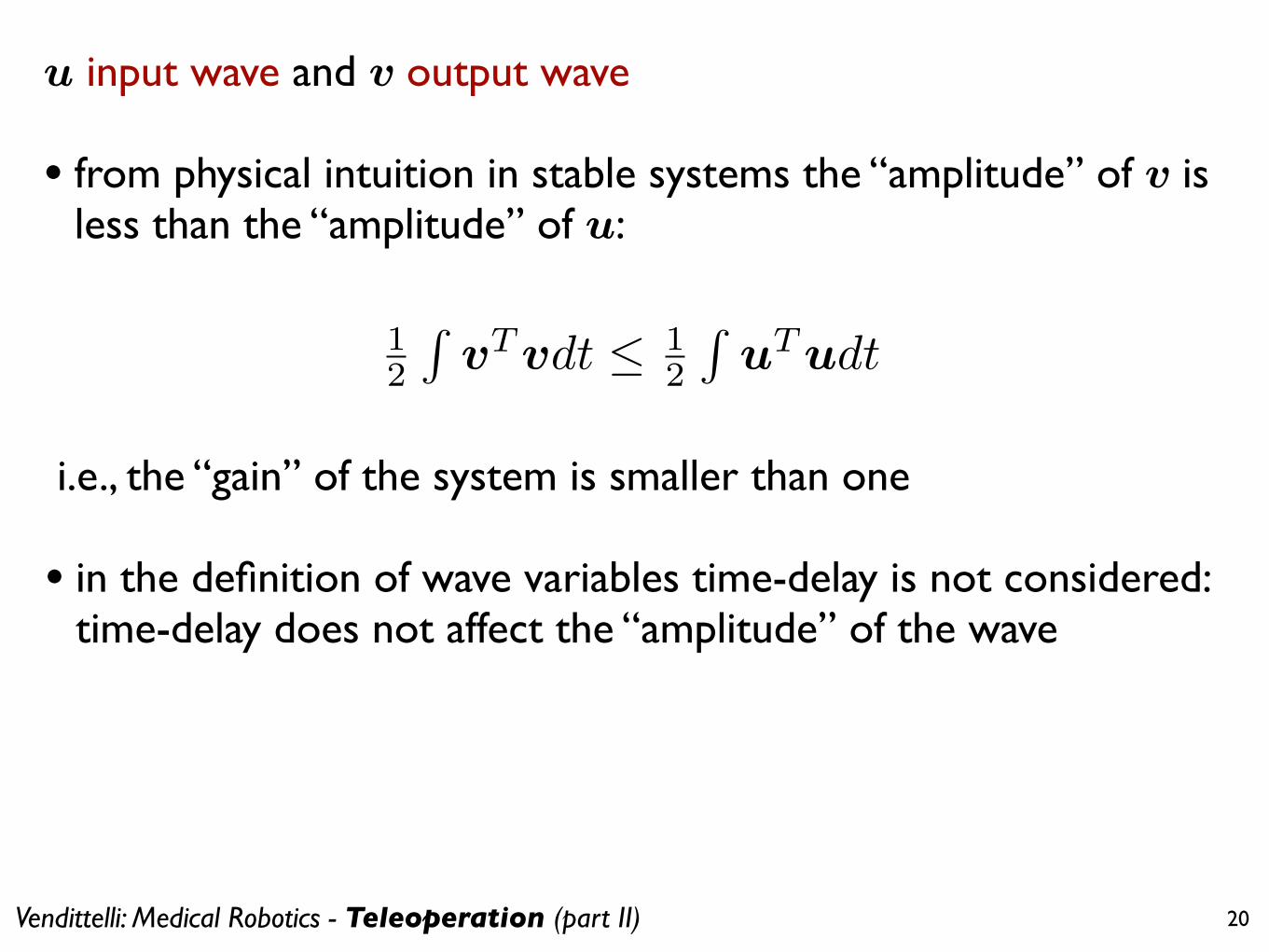
u input wave and v output wave
• from physical intuition in stable systems the “amplitude” of v is less than the “amplitude” of u:
i.e., the “gain” of the system is smaller than one
• in the definition of wave variables time-delay is not considered: time-delay does not affect the “amplitude” of the wave
u = [uTh uT
e ]T v = [vTh vT
e ]T
uh = 1�2b
(Fh + bVh) ue = 1�2b
(Fe � bVe)
vh = 1�2b
(Fh � bVh) ve = 1�2b
(Fe + bVe)
12
�vT vdt ⇥ 1
2
�uT udt
1

Vendittelli: Medical Robotics - Teleoperation (part II) 21
• the scattering operator (or matrix) relates the input/output wave variables, u and v, at each port of the teleoperator instead of the power variables (velocities and forces)
• given an n-port system, the scattering matrix (or scattering operator) is defined as the operator which relates input and output wave variables as:
for LTI systems
u = [uTh uT
e ]T v = [vTh vT
e ]T
uh = 1�2b
(Fh + bVh) ue = 1�2b
(Fe � bVe)
vh = 1�2b
(Fh � bVh) ve = 1�2b
(Fe + bVe)
12
�vT vdt ⇥ 1
2
�uT udt
v(t) = S(t)u(t)⇤ F (t)� bV (t) = S(t)[F (t) + bV (t)]
1
u = [uTh uT
e ]T v = [vTh vT
e ]T
uh = 1�2b
(Fh + bVh) ue = 1�2b
(Fe � bVe)
vh = 1�2b
(Fh � bVh) ve = 1�2b
(Fe + bVe)
12
�vT vdt ⇥ 1
2
�uT udt
v(t) = S(t)u(t)⇤ F (t)� bV (t) = S(t)[F (t) + bV (t)]
v(s) = S(s)u(s)⇤ F (s)� bV (s) = S(s)[F (s) + bV (s)]
1
• if the power variables are related by the hybrid matrix H(s):
• scattering and hybrid representation are related by
S(s) =
I 00 �I
�[H(s)� I][H(s) + I]�1
Fh(s)
�Ve(s)
�= H(s)
Vh(s)
Fe(s)
�
dim(C) = nq
t 2 T , dim(T ) = nt
T =
m
cos(#) cos(')
[g �Kzp(zd � z)�Kzd(zd � z)]
xd(t) = cos t
yd(t) = sin t
zd(t) = 1 +
t
10
� = T (⇠, ⇣)
⇠ 2 R
n, u 2 R
m
⌘ = h(⇠)
⌘
(r)= l(⇠, ⇣) + J(⇠, ⇣)u
u = J(⇠, ⇣)
�1(�l(⇠, ⇣) + v)
x
(4)= ⌘
(4)1 = v1
y
(4)= ⌘
(4)2 = v2
z
(4)= ⌘
(4)3 = v3
(2)= ⌘
(2)4 = v4
v1 = ⌘
(4)1d +
P4j=1 c
1j�1e
(j�1)1
v2 = ⌘
(4)2d +
P4j=1 c
2j�1e
(j�1)2
v3 = ⌘
(4)3d +
P4j=1 c
3j�1e
(j�1)3
v4 = ⌘
(2)4d +
P2j=1 c
4j�1e
(j�1)4
˙
T
¨
T
˙
⇣ = a(⇠, ⇣) + b(⇠, ⇣)v
u = c(⇠, ⇣) + d(⇠, ⇣)v
1

Vendittelli: Medical Robotics - Teleoperation (part II) 22
scattering vs passivitytheorem an LTI n-port element with scattering matrix S(s) is passive if and only if
corollary an LTI n-port element with scattering matrix S(s) is passive if and only if
where ¸max {S(j!)} is the maximum eigenvalue and S*(j!) the transpose conjugate of S(j!)
u = [uTh uT
e ]T v = [vTh vT
e ]T
uh = 1⇥2b
(Fh + bVh) ue = 1⇥2b
(Fe � bVe)
vh = 1⇥2b
(Fh � bVh) ve = 1⇥2b
(Fe + bVe)
12
�vT vdt ⇤ 1
2
�uT udt
v(t) = S(t)u(t)⇧ F (t)� bV (t) = S(t)[F (t) + bV (t)]
v(s) = S(s)u(s)⇧ F (s)� bV (s) = S(s)[F (s) + bV (s)]
||s(s)|| ⇤ 1
||S(s)|| = sup� �1/2max{S�(j⇤)S(j⇤)} ⇤ 1
x = f(x) + g(x)uy = h(x) x ⌃ Rn, u ⌃ Rm, y ⌃ Rm
x1 = f1(x1) + g1(x1)u1
y1 = h1(x1)
x2 = f2(x2) + g2(x2)u2
y2 = h2(x2)
V (x) ⌃ C1 : Rn ⌅ R+
w(u, y) : Rm ⇥Rm ⌅ R
V = V1 + V2 ⇤ yT1 v1 + yT
2 v2
V (x(t)) ⇤ V (x(t0)) +� t
t0y(s)T u(s)ds
V (x(t)) ⇤ w(u(t)), y(t))
w(u, y) =< y, u >= yT u
V ⇤ 0
u = �⇥(y), yT ⇥(y) > 0�y ⌥= 0
u = �ky, k > 0
1
u = [uTh uT
e ]T v = [vTh vT
e ]T
uh = 1⇥2b
(Fh + bVh) ue = 1⇥2b
(Fe � bVe)
vh = 1⇥2b
(Fh � bVh) ve = 1⇥2b
(Fe + bVe)
12
�vT vdt ⇤ 1
2
�uT udt
v(t) = S(t)u(t)⇧ F (t)� bV (t) = S(t)[F (t) + bV (t)]
v(s) = S(s)u(s)⇧ F (s)� bV (s) = S(s)[F (s) + bV (s)]
||S(s)|| ⇤ 1
||S(s)|| = sup� �1/2max{S�(j⇤)S(j⇤)} ⇤ 1
x = f(x) + g(x)uy = h(x) x ⌃ Rn, u ⌃ Rm, y ⌃ Rm
x1 = f1(x1) + g1(x1)u1
y1 = h1(x1)
x2 = f2(x2) + g2(x2)u2
y2 = h2(x2)
V (x) ⌃ C1 : Rn ⌅ R+
w(u, y) : Rm ⇥Rm ⌅ R
V = V1 + V2 ⇤ yT1 v1 + yT
2 v2
V (x(t)) ⇤ V (x(t0)) +� t
t0y(s)T u(s)ds
V (x(t)) ⇤ w(u(t)), y(t))
w(u, y) =< y, u >= yT u
V ⇤ 0
u = �⇥(y), yT ⇥(y) > 0�y ⌥= 0
u = �ky, k > 0
1
proof see reference 3. in the bibliography

Vendittelli: Medical Robotics - Teleoperation (part II) 23
• connection of passive n-port preserves passivity
• in traditional force reflection schemes, time-delay instabilities are originated by the non-passive features of the communication line
• the use of a particular communication channel based on the analogous of a lossless transmission line results in a passive communication channel (Passivity Based Teleoperation)
Vendittelli: Medical Robotics - Teleoperation (part II) 24
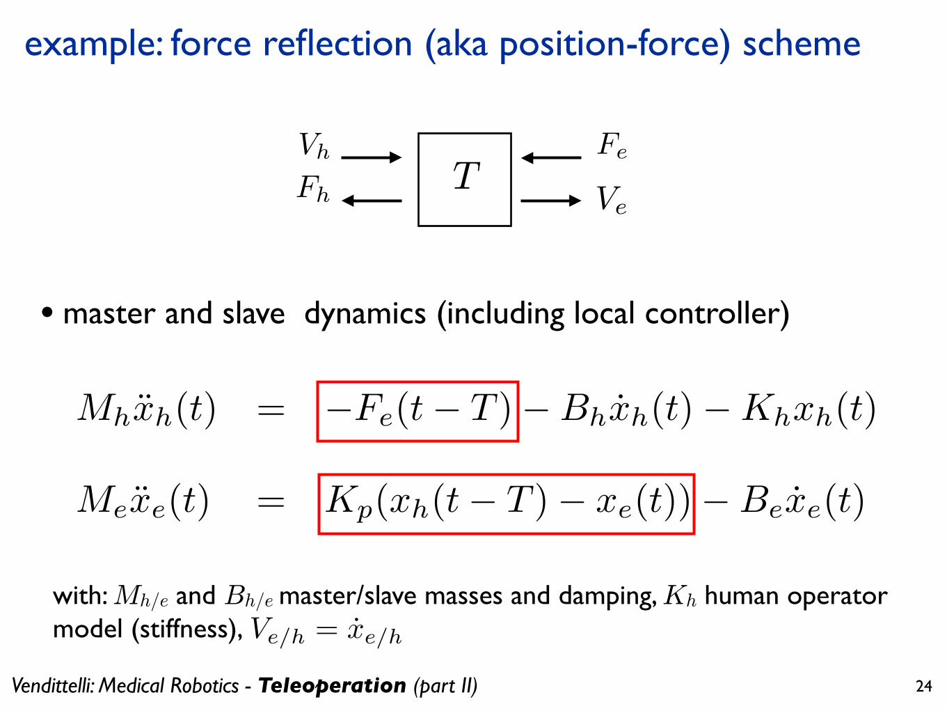
example: force reflection (aka position-force) scheme
T
u = [uTh uT
e ]T v = [vTh vT
e ]T
uh = 1⇥2b
(Fh + bVh) ue = 1⇥2b
(Fe � bVe)
vh = 1⇥2b
(Fh � bVh) ve = 1⇥2b
(Fe + bVe)
12
⇧vT vdt ⌅ 1
2
⇧uT udt
v(t) = S(t)u(t)⌃ F (t)� bV (t) = S(t)[F (t) + bV (t)]
v(s) = S(s)u(s)⌃ F (s)� bV (s) = S(s)[F (s) + bV (s)]
||S(s)|| ⌅ 1
||S(s)|| = sup� �1/2max{S�(j⇥)S(j⇥)} ⌅ 1
�x = f(x) + g(x)uy = h(x) x ⌥ Rn, u ⌥ Rm, y ⌥ Rm
�x1 = f1(x1) + g1(x1)u1
y1 = h1(x1)
�x2 = f2(x2) + g2(x2)u2
y2 = h2(x2)
�u1 = ± y2 + v1
u2 = ⇤ y1 + v2
V (x) ⌥ C1 : Rn ⇧ R+
w(u, y) : Rm ⇥Rm ⇧ R
V = V1 + V2 ⌅ yT1 v1 + yT
2 v2
V (x(t)) ⌅ V (x(t0)) +⇧ t
t0y(s)T u(s)ds
V (x(t)) ⌅ w(u(t)), y(t))
⇥⌅
⇤
V (x(t))� V (x(t0)) ⌅⇧ t
t0w(u(s)), y(s))ds
V (x(t)) ⌅ w(u(t)), y(t))
1
• master and slave dynamics (including local controller)
w(u, y) =< y, u >= yT u
V ⇥ 0
u = ��(y), yT �(y) > 0⌅y ⇤= 0
u = �ky, k > 0
Mhxh(t) = �Fe(t� T )�Bhxh(t)�Khxh(t)
Mexe(t) = Kp(xh(t� T )� xe(t))�Bexe(t)
2
with: Mh/e and Bh/e master/slave masses and damping, Kh human operator model (stiffness),
w(u, y) =< y, u >= yT u
V ⇥ 0
u = ��(y), yT �(y) > 0⌅y ⇤= 0
u = �ky, k > 0
Mhxh(t) = �Fe(t� T )�Bhxh(t)�Khxh(t)
Mexe(t) = Kp(xh(t� T )� xe(t))�Bexe(t)
Ve/h = xe/h
2

Vendittelli: Medical Robotics - Teleoperation (part II) 25
using the two-port model, relationships between forces and velocities can be expressed as
Fh = e-sTFe
Ve = e-sT Vh
with scattering matrix computed in s=j!
w(u, y) =< y, u >= yT u
V ⇥ 0
u = ��(y), yT �(y) > 0⌅y ⇤= 0
u = �ky, k > 0
Mhxh(t) = �Fe(t� T )�Bhxh(t)�Khxh(t)
Mexe(t) = Kp(xh(t� T )� xe(t))�Bexe(t)
Ve/h = xe/h
S(j⇥) =
�
⇤�j tan(⇥T ) sec(⇥T )
sec(⇥T ) j tan(⇥T )
⇥
⌅
2
the norm of the scattering matrix kS(j!)k=sup!{|tan(!T)| + |sec(!T)|}
is infinite and passivity conditions are not verified even for small T
• the introduction of a force gain reduces the performance and does not improve stability property
• in practical applications passivity can be achieved by introducing attenuation in the local controller

Vendittelli: Medical Robotics - Teleoperation (part II) 26
passivity based teleoperation
• standard methods for communicating forces and velocities cause instability in the presence of time delays
• idea: use a control law s.t. the two-port characteristics of the transmission block are identical to those of a lossless transmission line
Fhd(s) = tanh(sT)Vh + sech(sT)Fe(s)
-Ved(s) = -sech(sT)Vh + tanh(sT)Fe(s)
• resulting in the hybrid matrix
Vendittelli: Medical Robotics - Teleoperation (part II) 27
passivity based teleoperation
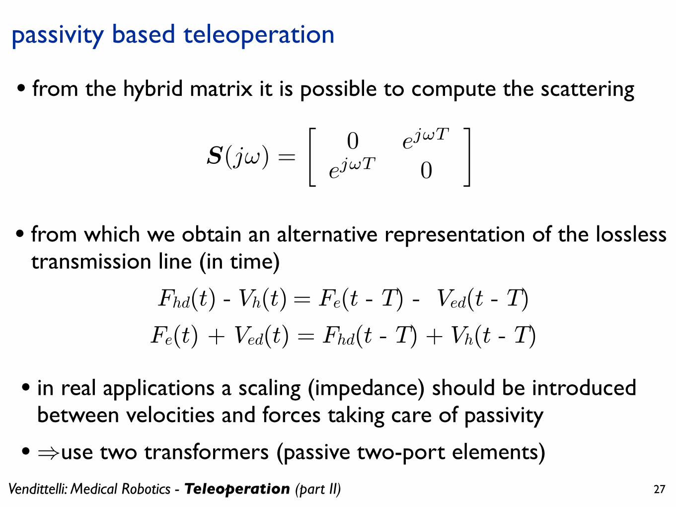
• from the hybrid matrix it is possible to compute the scattering
• from which we obtain an alternative representation of the lossless transmission line (in time)
Fhd(t) - Vh(t) = Fe(t - T) - Ved(t - T)
Fe(t) + Ved(t) = Fhd(t - T) + Vh(t - T)
• in real applications a scaling (impedance) should be introduced between velocities and forces taking care of passivity
•)use two transformers (passive two-port elements)
S(j!) =
0 e
j!T
e
j!T0
�[H(s)� I][H(s) + I]�1
Fh(s)
�Ve(s)
�= H(s)
Vh(s)
Fe(s)
�
dim(C) = nq
t 2 T , dim(T ) = nt
T =
m
cos(#) cos(')
[g �Kzp(zd � z)�Kzd(zd � z)]
xd(t) = cos t
yd(t) = sin t
zd(t) = 1 +
t
10
� = T (⇠, ⇣)
⇠ 2 R
n, u 2 R
m
⌘ = h(⇠)
⌘
(r)= l(⇠, ⇣) + J(⇠, ⇣)u
u = J(⇠, ⇣)
�1(�l(⇠, ⇣) + v)
x
(4)= ⌘
(4)1 = v1
y
(4)= ⌘
(4)2 = v2
z
(4)= ⌘
(4)3 = v3
(2)= ⌘
(2)4 = v4
v1 = ⌘
(4)1d +
P4j=1 c
1j�1e
(j�1)1
v2 = ⌘
(4)2d +
P4j=1 c
2j�1e
(j�1)2
v3 = ⌘
(4)3d +
P4j=1 c
3j�1e
(j�1)3
v4 = ⌘
(2)4d +
P2j=1 c
4j�1e
(j�1)4
˙
T
¨
T
˙
⇣ = a(⇠, ⇣) + b(⇠, ⇣)v
u = c(⇠, ⇣) + d(⇠, ⇣)v
1
Vendittelli: Medical Robotics - Teleoperation (part II) 28
passivity based teleoperation
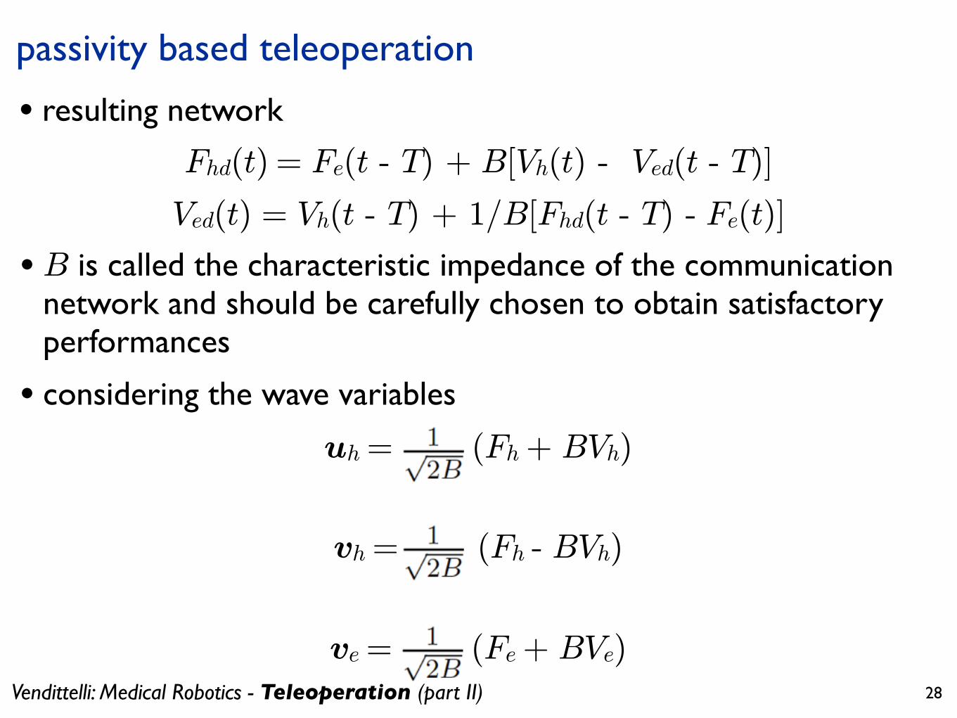
• resulting network
Fhd(t) = Fe(t - T) + B[Vh(t) - Ved(t - T)]
Ved(t) = Vh(t - T) + 1/B[Fhd(t - T) - Fe(t)]
• B is called the characteristic impedance of the communication network and should be carefully chosen to obtain satisfactory performances
• considering the wave variables
uh = (Fh + BVh)
vh = (Fh - BVh)
ve = (Fe + BVe)
Vendittelli: Medical Robotics - Teleoperation (part II) 29
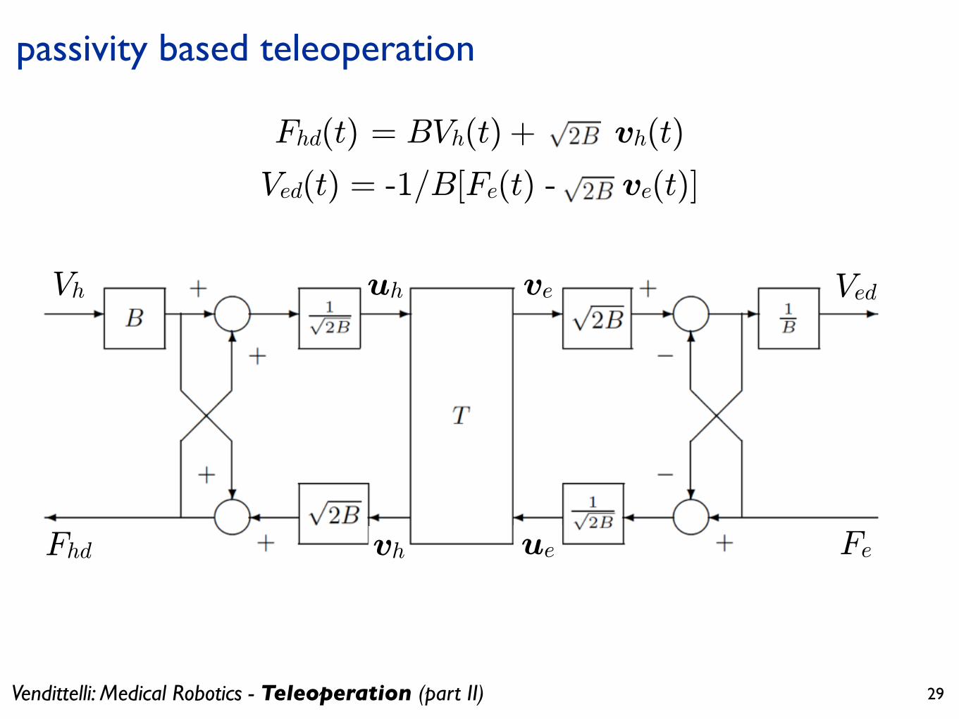
passivity based teleoperation
Fhd(t) = BVh(t) + vh(t)
Ved(t) = -1/B[Fe(t) - ve(t)]
Vh
Fhd
uh
vh
ve
ue
Ved
Fe

Vendittelli: Medical Robotics - Teleoperation (part II) 30
comments
• lossless TL provides non-strict passivity kS(j!)k=1
• impedance mismatches at the extremities of the communication line originate power reflections at both sites of the teleoperation system
• impedance adaptation at the termination by means of two admittance/impedance elements whose values are tuned with the characteristic impedance of the line
• compensation of the drift introduced by power modification due to impedance adaptation elements
Vendittelli: Medical Robotics - Teleoperation (part II) 31
bibliography
1.D. A. Lawrence, ‘‘Stability and transparency in bilateral teleoperation,’’ IEEE Trans. on Robotics and Automation, vol. 9, no. 5, pp. 624–637, 1993
2.B. Hannaford, ‘‘A design framework for teleoperators with kinesthetic feedback,’’ IEEE Trans. Robotics and Automation, vol. 5, no. 4, pp. 426–434, 1989
3.R. J. Anderson and M. W. Spong, “Bilateral control of teleoperators with time delay,” 27th Conference on Decision and Control, pp. 167–173, 1988
4.K. Hashtrudi-Zaad, Septimiu E. Salcudean, “Analysis of Control Architectures for Teleoperation Systems with Impedance/Admittance Master and Slave Manipulators,” IJRR, vol. 20, no. 6, pp. 419-445, 2001