stability analysis of cellular neural networks with nonlinear dynamics

Nonlinear Analysis: Real World Applications 2 (2001) 93–103www.elsevier.nl/locate/na

Stability analysis of cellular neural networkswith nonlinear dynamics

Angela Slavova 1

Institute of Mathematics, Bulgarian Academy of Sciences, So�a 1113, Bulgaria

Received 23 February 1995

Keywords: Cellular neural networks; Perturbed systems; Lyapunov’s majorizing equations;Integro-di�erential equations

1. Introduction

Cellular neural networks (CNNs), introduced by Chua and Yang [1], o�er a newapproach to real-time signal processing.

De�nition 1. The CNN is a(i) 2-, 3-, or n- dimensional array of(ii) mainly identical dynamical systems, called cells, which satis�es two

properties:(iii) most interactions are local within a �nite radius r, and(iv) all state variables are continuous valued signals.

In this paper we show that by retaining all important features of the original CNNstructure [1] and by introducing nonlinearity in the templates, the CNN becomes apowerful framework for general analogue array dynamics.

1 This paper is partially supported by Grant MM-706.

E-mail address: [email protected] (A. Slavova).

1468-1218/01/$ - see front matter ? 2001 Elsevier Science Ltd. All rights reserved.PII: S0362 -546X(00)00094 -8

94 A. Slavova / Nonlinear Analysis: Real World Applications 2 (2001) 93–103

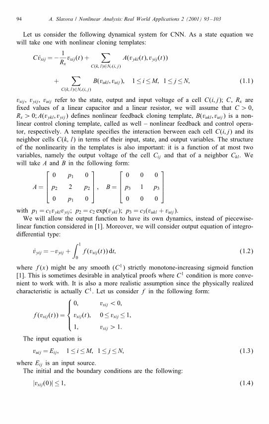
Let us consider the following dynamical system for CNN. As a state equation wewill take one with nonlinear cloning templates:

Cvxij =− 1Rx

vxij(t) +∑

C(k; l)∈Nr(i; j)

A(vykl(t); vyij(t))

+∑

C(k; l)∈Nr(i; j)

B(vukl; vuij); 1≤ i≤M; 1≤ j≤N; (1.1)

vxij, vyij, vuij refer to the state, output and input voltage of a cell C(i; j); C, Rx are�xed values of a linear capacitor and a linear resistor, we will assume that C ¿ 0,Rx ¿ 0;A(vykl; vyij) de�nes nonlinear feedback cloning template, B(vukl; vuij) is a non-linear control cloning template, called as well – nonlinear feedback and control opera-tor, respectively. A template speci�es the interaction berween each cell C(i; j) and itsneighbor cells C(k; l) in terms of their input, state, and output variables. The structureof the nonlinearity in the templates is also important: it is a function of at most twovariables, namely the output voltage of the cell Cij and that of a neighbor Ckl. Wewill take A and B in the following form:

A=

0 p1 0

p2 2 p2

0 p1 0

; B=

0 0 0

p3 1 p3

0 0 0

with p1 = c1vyklvyij; p2 = c2 exp(vykl); p3 = c3(vukl + vuij).We will allow the output function to have its own dynamics, instead of piecewise-

linear function considered in [1]. Moreover, we will consider output equation of integro-di�erential type:

vyij =−vyij +∫ 1

0f(vxij(t)) dt; (1.2)

where f(x) might be any smooth (C1) strictly monotone-increasing sigmoid function[1]. This is sometimes desirable in analytical proofs where C1 condition is more conve-nient to work with. It is also a more realistic assumption since the physically realizedcharacteristic is actually C1. Let us consider f in the following form:

f(vxij(t)) =

0; vxij ¡ 0;

vxij(t); 0≤ vxij ≤ 1;1; vxij ¿ 1:

The input equation is

vuij = Eij; 1≤ i≤M; 1≤ j≤N; (1.3)

where Eij is an input source.The initial and the boundary conditions are the following:

|vxij(0)| ≤ 1; (1.4)

A. Slavova / Nonlinear Analysis: Real World Applications 2 (2001) 93–103 95

|vuij| ≤ 1; (1.5)

|vyij(0)| ≤ 1: (1.6)

The proposed architecture of a CNN is quite general. The nonlinear cloning tem-plates allow us to model some biological problems, and also it can be used for model-ing motion dynamics. The output equation (1.2) gives more possibilities for complexdynamics and interesting phenomena. It is very useful for the circuit layout and thesoftware programmability of a CNN described above.In Section 2 of this paper we will de�ne dynamic range of a CNN and we will make

steady-state analysis. Section 3 deals with perturbed CNN [5]. The solutions for suchCNN are constructed by applying the method of Lyapunov’s majorizing equations. InSection 4 we will give some numerical results for this quite general CNN architecture.

2. Dynamic properties and stability

2.1. Dynamic range

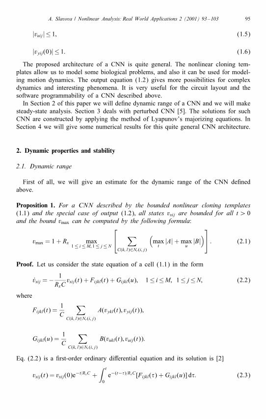
First of all, we will give an estimate for the dynamic range of the CNN de�nedabove.

Proposition 1. For a CNN described by the bounded nonlinear cloning templates(1:1) and the special case of output (1:2); all states vxij are bounded for all t ¿ 0and the bound vmax can be computed by the following formula:

vmax = 1 + Rx max1≤ i≤M; 1≤ j≤N

∑

C(k; l)∈Nr(i; j)

(max

t|A|+max

u|B|) : (2.1)

Proof. Let us consider the state equation of a cell (1.1) in the form

vxij =− 1RxC

vxij(t) + Fijkl(t) + Gijkl(u); 1≤ i≤M; 1≤ j≤N; (2.2)

where

Fijkl(t) =1C

∑C(k; l)∈Nr(i; j)

A(vykl(t); vyij(t));

Gijkl(u) =1C


B(vukl(t); vuij(t)):

Eq. (2.2) is a �rst-order ordinary di�erential equation and its solution is [2]

vxij(t) = vxij(0)e−t=RxC +∫ t

0e−(t−�)=RxC[Fijkl(�) + Gijkl(u)] d�: (2.3)


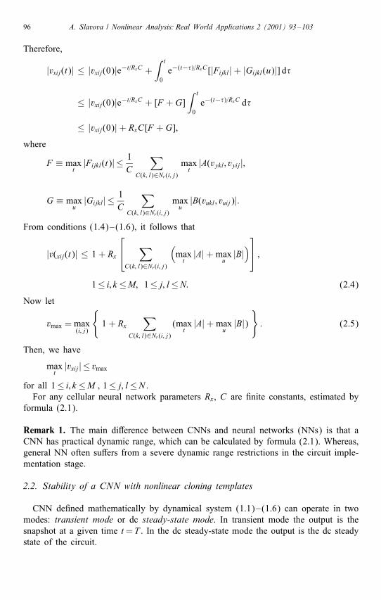
Therefore,

|vxij(t)| ≤ |vxij(0)|e−t=RxC +∫ t

0e−(t−�)=RxC[|Fijkl|+ |Gijkl(u)|] d�

≤ |vxij(0)|e−t=RxC + [F + G]∫ t

0e−(t−�)=RxC d�

≤ |vxij(0)|+ RxC[F + G];

where

F ≡ maxt

|Fijkl(t)| ≤ 1C


maxt

|A(vykl; vyij|;

G ≡ maxu

|Gijkl| ≤ 1C


maxu

|B(vukl; vuij)|:

From conditions (1.4)–(1.6), it follows that

|v(xij(t)| ≤ 1 + Rx

∑

C(k; l)∈Nr(i; j)

(max

t|A|+max

u|B|) ;

1≤ i; k ≤M; 1≤ j; l≤N: (2.4)

Now let

vmax = max(i; j)

{1 + Rx


(maxt

|A|+maxu

|B|)}

: (2.5)

Then, we have

maxt

|vxij| ≤ vmax

for all 1≤ i; k ≤M ; 1≤ j; l≤N .For any cellular neural network parameters Rx, C are �nite constants, estimated by

formula (2.1).

Remark 1. The main di�erence between CNNs and neural networks (NNs) is that aCNN has practical dynamic range, which can be calculated by formula (2.1). Whereas,general NN often su�ers from a severe dynamic range restrictions in the circuit imple-mentation stage.

2.2. Stability of a CNN with nonlinear cloning templates

CNN de�ned mathematically by dynamical system (1.1)–(1.6) can operate in twomodes: transient mode or dc steady-state mode. In transient mode the output is thesnapshot at a given time t=T . In the dc steady-state mode the output is the dc steadystate of the circuit.


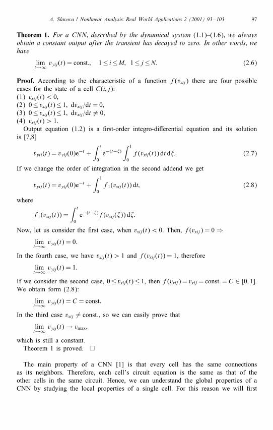
Theorem 1. For a CNN; described by the dynamical system (1:1)–(1:6); we alwaysobtain a constant output after the transient has decayed to zero. In other words; wehave

limt→∞ vyij(t) = const:; 1≤ i≤M; 1≤ j≤N: (2.6)

Proof. According to the characteristic of a function f(vxij) there are four possiblecases for the state of a cell C(i; j):(1) vxij(t)¡ 0,(2) 0≤ vxij(t)≤ 1; dvxij=dt = 0,(3) 0≤ vxij(t)≤ 1; dvxij=dt 6= 0,(4) vxij(t)¿ 1.Output equation (1.2) is a �rst-order integro-di�erential equation and its solution

is [7,8]

vyij(t) = vyij(0)e−t +∫ t

0e−(t−�)

∫ 1

0f(vxij(t)) dt d�: (2.7)

If we change the order of integration in the second addend we get

vyij(t) = vyij(0)e−t +∫ 1

0f1(vxij(t)) dt; (2.8)

where

f1(vxij(t)) =∫ t

0e−(t−�)f(vxij(�)) d�:

Now, let us consider the �rst case, when vxij(t)¡ 0. Then, f(vxij) = 0⇒limt→∞ vyij(t) = 0:

In the fourth case, we have vxij(t)¿ 1 and f(vxij(t)) = 1, therefore

limt→∞ vyij(t) = 1:

If we consider the second case, 0≤ vxij(t)≤ 1, then f(vxij) = vxij = const:=C ∈ [0; 1].We obtain form (2.8):

limt→∞ vyij(t) = C = const:

In the third case vxij 6= const., so we can easily prove thatlimt→∞ vyij(t)→ vmax;

which is still a constant.Theorem 1 is proved.

The main property of a CNN [1] is that every cell has the same connectionsas its neighbors. Therefore, each cell’s circuit equation is the same as that of theother cells in the same circuit. Hence, we can understand the global properties of aCNN by studying the local properties of a single cell. For this reason we will �rst


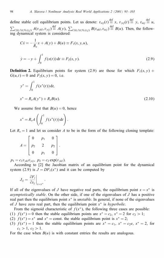
de�ne stable cell equilibrium points. Let us denote: vxij(t)def≡ x, vyij(t)

def≡ y, vuijdef≡ u,∑

C(k; l)∈Nr(i;j) A(vykl; vyij)def≡ A(y),

∑C(k; l)∈Nr(i;j) B(vukl; vuij)

def≡ B(u). Then, the follow-ing dynamical system is considered:

Cx =− 1Rx

x + A(y) + B(u) ≡ F1(x; y; u);

y =−y +∫ 1

0f(x(t)) dt ≡ F2(x; y): (2.9)

De�nition 2. Equilibrium points for system (2.9) are those for which F1(x; y) +G(u; t) = 0 and F2(x; y) = 0, i.e.

y∗ =∫ 1

0f(x∗(t)) dt;

x∗ = RxA(y∗) + RxB(u): (2.10)

We assume �rst that B(u) = 0, hence

x∗ = RxA

(∫ 1

0f(x∗(t)) dt

):

Let Rx = 1 and let us consider A to be in the form of the following cloning template:

A=

0 p1 0

p2 2 p2

0 p1 0

:

p1 = c1vyklvyij, p2 = c2 exp(vykl).According to [2] the Jacobian matrix of an equilibrium point for the dynamical

system (2.9) is J = DF1(x∗) and it can be computed by

Jij =@Fi

@xj

∣∣∣∣x=x∗

:

If all of the eigenvalues of J have negative real parts, the equilibrium point x = x∗ isasymptotically stable. On the other side, if one of the eigenvalues of J has a positivereal part then the equilibrium point x∗ is unstable. In general, if none of the eigenvaluesof J have zero real part, then the equilibrium point x∗ is hyperbolic.From the sigmoid characteristic of f(x∗), the following three cases are possible:

(1) f(x∗) = 0 then the stable equilibrium points are x∗ = c2, x∗ = 2 for c2¿ 1;(2) f(x∗) = x∗ and x∗ = const: the stable equilibrium point is x∗ = 2;(3) f(x∗) = 1 then the stable equilibrium points are x∗ = c1, x∗ = c2e, x∗ = 2, for

c1¿ 1, c2¿ 1.For the case when B(u) is with constant entries the results are analogous.


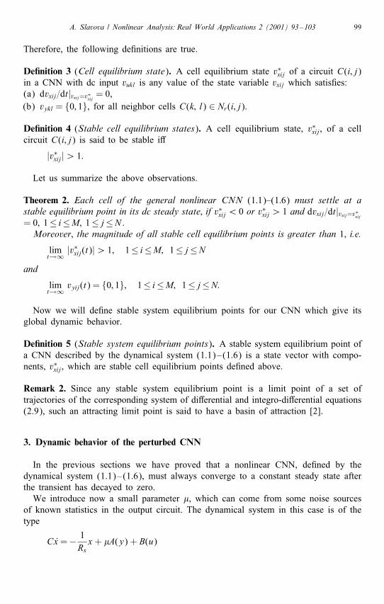
Therefore, the following de�nitions are true.

De�nition 3 (Cell equilibrium state). A cell equilibrium state v∗xij of a circuit C(i; j)in a CNN with dc input vukl is any value of the state variable vxij which satis�es:(a) dvxij=dt|vxij=v∗xij = 0,(b) vykl = {0; 1}, for all neighbor cells C(k; l) ∈ Nr(i; j).

De�nition 4 (Stable cell equilibrium states). A cell equilibrium state, v∗xij, of a cellcircuit C(i; j) is said to be stable i�

|v∗xij|¿ 1:

Let us summarize the above observations.

Theorem 2. Each cell of the general nonlinear CNN (1:1)–(1:6) must settle at astable equilibrium point in its dc steady state; if v∗xij ¡ 0 or v∗xij ¿ 1 and dvxij=dt|vxij=v∗xij= 0; 1≤ i≤M; 1≤ j≤N .Moreover; the magnitude of all stable cell equilibrium points is greater than 1; i.e.

limt→∞ |v∗xij(t)|¿ 1; 1≤ i≤M; 1≤ j≤N

and

limt→∞ vyij(t) = {0; 1}; 1≤ i≤M; 1≤ j≤N:

Now we will de�ne stable system equilibrium points for our CNN which give itsglobal dynamic behavior.

De�nition 5 (Stable system equilibrium points). A stable system equilibrium point ofa CNN described by the dynamical system (1.1)–(1.6) is a state vector with compo-nents, v∗xij, which are stable cell equilibrium points de�ned above.

Remark 2. Since any stable system equilibrium point is a limit point of a set oftrajectories of the corresponding system of di�erential and integro-di�erential equations(2.9), such an attracting limit point is said to have a basin of attraction [2].

3. Dynamic behavior of the perturbed CNN

In the previous sections we have proved that a nonlinear CNN, de�ned by thedynamical system (1.1)–(1.6), must always converge to a constant steady state afterthe transient has decayed to zero.We introduce now a small parameter �, which can come from some noise sources

of known statistics in the output circuit. The dynamical system in this case is of thetype

Cx=− 1Rx

x + �A(y) + B(u)


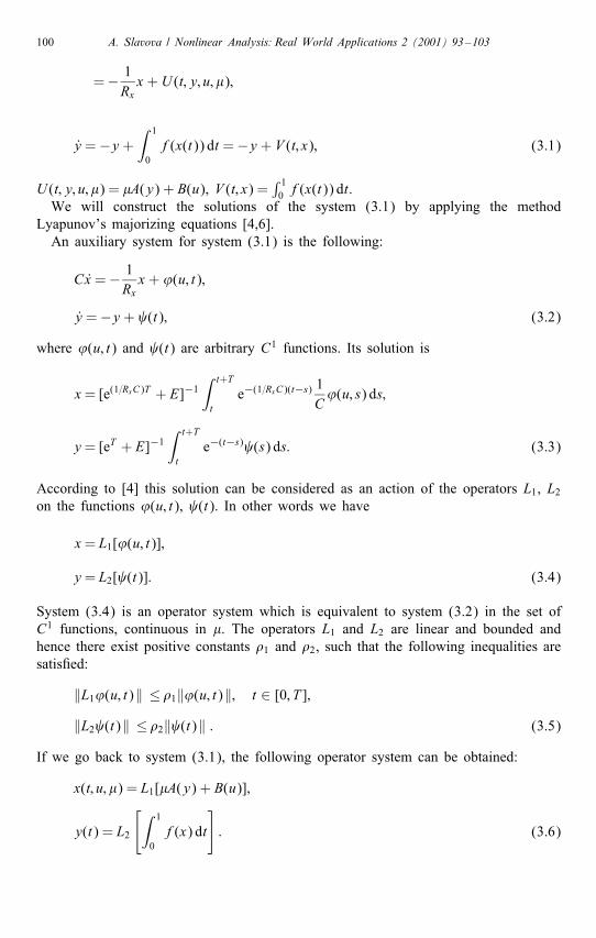
=− 1Rx

x + U (t; y; u; �);

y =−y +∫ 1

0f(x(t)) dt =−y + V (t; x); (3.1)

U (t; y; u; �) = �A(y) + B(u), V (t; x) =∫ 10 f(x(t)) dt.

We will construct the solutions of the system (3.1) by applying the methodLyapunov’s majorizing equations [4,6].An auxiliary system for system (3.1) is the following:

Cx =− 1Rx

x + ’(u; t);

y =−y + (t); (3.2)

where ’(u; t) and (t) are arbitrary C1 functions. Its solution is

x= [e(1=RxC)T + E]−1∫ t+T

te−(1=RxC)(t−s) 1

C’(u; s) ds;

y= [eT + E]−1∫ t+T

te−(t−s) (s) ds: (3.3)

According to [4] this solution can be considered as an action of the operators L1, L2on the functions ’(u; t), (t). In other words we have

x= L1[’(u; t)];

y= L2[ (t)]: (3.4)

System (3.4) is an operator system which is equivalent to system (3.2) in the set ofC1 functions, continuous in �. The operators L1 and L2 are linear and bounded andhence there exist positive constants �1 and �2, such that the following inequalities aresatis�ed:

‖L1’(u; t)‖ ≤ �1‖’(u; t)‖; t ∈ [0; T ];‖L2 (t)‖ ≤ �2‖ (t)‖ : (3.5)

If we go back to system (3.1), the following operator system can be obtained:

x(t; u; �) = L1[�A(y) + B(u)];

y(t) = L2

[∫ 1

0f(x) dt

]: (3.6)


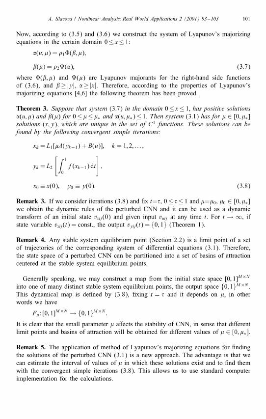
Now, according to (3.5) and (3.6) we construct the system of Lyapunov’s majorizingequations in the certain domain 0≤ x≤ 1:

�(u; �) = �1�(�; �);

�(�) = �2(�); (3.7)

where �(�; �) and (�) are Lyapunov majorants for the right-hand side functionsof (3.6), and �≥ |y|; �≥ |x|. Therefore, according to the properties of Lyapunov’smajorizing equations [4,6] the following theorem has been proved.

Theorem 3. Suppose that system (3:7) in the domain 0≤ x≤ 1; has positive solutions�(u; �) and �(�) for 0≤ �≤ �∗ and �(u; �∗)≤ 1. Then system (3:1) has for � ∈ [0; �∗]solutions (x; y); which are unique in the set of C1 functions. These solutions can befound by the following convergent simple iterations:

xk = L1[�A(yk−1) + B(u)]; k = 1; 2; : : : ;

yk = L2

[∫ 1

0f(xk−1) dt

];

x0 ≡ x(0); y0 ≡ y(0): (3.8)

Remark 3. If we consider iterations (3.8) and �x t=�, 0≤ �≤ 1 and �=�0, �0 ∈ [0; �∗]we obtain the dynamic rules of the perturbed CNN and it can be used as a dynamictransform of an initial state vxij(0) and given input vuij at any time t. For t → ∞, ifstate variable vxij(t) = const:, the output vyij(t) = {0; 1} (Theorem 1).

Remark 4. Any stable system equilibrium point (Section 2.2) is a limit point of a setof trajectories of the corresponding system of di�erential equations (3.1). Therefore,the state space of a perturbed CNN can be partitioned into a set of basins of attractioncentered at the stable system equilibrium points.

Generally speaking, we may construct a map from the initial state space [0; 1]M×N

into one of many distinct stable system equilibrium points, the output space {0; 1}M×N .This dynamical map is de�ned by (3.8), �xing t = � and it depends on �, in otherwords we have

F�: [0; 1]M×N → {0; 1}M×N :

It is clear that the small parameter � a�ects the stability of CNN, in sense that di�erentlimit points and basins of attraction will be obtained for di�erent values of � ∈ [0; �∗].

Remark 5. The application of method of Lyapunov’s majorizing equations for �ndingthe solutions of the perturbed CNN (3.1) is a new approach. The advantage is that wecan estimate the interval of values of � in which these solutions exist and to �nd themwith the convergent simple iterations (3.8). This allows us to use standard computerimplementation for the calculations.


Fig. 1.

In general, it is di�cult if not impossible to predict the behavior of complex nonlineardynamical systems, but our analysis shows that we can prove the existence and �nd thesolutions of the perturbed CNN by using method of Lyapunov’s majorizing equations.

4. Example and computer implementation

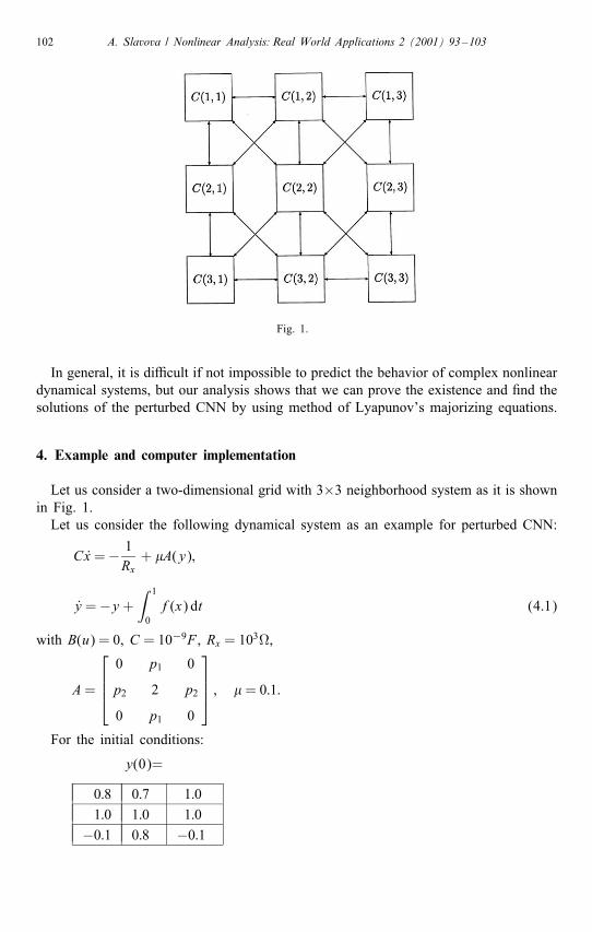
Let us consider a two-dimensional grid with 3×3 neighborhood system as it is shownin Fig. 1.Let us consider the following dynamical system as an example for perturbed CNN:

Cx =− 1Rx+ �A(y);

y =−y +∫ 1

0f(x) dt (4.1)

with B(u) = 0, C = 10−9F , Rx = 103,

A=

0 p1 0

p2 2 p2

0 p1 0

; � = 0:1:

For the initial conditions:

y(0)=

0:8 0:7 1:01:0 1:0 1:0

−0:1 0:8 −0:1


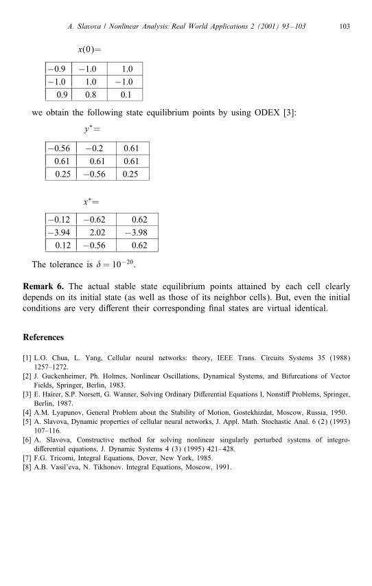
x(0)=

−0:9 −1:0 1:0−1:0 1:0 −1:00:9 0:8 0:1

we obtain the following state equilibrium points by using ODEX [3]:

y∗=

−0:56 −0:2 0:610:61 0:61 0:610:25 −0:56 0:25

x∗=

−0:12 −0:62 0:62−3:94 2:02 −3:980:12 −0:56 0:62

The tolerance is �= 10−20.

Remark 6. The actual stable state equilibrium points attained by each cell clearlydepends on its initial state (as well as those of its neighbor cells). But, even the initialconditions are very di�erent their corresponding �nal states are virtual identical.

References

[1] L.O. Chua, L. Yang, Cellular neural networks: theory, IEEE Trans. Circuits Systems 35 (1988)1257–1272.

[2] J. Guckenheimer, Ph. Holmes, Nonlinear Oscillations, Dynamical Systems, and Bifurcations of VectorFields, Springer, Berlin, 1983.

[3] E. Hairer, S.P. Norsett, G. Wanner, Solving Ordinary Di�erential Equations I, Nonsti� Problems, Springer,Berlin, 1987.

[4] A.M. Lyapunov, General Problem about the Stability of Motion, Gostekhizdat, Moscow, Russia, 1950.[5] A. Slavova, Dynamic properties of cellular neural networks, J. Appl. Math. Stochastic Anal. 6 (2) (1993)

107–116.[6] A. Slavova, Constructive method for solving nonlinear singularly perturbed systems of integro-

di�erential equations, J. Dynamic Systems 4 (3) (1995) 421–428.[7] F.G. Tricomi, Integral Equations, Dover, New York, 1985.[8] A.B. Vasil’eva, N. Tikhonov. Integral Equations, Moscow, 1991.

stability analysis of cellular neural networks with nonlinear dynamics

Documents