sst dependence of the pma emission - atmos-chem-phys ... fileacpd 14, 377–434, 2014 sst dependence...

ACPD14, 377–434, 2014

SST dependence ofthe PMA emission

S. Barthel et al.

Title Page

Abstract Introduction

Conclusions References

Tables Figures

J I

J I

Back Close

Full Screen / Esc

Printer-friendly Version

Interactive Discussion

Discussion

Paper

|D

iscussionP

aper|

Discussion

Paper

|D

iscussionP

aper|

Atmos. Chem. Phys. Discuss., 14, 377–434, 2014www.atmos-chem-phys-discuss.net/14/377/2014/doi:10.5194/acpd-14-377-2014© Author(s) 2014. CC Attribution 3.0 License.

Atmospheric Chemistry

and Physics

Open A

ccess

Discussions

This discussion paper is/has been under review for the journal Atmospheric Chemistryand Physics (ACP). Please refer to the corresponding final paper in ACP if available.

Model study on the dependence ofprimary marine aerosol emission on thesea surface temperatureS. Barthel, I. Tegen, R. Wolke, and M. van Pinxteren

Leibniz Institute for Tropospheric Research, Permoser Straße 15, 04318 Leipzig, Germany

Received: 13 November 2013 – Accepted: 16 December 2013 – Published: 7 January 2014

Correspondence to: S. Barthel ([email protected]) and I. Tegen ([email protected])

Published by Copernicus Publications on behalf of the European Geosciences Union.

377

http://www.atmos-chem-phys-discuss.net

http://www.atmos-chem-phys-discuss.net/14/377/2014/acpd-14-377-2014-print.pdf

http://www.atmos-chem-phys-discuss.net/14/377/2014/acpd-14-377-2014-discussion.html

http://creativecommons.org/licenses/by/3.0/

ACPD14, 377–434, 2014


S. Barthel et al.

Title Page



Tables Figures

J I

J I

Back Close

Full Screen / Esc



Discussion

Paper

|D

iscussionP

aper|

Discussion

Paper

|D

iscussionP

aper|

Abstract

Primary marine aerosol composed of sea salt and organic material is an importantcontributor to the global aerosol load. By comparing measurements from two EMEP(co-operative programme for monitoring and evaluation of the long-range transmissionsof air-pollutants in Europe) intensive campaigns in June 2006 and January 2007 with5

results from an atmospheric transport model this work shows that accounting for theinfluence of the sea surface temperature on the emission of primary marine aerosolimproves the model results towards the measurements in both months. Different seasurface temperature dependencies were evaluated. Using correction functions basedon Sofiev et al. (2011) and Jaeglé et al. (2011) improves the model results for coarse10

mode particles. In contrast, for the fine mode aerosols no best correction function couldbe found. The model captures the low sodium concentrations at the marine stationVirolahti II (Finland), which is influenced by air masses from the low salinity Baltic Sea,as well as the higher concentrations at Cabauw (Netherlands) and Auchencorth Moss(Scotland). These results indicate a shift towards smaller sizes with lower salinity for the15

emission of dry sea salt aerosols. Organic material was simulated as part of primarymarine aerosol assuming an internal mixture with sea salt. A comparison of the modelresults for primary organic carbon with measurements by a Berner-impactor at SaoVincente (Cape Verde) indicated that the model underpredicted the observed organiccarbon concentration. This leads to the conclusion that the formation of secondary20

organic material needs to be included in the model to improve the agreement with themeasurements.

1 Introduction

Sea salt dominates the aerosol mass in the marine atmosphere (O’Dowd and deLeeuw, 2007). Due to their high hygroscopicity sea salt aerosol (SSA) particles can25

be easily activated and act as cloud condensation nuclei (CCN) (Pruppacher and Klett,

378





ACPD14, 377–434, 2014


S. Barthel et al.

Title Page



Tables Figures

J I

J I

Back Close

Full Screen / Esc



Discussion

Paper

|D

iscussionP

aper|

Discussion

Paper

|D

iscussionP

aper|

1997; O’Dowd and Smith, 1993; Quinn et al., 1998; Murphy et al., 1998; Pierce andAdams, 2006). Sea salt droplets take part in heterogeneous chemical and microphys-ical transformations, thus influencing traces gases in the marine boundary layer (e.g.,von Glasow et al., 2002). SSA also impacts the incoming radiation. In clear sky condi-tions it dominates the aerosol extinction of solar radiation over larger parts of the ocean,5

regionally contributing more than 75% to the aerosol scattering (Haywood et al., 1999;Grini et al., 2002; Ma et al., 2008; Murphy et al., 1998). Its direct radiative effect is stillhighly uncertain (Lundgren et al., 2013), which is also reflected in the uncertainty inestimates of reduction of the radiation absorbed by the ocean between 0.08–6 Wm−2

(Lewis and Schwartz, 2004).10

In addition to sea salt (SS), primary marine aerosol (PMA) can contain organic mate-rial (OM) (e.g, O’Dowd et al., 2004). The OM changes cloud condensation nuclei prop-erties (Roelofs, 2008; Fuentes et al., 2010; Meskhidze et al., 2011; Westervelt et al.,2012), the direct and indirect radiative effects (Gantt et al., 2012a) and the aerosolchemistry (Smoydzin and von Glasow, 2007) compared to SS only.15

Estimates of PMA distribution and effects are highly uncertain. A global sourcestrength of 5000Tgyr−1 with a uncertainty factor of 4 has been reported by Lewisand Schwartz (2004). A comparison of different models showed global emission ratesbetween 3 and 18Tgyr−1 (Textor et al., 2006). The high diversities in the modelled SSemission rates may be caused by insufficient process parameterisation of the emis-20

sion in the currently available SS source functions. The main driver of PMA emissionis the surface wind speed. While Ma et al. (2008) and Fan and Toon (2011) found noimpact of the water temperature on the PMA emission fluxes, the parameterisationsof Mårtensson et al. (2003), Jaeglé et al. (2011) and Sofiev et al. (2011) include thedependence on the sea surface temperature (SST). Jaeglé et al. (2011) and Sofiev25

et al. (2011) showed the importance of the temperature dependence for SS emissionflux calculations at the global scale. At the regional scale this is indicated by the resultsof Tsyro et al. (2011). However, different measurements disagree in the resulting SSTinfluence on PMA emission.

379





ACPD14, 377–434, 2014


S. Barthel et al.

Title Page



Tables Figures

J I

J I

Back Close

Full Screen / Esc



Discussion

Paper

|D

iscussionP

aper|

Discussion

Paper

|D

iscussionP

aper|

This study investigates the effect of SST-correction of the PMA emission flux for re-gional modelling. The correction functions for the PMA emission flux accounting forthe SST by Jaeglé et al. (2011), Sofiev et al. (2011) and in addition a new param-eterisation derived from Zábori et al. (2012) are compared with each other and withmeasurements from two intensive campaigns within the EMEP network in June 20065

and January 2007 as well as Berner-impactor measurements made at the Cape VerdeAtmospheric Observatory at Sao Vincente in December 2007. The model simulationswere carried out with the regional chemistry and aerosol transport model COSMO-MUSCAT (COnsortium of Small scale MOdelling – MUlti-Scale Chemical and AerosolTransport model) for an “European” region including Iceland and an “African” region.10

2 PMA emission processes

Two processes are mainly responsible for PMA emission. These are the tearing ofdrops from wave crests and the bursting of bubbles, which are formed by the entrain-ment of air to the ocean through breaking waves. The dislocation of water dropletsfrom the wave crest occurs only at 10 m wind speeds above 7–11 ms−1, producing the15

largest sea spray particles (“spume droplets” Monahan et al., 1983) with a minimumdiameter of 40µm and no defined maximum (Andreas, 1998). Such large droplets havehigh deposition and sedimentation velocities resulting in low residence times. There-fore they are less important for atmospheric microphysical and chemical processes andare usually neglected in large scale modelling.20

The bubble bursting process is caused by bubbles rising back to the surface afterthe entrainment of air to the ocean. They emit two sorts of primary aerosols: small filmdroplets and larger jet droplets (Blanchard, 1963). Film droplets are formed during thecollapse of a bubble from the water film, or cap of its top. During that process, up toa few hundred film droplets are produced per bubble. At 80% relative humidity these25

droplets have typical radii of r80 = 1µm and less (Lewis and Schwartz, 2004). Spiel(1998) found that film droplets are emitted mainly by bigger bubbles with a bubble ra-

380





ACPD14, 377–434, 2014


S. Barthel et al.

Title Page



Tables Figures

J I

J I

Back Close

Full Screen / Esc



Discussion

Paper

|D

iscussionP

aper|

Discussion

Paper

|D

iscussionP

aper|

dius R > 2mm. The second type, the jet droplets are emitted from a vertical jet emerg-ing from the bottom of the bubble. Up to 6–10 jet droplets per bubble (Mårtensson et al.,2003; Blanchard, 1983) are emitted by bubbles with radius R < 3.4mm (Mårtenssonet al., 2003). Their size distribution has its maximum around r80 = 4µm (O’Dowd andSmith, 1993).5

The emission of PMA by bursting bubbles is influenced by parameters that controlthe bubble number and size distribution as well as parameters influencing the wavebreaking activity. This includes the entrainment depth, SST, salinity or generally thecomposition of the water regarding OM or rather surfactants in the surface water. Wavebreaking activity is controlled by the surface wind speed, wind fetch, wave height or the10

ocean bottom conditions (Lewis and Schwartz, 2004, and citations therein).

2.1 Wind speed dependence

Surface wind speed (10m) is the only parameter controlling the emission rate in most ofthe SSA emission functions (Monahan et al., 1986; Smith et al., 1993; Smith and Har-rison, 1998; Gong, 2003; Clarke et al., 2006). Wind stress at the ocean surface causes15

wave formation and wave breaking, leading to the entrainment of air and the produc-tion of bubbles in the ocean, but also causes the tearing of droplets from wave crests.Its impact on wave height and thus surface roughness length influences the verticaltransport of aerosols by turbulence and thereby controlling the effective PMA produc-tion. The PMA production through bubble bursting has been found to be dependent20

on the particle production per whitecap area and the whitecap coverage, which wereassumed to be independent from each other by Monahan et al. (1986) and Mårtens-son et al. (2003), who treated only the whitecap coverage to be dependent on the windspeed. Mårtensson et al. (2003) found that the function F ∝ U3.41

10 of Monahan andO’Muircheartaigh (1980) for the whitecap coverage resulted in the most similar slope25

to the measurements by Nilsson et al. (2001), compared to others. Here, F stands forthe particle flux and U10 for the wind speed at a height of 10 m. Keene et al. (2007)found the production of marine aerosol through bubble bursting to be proportional to

381





ACPD14, 377–434, 2014


S. Barthel et al.

Title Page



Tables Figures

J I

J I

Back Close

Full Screen / Esc



Discussion

Paper

|D

iscussionP

aper|

Discussion

Paper

|D

iscussionP

aper|

the amount of air detrained from the water column. With the assumption that all air,which entrains into the water column detrains as bubbles, the dependency F ∝ U3.74

10was found (Long et al., 2011). This exponent is nearly the same as found by Wu (1979)for the whitecap dependency on surface wind speed.

2.2 Enrichment with organic material5

OM can be an important part of PMA (e.g., Blanchard, 1964). Current parameterisa-tions (Gantt et al., 2012b, and citations therein) afford a quantification of the amountof organics in the aerosols. Although many components and chemical species couldbe found, a large fraction is still unknown (e.g. Gantt and Meskhidze, 2013). Thisleads to considerable model uncertainties by using OM as universal tracer (Roelofs,10

2008; Fuentes et al., 2010; Meskhidze et al., 2011; Westervelt et al., 2012; Gantt et al.,2012a). The fraction of OM in the PMA is found to be proportional to the primary pro-duction near the oceanic surface traced by the chlorophyll a concentration (O’Dowdet al., 2004; Sciare et al., 2009) and inversely proportional to the aerosol diameter(Barker and Zeitlin, 1972; Hoffmann and Duce, 1977; Oppo et al., 1999; O’Dowd et al.,15

2004; Rinaldi et al., 2009). The surface wind speed can further influence the organic toSS mass ratios in PMA (Gantt et al., 2011, and citations therein). The organic fractionin the oceanic surface water increases towards the surface (e.g. Russel et al., 2010)and forms surface films (Hardy, 1982) including surface-active material (Duce and Hoff-mann, 1976). These surface films exist only under calm wind conditions and break up20

at 10 m wind speeds above 8ms−1 (Carlson, 1983). They can lead to wave suppres-sion (Sellegri et al., 2006) resulting in lower emission rates. At higher wind speedsthe concentration of organics in PMA is lower due to decreased near-surface concen-tration through stronger oceanic mixing. The surface active material surrounds the airbubbles in the water thus decreasing the gas exchange rate between the bubble and25

the water and increasing the rising speed of the bubbles (Lewis and Schwartz, 2004),resulting in changes in the bubble size spectra. Furthermore it stabilises the bubbles at

382





ACPD14, 377–434, 2014


S. Barthel et al.

Title Page



Tables Figures

J I

J I

Back Close

Full Screen / Esc



Discussion

Paper

|D

iscussionP

aper|

Discussion

Paper

|D

iscussionP

aper|

the ocean surface and allows them to thin out before bursting, which results in a shiftof the particle spectra towards smaller sizes (Sellegri et al., 2006; Modini et al., 2013).

Summarising different measurements, Gantt and Meskhidze (2013) concluded thatOM can displace SS or act as additional material in the emitted aerosols. This contri-bution is size dependend (Gantt and Meskhidze, 2013). Due to the lack of knowledge5

of a detailed quantification of that effect, it was decided to treat PMA as internal mixturewith SS being replaced by OM for this work. With this assumption the volume of thetotal emitted PMA VP is is represented by:

VP = VSS + VOM , (1)

where VSS and VOM stands for the volumes of dry SS and OM respectively. The volume10

ratio RV between OM and SS is expressed as:

RV =VOM

VSS(2)

and the ratio RVp between OM and dry PMA:

RVp =VOM

VP. (3)

2.3 Dependence of PMA emission on SST15

The SST can influence the physical processes controlling the PMA emission fluxthrough bubble bursting via the viscosity of the water, the surface tension at the bound-ary between water and air, the molecular diffusivity and the solubility of gases. Theseproperties impact on the coalescence of the bubbles, the gas exchange between thebubble and the surrounding water and the rising speed and thus the residence time of20

a bubble.The kinematic viscosity of water decreases by a factor 2.2 with a temperature change

from 0 to 30 ◦C (e.g., Chen et al., 1973). This leads to a 2.2 times lower rise speed of383





ACPD14, 377–434, 2014


S. Barthel et al.

Title Page



Tables Figures

J I

J I

Back Close

Full Screen / Esc



Discussion

Paper

|D

iscussionP

aper|

Discussion

Paper

|D

iscussionP

aper|

air bubbles at 0 ◦C due to the inverse proportional relationship assuming Stokes motion(Lewis and Schwartz, 2004). The resulting higher residence time in cold waters leadsto an increase in the coalescence of bubbles, thus decreasing the number of smallerbubbles and increasing the number of bigger bubbles (Pounder, 1986).

The higher solubility of gases at cold temperatures in combination with the higher5

residence time of the bubbles lead to higher gas exchange rates between the bubbleand the surrounding water. This is partly compensated by the lower diffusivity (Thropeet al., 1992). The gas exchange leads to a shrinking of the bubbles during their riseto the ocean surface. Smaller bubbles dissolve completely while bigger bubbles cansurvive. Higher exchange rates in colder waters lead to a decrease in the number of10

smaller bubbles resulting in a shift of the bubble size distribution towards bigger bubbles(see also Sect. 4.4.2., Fig. 35 Lewis and Schwartz, 2004).

Surface tension decreases only by 6% for temperature changes between 0 and30 ◦C, but may also impact the PMA emission. It may influence the breakup of bubblesin the water, bubble shape and the rising velocity as well as the breakup processes at15

the surface (Blanchard, 1963; Lewis and Schwartz, 2004).In summary, lower SST lead to a decrease in the number concentration of small and

an increase of large bubbles, resulting in a shift in the PMA size distribution.Several laboratory studies confirm the influence of the SST on PMA emission

(Bowyer et al., 1990; Mårtensson et al., 2003; Sellegri et al., 2006; Hultin et al., 2011;20

Zábori et al., 2012). Disagreements in the studies may be due to differences in theexperimental setup. All authors found an increase in the number concentrations ofsmall particles with decreasing temperature. Zábori et al. (2012) found a up to 10-foldincrease for particles with diameter between 0.012µm and 1.8µm when reducing tem-peratures from 13–16 ◦C to 0 ◦C. Similarly Hultin et al. (2011) and Bowyer et al. (1990)25

also found a 4 to 5 times increasing particle number concentration with decreasing tem-perature for particles with a dry diameter of 0.02µm to 1.8µm and 0.25µm to 1.5µmrespectively. Finally, Mårtensson et al. (2003) also found an increase up to a size of0.1µm in dry diameter with a continuous increase of the factor with decreasing particle

384





ACPD14, 377–434, 2014


S. Barthel et al.

Title Page



Tables Figures

J I

J I

Back Close

Full Screen / Esc



Discussion

Paper

|D

iscussionP

aper|

Discussion

Paper

|D

iscussionP

aper|

size. In contrast Zábori et al. (2012) found a local maximum factor between 0.18µmand 0.57µm at the maximum of the measured size distributions.

For particles bigger than 1.8µm Zábori et al. (2012) observed constant number con-centrations. In contrast, Bowyer et al. (1990) found a decrease by factor 2–3 for parti-cles bigger than 1.5µm with decreasing temperature. Sofiev et al. (2011) extrapolated5

the data of Mårtensson et al. (2003), which only included particles smaller than 2.8µm,to larger particles and derived a factor of 4.5 for 2µm and 10.5 for 10µm between 5and 15 ◦C.

While Mårtensson et al. (2003) found the number concentration of all particle sizeschanged for all measured water temperatures, Zábori et al. (2012) found it to be con-10

stant above 10 ◦C. Hultin et al. (2011) and Bowyer et al. (1990) also found a constantnumber concentration above 14–15 ◦C for particles with dry diameter 0.02–2.8µm and0.25 to 2.5µm, respectively.

2.3.1 Parameterisation of the SST correction factor

Two parameterisations of the temperature dependence of the PMA emission are cur-15

rently available by Jaeglé et al. (2011) and Sofiev et al. (2011). Jaeglé et al. (2011)(thereafter named J11) compared measurements, which were made during six cruisesconducted by NOAA’s Pacific Marine Environmental Laboratory with model results.They found a strong relationship between the ratio of measured to modelled SSA-concentration and the SST. The model underestimated the measured ratios over water20

with a SST TW > 25 ◦C and overestimated them over water with a SST TW < 10 ◦C. Witha third-order polynomial fit of the ratio between observation and model results they de-veloped a correction function cJ for the temperature dependence of the SSA emissionfluxes F (TW) = c(TW)F0, where F0 is the uncorrected emission flux:

cJ (TW) = 0.3+0.1 · TW −0.0076 · TW +0.00021 · TW , (4)25

with TW in ◦C. cJ is independent of particle size and shifts from reducing to raising theemission rates at a water temperature around 21 ◦C. The second parameterisation by

385





ACPD14, 377–434, 2014


S. Barthel et al.

Title Page



Tables Figures

J I

J I

Back Close

Full Screen / Esc



Discussion

Paper

|D

iscussionP

aper|

Discussion

Paper

|D

iscussionP

aper|

Sofiev et al. (2011) (S11) was derived from the laboratory measurements of Mårtens-son et al. (2003). Assuming the SSA flux needs no correction at the temperature of25 ◦C the measured fluxes at TW = 15 ◦C,5 ◦C and −2 ◦C were divided by F (25 ◦C). Theresulting data were fitted by power law functions:

cS(TW,Dp) = a(TW) ·Db(TW)p , (5)5

where Dp stands for the dry particle diameter and the parameters a and b are given inTable 1.

For SST other than in Table 1 the values for cS are derived by linear interpolation.This parameterisation is derived for the size range of 0.02 to 6–7 µm but applied to thesize range of 0.01 to 10µm in the model, which leads to uncertainties in the emission10

fluxes (Sofiev et al., 2011).Since the shape of the size distribution for smaller particles differs strongly from

the results by Zábori et al. (2012) a further parameterisation based on that data wastested, using the setup with 35‰ salinity and no surfactants. In those experiments thewater temperature was slowly increased resulting in differing PMA size distributions.15

These size distributions were fitted with five lognormal distributions, which are used togenerate the SST-correction function. Only the 0 ◦C- and the 13–16 ◦C-distributions areused by dividing them through each other similar to the method of Sofiev et al. (2011).It is assumed that the original PMA emission flux parameterisations are valid at thehigher temperature. This result can be fitted by a further lognormal distribution for the20

factor cZb:

cZb(0 ◦C,Dp) =dc0

dDp=

4.492√

2 ·Π ·Dp ·0.471·exp

−0.5 ·(

log10Dp − log10 0.44

0.471

)2 (6)

or

cZb(0 ◦C,Dp) =dc0

dlogDp=

18.386√

2 ·Π ·0.471·exp

−0.5 ·(

log10Dp − log10 0.136

0.471

)2 , (7)

386





ACPD14, 377–434, 2014


S. Barthel et al.

Title Page



Tables Figures

J I

J I

Back Close

Full Screen / Esc



Discussion

Paper

|D

iscussionP

aper|

Discussion

Paper

|D

iscussionP

aper|

where c0 is the ratio between 0 ◦C and the 13–16 ◦C-distribution. Because of the lowrelative humidity in these experiments of 21–29 % and the deliquescence point of SSat 40%, Dp is taken to be the dry particle diameter in µm.

To take the temperature dependence into account, an interpolation between thevalue given by these equations at 0 ◦C and cZb(13 ◦C,Dp) = 1 was carried out. An expo-5

nential fit was selected, because the other two size distributions of Zábori et al. (2012)in the temperature ranges of 1–4 ◦C and 8–11 ◦C were reproduced at 2.6 ◦C and 12.2 ◦Cbetter than with a linear fit (5.7 ◦C and 12.8 ◦C). Other fits were not possible due to in-sufficient data. Since Zábori et al. (2012) found no further influence for temperaturesabove 10 ◦C (8–14 ◦C depending on experimental setup) cZb is set to 1 for all temper-10

atures above 13 ◦C. This function based on Zábori et al. (2012) is further denoted asZb13. The different correction functions are compared in Fig. 1.

3 Methods

3.1 Emission parameterisation

There is a wide variety of different parameterisations of SSA or PMA emissions (e.g.15

de Leeuw et al., 2011). The SS source function by Monahan et al. (1986) is known toprovide good results in the bubble-derived size range (e.g., Andreas, 1998) except forparticles smaller than 0.5µm in dry diameter (Schulz et al., 2004). Newer parameteri-sations are normally evaluated against that source function (Gong, 2003; Mårtenssonet al., 2003; Clarke et al., 2006; Long et al., 2011; Sofiev et al., 2011), or it is part of20

an emission function (e.g. Lundgren et al., 2013, which uses Mårtensson et al., 2003;Monahan et al., 1986; Smith et al., 1993). A comparison of the volume emission fluxof four different source functions in Fig. 2 shows comparable results in the mid-sizerange. However, they differ strongly for the small and the large particles. During labo-ratory experiments it could be shown that particles as small as 10nm can be produced25

by bubble bursting (Mårtensson et al., 2003; Sellegri et al., 2006). The four source

387





ACPD14, 377–434, 2014


S. Barthel et al.

Title Page



Tables Figures

J I

J I

Back Close

Full Screen / Esc



Discussion

Paper

|D

iscussionP

aper|

Discussion

Paper

|D

iscussionP

aper|

functions differ from each other in total number and shape of the size distribution forparticles smaller than 100nm. The highest emission rates are found for Long et al.(2011) and the smallest for Gong (2003) parameterization in that size range.

The Long et al. (2011)-parameterisation retrieved the best results in the compari-son to measurements with a Berner-impactor at Sao Vincente (Cape Verde), and was5

chosen as basic emission function in this work. This source function uses a 2 modeapproach for the description of the size distribution:

dfNum

dlog10Dp80= FEnt ·10PN (8)

where FEnt is the term for the wind speed dependence (below), fNum the particle numberflux in m−2 s−1, Dp80 the particle diameter at 80% relative humidity in µm and PN is10

represented by the two modes, separated at 1µm:

P1 =1.46 · (log10(Dp80))3 +1.33 · (log10(Dp80))2 −1.82 · (log10(Dp80))+8.83

for Dp80 < 1µm

P2 =−1.53 · (log10(Dp80))3 −8.1 · (log10(Dp80))2 −4.26 · (log10(Dp80))+8.84

for Dp80 > 1µm

(9)

Long et al. (2011) parameterized the wind speed influence on the particle productionwith the entrainment of air into the water column:15

FEnt = 2×10−8 ·U3.7410 (10)

For mixed PMA, Long et al. (2011) calculated the pure SS part of a particle sizeto determine emission rates. Since PMA is treated here as internal mixture withoutinfluence of the OM on the emission rates, we assume the total particle size to becomposed of both SS and OM.20

The dry SSA production depends on the salinity of the ocean water, which has to beconsidered while calculating the emission fluxes. The emission function of Long et al.

388





ACPD14, 377–434, 2014


S. Barthel et al.

Title Page



Tables Figures

J I

J I

Back Close

Full Screen / Esc



Discussion

Paper

|D

iscussionP

aper|

Discussion

Paper

|D

iscussionP

aper|

(2011) is based on the measurements of Keene et al. (2007) and Faccini et al. (2008).Keene et al. (2007) used sea water from the Bermuda Islands and Faccini et al. (2008)sampled aerosols 400km off the Irish west coast. So in summary the salinity is approx-imately 35‰. To use this emission function for other salinities a corresponding particlesize has to be calculated. It is assumed that the particle size is independent of salinity5

in the moment of the formation (RH = 98%). With that assumption the source functiondefines the emission flux and the salinity the corresponding dry particle size. This willlead to a shift of the emitted particle size distributions towards smaller diameters forlower salinities, as reported by Zábori et al. (2012). No further influence of the salinityon the number production or size distribution (Mårtensson et al., 2003; Sofiev et al.,10

2011) has been taken into account.The PMA emission schemes account for the fluxes at the measurement height, which

is a few centimetres in case of laboratory bubble bursting experiments (Monahan et al.,1986; Bowyer et al., 1990; Mårtensson et al., 2003; Sellegri et al., 2006; Long et al.,2011) or a few meters in oceanic field studies (Smith et al., 1993; Smith and Harrison,15

1998; Clarke et al., 2006). Therefore it is difficult to compare the source functions witheach other because large particles quickly settle after emission. Thus the effectivefluxes are calculated at a defined height. For this an equation by Hoppel et al. (2005)can be used:

F (z2)

F (z1)=(z2

z1

)−( vsκ ·u∗

)(11)20

where F is the PMA flux at the heights z1 and z2, vs the sedimentation velocity ofthe particle at 80 % relative humidity, κ the von Kaarman constant and u∗ the frictionvelocity. For the height correction of surface fluxes we set z1 = z0, where z0 is thesurface roughness length. z0 and u∗ are taken from the meteorological driver modelCOSMO (see below). Due to the gravitational losses only particles reaching the half25

level height of the lowest level (z1/2) are taken into account, thus z2 = z1/2 (Fan andToon, 2011).

389





ACPD14, 377–434, 2014


S. Barthel et al.

Title Page



Tables Figures

J I

J I

Back Close

Full Screen / Esc



Discussion

Paper

|D

iscussionP

aper|

Discussion

Paper

|D

iscussionP

aper|

To calculate the organic mass emitted with SS few parameterisations are available,which are summarised in a comparison study by Gantt et al. (2012b). Here the param-eterisation by Long et al. (2011) is used together with the assumption that OM replacesSS in the emitted aerosols. For the calculation of the volume ratio RV of OM to dry SS(compare Eq. 2) Long et al. (2011) used the two-mode approach that was mentioned5

above:For Dp80 < 1µm:

RV,1(Dp80,chl a) = 0.306 ·Dδ1

p80 (12)

with

δ1 =−2.01 ·40 · [chl a]

1+40 · [chl a](13)10

and for Dp80 > 1µm:

RV,2(Dp80,chl a) =0.056 ·20.8 · [chl a]

1+29.8 · [chl a]. (14)

The variables Dp80 and chl a represent the particle size at 80 % relative humidity in

µm and the chlorophyll a concentration at the ocean surface in µgL−1.

3.2 COSMO-MUSCAT15

For this study the multi scale model system COSMO-MUSCAT (Wolke et al., 2012) isused. It was developed for process studies and operational forecast of pollutants andhas been used in several air quality studies (Renner and Wolke, 2010) as well as largescale-transport studies of Saharan dust (Heinold et al., 2011). It is a online coupledsystem of COSMO developed by the German Weather Service (DWD) (Schättler et al.,20

2008) and MUSCAT (Wolke et al., 2012). The small-scale weather model COSMO is390





ACPD14, 377–434, 2014


S. Barthel et al.

Title Page



Tables Figures

J I

J I

Back Close

Full Screen / Esc



Discussion

Paper

|D

iscussionP

aper|

Discussion

Paper

|D

iscussionP

aper|

the operational weather forecast model at DWD. It is used as driver for the meteorolog-ical input fields. For the initialisation and the boundary data of COSMO, the model sim-ulations within this work used reanalysis data from GME (Global Model Earth) of theDWD, which were updated every three model hours. The chemistry-transport modelMUSCAT treats aerosol and gas phase transport processes and chemical transfor-5

mations. The transport processes in the model include advection, turbulent diffusion,sedimentation and size dependent dry and wet deposition as well as chemical andmicrophysical transformations (not regarded in this work) (Wolke et al., 2012). Theaerosol size distribution is described with a mass based approach. This approach wasextended for PMA to a spectral distribution using 15 logarithmically spaced bins which10

spread over the size range for the dry diameter from 0.01 to 10µm. This number of binshas been chosen to optimize accuracy at reasonable computing times.

PMA emission fluxes are calculated using the parameterisation of Long et al. (2011)(Eqs. 9 and 10) assuming an internal mixture of OM and SS. The ratio of OM and SS ateach size bin is also taken from Long et al. (2011) (Eqs. 12–14). The correction for the15

effective flux is described by Eq. (11). The salinity dependence of PMA emissions wasaccounted for through the calculation of the corresponding particle size at formation forboth, the emitted particle at the actual salinity and the source function, where salinityis assumed at 35‰.

The removal processes are described by dry and wet deposition. For the dry depo-20

sition, the resistance approach is used (Seinfeld and Pandis, 2006), that accounts foratmospheric turbulence, aerodynamic and quasi-laminar layer resistance and gravita-tional settling. Dry deposition velocities are size dependent and calculated for everybin. Therefore the size bins are represented by the geometric mean radius with theaddition of water according to Eq. (15) (below). Wet deposition is distinguished into25

washout, which describes the uptake of gases and particles by falling hydrometeorsbelow clouds, and rainout, which accounts for the absorption of gases and particles bydroplets within the clouds. For both types of wet removal processes the size dependentcollection and scavenging efficiencies are used (Tsyro and Erdman, 2000).

391





ACPD14, 377–434, 2014


S. Barthel et al.

Title Page



Tables Figures

J I

J I

Back Close

Full Screen / Esc



Discussion

Paper

|D

iscussionP

aper|

Discussion

Paper

|D

iscussionP

aper|

3.3 Hygroscopic growth

The aerosols are treated as dry particles in the model. But since SS is hygroscopicand can growth up to four times larger in saturated air compared to the dry size (Mon-ahan et al., 1986), wet particle sizes must be used for the calculation of the transportprocesses. For the calculation of the wet size of PMA the addition of water should be5

done accounting for both, SS and OM. The knowledge about the composition of OMis still incomplete (Gantt and Meskhidze, 2013). It has been found that it can be eitherhydrophilic or hydrophobic (Maria et al., 2004). Here, the influence of OM on water up-take is neglected resulting in the water uptake of the aerosols occurring only due to theSS. For the calculation of the growth of SSA we use the volume form of an equation by10

Lewis and Schwartz (2006):

Vwet

Vdry=(

43.7

)3

· 2−RH1−RH

, (15)

where RH is the relative humidity. Thus the water uptake by the aerosols is a diagnosticvariable in the model, calculated at every time step.

Since the model transports aerosol masses, the densities are taken as 2165kgm−315

for SS (Keene et al., 2007), 1300kgm−3 for the OM and 1000kgm−3 for water.

3.4 Observational data

The model results from this work are compared to measurements from the EMEP mon-itoring network during the two intensive measurement campaigns in June 2006 andJanuary 2007. The stations Birkenes (NO), Melpitz (GER), Virolahti (FI) (Tsyro et al.,20

2011; Yttri et al., 2008) as well as Auchencorth Moss (GB) and Cabauw (NL) repre-senting different locations have been chosen for the comparison (Table 2). Auchen-corth Moss near the east coast of Scotland has strong marine influence mainly fromthe Atlantic. During western winds some of the marine aerosol particles are depositedon the island, comparably to the stations Cabauw in the Netherlands and Birkenes in25

392





ACPD14, 377–434, 2014


S. Barthel et al.

Title Page



Tables Figures

J I

J I

Back Close

Full Screen / Esc



Discussion

Paper

|D

iscussionP

aper|

Discussion

Paper

|D

iscussionP

aper|

southeast Norway. They are strongly influenced by marine air but located inland. Someparticles can be removed before the air reaches the measurement sites. A further ma-rine station is Virolahti II in southeast Finland, which is influenced by PMA from the lowsalinity Baltic Sea. The continental station Melpitz (Germany) represents long-rangetransport of PMA and is strongly impacted by deposition. These stations are equipped5

with filter pack, high- and low volume samplers and/or MARGA (Monitor for Aerosolsand Gases in ambient Air) with additional chemical analysis at a height of 2 m. Massconcentrations for PM1, PM2.5 and PM10 are determined daily. To trace SS the sodiumconcentration within the observed aerosol is used, which has only minor anthropogenicsources (Tsyro et al., 2011). For the conversion from SS to sodium mass a factor of10

0.3061 is used (Seinfeld and Pandis, 2006).While the EMEP stations represent the mid latitudes with lower SST, the measure-

ments from the Cape Verde Atmospheric Observatory (CVAO) at Sao Vincente (Ta-ble 2) represent a region with higher SST. This island lays within the Cape Verdearchipelago 700km west of Africa. Its aerosol composition is dominated by mineral15

dust from the Sahara, biomass burning aerosol and aerosols of marine origin (Heinoldet al., 2011; Müller et al., 2010, 2011). The measurements used here were obtainedwith a 5-stage Berner-impactor mounted at the top of a 30 m high tower 70m inlandoff the coast to avoid direct influence by sea spray. The stages of this impactor wereseparated into: stage 1: 0.05–0.14 µm, stage 2: 0.14–0.45 µm, stage 3: 0.45–1.2 µm,20

stage 4: 1.2–3.5 µm, stage 5: 3.5–10 µm (Müller et al., 2010). The measurements usedhere have a daily frequency and were obtained in December 2007.

3.5 Description of case study and model setup

Three model simulations were carried out to capture all three measurement periods.For the comparison with the EMEP-stations in June 2006 and January 2007 an Euro-25

pean region (Fig. 3) including the north east Atlantic as potential source for PMA waschosen. The model uses a horizontal grid resolution of 0.25◦ and 30 vertical model

393





ACPD14, 377–434, 2014


S. Barthel et al.

Title Page



Tables Figures

J I

J I

Back Close

Full Screen / Esc



Discussion

Paper

|D

iscussionP

aper|

Discussion

Paper

|D

iscussionP

aper|

layers in MUSCAT and 40 layers in COSMO. The mid-height of the lowest level is atapproximately 10m. The spin up time of the model is five days.

For the comparison to the measurements at Sao Vincente in December 2007 a sec-ond model domain is used (African domain) (Fig. 4). The grid resolution is the same asfor the European domain except that z1/2 = 33m, which is close to the measurement5

height of the tower.Further input data needed for the simulation of PMA emission are visualised in

Figs. 3 and 4. Ocean surface salinity distribution is shown in Fig. 3 for the “European”domain. There, the yearly averaged values from the World Ocean Atlas 2001 at 0.25◦

grid resolution are taken.10

The simulation of the fraction of OM within PMA requires the sea surface chloro-phyll a concentration fields. Satellite retrievals provide the best spatial coverage. Thechlorophyll product from MODIS-Aqua and MODIS-Terra were taken from the Ocean-Colour webpage. Here, the averages of the monthly mean values of both satellites wereused. Missing data points were filled with the climatological monthly mean values. Re-15

maining gaps were filled by linear interpolation (Fig. 4).To take the influence of the SST on the PMA emission fluxes into account, SST data

fields are needed. These were taken from COSMO based on the reanalysed input dataof the GME model.

4 Model results20

Since the emission flux and the vertical transport of PMA by turbulence are very sensi-tive to the surface wind speed it is important that the model reproduces this parameterrealistically. Modelled surface wind speeds were compared to measurements madeduring the northward-directed Atlantic transec cruise number ANT-XXVII/4 of the re-search vessel Polarstern. The measurements of the wind speed at the Polarstern were25

made at 37 m-height, which is approximately the half level height of the lowest levelof the “African” domain. The model first layer wind speeds are plotted against these

394





ACPD14, 377–434, 2014


S. Barthel et al.

Title Page



Tables Figures

J I

J I

Back Close

Full Screen / Esc



Discussion

Paper

|D

iscussionP

aper|

Discussion

Paper

|D

iscussionP

aper|

observations in Fig. 5. The model slightly underestimates the measured wind speeds.The slope of the regression between model and observations is 0.8 (R2 = 0.68). Thisimplies that the model slightly underestimates PMA emission fluxes, due to the windspeed dependence. This would be partly compensated by an overestimated windspeed dependence in the PMA-emission flux parameterisation by Long et al. (2011).5

There the authors assumed all air, which is entrained into the ocean, detrains as bub-bles. As mentioned above, a part of the air dissolves in the ocean during the raise backto the surface leading to a lower amount of air detraining by bubbles than entrained bywave breaking.

4.1 Comparison of modelled sea salt aerosol with station data10

The model results for sodium concentrations were compared with the measurementsfrom the two EMEP-intensive campaigns in January 2007 and June 2006 (Figs. 6 and8). The measurements (black symbols) are shown together with the model results ne-glecting a SST-dependence (blue lines) and using the S11-SST-correction (red lines).In all figures the EMEP-stations are sorted from north to south for January 2007 and15

June 2006.To compare the model results for coarse mode particles, PM10–PM2.5 were calcu-

lated from PM10 and PM2.5 data (Fig. 6). It should be noted that the measurement un-certainties of PM10–PM2.5 thus contain the uncertainties of both measurements. PM10–PM2.5 measurement data show 2–3 times higher sodium concentrations at Auchen-20

corth Moss, Cabauw and Melpitz in winter compared to summer. This can be attributedto the higher wintertime wind speed (Tsyro et al., 2011), which is the dominating pa-rameter for PMA emissions. The salting of icy roads may also have an influence onthe wintertime measurements, but is assumed to be of less importance (Tsyro et al.,2011). The measured sodium concentration at Virolahti is by a factor of 0.7 lower in25

January compared to June. This points to the importance of SST, which varies stronglyin the Baltic Sea (near Virolahti) by up to a factor of 6 between January and June.At other stations it varies only by 1.8 (Irish Sea) to 3.2 (German Bay). Near Virolahti

395





ACPD14, 377–434, 2014


S. Barthel et al.

Title Page



Tables Figures

J I

J I

Back Close

Full Screen / Esc



Discussion

Paper

|D

iscussionP

aper|

Discussion

Paper

|D

iscussionP

aper|

the monthly averaged wind speed (model) increased by 1.8 from June to January. AtBirkenes there is also a slight decrease by a factor of 0.9 in the sodium concentration,which is attributed to the different origin of the air masses in January and June. In Jan-uary the main wind direction is west to northwest, resulting in a long transport time overland, which leads to a higher amount of particles to be deposited before they reach the5

station. In June, the main wind direction varies in such way that a higher amount ofparticles is advected from south to east, where transport over land is short. The high-est monthly averaged sodium concentrations (0.69µgm−3) are found at Cabauw inJanuary. While the concentrations at Auchencorth Moss are clearly higher than at theinland station Melpitz with 0.63µgm−3 to 0.4µgm−3 in January, they are nearly equal10

in June with 0.26µgm−3 to 0.2µgm−3. The low sodium concentration (0.15µgm−3 inJanuary and 0.22µgm−3 in June) at Virolahti, which is comparable to or lower thanat Melpitz, results from the low salinity of the Baltic Sea impacting PMA at Virolahti.In contrast, Melptiz is influenced by air masses from the Atlantic Ocean and NorthSea. The model results with the uncorrected SS source function overestimate the con-15

centration at nearly all stations and fit only at a few points well to the measurements.The SST-correction using S11 leads to a better agreement between model results andmeasurements with a tendency to underestimate the measured concentration at somepoints, especially at peak concentrations.

The PM2.5 sodium concentrations in Fig. 7 show comparable features to PM10–20

PM2.5 with higher monthly averaged concentrations for Auchencorth Moss (3.0 times),Cabauw (1.8 times) and Melpitz (2.6 times) in winter than in summer. While the monthlyaverage concentration at Virolahti in June is nearly equal to that in January, at Birkenesthe concentration is by a factor of 3.2 lower in June compared to January, which is thehighest factor for all 5 stations; and in contrast to PM10–PM2.5 where the wintertime25

concentration were slightly lower. This may be due to the lower deposition velocitiesof the smaller particles resulting in higher concentration in January, although the airmass travels a longer way over land. Once again the highest average concentration isfound at Cabauw with 1µgm−3 in January and the lowest at Virolahti and Melpitz with

396





ACPD14, 377–434, 2014


S. Barthel et al.

Title Page



Tables Figures

J I

J I

Back Close

Full Screen / Esc



Discussion

Paper

|D

iscussionP

aper|

Discussion

Paper

|D

iscussionP

aper|

0.11µgm−3 and 0.1µgm−3 in June, whereas Birkenes has also a low concentrationin June with 0.12µgm−3. In January the concentration at Virolahti is the lowest with0.11µgm−3. Again the SST-correction by S11 decreases the modelled sodium concen-tration, but less than for PM10–PM2.5. The overestimation using the uncorrected sourcefunction is decreased or disappeared at all stations, so the S11-SST-correction tends5

to underestimate the sodium concentration at some points.PM1 concentration data were only available at the stations Virolahti and Melpitz from

January 2007 and June 2006 (Fig. 8). At both stations the measured concentrationsare lower in June than in January with 0.77 and 0.87 in the monthly averaged values.In both months the sodium concentration is nearly 4.6 times higher at Melpitz than10

at Virolahti. Again this is due to the air mass origin (the low salinity in the Baltic Seacausing less SS in Virolahti) and the low deposition rate of the small particles, whichcauses less PM1 removal compared to PM10 removal. The S11-SST-correction functionlowers the PM1 concentration compared to the uncorrected version.

Figure 9 compares the model results for sodium with measurements by a Berner-15

impactor which operated at Sao Vincente. The measured sodium concentration in-creases from the second to the fifth impactor stage. The higher concentration in thefirst stage compared to the second were found in other measurements at this stationas well (compare Müller et al., 2010) and may be due to higher uncertainties in themeasurements at these low sodium concentrations. The model results with the S11-20

SST-correction are only a little lower than the uncorrected results, which is much lessthan the difference at the EMEP-stations due to the higher SST in the subtropical At-lantic (∼ 20 ◦C). At the second impactor stage both model versions slightly overestimatethe measurements, while at the third to fifth stage both fit well, where S11 fits slightlybetter.25

397





ACPD14, 377–434, 2014


S. Barthel et al.

Title Page



Tables Figures

J I

J I

Back Close

Full Screen / Esc



Discussion

Paper

|D

iscussionP

aper|

Discussion

Paper

|D

iscussionP

aper|

4.2 Contribution of organic matter to PMA

The contribution of primary OM to PMA is evaluated for the “African” domain in De-cember 2007. This OM is emitted from the ocean surface mixed with SS. Figure 10shows the monthly averaged emission fluxes of organic carbon (OC) obtained with theSST-correction function of S11. A conversion factor of 2 (Müller et al., 2010; Turpin5

et al., 2000), which stands for aged aerosol, was applied to obtain the OC mass fromthe modelled OM. The total amount of OC is found to be up to 3 times higher in theemitted submicron particles than in the supermicron particles. A maximum emissionflux of 9ngm−2 s−1 was found west of Great Britain. In this area high wind speeds of-ten occur, especially in wintertime. The OC flux distribution shown in Fig. 10 indicates10

that the distribution of the OC emission is more strongly influenced by the wind speed,due to the correlation to the SS emission flux, than by the chlorophyll a concentration(compare Fig. 4). An inversely proportional wind speed dependence of the RVp ratio,due to stronger ocean surface mixing and surface microlayer destruction at higher windspeeds (Gantt et al., 2011), would lower the influence of the wind speed on the total15

OC emission rate.The locally increased emission fluxes west of Africa are due to the higher chloro-

phyll a concentration, which is a result of the increased primary production supportedby high nutrient availability due to upwelling at the African west coast and the deposi-tion of mineral dust from the Sahara. This region is important for the measurements at20

Sao Vincente since the majority of the detected air masses originate there. This leadsto the daily averaged contribution of OM in the total PMA, shown in Fig. 11 for all 5impactor stages at Sao Vincente. From the second to the fifth stage the measured RVpdecrease from 0.95 to 0.25, which is captured by the model. The lower ratio in stage1 compared to stage 2 can be related to the higher sodium concentration in stage 1.25

Compared to the measurements the modelled RVp shows much less variability at allsizes. This variability is due to the slightly different origins of the PMA with differentchlorophyll a concentration. The inclusion of a wind speed dependence in computation

398





ACPD14, 377–434, 2014


S. Barthel et al.

Title Page



Tables Figures

J I

J I

Back Close

Full Screen / Esc



Discussion

Paper

|D

iscussionP

aper|

Discussion

Paper

|D

iscussionP

aper|

of the contribution of OM to total PMA and the use of daily resolved chlorophyll a con-centration instead of the monthly averaged values may cause higher variability in themodelled RVp. The comparison of the model results with the measurements shows thatthe parameterisation of Long et al. (2011) in the current setup retrieves OM volume ra-tios, which underestimate the measurements at the four larger impactor stages. Likely5

this underestimation is a result of underestimating the total OM concentration, sincethe sodium concentration is in good agreement with the measurements (Fig. 9). Thisseems to be in contrast to the results of Gantt et al. (2012b), who found the param-eterisation by Long et al. (2011) overpredicts the concentration of OM at Mace Head(53.33◦ N, 9.90◦ W) and Amsterdam Island (37.80◦ S, 77.57◦ E). However, those results10

were compared to stations in the mid-latitudes, while here the results are compared toa station in the lower latitudes (Table 2). Also, the model assumptions differ from eachother, so that the results are not directly comparable. The differing results highlight theimportance of the model set up to account for the correct description of the emissionrates.15

4.3 Emission fluxes

For the two simulations in January 2007 and June 2006 the monthly averaged emis-sion fluxes of dry submicron and supermicron PMA mass are plotted in Fig. 12. Therethe results without temperature correction are shown. Due to the higher wind speedsin winter especially over the Atlantic the emission rates as well as the maximum emis-20

sions are higher in January than in June, resulting in higher airborne particle concentra-tions. This model result reproduces the majority of the measurements (compare Figs. 6and 7). The location of the highest emission rates differs between January and June aswell. While in June the areas with the local maximal emission rates are located northwest of Ireland and west of Iceland, in January the maximum emission is spread over25

a larger area west of Ireland and Scotland with additional strong emissions from theNorth Sea. The low emission rates at the Baltic Sea are due its low salinity.

399





ACPD14, 377–434, 2014


S. Barthel et al.

Title Page



Tables Figures

J I

J I

Back Close

Full Screen / Esc



Discussion

Paper

|D

iscussionP

aper|

Discussion

Paper

|D

iscussionP

aper|

The SST correction factors applied to the emission fluxes are recalculated from themonthly averaged total emission fluxes for submicron and for supermicron particles(Figs. 13 and 14). The factors for all size classes differ more or less strongly from eachother with the majority retrieving a factor lower than 1, thus decreasing the emissionrates. The emission fluxes of supermicron particles are decreased by all parameterisa-5

tions. The strongest decrease was found for S11, while the highest correction factorsare found for the Zb13 starting north of Great Britain, because the emissions were unaf-fected above TW = 13 ◦C in that parameterisation. Apart from reducing emissions, noneof the correction functions changes the regional characteristics of the emission fluxes,which remains dominated by the wind speed. J11 and S11 show the same character-10

istics in the submicron size fraction of PMA. The correction factor from J11 is identicalfor the submicron and supermicron particles, due to the missing size dependence. Thesubmicron correction factor for S11 is higher than for supermicron particles but still be-low 1. This is despite the fact that the S11-SST-correction function showed an increasein the emission rates of small particles (see Fig. 1). However, since it decreases emis-15

sions for particles larger than 0.2µm which dominate the mass of submicron particlesthis leads to the decrease of the total emission fluxes with temperature. Finally theZb13-SST-correction function increases the submicron emissions for lower SST. Thisis because of the high factor for particles around 0.1 micron, which then dominate thesize distribution. This high factor leads to changed regional characteristics of the high-20

est PMA emission rates, which are now located at the low temperature water aroundGreenland. Furthermore the high correction factors at the northern Baltic Sea shouldbe noted, which lead to strong increases in the emission rates resulting in high con-centrations at Virolahti when using this function.

4.4 Sensivity to correction of the SST25

The Figs. 15–18 show boxplots with the 5, 25, 50, 75 and 95-percentile for the mea-surements compered to the median of the model results, where S11 is given in redsymbols, J11 in black symbols, Zb13 in green symbols and the results without SST

400





ACPD14, 377–434, 2014


S. Barthel et al.

Title Page



Tables Figures

J I

J I

Back Close

Full Screen / Esc



Discussion

Paper

|D

iscussionP

aper|

Discussion

Paper

|D

iscussionP

aper|

correction in blue symbols. The daily average values are used for all included data andonly these model values were taken into account where measurements exist.

4.4.1 PM10–PM2.5

For PM10–PM2.5 concentrations the measurements and model results at the fiveEMEP-stations are plotted in Fig. 15. As explained above, the model simulates the5

highest sodium concentrations when using no correction for SST. All SST-correctionfunctions lower the modelled concentrations, with Zb13 resulting in the highest andS11 the lowest values. The uncorrected values are higher than the measured onesat all stations and higher or even near the 95-percentile at the majority of the sta-tions especially in January. For Virolahti, Birkenes and Melpitz in June the uncorrected10

concentrations are closer to the measured median and within the 75-percentile. Thehigher overprediction in January points towards the need of the SST correction. Allthree tested correction functions improved the model results compared to the mea-surements. While Zb13 and J11 lower the concentrations only a little so that thereare still stations with overprediction of sodium concentrations, the S11-SST-correction15

function lead to underestimations of the modelled concentrations except at Auchen-corth Moss and Birkenes in January, but overall the S11-SST-correction result in thebest agreement of model results and observations.

4.4.2 PM2.5

Boxplots of PM2.5 are shown for the same stations as for PM10–PM2.5 (Fig. 16). In that20

size range no clear optimum correction function is found. The Zb13-SST-correctionfunction increases the concentrations, because the correction factor is higher than 1for particles smaller than 1.8µm. This leads to worse results where the uncorrectedversion overpredicts the measured concentration, but improves the results at Cabauw,Auchencorth Moss in January and Melpitz in June. Since the results of the uncorrected25

model are close to the measurements, the S11-SST-correction function leads to strong

401





ACPD14, 377–434, 2014


S. Barthel et al.

Title Page



Tables Figures

J I

J I

Back Close

Full Screen / Esc



Discussion

Paper

|D

iscussionP

aper|

Discussion

Paper

|D

iscussionP

aper|

underpredictions of the measurements. Overall the J11-SST-correction function tendsto result in best agreement with measurements for that case study.

4.4.3 PM1

It was mentioned above that the SST-correction with Zb13 retrieves high correctionfactors for PM1 at the northern Baltic Sea. This leads to high emission rates resulting5

in high modelled concentrations of marine aerosol at the station Virolahti. In Fig. 17it can be seen that these high values lead to a strong overprediction of the sodiummass compared to the measurements, especially in January. The lower concentrationsby the neglection of the SST-dependence or the use of S11 and J11 are closer to themeasurements for that station. However these three model setups underpredicted the10

concentration at Melpitz, where the increase of the concentration by Zb13 fits best tothe measurements.

4.4.4 Berner-impactor at Sao Vicente

Figure 18 compares the model results with measurements of a Berner-impactor whichoperated at the CVAO at Sao Vincente. Due to the relatively high SST at these latitudes15

only a slight influence by the correction functions can be distinguished. S11 shows thestrongest decrease in the concentrations, caused by the origin of the air mass, which ismainly from regions with a SST around 20 ◦C. J11 does not change the concentrationscompared to the uncorrected version significantly and Zb13 has no influence due tothe SST being above 13 ◦C.20

For the second, fourth and fifth stage best agreement is for S11, but again with thetendency to underestimate the concentration. For the third stage it cannot be decidedwhich parameterisation results in the best values in comparison with the measure-ments.

402





ACPD14, 377–434, 2014


S. Barthel et al.

Title Page



Tables Figures

J I

J I

Back Close

Full Screen / Esc



Discussion

Paper

|D

iscussionP

aper|

Discussion

Paper

|D

iscussionP

aper|

5 Discussion

The EMEP-intensive campaign measurements were also used by Tsyro et al. (2011)for the evaluation of the EMEP chemical transport model. The authors found the modelto underpredict the PM2.5 and PM10 sodium concentration in June 2006 while themodel underprediction is less or changes to overprediction of the measurements in5

January 2007. They attributed the discrepancies to inaccuracies in the wind predic-tion or the coarse model grid resolution (50km×50km). The same results are foundfor sodium concentrations for COSMO-MUSCAT when PMA emissions are not SSTcorrected (Figs. 6 and 7). In contrast to the EMEP-model the sodium concentrationis overestimated with the uncorrected SS source function in COSMO-MUSCAT. SST10

correction of the PMA emission decreases the modelled sodium concentration at theEMEP stations, so that the measurements are matched better than without correction.This is particularly evident for the PM10–PM2.5 size range and for the winter month.The strongest emission decrease was obtained by S11 resulting in underestimation ofthe sodium concentration at the measurement sites, while the J11-SST-correction has15

a smaller effect. For the coarse particles the use of the SST-correction function by S11gives reasonable results.

The effect of the SST correction is not as clear for PM2.5 concentrations. For this sizerange the S11-SST-correction function leads to worse results compared to the otherfunctions in the comparison with the observations. In the current work the parameter-20

isation of Long et al. (2011) was used to describe the PMA emission flux. The useof a different PMA emission functions (e.g., Sofiev et al., 2011) (Fig. 2) with higheremission rates will result in higher non-SST-corrected PM2.5 sodium concentrationsthan with the parameterization by Long et al. (2011). In combination with the S11-SST-correction those modelled concentrations would result in better agreement with the25

observations at the EMEP measurement sites, but would lead to overestimations ofthe concentrations at Sao Vincente.

403





ACPD14, 377–434, 2014


S. Barthel et al.

Title Page



Tables Figures

J I

J I

Back Close

Full Screen / Esc



Discussion

Paper

|D

iscussionP

aper|

Discussion

Paper

|D

iscussionP

aper|

At Melpitz, the measured sodium concentrations in the PM1 size range decrease inJanuary compared to June. This is in contrast to coarse particles, where they increase.This behaviour is similar for Virolahti, but less clear. Such an effect could be due to thedecrease of the concentration of larger particles within the size spectrum being partlycompensated by the increase of smaller particles with lower SST. However, the evalua-5

tion at only two stations and two months is insufficient to obtain statistically meaningfulresults. In general, the uncorrected version tends to underestimate the PM1 concentra-tion so that the results with Zb13 are in best agreement with the measurements at theEMEP station. However, the very high correction factor for low temperatures leads tooverestimations of the concentration at near coastal stations in winter as at Virolahti.10

Based on the small amount of available measurement data, a final conclusion for theSST-correction function regarding PM1 is not possible.

The measured sodium concentration at Virolahti is low compared to Cabauw orAuchencorth Moss, although all stations are of marine background. The reason forthis is the air mass origin – Virolahti is influenced by air masses from the Baltic Sea,15

which has a salinity of 7‰ and lower. In contrast, the air mass arriving at Cabauw andAuchencorth Moss originates from the North Sea and the north-east Atlantic, where thesalinity is around 35‰. The model captures the influence of salinity on SSA emissionwell.

The new SST-correction function that was based on measurements by Zábori et al.20

(2012) did not lead to better results compared to the other parameterizations. Withthat parameterization the concentrations of fine particles were overpredicted especiallynear cold waters, and the decrease of the coarse particle concentration was too low toreproduce the measured concentration. The size dependence of the correction factorcannot be validated by the available measurements.25

The modelled monthly averaged emission fluxes of submicron primary OC for the“African” model domain in December 2007 were found to be between 1–2 ngm−2 s−1

west of Africa and the Mediterranean Sea and increase west of Europe towards

404





ACPD14, 377–434, 2014


S. Barthel et al.

Title Page



Tables Figures

J I

J I

Back Close

Full Screen / Esc



Discussion

Paper

|D

iscussionP

aper|

Discussion

Paper

|D

iscussionP

aper|

9ngm−2 s−1 west of Great Britain. This is comparable to the multi-year average val-ues determined by Long et al. (2011) and Spracklen et al. (2008).

6 Conclusions

In this work we tested the importance of considering the influence of SST on PMAemissions, together with impacts of surface winds and salinity. In particular for coarse5

mode particles neglecting the SST-dependence lead to overestimations of the PMA-concentrations by the model compared to measurements at land and island stations.While we find that using the correction functions by S11 and J11 improve the modelperformance for coarse mode particles, not enough data were available for PM1 to testthe role of SST in this size fraction. More measurements in this size range are required10

to study particle fluxes in the small sizes that are also important to study the role ofPMA in cloud modification.

A size shift of the dry SSA size distribution towards smaller sizes with lower salinitiescould be indicated.

For the description of the contribution of OM to PMA a replacement of SS by this15

OM has been assumed in the combination with the Long et al. (2011) function for thedescription of the their relation to each other. While the monthly averaged emissionrates for submicron OM in December 2007 were found to be comparable to multi-yearaveraged values from literature, the measured ratio of OM to total PMA were under-estimated at Sao Vincente. Since the used parameterization was developed from lab-20

oratory measurements it accounts only for primary OM. However secondary OM mayalso be part of the detected aerosols, leading to underestimations by the model results.Furthermore OM from the African continent can be detected within the measurements,which has also not been taken into account in the model. Both factors need to bediscussed in future works.25

Acknowledgements. This work was supported by the German Science Foundation (DFG)(Grant No. TG 376/6-1) and by the BMBF (Bundesministerium für Bildung und Forschung)

405





ACPD14, 377–434, 2014


S. Barthel et al.

Title Page



Tables Figures

J I

J I

Back Close

Full Screen / Esc



Discussion

Paper

|D

iscussionP

aper|

Discussion

Paper

|D

iscussionP

aper|

as part of the SOPRAN project (FZK 03F0611J) which is a German national contribution to theinternational SOLAS project.

Special thanks to the NASA for providing the chlorophyll a database on the OceanColorwebpage and NOAA for the salinity database as part of the World Ocean Atlas 2001.

The authors thank Jan Erik Hanssen, Gerald Spindler, Timo Salmi Chiara DiMarco and the5

colleagues from RIVM (National Institute for Public Health and the Environment Centre forEnvironmental Quality) (the Netherlands) for their work on the measurement data as well asthe colleagues from the Norwegian Institute for Air Research for publishing the collection of allmeasurement data on the EBAS webpage.

References10

Andreas, E. L.: A new sea spray generation function for wind speeds up to 32 ms−1, J. Phys.Oceanogr., 28, 2175–2184, doi:10.1175/1520-0485(1998)028<2175:ANSSGF>2.0.CO;2,1998. 380, 387

Barker, D. R. and Zeitlin, H.: Metal-ion concentrations in seasurface microlayer and sizeseparated atmospheric aerosol samples in Hawaii, J. Geophys. Res., 77, 5076–5086,15

doi:10.1029/JC077i027p05076, 1972. 382Blanchard, D. C.: The electification of the atmosphere by particles from bubbles in the sea, in:

Progress in Oceanography, vol. 1, chap. 2, Elsevier, New York, 1963. 380, 384Blanchard, D. C.: Sea-to-air transport of surface active material, Science, 146, 396–397,

doi:10.1126/science.146.3642.396, 1964. 38220

Blanchard, D. C.: The Production, Distribution, and Bacterial Enrichment of the Sea-SaltAerosol, D. Reidel, Dordrecht, 407–454, 1983. 381

Bowyer, P. A., Woolf, D. K., and Monahan, E. C.: Temperature dependence of the charge andaerosol production associated with a breaking wave in a whitecap simulation tank, J. Geo-phys. Res.-Oceans, 95, 5313–5319, doi:10.1029/JC095iC04p05313, 1990. 384, 385, 38925

Carlson, D. J.: Dissolved organic materials in surface microlayers: temporal and spatial variabil-ity and relation to sea state, Limnol. Oceanogr., 28, 415–431, 1983. 382

Chen, S. F., Chan, R. C., Read, S. M., and Beomley, L. A., Viscosity of sea water solutions,Desalination, 13, 37–51, 1973. 383

406





http://dx.doi.org/10.1175/1520-0485(1998)028%3C2175:ANSSGF%3E2.0.CO;2

http://dx.doi.org/10.1029/JC077i027p05076

http://dx.doi.org/10.1126/science.146.3642.396

http://dx.doi.org/10.1029/JC095iC04p05313

ACPD14, 377–434, 2014


S. Barthel et al.

Title Page



Tables Figures

J I

J I

Back Close

Full Screen / Esc



Discussion

Paper

|D

iscussionP

aper|

Discussion

Paper

|D

iscussionP

aper|

Clarke, A. D., Owens, S. R., and Zhou, J.: An ultrafine sea-salt flux from breaking waves: impli-cations for cloud condensation nuclei in the remote marine atmosphere, J. Geophys. Res.,111, D06202, doi:10.1029/2005JD006565, 2006. 381, 387, 389

de Leeuw, G., Andreas, E. L., Anguelova, M. D., Fairall, C. W., Lewis, E. R., O’Dowd, C.,Schulz, M., and Schwartz, S. E.: Production flux of sea spray aerosol, Rev. Geophys., 49,5

RG2001, doi:10.1029/2010RG000349, 2011. 387Duce, R. A. and Hoffmann, E. J.: Chemical fractionation at the air/sea interface, Annu. Rev.

Earth Pl. Sc., 4, 187–228, 1976. 382Facchini, M. C., Rinaldi, M., Decesari, S., Carbone, C., Finessi, E., Mircea, M., Fuzzi, S.,

Ceburnis, D., Flanagan, R., Nilsson, E. D., de Leeuw, G., Martino, M.,Woeltjen, J., and10

O’Dowd, C. D.: Primary submicron marine aerosol dominated by insoluble organic colloidsand aggregates, Geophys. Res. Lett., 35, L17814, doi:10.1029/2008GL034210, 2008. 389

Fan, T. and Toon, O. B.: Modeling sea-salt aerosol in a coupled climate and sectional micro-physical model: mass, optical depth and number concentration, Atmos. Chem. Phys., 11,4587–4610, doi:10.5194/acp-11-4587-2011, 2011. 379, 38915

Fuentes, E., Coe, H., Green, D., de Leeuw, G., and McFiggans, G.: On the impacts ofphytoplankton-derived organic matter on the properties of the primary marine aerosol –Part 1: Source fluxes, Atmos. Chem. Phys., 10, 9295–9317, doi:10.5194/acp-10-9295-2010,2010. 379, 382

Gantt, B. and Meskhidze, N.: The physical and chemical characteristics of marine primary20

organic aerosol: a review, Atmos. Chem. Phys., 13, 3979–3996, doi:10.5194/acp-13-3979-2013, 2013. 382, 383, 392

Gantt, B., Meskhidze, N., Facchini, M. C., Rinaldi, M., Ceburnis, D., and O’Dowd, C. D.: Windspeed dependent size-resolved parameterization for the organic mass fraction of sea sprayaerosol, Atmos. Chem. Phys., 11, 8777–8790, doi:10.5194/acp-11-8777-2011, 2011. 382,25

398Gantt, B., Xu, J., Meskhidze, N., Zhang, Y., Nenes, A., Ghan, S. J., Liu, X., Easter, R.,

and Zaveri, R.: Global distribution and climate forcing of marine organic aerosol – Part2: Effects on cloud properties and radiative forcing, Atmos. Chem. Phys., 12, 6555–6563,doi:10.5194/acp-12-6555-2012, 2012a. 379, 38230

Gantt, B., Johnson, M. S., Meskhidze, N., Sciare, J., Ovadnevaite, J., Ceburnis, D., andO’Dowd, C. D.: Model evaluation of marine primary organic aerosol emission schemes, At-mos. Chem. Phys., 12, 8553–8566, doi:10.5194/acp-12-8553-2012, 2012b. 382, 390, 399

407





http://dx.doi.org/10.1029/2005JD006565

http://dx.doi.org/10.1029/2010RG000349

http://dx.doi.org/10.1029/2008GL034210

http://dx.doi.org/10.5194/acp-11-4587-2011








ACPD14, 377–434, 2014


S. Barthel et al.

Title Page



Tables Figures

J I

J I

Back Close

Full Screen / Esc



Discussion

Paper

|D

iscussionP

aper|

Discussion

Paper

|D

iscussionP

aper|

Gong, S. L.: A parameterization of sea-salt aerosol source function for sub- and super-micronparticles, Global Biogeochem. Cy., 17, 1097, doi:10.1029/2003GB002079, 2003. 381, 387,388

Grini, A., Myhre, G., Sundet, J. K., and Isaksen, I. S. A.: Modeling the annual cycle of sea saltin the Global 3-D Model Oslo CTM2, concentrations, fluxes and radiative impact, J. Climate,5

15, 1717–1730, doi:10.1175/1520-0442(2002)015<1717:MTACOS>2.0.CO;2, 2002. 379Hardy, J. T.: The sea surface microlayer: biology, chemistry and antropogenic emnrichment,

Prog. Oceanogr., 11, 307–328, 1982. 382Haywood, J. M., Ramaswamy, V., and Soden, B. J.: Tropospheric aerosol climate forc-

ing in clear-sky satellite observations over the oceans, Science, 283, 1299–1303,10

doi:10.1126/science.283.5406.1299, 1999. 379Heinold, B., Tegen, I., Bauer, S., and Wendisch, M.: Regional modelling of Saharan dust

and biomass-burning smoke, Tellus B, 63, 800–813, doi:10.1111/j.1600-0889.2011.00574.x,2011. 390, 393

Hoffman, E. J. and Duce, R.: Organic carbon in marine atmospheric particulate mat-15

ter: concentration and particle size distribution, Geophys. Res. Lett., 4, 449–452,doi:10.1029/GL004i010p00449, 1977. 382

Hoppel, W. A., Caffrey, P. F., and Frick, G. M., Particle deposition on water: surface sourceversus upwind source, J. Geophys. Res., 110, D10206, doi:10.1029/2004JD005148, 2005.38920

Hultin, K. A. H., Krejci, R., Pinhassi, J., Gomez-Consarnau, L., Mårtensson, E. M.,Hagström, Å., and Nilsson, E. D.: Aerosol and bacterial emissions from Baltic seawater,Atmos. Res., 99, 1–14, doi:10.1016/j.atmosres.2010.08.018, 2011. 384, 385

Jaeglé, L., Quinn, P. K., Bates, T. S., Alexander, B., and Lin, J.-T.: Global distribution of seasalt aerosols: new constraints from in situ and remote sensing observations, Atmos. Chem.25

Phys., 11, 3137–3157, doi:10.5194/acp-11-3137-2011, 2011. 378, 379, 380, 385Keene, W. C., Maring, H., Kieber, D. J., Maben, J. R., Pszenny, A. A. P., Dahl, E. E.,

Izaguirre, M. A., Davis, A. J., Long, M. S., Zhou, X., Smoydzin, L., von Glasow, R.,and Sander, R.: Chemical and physical characteristics of nascent aerosols producedby bursting bubbles at a model air–sea interface, J. Geophys. Res., 112, D21202,30

doi:10.1029/2007JD008464, 2007. 381, 389, 392

408





http://dx.doi.org/10.1029/2003GB002079

http://dx.doi.org/10.1175/1520-0442(2002)015%3C1717:MTACOS%3E2.0.CO;2

http://dx.doi.org/10.1126/science.283.5406.1299

http://dx.doi.org/10.1111/j.1600-0889.2011.00574.x

http://dx.doi.org/10.1029/GL004i010p00449

http://dx.doi.org/10.1029/2004JD005148

http://dx.doi.org/10.1016/j.atmosres.2010.08.018


http://dx.doi.org/10.1029/2007JD008464

ACPD14, 377–434, 2014


S. Barthel et al.

Title Page



Tables Figures

J I

J I

Back Close

Full Screen / Esc



Discussion

Paper

|D

iscussionP

aper|

Discussion

Paper

|D

iscussionP

aper|

Lewis, E. R. and Schwartz, S. E.: Sea Salt Aerosol Production: Mechanisms, Methods, Mea-surements and Models: a Critical Review, American Geophysical Union, Washington D.C.,2004. 379, 380, 381, 382, 384

Lewis, E. R. and Schwartz, S. E.: Comment on “size distribution of sea-saltemissions as a function of relative humidity?”, Atmos. Environ., 40, 588–590,5

doi:10.1016/j.atmosenv.2005.08.043, 2006. 392Long, M. S., Keene, W. C., Kieber, D. J., Erickson, D. J., and Maring, H.: A sea-state based

source function for size- and composition-resolved marine aerosol production, Atmos. Chem.Phys., 11, 1203–1216, doi:10.5194/acp-11-1203-2011, 2011. 382, 387, 388, 389, 390, 391,395, 399, 403, 40510

Lundgren, K., Vogel, B., Vogel, H., and Kottmeier, C.: Direct radiative effects of sea salt for theMediterranean region under conditions of low to moderate wind speeds, J. Geophys. Res.Atmos., 118, 1906–1923, doi:10.1029/2012JD018629, 2013. 379, 387

Ma, X., von Salzen, K., and Li, J.: Modelling sea salt aerosol and its direct and indirect effectson climate, Atmos. Chem. Phys., 8, 1311–1327, doi:10.5194/acp-8-1311-2008, 2008. 37915

Mårtensson, E. M., Nilsson, E. D., de Leeuw, G., Cohen, L. H., and Hansson, H.-C.: Laboratorysimulations and parameterization of the primary marineaerosol production, J. Geophys. Res.,108, 4297, doi:10.1029/2002JD002263, 2003. 379, 381, 384, 385, 386, 387, 389

Maria, S. F., Russell, L. M., Gilles, M. K., and Myneni, S. C. B.: Organic aerosolgrowth mechanisms and their climate-forcing implications, Science, 306, 1921–1924,20

doi:10.1126/Science.1103491, 2004. 392Meskhidze, N., Xu, J., Gantt, B., Zhang, Y., Nenes, A., Ghan, S. J., Liu, X., Easter, R., and

Zaveri, R.: Global distribution and climate forcing of marine organic aerosol: 1. Model im-provements and evaluation, Atmos. Chem. Phys., 11, 11689–11705, doi:10.5194/acp-11-11689-2011, 2011. 379, 38225

Modini, R. L., Russel, L. M., Deane, G. B., and Stokes, M. D.: Effect of soluble sur-factant on bubble-produced aerosol particles, J. Geophy. Res.-Atmos., 118, 1288–1400,doi:10.1002/jgrd.50186, 2013. 383

Monahan, E. C. and O’Muircheartaigh, I.: Optimal power-law description of oceanic whitecapcoverage dependence on wind speed, J. Phys. Oceanogr., 10, 2094–2099, 1980. 38130

Monahan, E. C., Fairall, C. W., Davidson, K. L., and Boyle, P. J.: Observed inter-relations be-tween 10 m winds, ocean whitecaps and marine aerosols, Q. J. Roy. Meteor. Soc., 109,379–392, 1983. 380

409





http://dx.doi.org/10.1016/j.atmosenv.2005.08.043


http://dx.doi.org/10.1029/2012JD018629


http://dx.doi.org/10.1029/2002JD002263

http://dx.doi.org/10.1126/Science.1103491




http://dx.doi.org/10.1002/jgrd.50186

ACPD14, 377–434, 2014


S. Barthel et al.

Title Page



Tables Figures

J I

J I

Back Close

Full Screen / Esc



Discussion

Paper

|D

iscussionP

aper|

Discussion

Paper

|D

iscussionP

aper|

Monahan, E. C., Spiel, D. E., and Davidson, K. L.: A model of marine aerosol generation andwave disruption, in: Oceanic Whitecaps and Their Role in Air–Sea Exchange Processes,edited by: Monahan, E. C. and MacNoicaill, G., Springer, New York, 167–174, 1986. 381,387, 389, 392

Müller, K., Lehmann, S., van Pinxteren, D., Gnauk, T., Niedermeier, N., Wiedensohler, A., and5

Herrmann, H.: Particle characterization at the Cape Verde atmospheric observatory duringthe 2007 RHaMBLe intensive, Atmos. Chem. Phys., 10, 2709–2721, doi:10.5194/acp-10-2709-2010, 2010. 393, 397, 398

Müller, T., Schladitz, A., Kandler, K., and Wiedensohler, A.: Spectral particle absorption co-efficients, single scattering albedos and imaginary parts of refractive indices from ground10

based in situ measurements at Cape Verde Island during SAMUM-2, Tellus B, 63, 573–588,doi:10.1111/j.1600-0889.2011.00572.x, 2011. 393

Murphy, D. M., Anderson, J. R., Quinn, P. K., McInnes, L. M., Brechtel, F. J., Kreidenweis, S. M.,Middlebrook, A. M., Posfai, M., Thomson, D. S., and Buseck, P. R.: Influence of sea-salton aerosol radiative properties in the Southern Ocean marine boundary layer, Nature, 392,15

6265, doi:10.1038/32138, 1998. 379Nilsson, E. D., Rannik, Ü., Swietlicki, E., Leck, C., Aalto, P. P., Zhou, J., and Norman, M.: Turbu-

lent aerosol fluxes over the Arctic Ocean: 2. Winddriven sources from the sea, J. Geophys.Res., 106, 32111–32124, doi:10.1029/2000JD900747, 2001. 381

Oceancolor: available at: http://oceancolor.gsfc.nasa.gov/, last access: 13 June 2012.20

O’Dowd, C. D. and de Leeuw, G.: Marine aerosol production: a review of the current knowledge,Philos. T. Roy. Soc., 365, 1753–1774, doi:10.1098/rsta.2007.2043, 2007. 378

O’Dowd, C. D. and Smith, M. H.: Physicochemical properties of aerosols over the northeastAtlantic: evidence for wind-speed-related submicron sea-salt aerosol production, J. Geophys.Res., 98, 1137–1149, doi:10.1029/92JD02302, 1993. 379, 38125

O’Dowd, C. D., Facchini, M. C., Cavalli, F., Ceburnis, D., Mircea, M., Decesari, S., Fuzzi, S.,Yoon, Y. J., and Putaud, J.-P.: Biogenically driven organic contribution to marine aerosol,Nature, 431, 676–680, doi:10.1038/nature02959, 2004. 379, 382

Oppo, C., Bellandi, S., Degli Innocenti, N., Stortini, A. M., Loglio, G., Schiavuta, E., and Cini, R.:Surfactant components of marine organic matter as agents for biogeochemical fractionation30

and pollutant transport via marine aerosols, Mar. Chem., 63, 235–253, doi:10.1016/S0304-4203(98)00065-6, 1999. 382

410








http://dx.doi.org/10.1111/j.1600-0889.2011.00572.x

http://dx.doi.org/10.1038/32138

http://dx.doi.org/10.1029/2000JD900747

http://oceancolor.gsfc.nasa.gov/

http://dx.doi.org/10.1098/rsta.2007.2043

http://dx.doi.org/10.1029/92JD02302

http://dx.doi.org/10.1038/nature02959

http://dx.doi.org/10.1016/S0304-4203(98)00065-6

http://dx.doi.org/10.1016/S0304-4203(98)00065-6

http://dx.doi.org/10.1016/S0304-4203(98)00065-6

ACPD14, 377–434, 2014


S. Barthel et al.

Title Page



Tables Figures

J I

J I

Back Close

Full Screen / Esc



Discussion

Paper

|D

iscussionP

aper|

Discussion

Paper

|D

iscussionP

aper|

Pierce, J. R. and Adams, P. J.: Global evaluation of CCN formation by direct emission of sea saltand growth of ultrafine sea salt, J. Geophys. Res., 111, D06203, doi:10.1029/2005JD006186,2006. 379

Polarstern on www.awi.de: available at: http://www.awi.de/en/infrastructure/ships/polarstern/meteorological_observatory/continuous_measurements/sensor_information/, last access:5

13 August 2013.Pounder, C. D.: Sodium cloride and water temperature effects on bubbles, in: Oceanic White-

caps and Their Role in Air–Sea Exchange Processes, edited by: Monahan, E. C. and MacNicaill, G., D. Reidel, Norwell, Mass., 278–279, 1986. 384

Pruppacher, H. R. and Klett, J. D.: Microphysics of Clouds and Precipitation, Kluwer Academic10

Publishers, Dordrecht, 1997. 378Quinn, P. K., Coffman, D. J., Kapustin, V. N., Bates, T. S., and Covert, D. S.: Aerosol optical

properties in the marine boundary layer during the first Aerosol Characterization Experiment(ACE 1) and the underlying chemical and physical aerosol properties, J. Geophys. Res., 103,16547–16563, doi:10.1029/97JD02345, 1998. 37915

Renner, E. and Wolke, R.: Modelling the formation and atmospheric transport of secondaryinorganic aerosols with special attention to regions with high ammonia emissions, Atmos.Environ., 44, 1904–1912, doi:10.1016/j.atmosenv.2010.02.018, 2010. 390

Rinaldi, M., Facchini, M. C., Decesari, S., Carbone, C., Finessi, E., Mircea, M., Fuzzi, S., Cebur-nis, D., Ehn, M., Kulmala, M., de Leeuw, G., and O’Dowd, C. D.: On the representativeness20

of coastal aerosol studies to open ocean studies: Mace Head – a case study, Atmos. Chem.Phys., 9, 9635–9646, doi:10.5194/acp-9-9635-2009, 2009. 382

Roelofs, G. J.: A GCM study of organic matter in marine aerosol and its potential contribution tocloud drop activation, Atmos. Chem. Phys., 8, 709–719, doi:10.5194/acp-8-709-2008, 2008.379, 38225

Russell, L. M., Hawkins, L. N., Frossard, A. A., Quinn, P. K., and Bates, T. S.: Carbohydrate-like composition submicron atmospheric particles and their production from ocean bubblebursting, P. Natl. Acad. Sci. USA, 107, 6652–6657, doi:10.1073/pnas.0908905107, 2010.382

Schättler, U., Doms, G., and Schraff, C.: A Description of the Nonhydrostatic Regional COSMO-30

Model, Deutscher Wetterdienst, Offenbach, available at: http://www.cosmo-model.org, 2008.390

411





http://dx.doi.org/10.1029/2005JD006186

www.awi.de

http://www.awi.de/en/infrastructure/ships/polarstern/meteorological_observatory/continuous_measurements/sensor_information/



http://dx.doi.org/10.1029/97JD02345




http://dx.doi.org/10.1073/pnas.0908905107

http://www.cosmo-model.org

ACPD14, 377–434, 2014


S. Barthel et al.

Title Page



Tables Figures

J I

J I

Back Close

Full Screen / Esc



Discussion

Paper

|D

iscussionP

aper|

Discussion

Paper

|D

iscussionP

aper|

Schulz, M., de Leeuw, G., and Balkanski, Y.: Sea-salt aerosol source functions and emis-sions, in: Emissions of Atmospheric Trace Compounds, edited by: Granier, C., Artaxo, P.,and Reeves, C., Kluwer, Dordecht, the Netherlands, 333–359, 2004. 387

Sciare, J., Favez, O., Sarda-Estève, R., Oikonomou, K., Cachier, H., and Kazan, V.: Long-termobservations of carbonaceous aerosols in the Austral Ocean atmosphere: evidence of a bio-5

genic marine organic source, J. Geophys. Res., 114, D15302, doi:10.1029/2009JD011998,2009. 382

Seinfeld, J. H. and Pandis, S. N.: Atmospheric Chemistry and Physics – from Air Pollution toClimate Change, 2nd Edn., John Wiley and Sons, New York, 2006. 391, 393

Sellegri, K., O’Dowd, C. D., Yoon, Y. J., Jennings, S. G., and de Leeuw, G.: Surfactants and sub-10

micron sea spray generation, J. Geophys. Res., 111, D22215, doi:10.1029/2005JD006658,2006. 382, 383, 384, 387, 389

Smith, M. H. and Harrison, N. M.: The sea spray generation function, J. Aerosol Sci., 29, Sup-plement 1, S189–S190, doi:10.1016/S0021-8502(98)00280-8, 1998. 381, 389

Smith, M. H., Park, P. M., and Consterdine, I. E.: Marine aerosol concentrations and estimated15

fluxes over the sea, Q. J. Roy. Meteor. Soc., 119, 809–824, doi:10.1002/qj.49711951211,1993. 381, 387, 389

Smoydzin, L. and von Glasow, R.: Do organic surface films on sea salt aerosols influence atmo-spheric chemistry? – a model study, Atmos. Chem. Phys., 7, 5555–5567, doi:10.5194/acp-7-5555-2007, 2007. 37920

Spiel, D. E.: On the birth of film drops from bubbles bursting on seawater surfaces, J. Geophys.Res., 95, 18281–18288, 1998. 380

Spracklen, D. V., Arnold, S. R., Carslaw, K. S., Sciare, J., and Pio, C.: Globally sig-nificant oceanic source of organic carbon aerosol, Geophys. Res. Lett., 35, L12811,doi:10.1029/2008GL033359, 2008. 40525

Sofiev, M., Soares, J., Prank, M., de Leeuw, G., and Kukkonen, J.: A regional-to-global modelof emission and transport of sea salt particles in the atmosphere, J. Geophys. Res., 116,D21302, doi:10.1029/2010JD014713, 2011. 378, 379, 380, 385, 386, 387, 389, 403, 415

Textor, C., Schulz, M., Guibert, S., Kinne, S., Balkanski, Y., Bauer, S., Berntsen, T., Berglen, T.,Boucher, O., Chin, M., Dentener, F., Diehl, T., Easter, R., Feichter, H., Fillmore, D., Ghan, S.,30

Ginoux, P., Gong, S., Grini, A., Hendricks, J., Horowitz, L., Huang, P., Isaksen, I., Iversen, I.,Kloster, S., Koch, D., Kirkevåg, A., Kristjansson, J. E., Krol, M., Lauer, A., Lamarque, J. F.,Liu, X., Montanaro, V., Myhre, G., Penner, J., Pitari, G., Reddy, S., Seland, Ø., Stier, P.,

412





http://dx.doi.org/10.1029/2009JD011998

http://dx.doi.org/10.1029/2005JD006658

http://dx.doi.org/10.1016/S0021-8502(98)00280-8

http://dx.doi.org/10.1002/qj.49711951211




http://dx.doi.org/10.1029/2008GL033359

http://dx.doi.org/10.1029/2010JD014713

ACPD14, 377–434, 2014


S. Barthel et al.

Title Page



Tables Figures

J I

J I

Back Close

Full Screen / Esc



Discussion

Paper

|D

iscussionP

aper|

Discussion

Paper

|D

iscussionP

aper|

Takemura, T., and Tie, X.: Analysis and quantification of the diversities of aerosol life cycleswithin AeroCom, Atmos. Chem. Phys., 6, 1777–1813, doi:10.5194/acp-6-1777-2006, 2006.379

Thrope, S. A., Bowyer, P., and Woolf, D. K.: Some factors affecting the size dis-tibutions of oceanic bubbles, J. Phys. Oceanogr., 22, 382–289, doi:10.1175/1520-5

0485(1992)022<0382:SFATSD>2.0.CO;2, 1992. 384Tsyro, S. and Erdman, L.: Parameterization of Aerosol Deposition Proceses in EMEP MSC-E

and MSC-W Transport Models, EMEP/MSC-E & MCS-WNote 7/00, Norwegian Meteorologi-cal Institute, Oslo, 2000. 391

Tsyro, S., Aas, W., Soares, J., Sofiev, M., Berge, H., and Spindler, G.: Modelling of sea salt10

concentrations over Europe: key uncertainties and comparison with observations, Atmos.Chem. Phys., 11, 10367–10388, doi:10.5194/acp-11-10367-2011, 2011. 379, 392, 393, 395,403

Turpin, B. J., Saxena, P., and Andrews, E.: Measuring and simulating particulate organics in theatmosphere: problems and prospects, Atmos. Environ., 34, 2983–3013, doi:10.1016/S1352-15

2310(99)00501-4, 2000. 398von Glasow, R., Sander, R., Bott, A., and Crutzen, P. J.: Modeling halogen chem-

istry in the marine boundary layer, 1. Cloudfree MBL, J. Geophys. Res., 107, 4341,doi:10.1029/2001JD000942, 2002. 379

Westervelt, D. M., Moore, R. H., Nenes, A., and Adams, P. J.: Effect of primary organic sea20

spray emissions on cloud condensation nuclei concentrations, Atmos. Chem. Phys., 12, 89–101, doi:10.5194/acp-12-89-2012, 2012. 379, 382

Wolke, R., Schröder, W., Schrödner, R., and Renner, E.: Influence of grid resolution and meteo-rological forcing on simulated European air quality: a sensitivity study with the modeling sys-tem COSMO-MUSCAT, Atmos. Environ., 53, 110–130, doi:10.1016/j.atmosenv.2012.02.085,25

2012. 390, 391World Ocean Atlas 2001: available at: www.nodc.noaa.gov/OC5/WOA01/qd_ts01.html, last ac-

cess: 4 May 2011.Wu, J.: Oceanic whitecaps and sea state, J. Phys. Oceanogr., 9, 1064–1068, doi:10.1175/1520-

0485(1979)009<1064:OWASS>2.0.CO;2, 1979. 38230

Yttri, K.-E., Aas, W., Tørseth, K., Stebel, K., Nyíri, Á., Tsyro, S., Merckova, K., Wankmüller R.,Winiwarter, W., Bauer, H., Caseiro, A., Puxbaum, H., Holzer-Popp, T., and Schroedter-

413






http://dx.doi.org/10.1175/1520-0485(1992)022%3C0382:SFATSD%3E2.0.CO;2




http://dx.doi.org/10.1016/S1352-2310(99)00501-4

http://dx.doi.org/10.1016/S1352-2310(99)00501-4

http://dx.doi.org/10.1016/S1352-2310(99)00501-4

http://dx.doi.org/10.1029/2001JD000942



www.nodc.noaa.gov/OC5/WOA01/qd_ts01.html

http://dx.doi.org/10.1175/1520-0485(1979)009%3C1064:OWASS%3E2.0.CO;2



ACPD14, 377–434, 2014


S. Barthel et al.

Title Page



Tables Figures

J I

J I

Back Close

Full Screen / Esc



Discussion

Paper

|D

iscussionP

aper|

Discussion

Paper

|D

iscussionP

aper|

Homscheidt, M.: Transboundary particulate matter in Europe, Status report 2008, Joint CCC& MSC-W & CEIP report 2008, Oslo, 2008. 392

Zábori, J., Matisäns, M., Krejci, R., Nilsson, E. D., and Ström, J.: Artificial primary marineaerosol production: a laboratory study with varying water temperature, salinity, and suc-cinic acid concentration, Atmos. Chem. Phys., 12, 10709–10724, doi:10.5194/acp-12-10709-5

2012, 2012. 380, 384, 385, 386, 387, 389, 404

414








ACPD14, 377–434, 2014


S. Barthel et al.

Title Page



Tables Figures

J I

J I

Back Close

Full Screen / Esc



Discussion

Paper

|D

iscussionP

aper|

Discussion

Paper

|D

iscussionP

aper|

Table 1. Parameters for Eq. (5) by Sofiev et al. (2011).

Temperature/◦C a b

−2 0.092 −0.965 0.15 −0.88

15 0.48 −0.3625 1 0

415





ACPD14, 377–434, 2014


S. Barthel et al.

Title Page



Tables Figures

J I

J I

Back Close

Full Screen / Esc



Discussion

Paper

|D

iscussionP

aper|

Discussion

Paper

|D

iscussionP

aper|

Table 2. Geographical position of the stations used for model evaluation.

Station Country Latitude Longitude

Virolahti II Finland 60.527◦ N 27.686◦ EBirkenes Norway 58.383◦ N 8.25◦ EAuchencorth Moss Great Britain 55.793◦ N 3.245◦ WCabauw Nertherlands 51.97◦ N 4.93◦ EMelpitz Germany 51.53◦ N 12.93◦ ESao Vincente Cape Vede 16.864◦ N 24.417◦ W

416





ACPD14, 377–434, 2014


S. Barthel et al.

Title Page



Tables Figures

J I

J I

Back Close

Full Screen / Esc



Discussion

Paper

|D

iscussionP

aper|

Discussion

Paper

|D

iscussionP

aper|

Barthel et al.: SST dependence of the PMA emission 5

Fig. 1. Temperature dependence and size distribution of three functions for the SST correction factor for particles with a dry particle diameterDp =500nm (left) and for a SST of 5◦C (right)

diameter (Schulz et al., 2004). Newer parameterisations arenormally evaluated against that source function (Gong, 2003;Martensson et al., 2003; Clarke et al., 2006; Long et al.,2011; Sofiev et al., 2011), or it is part of an emission func-tion (e.g. Lundgren et al., 2013, which uses Martensson et al.365

(2003); Monahan et al. (1986); Smith et al. (1993)). A com-parison of the volume emission flux of four different sourcefunctions in Fig. 2 shows comparable results in the mid-size range. However, they differ strongly for the small andthe large particles. During laboratory experiments it could370

be shown that particles as small as 10nm can be producedby bubble bursting (Martensson et al., 2003; Sellegri et al.,2006). The four source functions differ from each other intotal number and shape of the size distribution for particlessmaller than 100nm. The highest emission rates are found375

for Long et al. (2011) and the smallest for Gong (2003) pa-rameterization in that size range.

The Long et al. (2011)-parameterisation retrieved the bestresults in the comparison to measurements with a Berner-impactor at Sao Vincente (Cape Verde), and was chosen as380

basic emission function in this work. This source functionuses a 2-mode approach for the description of the size distri-bution:

dfNumdlog10Dp80

=FEnt ·10PN (8)

where FEnt is the term for the wind speed dependence385

(below), fNum the particle number flux in m−2s−1, Dp80

the particle diameter at 80% relative humidity in µm and PNis represented by the two modes, separated at 1µm:

P1 = 1.46 ·(log10(Dp80))3 for Dp80< 1µm

+1.33 ·(log10(Dp80))2

−1.82 ·(log10(Dp80))+8.83

P2 = −1.53 ·(log10(Dp80))3 for Dp80> 1µm

−8.1 ·(log10(Dp80))2

−4.26 ·(log10(Dp80))+8.84

(9)

101

102

103

104

105

106

0.01 0.1 1 10 100

dF

vol/dry

/dD

pdry

/ [

µm

3/m

2/s

]

Dpdry / [µm]

Long 11Gong 03

MMSSofiev 11

Fig. 2. Effective PMA volume emission flux at 10m height for 4sea salt source functions for dry SSA at a 10m-windspeed of U10 =10ms−1, a salinity of s =35h and a SST of TW =25◦C.

Long et al. (2011) parameterized the wind speed influence390

on the particle production with the entrainment of air into thewater column:

FEnt = 2 ·10−8 ·U3.7410 (10)

For mixed PMA, Long et al. (2011) calculated the pureSS part of a particle size to determine emission rates. Since395

PMA is treated here as internal mixture without influence ofthe OM on the emission rates, we assume the total particlesize to be composed of both SS and OM.

The dry SSA production depends on the salinity of theocean water, which has to be considered while calculating400

the emission fluxes. The emission function of Long et al.(2011) is based on the measurements of Keene et al. (2007)and Faccini et al. (2008). Keene et al. (2007) used sea waterfrom the Bermuda Islands and Faccini et al. (2008) sampled

Fig. 1. Temperature dependence and size distribution of three functions for the SST correctionfactor for particles with a dry particle diameter Dp = 500nm (left) and for a SST of 5 ◦C (right).

417





ACPD14, 377–434, 2014


S. Barthel et al.

Title Page



Tables Figures

J I

J I

Back Close

Full Screen / Esc



Discussion

Paper

|D

iscussionP

aper|

Discussion

Paper

|D

iscussionP

aper|


Fig. 1. Temperature dependence and size distribution of three functions for the SST correction factor for particles with a dry particle diameterDp =500nm (left) and for a SST of 5◦C (right)

diameter (Schulz et al., 2004). Newer parameterisations arenormally evaluated against that source function (Gong, 2003;Martensson et al., 2003; Clarke et al., 2006; Long et al.,2011; Sofiev et al., 2011), or it is part of an emission func-tion (e.g. Lundgren et al., 2013, which uses Martensson et al.365

(2003); Monahan et al. (1986); Smith et al. (1993)). A com-parison of the volume emission flux of four different sourcefunctions in Fig. 2 shows comparable results in the mid-size range. However, they differ strongly for the small andthe large particles. During laboratory experiments it could370

be shown that particles as small as 10nm can be producedby bubble bursting (Martensson et al., 2003; Sellegri et al.,2006). The four source functions differ from each other intotal number and shape of the size distribution for particlessmaller than 100nm. The highest emission rates are found375

for Long et al. (2011) and the smallest for Gong (2003) pa-rameterization in that size range.

The Long et al. (2011)-parameterisation retrieved the bestresults in the comparison to measurements with a Berner-impactor at Sao Vincente (Cape Verde), and was chosen as380

basic emission function in this work. This source functionuses a 2-mode approach for the description of the size distri-bution:

dfNumdlog10Dp80

=FEnt ·10PN (8)

where FEnt is the term for the wind speed dependence385

(below), fNum the particle number flux in m−2s−1, Dp80

the particle diameter at 80% relative humidity in µm and PNis represented by the two modes, separated at 1µm:

P1 = 1.46 ·(log10(Dp80))3 for Dp80< 1µm

+1.33 ·(log10(Dp80))2

−1.82 ·(log10(Dp80))+8.83

P2 = −1.53 ·(log10(Dp80))3 for Dp80> 1µm

−8.1 ·(log10(Dp80))2

−4.26 ·(log10(Dp80))+8.84

(9)

101

102

103

104

105

106

0.01 0.1 1 10 100

dF

vol/dry

/dD

pdry

/ [

µm

3/m

2/s

]

Dpdry / [µm]

Long 11Gong 03

MMSSofiev 11

Fig. 2. Effective PMA volume emission flux at 10m height for 4sea salt source functions for dry SSA at a 10m-windspeed of U10 =10ms−1, a salinity of s =35h and a SST of TW = 25◦C.

Long et al. (2011) parameterized the wind speed influence390

on the particle production with the entrainment of air into thewater column:

FEnt = 2 ·10−8 ·U3.7410 (10)

For mixed PMA, Long et al. (2011) calculated the pureSS part of a particle size to determine emission rates. Since395

PMA is treated here as internal mixture without influence ofthe OM on the emission rates, we assume the total particlesize to be composed of both SS and OM.

The dry SSA production depends on the salinity of theocean water, which has to be considered while calculating400

the emission fluxes. The emission function of Long et al.(2011) is based on the measurements of Keene et al. (2007)and Faccini et al. (2008). Keene et al. (2007) used sea waterfrom the Bermuda Islands and Faccini et al. (2008) sampled

Fig. 2. Effective PMA volume emission flux at 10m height for 4 sea salt source functions for drySSA at a 10 m-windspeed of U10 = 10ms−1, a salinity of s = 35‰ and a SST of TW = 25 ◦C.

418





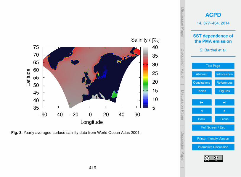
ACPD14, 377–434, 2014


S. Barthel et al.

Title Page



Tables Figures

J I

J I

Back Close

Full Screen / Esc



Discussion

Paper

|D

iscussionP

aper|

Discussion

Paper

|D

iscussionP

aper|


Table 2. Geographical position of the stations used for model eval-uation

Station Country Latitude Longitude

Virolahti II Finland 60.527◦N 27.686◦EBirkenes Norway 58.383◦N 8.25◦E

Auchencorth Moss Great Britain 55.793◦N 3.245◦WCabauw Nertherlands 51.97◦N 4.93◦EMelpitz Germany 51.53◦N 12.93◦E

Sao Vincente Cape Vede 16.864◦N 24.417◦W

tion and scavenging efficiencies are used (Tsyro and Erdman,505

2000).

3.3 Hygroscopic growth

The aerosols are treated as dry particles in the model. Butsince SS is hygroscopic and can growth up to four timeslarger in saturated air compared to the dry size (Monahan510

et al., 1986), wet particle sizes must be used for the calcula-tion of the transport processes. For the calculation of the wetsize of PMA the addition of water should be done accountingfor both, SS and OM. The knowledge about the compositionof OM is still incomplete (Gantt and Meskhidze, 2013). It515

has been found that it can be either hydrophilic or hydropho-bic (Maria et al., 2004). Here, the influence of OM on wa-ter uptake is neglected resulting in the water uptake of theaerosols occurring only due to the SS. For the calculation ofthe growth of SSA we use the volume form of an equation by520

Lewis and Schwartz (2006):

VwetVdry

=

(4

3.7

)3

· 2−RH1−RH

, (15)

where RH is the relative humidity. Thus the water uptakeby the aerosols is a diagnostic variable in the model, calcu-lated at every time step.525

Since the model transports aerosol masses, the densi-ties are taken as 2165kgm−3 for SS (Keene et al., 2007),1300kgm−3 for the OM and 1000kgm−3 for water.

3.4 Observational data

The model results from this work are compared to measure-530

ments from the EMEP monitoring network during the twointensive measurement campaigns in June 2006 and January2007. The stations Birkenes (NO), Melpitz (GER), Virolahti(FI) (Tsyro et al., 2011; Yttri et al., 2008) as well as Auchen-corth Moss (GB) and Cabauw (NL) representing different535

locations have been chosen for the comparison (Tab. 2).Auchencorth Moss near the east coast of Scotland has strongmarine influence mainly from the Atlantic. During westernwinds some of the marine aerosol particles are deposited onthe island, comparably to the stations Cabauw in the Nether-540

lands and Birkenes in southeast Norway. They are strongly

Fig. 3. Yearly averaged surface salinity data from World OceanAtlas 2001

influenced by marine air but located inland. Some particlescan be removed before the air reaches the measurement sites.A further marine station is Virolahti II in southeast Finland,which is influenced by PMA from the low salinity Baltic Sea.545

The continental station Melpitz (Germany) represents long-range transport of PMA and is strongly impacted by deposi-tion. These stations are equipped with filter pack, high- andlow volume samplers and/or MARGA (Monitor for Aerosolsand Gases in ambient Air) with additional chemical analysis550

at a height of 2m. Mass concentrations for PM1, PM2.5 andPM10 are determined daily. To trace SS the sodium concen-tration within the observed aerosol is used, which has onlyminor anthropogenic sources (Tsyro et al., 2011). For theconversion from SS to sodium mass a factor of 0.3061 is used555

(Seinfeld and Pandis, 2006).While the EMEP stations represent the mid latitudes with

lower SST, the measurements from the Cape Verde Atmo-spheric Observatory (CVAO) at Sao Vincente (Tab. 2) rep-resent a region with higher SST. This island lays within the560

Cape Verde archipelago 700km west of Africa. Its aerosolcomposition is dominated by mineral dust from the Sa-hara, biomass burning aerosol and aerosols of marine origin(Heinold et al., 2011; Muller et al., 2010, 2011). The mea-surements used here were obtained with a 5-stage Berner-565

impactor mounted at the top of a 30 meter high tower 70m in-land off the coast to avoid direct influence by sea spray. Thestages of this impactor were separated into: stage 1: 0.05−0.14µm, stage 2: 0.14− 0.45µm, stage 3: 0.45− 1.2µm,stage 4: 1.2−3.5µm, stage 5: 3.5−10µm. (Muller et al.,570

2010). The measurements used here have a daily frequencyand were obtained in December 2007.

3.5 Description of case study and model setup

Three model simulations were carried out to capture all threemeasurement periods. For the comparison with the EMEP-575

stations in June 2006 and January 2007 an European region

Fig. 3. Yearly averaged surface salinity data from World Ocean Atlas 2001.

419





ACPD14, 377–434, 2014


S. Barthel et al.

Title Page



Tables Figures

J I

J I

Back Close

Full Screen / Esc



Discussion

Paper

|D

iscussionP

aper|

Discussion

Paper

|D

iscussionP

aper|

8 Barthel et al.: SST dependence of the PMA emission

Fig. 4. Monthly averaged surface chlorophyll-a concentra-tion merged and interpolated from MODIS-AQUA and MODIS-TERRA data for December 2007

(Fig. 3) including the north east Atlantic as potential sourcefor PMA was chosen. The model uses a horizontal grid reso-lution of 0.25◦ and 30 vertical model layers in MUSCAT and40 layers in COSMO. The mid-height of the lowest level is580

at approximately 10m. The spin up time of the model is fivedays.

For the comparison to the measurements at Sao Vincentein December 2007 a second model domain is used (Africandomain) (Fig. 4). The grid resolution is the same as for the585

European domain except that z1/2 = 33m, which is close tothe measurement height of the tower.

Further input data needed for the simulation of PMA emis-sion are visualised in Fig. 3 and 4. Ocean surface salinitydistribution is shown in Fig. 3 for the ”European” domain.590

There, the yearly averaged values from the World Ocean At-las 2001 at 0.25◦ grid resolution are taken.

The simulation of the fraction of OM within PMA requiresthe sea surface chlorophyll-a concentration fields. Satelliteretrievals provide the best spatial coverage. The chlorophyll595

product from MODIS-Aqua and MODIS-Terra were takenfrom the OceanColour webpage. Here, the averages of themonthly mean values of both satellites were used. Missingdata points were filled with the climatological monthly meanvalues. Remaining gaps were filled by linear interpolation600

(Fig. 4).To take the influence of the SST on the PMA emission

fluxes into account, SST data fields are needed. These weretaken from COSMO based on the reanalysed input data ofthe GME model.605

4 Model results

Since the emission flux and the vertical transport of PMAby turbulence are very sensitive to the surface wind speed itis important that the model reproduces this parameter real-

Fig. 5. Modelled first layer wind speed compared to measure-ments made during an Atlantic transsec (Cape Town towards Bre-merhaven) with the research vessel Polarstern between 28.4.2011and 17.5.2011 compared to the 1:1 line

istically. Modelled surface wind speeds were compared to610

measurements made during the northward-directed Atlantictransec cruise number ANT-XXVII/4 of the research ves-sel Polarstern. The measurements of the wind speed at thePolarstern were made at 37m-height above sea level, whichis approximately the half level height of the lowest level of615

the ”African” domain. The model first layer wind speedsare plotted against these observations in Fig. 5. The modelslightly underestimates the measured wind speeds. The slopeof the regression between model and observations is 0.8(R2 = 0.68). This implies that the model slightly underes-620

timates PMA emission fluxes, due to the wind speed depen-dence. This would be partly compensated by an overesti-mated wind speed dependence in the PMA-emission flux pa-rameterisation by Long et al. (2011). There the authors as-sumed all air, which is entrained into the ocean, detrains as625

bubbles. As mentioned above, a part of the air dissolves inthe ocean during the raise back to the surface leading to alower amount of air detraining by bubbles than entrained bywave breaking.

4.1 Comparison of modelled sea salt aerosol with sta-630

tion data

The model results for sodium concentrations were comparedwith the measurements from the two EMEP-intensive cam-paigns in January 2007 and June 2006 (Fig. 6 to 8). Themeasurements (black symbols) are shown together with the635

model results neglecting a SST-dependence (blue lines) andusing the S11-SST-correction (red lines). In all figures theEMEP-stations are sorted from north to south for January2007 and June 2006.

To compare the model results for coarse mode particles,640

PM10-PM2.5 were calculated from PM10 and PM2.5 data(Fig. 6). It should be noted that the measurement uncertain-

Fig. 4. Monthly averaged surface chlorophyll a concentration merged and interpolated fromMODIS-AQUA and MODIS-TERRA data for December 2007.

420





ACPD14, 377–434, 2014


S. Barthel et al.

Title Page



Tables Figures

J I

J I

Back Close

Full Screen / Esc



Discussion

Paper

|D

iscussionP

aper|

Discussion

Paper

|D

iscussionP

aper|


Fig. 4. Monthly averaged surface chlorophyll-a concentra-tion merged and interpolated from MODIS-AQUA and MODIS-TERRA data for December 2007

(Fig. 3) including the north east Atlantic as potential sourcefor PMA was chosen. The model uses a horizontal grid reso-lution of 0.25◦ and 30 vertical model layers in MUSCAT and40 layers in COSMO. The mid-height of the lowest level is580

at approximately 10m. The spin up time of the model is fivedays.

For the comparison to the measurements at Sao Vincentein December 2007 a second model domain is used (Africandomain) (Fig. 4). The grid resolution is the same as for the585

European domain except that z1/2 = 33m, which is close tothe measurement height of the tower.

Further input data needed for the simulation of PMA emis-sion are visualised in Fig. 3 and 4. Ocean surface salinitydistribution is shown in Fig. 3 for the ”European” domain.590

There, the yearly averaged values from the World Ocean At-las 2001 at 0.25◦ grid resolution are taken.

The simulation of the fraction of OM within PMA requiresthe sea surface chlorophyll-a concentration fields. Satelliteretrievals provide the best spatial coverage. The chlorophyll595

product from MODIS-Aqua and MODIS-Terra were takenfrom the OceanColour webpage. Here, the averages of themonthly mean values of both satellites were used. Missingdata points were filled with the climatological monthly meanvalues. Remaining gaps were filled by linear interpolation600

(Fig. 4).To take the influence of the SST on the PMA emission

fluxes into account, SST data fields are needed. These weretaken from COSMO based on the reanalysed input data ofthe GME model.605

4 Model results

Since the emission flux and the vertical transport of PMAby turbulence are very sensitive to the surface wind speed itis important that the model reproduces this parameter real-

Fig. 5. Modelled first layer wind speed compared to measure-ments made during an Atlantic transsec (Cape Town towards Bre-merhaven) with the research vessel Polarstern between 28.4.2011and 17.5.2011 compared to the 1:1 line

istically. Modelled surface wind speeds were compared to610

measurements made during the northward-directed Atlantictransec cruise number ANT-XXVII/4 of the research ves-sel Polarstern. The measurements of the wind speed at thePolarstern were made at 37m-height above sea level, whichis approximately the half level height of the lowest level of615

the ”African” domain. The model first layer wind speedsare plotted against these observations in Fig. 5. The modelslightly underestimates the measured wind speeds. The slopeof the regression between model and observations is 0.8(R2 = 0.68). This implies that the model slightly underes-620

timates PMA emission fluxes, due to the wind speed depen-dence. This would be partly compensated by an overesti-mated wind speed dependence in the PMA-emission flux pa-rameterisation by Long et al. (2011). There the authors as-sumed all air, which is entrained into the ocean, detrains as625

bubbles. As mentioned above, a part of the air dissolves inthe ocean during the raise back to the surface leading to alower amount of air detraining by bubbles than entrained bywave breaking.

4.1 Comparison of modelled sea salt aerosol with sta-630

tion data

The model results for sodium concentrations were comparedwith the measurements from the two EMEP-intensive cam-paigns in January 2007 and June 2006 (Fig. 6 to 8). Themeasurements (black symbols) are shown together with the635

model results neglecting a SST-dependence (blue lines) andusing the S11-SST-correction (red lines). In all figures theEMEP-stations are sorted from north to south for January2007 and June 2006.

To compare the model results for coarse mode particles,640

PM10-PM2.5 were calculated from PM10 and PM2.5 data(Fig. 6). It should be noted that the measurement uncertain-

Fig. 5. Modelled first layer wind speed compared to measurements made during an Atlantictranssec (Cape Town towards Bremerhaven) with the research vessel Polarstern between 28April 2011 and 17 May 2011 compared to the 1 : 1 line.

421





ACPD14, 377–434, 2014


S. Barthel et al.

Title Page



Tables Figures

J I

J I

Back Close

Full Screen / Esc



Discussion

Paper

|D

iscussionP

aper|

Discussion

Paper

|D

iscussionP

aper|


Fig. 6. Modelled PM10-PM2.5 sodium mass concentration withoutSST correction (blue lines) and with SST correction using S11 (redlines) compared to EMEP measurements (black symbols)

ties of PM10-PM2.5 thus contain the uncertainties of bothmeasurements. PM10-PM2.5 measurements data show 2−3times higher sodium concentrations at Auchencorth Moss,645

Cabauw and Melpitz in winter compared to summer. Thiscan be attributed to the higher wintertime wind speed (Tsyroet al., 2011), which is the dominating parameter for PMAemissions. The salting of icy roads may also have an influ-

Fig. 7. Modelled PM2.5 sodium mass concentration without SSTcorrection (blue lines) and with SST correction using S11 (red lines)compared to EMEP measurements (black symbols)

ence on the wintertime measurements, but is assumed to be650

of less importance (Tsyro et al., 2011). The measured sodiumconcentration at Virolahti is by a factor of 0.7 lower in Jan-uary compared to June. This points to the importance of SST,which varies strongly in the Baltic Sea (near Virolahti) byup to a factor of 6 between January and June. At other sta-655

tions it varies only by 1.8 (Irish Sea) to 3.2 (German Bay).

Fig. 6. Modelled PM10–PM2.5 sodium mass concentration without SST correction (blue lines)and with SST correction using S11 (red lines) compared to EMEP measurements (black sym-bols).

422





ACPD14, 377–434, 2014


S. Barthel et al.

Title Page



Tables Figures

J I

J I

Back Close

Full Screen / Esc



Discussion

Paper

|D

iscussionP

aper|

Discussion

Paper

|D

iscussionP

aper|


Fig. 6. Modelled PM10-PM2.5 sodium mass concentration withoutSST correction (blue lines) and with SST correction using S11 (redlines) compared to EMEP measurements (black symbols)

ties of PM10-PM2.5 thus contain the uncertainties of bothmeasurements. PM10-PM2.5 measurements data show 2−3times higher sodium concentrations at Auchencorth Moss,645

Cabauw and Melpitz in winter compared to summer. Thiscan be attributed to the higher wintertime wind speed (Tsyroet al., 2011), which is the dominating parameter for PMAemissions. The salting of icy roads may also have an influ-

Fig. 7. Modelled PM2.5 sodium mass concentration without SSTcorrection (blue lines) and with SST correction using S11 (red lines)compared to EMEP measurements (black symbols)

ence on the wintertime measurements, but is assumed to be650

of less importance (Tsyro et al., 2011). The measured sodiumconcentration at Virolahti is by a factor of 0.7 lower in Jan-uary compared to June. This points to the importance of SST,which varies strongly in the Baltic Sea (near Virolahti) byup to a factor of 6 between January and June. At other sta-655

tions it varies only by 1.8 (Irish Sea) to 3.2 (German Bay).

Fig. 7. Modelled PM2.5 sodium mass concentration without SST correction (blue lines) and withSST correction using S11 (red lines) compared to EMEP measurements (black symbols).

423





ACPD14, 377–434, 2014


S. Barthel et al.

Title Page



Tables Figures

J I

J I

Back Close

Full Screen / Esc



Discussion

Paper

|D

iscussionP

aper|

Discussion

Paper

|D

iscussionP

aper|


Fig. 8. Modelled PM1 sodium mass concentration without SSTcorrection (blue lines) and with SST correction using S11 (red lines)compared to EMEP measurements (black symbols)

Near Virolahti the monthly averaged wind speed (model) in-creased by 1.8 from June to January. At Birkenes there isalso a slight decrease by a factor of 0.9 in the sodium con-centration, which is attributed to the different origin of the air660

masses in January and June. In January the main wind direc-tion is west to northwest, resulting in a long transport timeover land, which leads to a higher amount of particles to bedeposited before they reach the station. In June, the mainwind direction varies in such way that a higher amount of665

particles is advected from south to east, where transport overland is short. The highest monthly averaged sodium con-centrations (0.69µgm−3) are found at Cabauw in January.While the concentrations at Auchencorth Moss are clearlyhigher than at the inland station Melpitz with 0.63µgm−3

670

to 0.4µgm−3 in January, they are nearly equal in June with0.26µgm−3 to 0.2µgm−3. The low sodium concentration(0.15µgm−3 in January and 0.22µgm−3 in June) at Viro-lahti, which is comparable to or lower than at Melpitz, resultsfrom the low salinity of the Baltic Sea impacting PMA at Vi-675

rolahti. In contrast, Melptiz is influenced by air masses fromthe Atlantic Ocean and North Sea. The model results withthe uncorrected SS source function overestimate the concen-tration at nearly all stations and fit only at a few points wellto the measurements. The SST-correction using S11 leads to680

a better agreement between model results and measurementswith a tendency to underestimate the measured concentrationat some points, especially at peak concentrations.

The PM2.5 sodium concentrations in Fig. 7 show compa-rable features to PM10-PM2.5 with higher monthly averaged685

concentrations for Auchencorth Moss (3.0 times), Cabauw(1.8 times) and Melpitz (2.6 times) in winter than in sum-mer. While the monthly average concentration at Virolahti in

June is nearly equal to that in January, at Birkenes the con-centration is by a factor of 3.2 lower in June compared to690

January, which is the highest factor for all 5 stations; and incontrast to PM10-PM2.5 where the wintertime concentrationwere slightly lower. This may be due to the lower depositionvelocities of the smaller particles resulting in higher concen-tration in January, although the air mass travels a longer way695

over land. Once again the highest average concentration isfound at Cabauw with 1µgm−3 in January and the lowestat Virolahti and Melpitz with 0.11µgm−3 and 0.1µgm−3 inJune, whereas Birkenes has also a low concentration in Junewith 0.12µgm−3. In January the concentration at Virolahti700

is the lowest with 0.11µgm−3. Again the SST-correction byS11 decreases the modelled sodium concentration, but lessthan for PM10-PM2.5. The overestimation using the uncor-rected source function is decreased or disappeared at all sta-tions, so the S11 tends to underestimate the sodium concen-705

tration at some points.PM1 concentration data were only available at the stations

Virolahti and Melpitz from January 2007 and June 2006 (Fig.8). At both stations the measured concentrations are lowerin June than in January with 0.77 and 0.87 in the monthly710

averaged values. In both months the sodium concentrationis nearly 4.6 times higher at Melpitz than at Virolahti. Againthis is due to the air mass origin (the low salinity in the BalticSea causing less SS in Virolahti) and the low deposition rateof the small particles, which causes less PM1 removal com-715

pared to PM10 removal. The S11-SST-function lowers thePM1 concentration compared to the uncorrected version.

Figure 9 compares the model results for sodium with mea-surements by a Berner-impactor which operated at Sao Vin-cente. The measured sodium concentration increases from720

the second to the fifth impactor stage. The higher concentra-tion in the first stage compared to the second were found inother measurements at this station as well (compare Muller etal. (2010)) and may be due to higher uncertainties in the mea-surements at these low sodium concentrations. The model725

results with the S11-SST-correction are only a little lowerthan the uncorrected results, which is much less than the dif-ference at the EMEP-stations due to the higher SST in thesubtropical Atlantic (∼ 20◦C). At the second impactor stageboth model versions slightly overestimate the measurements,730

while at the third to fifth stage both fit well, where S11 fitsslightly better.

4.2 Contribution of organic matter to PMA

The contribution of primary OM to PMA is evaluated for the”African” domain in December 2007. This OM is emitted735

from the ocean surface mixed with SS. Figure 10 shows themonthly averaged emission fluxes of organic carbon (OC)obtained with the SST-correction function of S11. A con-version factor of 2 (Muller et al., 2010; Turpin et al., 2000),which stands for aged aerosol, was applied to obtain the OC740

mass from the modelled OM. The total amount of OC is

Fig. 8. Modelled PM1 sodium mass concentration without SST correction (blue lines) and withSST correction using S11 (red lines) compared to EMEP measurements (black symbols).

424





ACPD14, 377–434, 2014


S. Barthel et al.

Title Page



Tables Figures

J I

J I

Back Close

Full Screen / Esc



Discussion

Paper

|D

iscussionP

aper|

Discussion

Paper

|D

iscussionP

aper|


Fig. 9. Modelled sodium mass concentration without SST correction (blue lines) and with SST correction using S11 (red lines) compared tothe Berner-impactor measurements at Sao Vincente (black symbols) for December 2007

found to be up to 3 times higher in the emitted submicron par-ticles than in the supermicron particles. A maximum emis-sion flux of 9ngm−2s−1 was found west of Great Britain. Inthis area high wind speeds often occur, especially in winter-745

time. The OC flux distribution shown in Fig. 10 indicatesthat the distribution of the OC emission is more strongly in-fluenced by the wind speed, due to the correlation to the SSemission flux, than by the chlorophyll-a concentration (com-pare Fig. 4). An inversely proportional wind speed depen-750

dence of the RV p ratio, due to stronger ocean surface mix-ing and surface microlayer destruction at higher wind speeds(Gantt et al., 2011), would lower the influence of the windspeed on the total OC emission rate.

The locally increased emission fluxes west of Africa are755

due to the higher chlorophyll-a concentration, which is a re-sult of the increased primary production supported by highnutrient availability due to upwelling at the African westcoast and the deposition of mineral dust from the Sahara.This region is important for the measurements at Sao Vin-760

cente since the majority of the detected air masses origi-nate there. This leads to the daily averaged contribution ofOM in the total PMA, shown in Fig. 11 for all 5 impactorstages at Sao Vincente. From the second to the fifth stagethe measured RV p decrease from 0.95 to 0.25, which is cap-765

tured by the model. The lower ratio in stage 1 compared tostage 2 can be related to the higher sodium concentration instage 1. Compared to the measurements the modelled RV pshows much less variability at all sizes. This variability isdue to the slightly different origins of the PMA with dif-770

ferent chlorophyll-a concentration. The inclusion of a wind

speed dependence in computation of the contribution of OMto total PMA and the use of daily resolved chlorophyll-a con-centration instead of the monthly averaged values may causehigher variability in the modelled RV p. The comparison of775

the model results with the measurements shows that the pa-rameterisation of Long et al. (2011) in the current setup re-trieves OM volume ratios, which underestimate the measure-ments at the four larger impactor stages. Likely this underes-timation is a result of underestimating the total OM concen-780

tration, since the sodium concentration is in good agreementwith the measurements (Fig. 9). This seems to be in contrastto the results of Gantt et al. (2012b), who found the param-eterisation by Long et al. (2011) overpredicts the concentra-tion of OM at Mace Head (53.33◦N, 9.90◦W) and Amster-785

dam Island (37,80◦S, 77.57◦E). However, those results werecompared to stations in the mid-latitudes, while here the re-sults are compared to a station in the lower latitudes (Tab. 2).Also, the model assumptions differ from each other, so thatthe results are not directly comparable. The differing results790

highlight the importance of the model set up to account forthe correct description of the emission rates.

4.3 Emission fluxes

For the two simulations in January 2007 and June 2006 themonthly averaged emission fluxes of dry submicron and su-795

permicron PMA mass are plotted in Fig. 12. There the re-sults without temperature correction are shown. Due to thehigher wind speeds in winter especially over the Atlantic theemission rates as well as the maximum emissions are higherin January than in June, resulting in higher airborne particle800

Fig. 9. Modelled sodium mass concentration without SST correction (blue lines) and with SSTcorrection using S11 (red lines) compared to the Berner-impactor measurements at Sao Vin-cente (black symbols) for December 2007.

425





ACPD14, 377–434, 2014


S. Barthel et al.

Title Page



Tables Figures

J I

J I

Back Close

Full Screen / Esc



Discussion

Paper

|D

iscussionP

aper|

Discussion

Paper

|D

iscussionP

aper|


Fig. 10. Modelled monthly averaged emission fluxes of organic carbon for December 2007

Fig. 11. Modelled RV p = VOM/Vp in the aerosol phase compared to measurements with a Berner-impactor at Sao Vincente (Cape Verde)

concentrations. This model result reproduces the majorityof the measurements (compare Fig. 6 and 7). The locationof the highest emission rates differs between January andJune as well. While in June the areas with the local maxi-mal emission rates are located north west of Ireland and west805

of Iceland, in January the maximum emission is spread overa larger area west of Ireland and Scotland with additionalstrong emissions from the North Sea. The low emission ratesat the Baltic Sea are due its low salinity.

The SST correction factors applied to the emission fluxes810

are recalculated from the monthly averaged total emissionfluxes for submicron and for supermicron particles (Figs.13-14). The factors for all size classes differ more or lessstrongly from each other with the majority retrieving a factorlower than 1, thus decreasing the emission rates. The emis-815

sion fluxes of supermicron particles are decreased by all pa-

rameterisations. The strongest decrease was found for S11,while the highest correction factors are found for the Zb13starting north of Great Britain, because the emissions wereunaffected above TW = 13◦C in that parameterisation. Apart820

from reducing emissions, none of the correction functionschanges the regional characteristics of the emission fluxes,which remains dominated by the wind speed. J11 and S11show the same characteristics in the submicron size frac-tion of PMA. The correction factor from J11 is identical for825

the submicron and supermicron particles, due to the missingsize dependence. The submicron correction factor for S11 ishigher than for supermicron particles but still below 1. Thisis despite the fact that the S11-function showed an increasein the emission rates of small particles (see Fig. 1). However,830

since it decreases emissions for particles larger than 0.2µmwhich dominate the mass of submicron particles this leads

Fig. 10. Modelled monthly averaged emission fluxes of organic carbon for December 2007.

426





ACPD14, 377–434, 2014


S. Barthel et al.

Title Page



Tables Figures

J I

J I

Back Close

Full Screen / Esc



Discussion

Paper

|D

iscussionP

aper|

Discussion

Paper

|D

iscussionP

aper|


Fig. 10. Modelled monthly averaged emission fluxes of organic carbon for December 2007

Fig. 11. Modelled RV p = VOM/Vp in the aerosol phase compared to measurements with a Berner-impactor at Sao Vincente (Cape Verde)

concentrations. This model result reproduces the majorityof the measurements (compare Fig. 6 and 7). The locationof the highest emission rates differs between January andJune as well. While in June the areas with the local maxi-mal emission rates are located north west of Ireland and west805

of Iceland, in January the maximum emission is spread overa larger area west of Ireland and Scotland with additionalstrong emissions from the North Sea. The low emission ratesat the Baltic Sea are due its low salinity.

The SST correction factors applied to the emission fluxes810

are recalculated from the monthly averaged total emissionfluxes for submicron and for supermicron particles (Figs.13-14). The factors for all size classes differ more or lessstrongly from each other with the majority retrieving a factorlower than 1, thus decreasing the emission rates. The emis-815

sion fluxes of supermicron particles are decreased by all pa-

rameterisations. The strongest decrease was found for S11,while the highest correction factors are found for the Zb13starting north of Great Britain, because the emissions wereunaffected above TW = 13◦C in that parameterisation. Apart820

from reducing emissions, none of the correction functionschanges the regional characteristics of the emission fluxes,which remains dominated by the wind speed. J11 and S11show the same characteristics in the submicron size frac-tion of PMA. The correction factor from J11 is identical for825

the submicron and supermicron particles, due to the missingsize dependence. The submicron correction factor for S11 ishigher than for supermicron particles but still below 1. Thisis despite the fact that the S11-function showed an increasein the emission rates of small particles (see Fig. 1). However,830

since it decreases emissions for particles larger than 0.2µmwhich dominate the mass of submicron particles this leads

Fig. 11. Modelled RVp = VOM/Vp in the aerosol phase compared to measurements witha Berner-impactor at Sao Vincente (Cape Verde).

427





ACPD14, 377–434, 2014


S. Barthel et al.

Title Page



Tables Figures

J I

J I

Back Close

Full Screen / Esc



Discussion

Paper

|D

iscussionP

aper|

Discussion

Paper

|D

iscussionP

aper|


Fig. 12. Monthly averaged total PMA mass emission fluxes for submicron (top panels) and super micron (bottom panels) PMA emission inJanuary 2007 (left panels) and June 2006 (right panels)

Fig. 13. Monthly averaged SST-correction factors for submicron PMA emission in June 2006 (top panels) and January 2007 (bottom panels)for the different parameterizations

Fig. 12. Monthly averaged total PMA mass emission fluxes for submicron (top panels) andsuper micron (bottom panels) PMA emission in January 2007 (left panels) and June 2006 (rightpanels).

428





ACPD14, 377–434, 2014


S. Barthel et al.

Title Page



Tables Figures

J I

J I

Back Close

Full Screen / Esc



Discussion

Paper

|D

iscussionP

aper|

Discussion

Paper

|D

iscussionP

aper|


Fig. 12. Monthly averaged total PMA mass emission fluxes for submicron (top panels) and super micron (bottom panels) PMA emission inJanuary 2007 (left panels) and June 2006 (right panels)

Fig. 13. Monthly averaged SST-correction factors for submicron PMA emission in June 2006 (top panels) and January 2007 (bottom panels)for the different parameterizations

Fig. 13. Monthly averaged SST-correction factors for submicron PMA emission in June 2006(top panels) and January 2007 (bottom panels) for the different parameterizations.

429





ACPD14, 377–434, 2014


S. Barthel et al.

Title Page



Tables Figures

J I

J I

Back Close

Full Screen / Esc



Discussion

Paper

|D

iscussionP

aper|

Discussion

Paper

|D

iscussionP

aper|


Fig. 14. Monthly averaged SST-correction factors for supermicron PMA emission in June 2006 (top panels) and January 2007 (bottompanels) for the different parameterizations

to the decrease of the total emission fluxes with temperature.Finally the Zb13-correction function increases the submicronemissions for lower SST. This is because of the high factor835

for particles around 0.1 micron, which then dominate the sizedistribution. This high factor leads to changed regional char-acteristics of the highest PMA emission rates, which are nowlocated at the low temperature water around Greenland. Fur-thermore the high correction factors at the northern Baltic840

Sea should be noted, which lead to strong increases in theemission rates resulting in high concentrations at Virolahtiwhen using this function.

4.4 Sensivity to correction of the SST

The Figs. 15-18 show boxplots with the 5, 25, 50, 75 and 95-845

percentile for the measurements compered to the median ofthe model results, where S11 is given in red symbols, J11 inblack symbols, Zb13 in green symbols and the results with-out SST correction in blue symbols. The daily average val-ues are used for all included data and only these model values850

were taken into account where measurements exist.

4.4.1 PM10-PM2.5

For PM10-2.5 concentrations the measurements and modelresults at the five EMEP-stations are plotted in Fig. 15. Asexplained above, the model simulates the highest sodium855

concentrations when using no correction for SST. All SST-correction functions lower the modelled concentrations, with

Zb13 resulting in the highest and S11 the lowest values.The uncorrected values are higher than the measured onesat all stations and higher or even near the 95-percentile at860

the majority of the stations especially in January. For Vi-rolahti, Birkenes and Melpitz in June the uncorrected con-centrations are closer to the measured median and within the75-percentile. The higher overprediction in January pointstowards the need of the SST correction. All three tested cor-865

rection functions improved the model results compared to themeasurements. While Zb13 and J11 lower the concentrationsonly a little so that there are still stations with overpredictionof sodium concentrations, the S11-function lead to underes-timations of the modelled concentrations except at Auchen-870

corth Moss and Birkenes in January, but overall the S11-SST-correction result in the best agreement of model results andobservations.

4.4.2 PM2.5

Boxplots of PM2.5 are shown for the same stations as for875

PM10-PM2.5 (Fig. 16). In that size range no clear opti-mum correction function is found. The Zb13-function in-creases the concentrations, because the correction factor ishigher than 1 for particles smaller than 1.8µm. This leads toworse results where the uncorrected version overpredicts the880

measured concentration, but improves the results at Cabauw,Auchencorth Moss in January and Melpitz in June. Since theresults of the uncorrected model are close to the measure-

Fig. 14. Monthly averaged SST-correction factors for supermicron PMA emission in June 2006(top panels) and January 2007 (bottom panels) for the different parameterizations.

430





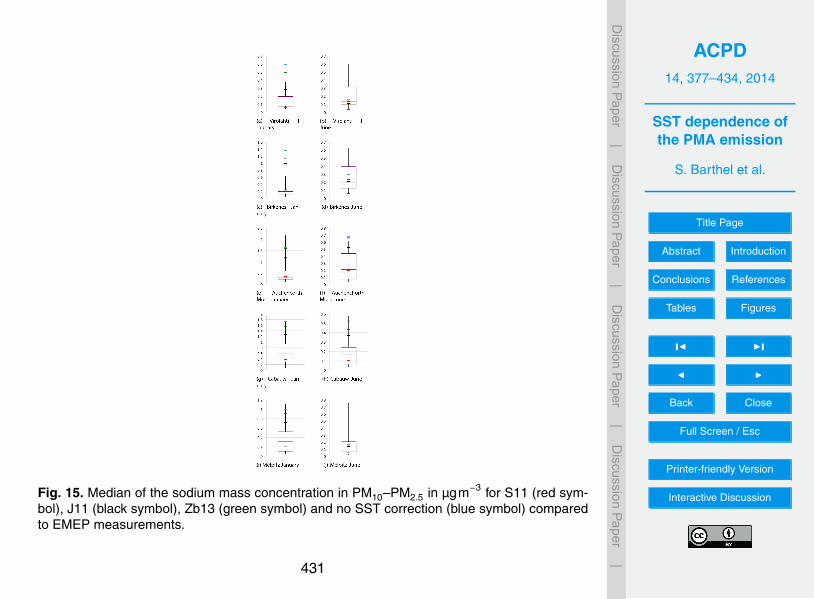
ACPD14, 377–434, 2014


S. Barthel et al.

Title Page



Tables Figures

J I

J I

Back Close

Full Screen / Esc



Discussion

Paper

|D

iscussionP

aper|

Discussion

Paper

|D

iscussionP

aper|


Fig. 15. Median of the sodium mass concentration in PM10-PM2.5in µgm−3 for S11 (red symbol), J11 (black symbol), Zb13 (greensymbol) and no SST correction (blue symbol) compared to EMEPmeasurements

ments, the S11-correction function leads to strong underpre-dictions of the measurements. Overall the J11-function tends885

to result in best agreement with measurements for that casestudy.

4.4.3 PM1

It was mentioned above that the SST-correction with Zb13 re-trieves high correction factors for PM1 at the northern Baltic890

Sea. This leads to high emission rates resulting in high mod-elled concentrations of marine aerosol at the station Viro-lahti. In Fig. 17 it can be seen that these high values leadto a strong overprediction of the sodium mass compared tothe measurements, especially in January. The lower concen-895

trations by the neglection of the SST-dependence or the useof S11 and J11 are closer to the measurements for that sta-tion. However these three model setups underpredicted theconcentration at Melpitz, where the increase of the concen-tration by Zb13 fits best to the measurements.900

4.4.4 Berner-impactor at Sao Vicente

Figure 18 compares the model results with measurements ofa Berner-impactor which operated at the CVAO at Sao Vin-cente. Due to the relatively high SST at these latitudes onlya slight influence by the correction functions can be distin-905

guished. S11 shows the strongest decrease in the concentra-tions, caused by the origin of the air mass, which is mainlyfrom regions with a SST around 20◦C. J11 does not changethe concentrations compared to the uncorrected version sig-nificantly and Zb13 has no influence due to the SST being910

above 13◦C.For the second, fourth and fifth stage best agreement is

for S11, but again with the tendency to underestimate theconcentration. For the third stage it cannot be decided whichparameterisation results in the best values in comparison with915

the measurements.

5 Discussion

The EMEP-intensive campaign measurements were alsoused by Tsyro et al. (2011) for the evaluation of the EMEPchemical transport model. The authors found the model to920

underpredict the PM2.5 and PM10 sodium concentration inJune 2006 while the model underprediction is less or changesto overprediction of the measurements in January 2007. Theyattributed the discrepancies to inaccuracies in the wind pre-diction or the coarse model grid resolution (50x50km−2).925

The same results are found for sodium concentrations forCOSMO-MUSCAT when PMA emissions are not SST cor-rected (Fig. 6 and 7). In contrast to the EMEP-model thesodium concentration is overestimated with the uncorrectedSS source function in COSMO-MUSCAT. SST correction of930

the PMA emission decreases the modelled sodium concen-tration at the EMEP stations, so that the measurements are

Fig. 15. Median of the sodium mass concentration in PM10–PM2.5 in µgm−3 for S11 (red sym-bol), J11 (black symbol), Zb13 (green symbol) and no SST correction (blue symbol) comparedto EMEP measurements.

431





ACPD14, 377–434, 2014


S. Barthel et al.

Title Page



Tables Figures

J I

J I

Back Close

Full Screen / Esc



Discussion

Paper

|D

iscussionP

aper|

Discussion

Paper

|D

iscussionP

aper|


Fig. 16. Median of the sodium mass concentration in PM2.5 inµgm−3 for S11 (red symbol), J11 (black symbol), Zb13 (greensymbol) and no SST correction (blue symbol) compared to EMEPmeasurements

Fig. 17. Median of the sodium mass concentration in PM1 inµgm−3 for S11 (red symbol), J11 (black symbol), Zb13 (greensymbol) and no SST correction (blue symbol) compared to EMEPmeasurements

matched better than without correction. This is particularlyevident for the PM10-PM2.5 size range and for the wintermonth. The strongest emission decrease was obtained by S11935

resulting in underestimation of the sodium concentration atthe measurement sites, while the J11 correction has a smallereffect. For the coarse particles the use of the SST-correctionfunction by S11 gives reasonable results.

The effect of the SST correction is not as clear for PM2.5940

concentrations. For this size range the S11 correction func-tion leads to worse results compared to the other functionsin the comparison with the observations. In the current workthe parameterisation of Long et al. (2011) was used to de-scribe the PMA emission flux. The use of a different PMA945

emission functions (e.g.: Sofiev et al. (2011)) (Fig. 2) withhigher emission rates will result in higher non-SST-correctedPM2.5 sodium concentrations than with the parameteriza-tion by Long et al. (2011). In combination with the S11-SST-correction those modelled concentrations would result950

in better agreement with the observations at the EMEP mea-surement sites, but would lead to overestimations of the con-centrations at Sao Vincente.

At Melpitz, the measured sodium concentrations in thePM1 size range decrease in January compared to June. This955

is in contrast to coarse particles, where they increase. Thisbehaviour is similar for Virolahti, but less clear. Such aneffect could be due to the decrease of the concentration oflarger particles within the size spectrum being partly com-pensated by the increase of smaller particles with lower960

Fig. 16. Median of the sodium mass concentration in PM2.5 in µgm−3 for S11 (red symbol), J11(black symbol), Zb13 (green symbol) and no SST correction (blue symbol) compared to EMEPmeasurements.

432





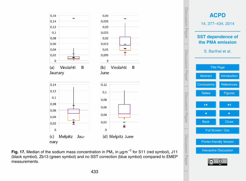
ACPD14, 377–434, 2014


S. Barthel et al.

Title Page



Tables Figures

J I

J I

Back Close

Full Screen / Esc



Discussion

Paper

|D

iscussionP

aper|

Discussion

Paper

|D

iscussionP

aper|


Fig. 16. Median of the sodium mass concentration in PM2.5 inµgm−3 for S11 (red symbol), J11 (black symbol), Zb13 (greensymbol) and no SST correction (blue symbol) compared to EMEPmeasurements

Fig. 17. Median of the sodium mass concentration in PM1 inµgm−3 for S11 (red symbol), J11 (black symbol), Zb13 (greensymbol) and no SST correction (blue symbol) compared to EMEPmeasurements

matched better than without correction. This is particularlyevident for the PM10-PM2.5 size range and for the wintermonth. The strongest emission decrease was obtained by S11935

resulting in underestimation of the sodium concentration atthe measurement sites, while the J11 correction has a smallereffect. For the coarse particles the use of the SST-correctionfunction by S11 gives reasonable results.

The effect of the SST correction is not as clear for PM2.5940

concentrations. For this size range the S11 correction func-tion leads to worse results compared to the other functionsin the comparison with the observations. In the current workthe parameterisation of Long et al. (2011) was used to de-scribe the PMA emission flux. The use of a different PMA945

emission functions (e.g.: Sofiev et al. (2011)) (Fig. 2) withhigher emission rates will result in higher non-SST-correctedPM2.5 sodium concentrations than with the parameteriza-tion by Long et al. (2011). In combination with the S11-SST-correction those modelled concentrations would result950

in better agreement with the observations at the EMEP mea-surement sites, but would lead to overestimations of the con-centrations at Sao Vincente.

At Melpitz, the measured sodium concentrations in thePM1 size range decrease in January compared to June. This955

is in contrast to coarse particles, where they increase. Thisbehaviour is similar for Virolahti, but less clear. Such aneffect could be due to the decrease of the concentration oflarger particles within the size spectrum being partly com-pensated by the increase of smaller particles with lower960

Fig. 17. Median of the sodium mass concentration in PM1 in µgm−3 for S11 (red symbol), J11(black symbol), Zb13 (green symbol) and no SST correction (blue symbol) compared to EMEPmeasurements.

433





ACPD14, 377–434, 2014


S. Barthel et al.

Title Page



Tables Figures

J I

J I

Back Close

Full Screen / Esc



Discussion

Paper

|D

iscussionP

aper|

Discussion

Paper

|D

iscussionP

aper|


Fig. 18. Sodium mass concentration in µgm−3 for S11 (red symbol), J11 (black symbol), Zb13 (green symbol) and no SST correction (bluesymbol) compared to Berner-impactor measurements (Boxplot) at Sao Vincente

SST. However, the evaluation at only two stations and twomonths is insufficient to obtain statistically meaningful re-sults. In general, the uncorrected version tends to underes-timate the PM1 concentration so that the results with Zb13are in best agreement with the measurements at the EMEP965

station. However, the very high correction factor for lowtemperatures leads to overestimations of the concentrationat near coastal stations in winter as at Virolahti. Based onthe small amount of available measurement data, a final con-clusion for the SST-correction function regarding PM1 is not970

possible.

The measured sodium concentration at Virolahti is lowcompared to Cabauw or Auchencorth Moss, although all sta-tions are of marine background. The reason for this is the airmass origin - Virolahti is influenced by air masses from the975

Baltic Sea, which has a salinity of 7h and lower. In contrast,the air mass arriving at Cabauw and Auchencorth Moss orig-inates from the North Sea and the North-east Atlantic, wherethe salinity is around 35h. The model captures the influenceof salinity on SSA emission well.980

The new SST-correction function that was based on mea-surements by Zabori et al. (2012) did not lead to better resultscompared to the other parameterizations. With that parame-terization the concentrations of fine particles were overpre-dicted especially near cold waters, and the decrease of the985

coarse particle concentration was too low to reproduce themeasured concentration. The size dependence of the cor-rection factor cannot be validated by the available measure-ments.

The modelled monthly averaged emission fluxes of submi-990

cron primary OC for the ”African” model domain in Decem-ber 2007 were found to be between 1− 2ngm−2s−1 westof Africa and the Mediterranean Sea and increase west ofEurope towards 9ngm−2s−1 west of Great Britain. This iscomparable to the multi-year average values determined by995

Long et al. (2011) and Spracklen et al. (2008).

6 Conclusions

In this work we tested the importance of considering the in-fluence of SST on PMA emissions, together with impactsof surface winds and salinity. In particular for coarse mode1000

particles neglecting the SST-dependence lead to overestima-tions of the PMA-concentrations by the model compared tomeasurements at land and island stations. While we find thatusing the correction functions by S11 and J11 improve themodel performance for coarse mode particles, not enough1005

data were available for PM1 to test the role of SST in thissize fraction. More measurements in this size range are re-quired to study particle fluxes in the small sizes that are alsoimportant to study the role of PMA in cloud modification.

A size shift of the dry SS size distribution towards smaller1010

sizes with lower salinities could be indicated.For the description of the contribution of OM to PMA a re-

placement of SS by this OM has been assumed in the combi-nation with the Long et al. (2011) function for the descriptionof the their relation to each other. While the monthly aver-1015

aged emission rates for submicron OM in December 2007were found to be comparable to multi-year averaged valuesfrom literature, the measured ratio of OM to total PMA wereunderestimated at Sao Vincente. Since the used parameter-ization was developed from laboratory measurements it ac-1020

counts only for primary OM. However secondary OM mayalso be part of the detected aerosols, leading to underestima-tions by the model results. Furthermore OM from the Africancontinent can be detected within the measurements, whichhas also not been taken into account in the model. Both fac-1025

tors need to be discussed in future works.

Acknowledgements. This work was supported by the German Sci-ence Foundation (DFG) (Grant No. TG 376/6-1) and by the BMBF(Bundesministerium fur Bildung und Forschung) as part of the SO-PRAN project (FZK 03F0611J) which is a German national contri-1030

bution to the international SOLAS project.

Special thanks to the NASA for providing the chlorophyll-adatabase on the OceanColor webpage and NOAA for the salinitydatabase as part of the World Ocean Atlas 2001.

Fig. 18. Sodium mass concentration in µgm−3 for S11 (red symbol), J11 (black symbol), Zb13(green symbol) and no SST correction (blue symbol) compared to Berner-impactor measure-ments (Boxplot) at Sao Vincente.

434





sst dependence of the pma emission - atmos-chem-phys ... fileacpd 14, 377–434, 2014 sst dependence...

Documents