ssib and its sensitivity to soil properties a case study

ELSEVIER Global and Planetary Change 13 (1996) 183-194

GLOBAL AND PLANETARY CHANGE

SSiB and its sensitivity to soil properties a case study using HAPEX-Mobilhy data

Yongkang Xue a Fanl'ong J. Zeng a, C. Adam Schlosser b a Center for Ocean-Land-Atmosphere Studies, 4041 Powder Mill Road, Suite 302, Calverton, MD 20705, USA

b Geophysical Fluid Dynamics Laboratory, Princeton, NJ 08645, USA

Received 5 May 1995; accepted 28 August 1995

Abstract

In this paper, SSiB's development and some of its major parameterizations in the model are briefly reviewed. The soil moisture parameterizations, which are a key element in the model, are comprehensively described.

The sensitivity study shows that hydraulic conductivity at saturation, B parameter, and wilting point have a profound impact on the simulation of soil moisture, hut with different features. Both hydraulic conductivity at saturation and B parameter influence the soil moisture simulation by changing the soil hydraulic conductivity and the field capacity. The changes in equilibrium soil water content in this study are consistent with the changes in field capacity. The wilting point affects the soil moisture through vegetation transpiration.

Through these sensitivity studies, improvements in modeling the soil moisture content of HAPEX-Mobilhy data are made. The soil moisture simulations at six Russian sites are also re-examined. After applying the results from the sensitivity studies of the HAPEX-Mobilhy data, the soil moisture simulation of the Russian data is significantly improved.

1. In t roduc t ion

The SSiB biosphere model (Xue et al., 1991) used in this study is a simplified version of the Simple Biosphere Model (SiB) (Sellers et al., 1986), The vegetation-soil layer affects the radiative transfer at the surface, the partitioning of surface energy into sensible heat flux and latent heat flux. SSiB is intended to realistically simulate the biophysical exchange processes. The biophysical controls on these exchange processes are mutually consistent by modeling the vegetation explicitly. The biosphere model is linked to a general circulation model (GCM) of the atmosphere through fluxes of radiation, sensible and latent heat, and momentum. A coupled biosphere m o d e l - G C M has been shown to be an improvement

over the " b u c k e t " model for simulations of the hydrologic cycle and the surface energy partition (Sato et al., 1989).

To apply the coupled biosphere m o d e l - G C M for extended-range prediction and climate studies, we reduced vegetation and soil parameters from SiB. The values of many of the parameters are scarce for different biomes in different parts of the world. Large number of parameters with only approxi- mately known values would make the sensitivity testing and model validation difficult. Our studies found some vegetation and soil parameters have little effects in the long term GCM simulations. We also used one canopy layer in the SSiB. The multilayer model is more realistic and might be easier to com- pare with the observations over a single site, but it

0921-8181//96/$15.00 © 1996 Elsevier Science B.V. All rights reserved SSDI 0921-81 8 1(95)00045-3

184 Yongkan Xue et al. / Global arm Planetary Change 13 (1996) 183-194

requires more parameters and computer time, and it is not easy to connect its parameters with the satellite observation. A systematic bias in simulated African climate using a coupled SiB-GCM might be due to the difficulty in adequately simulating the interac- tions between different vegetation layers and between the soil and ground vegetation cover (Miyakoda, pers. comm.).

The basic prognostic equations of SSiB and some of its parameterizations will be presented in section 2. SSiB has been implemented in the Center for Ocean-Land-Atmosphere Studies (COLA) GCM and other GCMs and regional models. Using the coupled biosphere-atmosphere model, sensitivity studies have been conducted to test the roles of the desertification in the Sahel on the African drought (Xue and Shukla, 1993a; Xue and Shukla, 1993b), the impact of the desertification over the Inner- Mongolian grassland on the East Asian summer monsoon (Xue, 1995), and the influence of the seasonal variations of crop parameters on the U.S. summer weather prediction (Xue et al., 1996b; Fen- nessy and Xue, 1994). These studies show that changes in the energy budget and hydrological cycle at the surface have a significant impact on regional climate simulations, and that land surface degrada- tion in some areas may be responsible for the decadal climate anomaly over the region. To more realistically assess such an impact, validation and calibra- tion studies of the biosphere model using observed data are necessary.

SSiB's development is based upon observational data from the Amazonian rainforest (Xue et al., 1991). Since then, a number of observational data from different sites and vegetation types are available and have been used to validate and evaluate this model, which include data from the Anglo-Brazilian Amazonian Climate Observation Study (ABRACOS) - - a field experiment over Amazon deforestation site (Xue et al., 1996a); from the Sahelian Energy Bal- ance experiment (SEBEX)--a field experiment over the semi-arid area (Xue and Allen, 1995); from the First ISLSCP field experiment (FIFE) in Kansas (Chen et al., 1996); from the Russian hydrological measurements (Robock et al., 1995; Schlosser, 1995), and from the Cabauw experiment on a grassland site in the Netherlands (Chen et al., 1995).

In this study, the observational data from

HAPEX-Mobilhy is used to validate and evaluate the model simulations. The results presented by other papers in this special issue show that SSiB is able to produce realistic simulations of surface fluxes. How- ever, the simulations of the soil moisture need to be improved (Shao and Henderson-Sellers, 1996-this issue; Mahfouf et al., 1996-this issue). In this paper, we briefly introduce SSiB in section 2. The sensitivity of the model results to soil properties and the improvement of the model simulations using the HAPEX data are discussed in section 3. Based on these sensitivity studies, the soil moisture simulations using the Russian data are also improved. These results are presented in section 4. The summary is given in Section 5.

2. Simplified SiB model (SSiB)

SSiB has three soil layers and one canopy layer, and eight prognostic variables: soil wetness in the three soil layers; temperatures at the canopy, ground surface and deep soil layers; water stored on the canopy; snow stored on the ground (Fig. 1). The governing equation for canopy temperature T c is based on energy conservation equation.

ate c~-g-, = R~c- H~- ae~ (1)

where Q , Rn~ , He, and AE~ are heat capacity of canopy, net radiation, sensible heat, and latent heat fluxes at the canopy level, respectively. The force-re- store method is used to predict the time variation of the ground temperature Tg~.

Or~s Cgs Ot = Rngs - Hgs - AEgs

2~rCgs (Tg~- Td) T

(2)

where r is the day length, Cg s the effective heat capacity of soil, T a the temperature for deep soil, and Rng s, Hg s, and AEg~ are net radiation, sensible heat, and latent heat fluxes at the ground, respectively. The equation for deep soil temperature T a is

OTd 2¢r C g s ( ~ s - rd) Cd Ot = T1 /~N ' / r ( 3 )

Yongkan Xue et al. / Global and Planetary Change 13 (1996) 183-194 185

The governing equation for the canopy interception water store M c is based on water conservation.

3M c - - = P - O - E w e (4)

at 30 ~ 1

where P, D, and Ewe are the precipitation, water 3t = D 1 drainage rate, and evaporation from the wetted por- tions of the vegetation canopy. The governing equa- 302 1

tion for snow depth M s is 3t = D-~2 [ - Q aMs at = Ps - am + Wf (5)

where Ps, Sin, and Wf are snow fall , snow melt, and

A T M O S P H E R I C S U R F A C E L A Y E R

er

kEc+kEs I

ea

rsurf <

J . . . .

f h. e. ( T gs ) z.../_J- ,~/_./- ,, ,

freezing of water, respectively. In the three soil layers, water movement is described by the finite- difference approximation to the diffusion equations

[ P + Q , 2 - E g s - b i E d c ]

-QI2 + Q23 - - bzEdc ]

(6)

(7)

a 0 3 1 = [ - Q23 - Q 3 - b Edc] (8)

3t ~ 3

Tr

ra

r b

~"~CANOPY~:~T~ ~ T~

r a

IH c + Hg s

Fig. 1. Schematic diagram of SSiB. The transfer pathways for latent and sensible heat flux are shown on the left- and right-hand sides of the

diagram, respectively. T r and T a, and e r and e~ are the air temperatures and specific humidi ty at reference height and within the canopy air space, respectively; T~ and Tg are the canopy and the soil temperatures, respectively; e * (T c) and e*(Tg) are the specific humidi ty at saturation at the canopy and the ground, respectively; r a the aerodynamic resistance between canopy air space and reference height; r b the bulk boundary layer resistance; r c the bulk stomatal resistance; r d aerodynamic resistance between canopy air space and ground; rsoil the bare soil surface resistance. H c and Hg s are the sensible heat flux from canopy and ground, respectively. E c and E s are the latent heat flux from canopy and ground, respectively, fh is the a function to adjust bare soil evaporation.

186 Yongkan Xue et al. / Global and Planetary Change 13 (1996) 183-194

where the 0 1 , 0 2 , 0 3 , D 1, D2, and D 3 are the volumetric soil water content and soil thickness of the top, middle, and lower soil layers, respectively. Edc is the transpiration rate. Eg S is the evaporation from bare soil. bi( i = 1,2,3) is the fraction factor and depends on the root distribution. Qi,j is the transfer of water between ith and jth layers and is defined to be positive upward as

where k is the hydraulic conductivity, 0 is the soil water potential, and z is the thickness between two soil layers. Numerous parameterizations for the soil water retention and hydraulic conductivity functions have been developed over the decades (Van Genuchten, 1980; Brooks and Corey, 1964; Gardner, 1958; Clapp and Hornberger, 1978; Cosby et al., 1984; Ek and Cuenca, 1994). The soil water potential in this model is taken from the empirical relationship of Clapp and Hornberger (1978),

~b= ~b s (10)

where O s is the volumetric soil water content at saturation; the B parameter is an empirical constant dependent on the soil type. The relationship between ~b and B are displayed in Fig. 2a. The drainage of water out of the bottom layer is

Q3 = k3 * s in x + Qb ( 1 1)

The first term of the right hand side of the Eq. (11) is contributed by gravity only, with no diffusive trans- port occurring, as modeled by Sellers et al. (1986). x is the mean slope angle and set to larger than 3 ° and k 3 is the hydraulic conductivity at the third layer. Qb is the base flow runoff and proportional to the soil wetness in the lower soil layer, Qb = Kc *(03/0s)- 03 is the volumetric soil water content at the third soil layer. This term is suggested by Liston et al. (1994) to account for the GCM grid-box spatial variation of the soil moisture. The empirical constant Ko is derived from large river basins. The hydraulic conductivity at layer i, k i, is

k i = k s ( O i / / O s ) (2B+3) ( 1 2 )

14-

"~ 8- Q._

I 6

2 J 0

-2 -4

0 - 5 - -

-~0 -15

~ -20 -25

-30

-35

-4(1

(3 4 5 6 7 8 9 10 1 1 t2

13 parameter

3

0

4 ~ 6 7 8 9 10 11 12

B parameter

- 5

- I 0 ,

~ " -15.

~ " -20"

-25

-30.

-35

-40 • C

- 7 - 6 -,5 - 4 - 3

LOG(Ks) -2

Fig. 2. Relationship between (a) logarithm of absolute soil water potential and B parameter; (b) logarithm of hydraulic conductivity and B parameter; (c) logarithm of hydraulic conductivity and hydraulic conductivity at saturation. Symbols (3 :0 = 0.05; O: 0=0.1; [2: 0=0.15; 11:0=0.2; +: 0=0.3. No symbol: 0= 0.45. The soil water potential at saturation is - 0.3 and 0 s is 0.45. In (b) k s is 4e-6. In (c) the B is 5.

where k, is the hydraulic conductivity at saturation. Fig. 2b,c shows the relationship between k, and k s and B based on Eq. 12. The logarithm of k reduces linearly as B increases. Hydraulic conductivity changes more dramatically with B in the dry soil than in the wet soil; and has larger variation with soil moisture when B is large. We will discuss these figures further in the next section.

The parameterization of the stomatal resistance, re, in SSiB was based on the work of Jarvis (1976). Three stress terms are included in this scheme which describe the dependence of stomatal resistance to atmospheric temperature, soil water potential, and vapor pressure deficit. Different from the traditional approach in which the leaf water potential was used

Yongkan Xue et al . / Global and Planetary Change 13 (1996) 183-194 187

to calculated the stomatal resistance (Federer, 1979), soil moisture is used to control stomatal resistance in SSiB. Using leaf water potential makes the computa- tion very complex and a large number of parameters are required. Evidence (Blackman and Davies, 1985, Wetzel and Chang, 1987) indicates that stomatal response to water supply is not controlled by the plant's internal water potential. Instead, it appears that roots "sense" the soil moisture supply and directly transmit chemical messages (cytokinin) to the guard cells to keep stomata open. Thus, stomatal closure occurs in direct response to soil moisture and is not delayed while a plant's internal water supply is squandered. The equation of the adjustment factor f(qJ) for soil water potential is

f ( ~ ) = 1 - E X P { - C 2 [ C 1 - l n ( - ~b)]} (13)

where C z depends on the vegetation type and C 1 is a constant, which is obtained using the wilting point. The stomata completely close at the wiling point in the model. C 2 is a slope factor. A large C 2 means that the f(~b) changes from 0 to 1 very fast when soil water content varies from wilting point to the point stomata start to close. Note that in table 1 of Xue et al. (1991) the values of C 1 and C 2 should be interchanged.

The equation for transpiration from canopy is:

(q(Tc) - -qa) E t ( 1 - -we ) (14)

rc + rt,

where the q(T c) and qa are the saturated specific humidity at canopy temperature and specific humidity at the canopy air space, respectively, r b is the bulk boundary layer resistance and r c is the stomatal resistance, w c is the wetness fraction of canopy. Bare soil evaporation in the model is

E s = [ f h q ( T ~ s ) - - q a ] * ( 1 - - gg) (15) Fsurf "[- F d

where the q(Tg s) is the saturated specific humidity at the surface temperature Tg~, and Vg is the vegetation cover. The resistance to the transfer of water vapor from the upper soil layer to the canopy air space includes aerodynamic resistance r d and soil surface resistance rsurf (Fig. 1). The results of Camillo and Gurney (1986) were used to curve-fit a simple rela-

tionship "between soil surface resistance and soil moisture at the first layer.

( rsurf = 101840* 1 ~ Z ] ] (16)

The relative humidity of the air at the soil surface is

¢lg r.R

fh = e (17)

when q*(Tgs)> qa" Otherwise, it equals 1. g is acceleration of gravity and R is the gas constant for water vapor. The parameterizations of the resistance between the reference height and top of the canopy were based upon the similarity theory. A linear relationship between Richardson number and aerodynamic resistance was developed to parameterize the aerodynamic resistance.

3. Model sensitivity to soil properties

Studies have shown that soil properties can have a substantial impact on SSiB's simulations (e.g., Xue et al., 1996a,b). In this study, the HAPEX-Mobilhy data were used to examine the effects of soil properties on the annual cycle simulation of soil moisture, evaporation and sensible heat flux, which have never been investigated in our previous studies due to the limitation in duration and content of the data sets. The observed location is a soya crop field with coniferous forest at Caumont, France. Soya plants start to grow in May and harvest at the end of September. The soil type at Caumont is loam. The vegetation and soil parameters used for the SSiB simulations were provided by this Workshop and will be discussed in detail later.

The results of Soil Workshop Experiment 13, which was a control experiment for the Soil Work- shop, show that SSiB is able to produce reasonable simulations of the heat fluxes (Shao and Henderson- Sellers, 1996-this issue; Mahfouf et al., 1996-this issue). But the simulated total soil water content was too high during the spring and too low during the summer (Fig. 5a). To understand the causes, we performed several sensitivity studies to examine the model 's responses to the variations of soil properties. In this paper, we present the sensitivity of the model

188 Yongkan Xue et al . / Global and Planetary Change 13 (1996) 183-194

simulation to the parameterization of the soil hydraulic properties (k s and B) and the sensitivity to 65o.

6 0 0 - the wilting point. Another soil parameter, soil water E 55o~ potential at saturation @s, has little effect on the ,o 5oo~ simulation when we changed it within a reasonable c~ ~50 range. Its impact will not be discussed in this paper, o ~00

In this study we changed one parameter at a time, = 35o 3OO

and integrated the model for several years by repeat- 2s0 ing the one year of forcing. The results presented here are from the integrations during the second year, when the model simulation had reached equilibrium conditions. Table 1 lists the values of soil ~.i parameters used for Experiments A, B, and C, which changed soil hydraulic conductivity at saturation k s, B parameter, and wilting point, C l, respectively. The changes for each parameter are within the normal

,/A/~ 1 9 8 6 range of soil property variations. For comparison, the 65o

soil parameters for experiment 13 are also listed in 800 the table. E 580

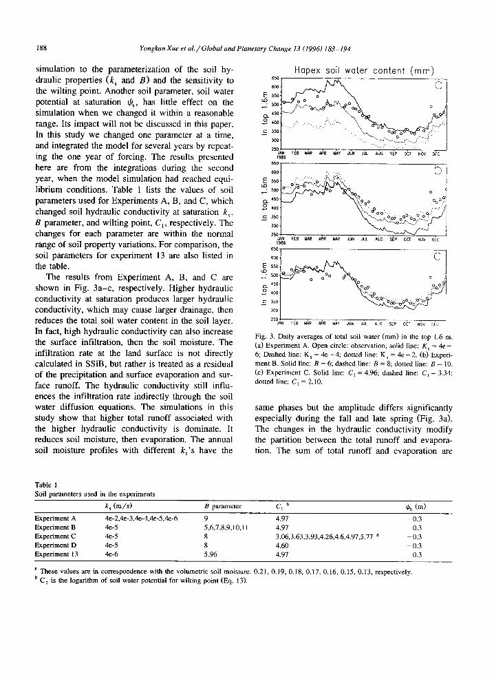
The results from Experiment A, B, and C are ~: 5oo shown in Fig. 3a-c, respectively. Higher hydraulic ~_ ,50

400

conductivity at saturation produces larger hydraulic c 35o conductivity, which may cause larger drainage, then 300 reduces the total soil water content in the soil layer. In fact, high hydraulic conductivity can also increase the surface infiltration, then the soil moisture. The infiltration rate at the land surface is not directly calculated in SSiB, but rather is treated as a residual of the precipitation and surface evaporation and surface runoff. The hydraulic conductivity still influences the infiltration rate indirectly through the soil water diffusion equations. The simulations in this study show that higher total runoff associated with the higher hydraulic conductivity is dominate. It reduces soil moisture, then evaporation. The annual soil moisture profiles with different ks's have the

Hapex soil wa te r c o n t e n t ( m m )

. . i ' . . . : " . ~ , . . ,.~ . o . , . , . , , - " . , . . ,

• . " - , , . , o : - - , . :

• . . . : . . . . . . . . . . .

FEB MAR APR MAY JUN JUL AUG SEP OCT NOV DEC 1986

650

c~ 450 .,..9o0 .% ,,~.~

2,00 - " ~.~.).~Ooo. . . . . .. ~) ..... c 350 "'-- • 6oo" o° 0 .o o :" - - "-,.:,:,, o ~ o ,,---.,.,

,oo

250 . . . . . FEB WIAR APR WAY JUN JUL AUG SEP OCT NOV OEC

C o ~''" ~ o

,Q. =..>~" " o :

o -o 09 :%o:.

250JAN FEB MAR APR MAY JUN JUL AUG SEP OCT NOV DEC

Fig. 3. Daily averages o f total soil water (mm) in the top 1.6 m.

(a) Exper iment A. Open circle: observat ion; solid line: K s = 4 e -

6; Dashed line: K s = 4 e - 4 ; dot ted line: K s = 4 e - 2 . (b) Experi-

men t B. Solid line: B = 6; dashed line: B = 8; dotted line: B = 10.

(c) Exper iment C. Solid line: C l = 4.96; dashed line: C~ = 3.34; dot ted line: C~ = 2.10.

same phases but the amplitude differs significantly especially during the fall and late spring (Fig. 3a). The changes in the hydraulic conductivity modify the partition between the total runoff and evaporation. The sum of total runoff and evaporation are

Table 1 Soil parameters used in the exper iments

k s ( m / s ) B parameter Cl b ~Ps (m)

Exper iment A 4e-2 ,4e-3 ,4e-4 ,4e-5 ,4e-6 9 4.97 - 0.3

Exper iment B 4e-5 5,6,7,8,9,10,11 4.97 - 0.3

Exper iment C 4e-5 8 3 .06,3 .63,3 .93,4 .26,4 .6 ,4 .97,5 .77 a - 0.3 Exper iment D 4e-5 8 4.60 - 0.3

Exper iment 13 4e-6 5.96 4.97 - 0.3

a These values are in cor respondence with the volumetr ic soil moisture: 0 .21, 0 .19, 0.18, 0.17, 0 .16, 0.15, 0.13, respectively. b C l is the logar i thm of soil water potential for wil t ing point (Eq. 13).

Yongkan Xue et al. / Global and Planetary Change 13 (1996) 183-194 1 8 9

650 60O

550 500

E 45o E 4~

~ 350 3OO 25O

+ +

+

x +

×

121 × "O

@

2(X-6 -5 .5 - 5 -~..5 - 4 - i 5 - 3 -2 .5 -2 - i . 5 --'I -0.5

log(Ks)

650 ; 600 i 556 500-

E 456. E 4o6-

350" 300,

250. 200

+ + + + + + +

x x x x x

x x

0 n 0 0 13 n 0

b

B parameter

12

650- 600- 550- 500-

E ,50- E 400-

v 350"

300- 250" 200

+ + + + + +

x x x x x x

0 [ ] E] rn 13 C3

+ C

3 3.5 4 4.5 5 5.5 6

01

Fig. 4. Calculated accumulative evaporation (+), mean total soil water content (x), and accumulative runoff plus drainage ([]) versus (a) logarithm of Ks; (b) B parameter; (c) C I.

balanced by the precipitation on an annual basis. In this paper total runoff includes drainage. Actually, the total runoff is mainly caused by the drainage. For example, the total runoff is 217 mm in Experiment 13, while the drainage alone is 216 mm. Fig. 4a shows the dependence of accumulated evaporation, accumulated total runoff, and annual mean total soil water content to k s in Experiment A. They vary linearly with logarithm of k s.

Although the response of soil moisture content to B parameter is similar to k s (Figs. 3a,b and 4a,b), the responses of evaporation and total runoff to B parameter are quite different from the response to k s. The roles of the B parameter in the model are complex. The B parameter has several mechanisms in this model to influence the surface evaporation.

For a given soil wetness, the absolute value of soil suction is increased for an increase in the B parameter (Fig. 2a), which makes the bare-soil evaporation more difficult (Eqs. 10, 15 and 17). However, higher B reduces the soil hydraulic conductivity (Fig. 2b), which would reduce the total runoff and may increase the evaporation. These two effects compen- sate each other. The results shown in Fig. 3b reveals that in this study the modification on the bare soil evaporation by B parameter is dominate. The evaporation is reduced with higher value of B. But this change is not very large.

Both k s and B influence the soil moisture simulation by changing the soil hydraulic conductivity and the field capacity. There is no explicit field capacity in SSiB. But through Clapp and Hornberger (1978) parameterization, we may find the relation between SSiB parameters and field capacity. Several empirical methods have been used to evaluate the field capacity. In one method Eq. 12 is used to estimate the field capacity (Hillel, 1982; Wetzel and Chang, 1987). The field capacity is the water content at which internal drainage nearly ceases. With gravity alone, vertical drainage occurs at a rate equal to the hydraulic conductivity. We may estimate the field capacity by using the Eqs. 11 and 12 if we know k s, B, and 0 s and assign a drainage value considered negligible (e.g. 0.1 mm/day). When k s increases or B decreases, the field capacity should be reduced based on the Eq. 12. The arrows in Fig. 2b,c display the directions towards decreasing field capacity. In our sensitivity studies, we find that the changes in equilibrium total soil water content are consistent with the changes in the empirically estimated field capacity.

We also conducted Experiment C to test the sensitivity to parameter C l in the soil moisture response function (Eq. 13). There is another parameter, C 2, in Eq. 13. Since the model is not very sensitive to the parameter C 2 of Eq. 13, we only change the wilting point C~ in the sensitivity studies. Unlike the k s and parameter B, which directly influence the soil water processes, the parameter C t, which is the logarithm of water potential at the wilting point, affects the soil water through vegetation transpiration. The results in Experiment C show a small effect on the annual mean simulation of total soil moisture, total runoff, and evaporation, but has

190 Yongkan Xue et al. / Global and Planetary Change 13 (1996) 183-194

profound impact on the simulation during the growing season when the soil water content is drying out. Fig. 3c and 4c show that a lower wilting point (higher C l) produces more evaporation and less total runoff. The relative small effect may be due to the relative wet soil in this experiment. Although the soil moisture never reached the wilting level prescribed by C 1 to cut the transpiration off completely, C~ influences soil moisture by affecting evaporation through C] 's relation to soil-water stress (Eq. 13).

Based on the sensitivity experiments discussed above, we chose the values k s = 4e - 5, B = 8, and C] = 4.6 (equivalent to volumetric soil water content of 0.16) to conduct another simulation, hereafter referred to Experiment D. We increased the wilting point to improve the dry season simulation. The larger k s and B are a compromise to reduce the unrealistic peak in the spring without damaging the simulation in other periods. The simulated total soil water content is improved substantially during the summer dry period and spring (Fig. 5). The soil water content became higher during the dry season and lower during the later spring. Since the simu-

lated total soil moisture is wetter during summer, the soil layer in the top 50 cm is also wetter. The simulation over the growing season is improved significantly in experiment D. Table 2 lists the re- suits for first 120 days, the growing season, and the annual total. All the results for Experiment 13 are presented in other two papers of this special issue (Shao and Henderson-Sellers, 1996-this issue; Mah- fouf et al., 1996-this issue). Since these two papers had different starting dates on the growing season, we list the results based on two different definitions.

The results of Experiment D and Experiment 13 during the intensive observing period have no differences and are not shown in Table 2. The annual total runoff and evaporation are more close to the mea- surement from two watersheds (Shao and Hender- son-Sellers, 1996-this issue, fig. 30). The changes in annual mean soil water content are trivial, but the seasonal variations become more realistic. By and large, Experiment D produces more total runoff and less evaporation compared to Experiment 13. In SSiB, the water diffusion is the only mechanism to transfer water between soil layers, and the effects of

650

Hopex soil water content (mm)

600

550

- 500

Q_ 450

0 400

E 350 300

250

o o ~ " f':'''" C ," " ' % ' "" "".,...,

O°oooo oo ooooooo JAN FEB MAR APR MAY JUN JUL AUG SEP OCT NOV DEC 1986

b 270

~ 210 180 0 -

150 0 . ~"CL .""

60 o o o OOOOO o

30

0 . . . . . . . . . . . JAN F[8 MAR APR MAY JUN JUL AUG SEP OCT NOV DEC 1986

Fig. 5. Daily averages of total soil water (mm); (a) in the top 1.6 m; (b) in the top 0.5 m. Solid line: Experiment D; dashed line: Experiment

13; open circles: observations.

Yon g kan Xue et al. / Global and Planetary Change 13 (1996) 183-194 19l

holes, cracks, and compaction in soil are ignored. We have to tune the soil parameters to incorporate these factors.

Although the overall performance is improved by using the new data set, the unrealistic peak in simulated total water content during April and May is not completely removed. The difference between simulated and observed soil moisture at the beginning of the growing season is still large. The soil water content at the second layer during the summer is too high compared to observation (Fig. 5b). These problems need to be solved in future studies.

4. I m p r o v e m e n t on the Russ ian data s imulat ion

Based upon the sensitivity studies discussed above, we reanalyzed Robock et al. (1995) Russian data simulation and conducted a few further experi-

ments. There are two major problems in the previous SSiB simulations of the Russian data: (1) failure to produce the spring snow melt peak of soil moisture; and (2) while the simulated phase of annual cycles of soil moisture are similar to the observed, the magnitude of the seasonal variations and the annual mean value differs substantially for some stations. The first problem was caused by improperly partitioning all the snow melt into runoff. Since then, an improvement has been made. In the new snow sub-model, the partitioning of snow melt into runoff and infiltration is based upon both surface and deep soil temperatures (Sellers et al., 1995).

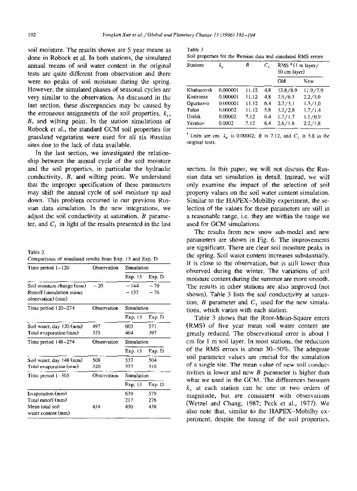
To understand the second problem, we show the simulations using the original snow sub-model for Ogurtsovo and Kostroma in Fig. 6a,b, and Fig. 6c,d, respectively. In these experiments, the model was integrated from 1978 for 6 years. The first year's results were discarded due to the influence of initial

Ogurtsovo (54.9N 83,0E) ~6

12 ° = = .

10

8

" N

FEB MAR APR MAY JUN JUL AUG SEP OCT NOV DEC Kostroma (57.8N 41.0E)

301 C

~" 24 . o

FEB MAR APR MAY JUN JUL AUG SEP OCT NOV DEC

16

12

10 t=

~ 4 .

2 .

N 0 -

Ogurtsovo (54.9N 83.0E)

b

F~B MJWR /~R WIAY ,ION JUL ALJG SEP OCT N(~V DEC Kostromo (57.8N 4.1.0E)

30-

27;

d 24-

c :

E

~ 9 ~ 6 ~ 3

m 0

d

FEB MAR APR MAY JUN JUL AUG SEP OCT NOV DEC

Fig. 6. Results of simulated soil moisture as compared to observations for (a) Ogurtsovo station in top 1 m; (b) Ogurtsovo station in top 0.5 m; (c) Kostroma station in top 1 m; (d) Kostroma station in top 0.5 m. Open circles: observations; open squares: new results; filled circles: old results.

192 Yong kan Xue et al. / Global and Planetary Change 13 (1996) 183-194

soil moisture. The results shown are 5 year means as done in Robock et al. In both stations, the simulated annual means of soil water content in the original tests are quite different from observation and there were no peaks of soil moisture during the spring. However, the simulated phases of seasonal cycles are very similar to the observation. As discussed in the last section, these discrepancies may be caused by the erroneous assignments of the soil properties, k s, B, and wilting point. In the station simulations of Robock et al., the standard GCM soil properties for grassland vegetation were used for all six Russian sites due to the lack of data available.

In the last section, we investigated the relationship between the annual cycle of the soil moisture and the soil properties, in particular the hydraulic conductivity, B, and wilting point. We understand that the improper specification of these parameters may shift the annual cycle of soil moisture up and down. This problem occurred in our previous Rus- sian data simulation. In the new integrations, we adjust the soil conductivity at saturation, B parameter, and C1 in light of the results presented in the last

Table 2 Comparisons of simulated results from Exp. 13 and Exp. D

Time period 1 - 120 Observation Simulation

Exp. 13 Exp. D

Soil moisture change (mm) - 20 - 144 - 79 Runoff (simulation minus - 137 - 76 observation) (ram)

Time period 120-274 Observation Simulation

Exp. 13 Exp. D

Soil water, day 120 (mm) 497 605 571 Total evaporation (mm) 375 464 397


Exp. 13 Exp. D

Soil water, day 148 (mm) 508 537 504 Total evaporation (mm) 320 377 310


Exp. t3 Exp. D

Evaporation (mm) 639 579 Total runoff (mm) 217 276 Mean total soil 434 430 438 water content (mm)

Table 3 Soil properties for the Russian data and simulated RMS errors

Stat ions k s B C l R M S a (1 m layer/ 50 cm layer)

Old New

Khabarovsk 0.000001 11.12 4.8 t3.8/8.9 11.9/7.9 Kostroma 0.000001 11.12 4.8 7.9/6.3 2.2/3.0 Ogurtsovo 0.000001 11.12 6.4 2.7/3.1 1.3/1.0 Tulun 0.00002 11.12 5.8 3.2/2.8 1.7/1.4 Uralsk 0.00002 7.12 6.4 1.7/ 1.7 1. t /0 .9 Yershov 0.0002 7.12 6.4 2.6/1.8 2.2/1.8

a Units are cm. k s is 0.00002; B is 7.12; and C 1 is 5.8 in the original tests.

section. In this paper, we will not discuss the Rus- sian data set simulation in detail. Instead, we will only examine the impact of the selection of soil property values on the soil water content simulation. Similar to the HAPEX-Mobi lhy experiment, the selection of the values for these parameters are still in a reasonable range, i.e. they are within the range we used for GCM simulations.

The results from new snow sub-model and new parameters are shown in Fig. 6. The improvements are significant. There are clear soil moisture peaks in the spring. Soil water content increases substantially. It is close to the observation, but is still lower than observed during the winter. The variations of soil moisture content during the summer are more smooth. The results in other stations are also improved (not shown). Table 3 lists the soil conductivity at saturation, B parameter and C 1 used for the new simulations, which varies with each station.

Table 3 shows that the Root-Mean-Square errors (RMS) of five year mean soil water content are greatly reduced. The observational error is about 1 cm for 1 m soil layer. In most stations, the reduction of the RMS errors is about 30-50%. The adequate soil parameter values are crucial for the simulation of a single site. The mean value of new soil conductivities is lower and new B parameter is higher than what we used in the GCM. The differences between k s at each station can be one or two orders of magnitude, but are consistent with observations (Wetzel and Chang, 1987; Peck et al., 1977). We also note that, similar to the HAPEX-Mobi lhy experiment, despite the tuning of the soil properties,

Yongkan Xue et a l . / Global and Planetary Change 13 (1996) 183-194 193

the model is still not able to precisely reproduce the observed soil moisture. The differences in Khabarovsk station are still quite large.

site to a larger scale, and to assess the impact of the lack of soil and vegetation property information on the model simulations.

5. Summary

In this paper, we have briefly reviewed SSiB's development and some of the major parameterizations in the model. The parameterizations for the soil sub-model are described more comprehensively since this is very much related to the sensitivity study described in this paper.

The sensitivity study shows that k s, B, and wilting point have a profound impact on the model simulation, but with different features. Both hydraulic conductivity at saturation and B parameter influence the soil moisture simulation by changing the soil hydraulic conductivity and the field capacity. The changes in equilibrium soil water content in this study are consistent with the changes in field capacity. However, the results in this study may be model dependent. For example, the effects of B parameter on the evaporation may be different for a model using different parameterization to calculate the bare soil evaporation.

The results of this study have revealed two causes of error in SSiB's test simulations (both the HAPEX and Russian simulations): the snowmelt partitioning parameterization and improper soil parameter specification. The springmelt problem of the Russian simulations is primarily due to the improper partitioning of snowmelt into infiltration and runoff. Moreover, from results presented in this paper, we find it is crucial to have adequate soil parameter values in the model to obtain realistic results in each station. The different Russian stations need to have different hydraulic conductivity values. The mean value of new soil conductivities is lower and new B parameter is greater than what we used in the GCM.

Since there are thousands of grid points in a GCM or a regional model, it is practically impossible to calibrate every grid point. In fact, using a single station as a representation for whole grid box is also questionable as we see from the Russian data experiment. Further study should be conducted to improve the soil model, to investigate the scaling problem, to develop an objective method of scaling from a single

Acknowledgements

The authors would like to thank Dr. A. Hender- son-Sellers for her leadership in this project and support to this study. We would also like thank Dr. P.J. Sellers for providing new snow codes. Special thanks for Dr. Peter Wetzel's very helpful discus- sions. This work was conducted under support from the National Science Foundation (NSF) through NSF grants EAR-94-05431, and the National Oceanic and Atmospheric Administration (NOAA) through NOAA grant NA46GP0340-02.

References

Blackman, P.G. and Davies, W.J., 1985. Root to shoot communi- cation in maize plants of the effects of soil drying. J. Exp. Bot., 36: 39-48.

Brooks, R.H. and Corey, A.T., 1964. Hydraulic properties of porous media. Colo. State Univ. Hydrol. Pap., 3.

Camillo, P.J. and Gumey, R.J., 1986. A resistance parameter for bare-soil evaporation models. Soil Sci., 2: 95-105.

Chen, T.H. et al., 1995. Cabauw experimental results from the project for intercomparison of land surface parameterization schemes. J. Climate, submitted.

Chen, F., Mitchell, K., Schaake, J., Xue, Y., Pan, H.-L., Koren, V., Duan, Q. and Betts, A., 1995a. Modeling of land-surface evaporation by four schemes and comparison with FIFE observations. J. Geophys. Res., 101(D3): 7251-7268.

Clapp, R.B. and Homberger, G.M., 1978. Empirical equations for some soil hydraulic properties. Water Resour. Res., 14: 601- 604.

Cosby, B.J., Homberger, G.M., Clapp, R.B. and Girm, T.R., 1984. A statistical exploration of the relationship of soil moisture characteristics to the physical properties of soils. Water Re- sour. Res., 20: 682-690.

Ek, M. and Cuenca, R.H., 1994. Variation in soil parameters: Implications for modeling surface fluxes and atmospheric boundary-layer development. Boundary-Layer Meteorol., 70: 369-383.

Federer, C.A., 1979. A soil-plant-atmosphere model for transpiration and availability of soil water. Water Resour. Res., 153: 555-562.

Fennessy, M.J. and Xue, Y., 1994. Impact of vegetation map on GCM seasonal simulations over the United States. Ecol. Ap- plic., in press.

Gardner, W.R., 1958. Some steady-state solutions of the unsatu-

194 Yongkan Xue et a l . / Global and Planetary Change 13 (1996) 183-194

rated moisture flow equation with application to evaporation from a water table. Soil Sci., 85: 228-232.

Hillel, D., 1982. Introduction to Soil Physics. Academic Press, New York, 364 pp.

Jarvis, P.G., 1976. The interpretation of the variations in leaf water potential and stomatal conductance found in canopies in the field. Philos. Trans. R. Soc. London, Ser. B., 273: 593-610.

Liston, G.E., Sud, Y.C. and Wood, E.F., 1994. Evaluating GCM land surface hydrology parameterizations by computing river discharges using a runoff routing model: application to the Mississippi basin. J. Appl. Meteorol., 33: 394-405.

Mahfouf, J.-F., Ciret, C., Duchame, A., lrannejad, P., Noilhan, J., Shao, Y., Thornton, P., Xue, Y. and Yang, Z.-L., 1996. Analysis of transpiration results from the RICE and PILPS Workshop. Global Planet. Change, 13: 73-88.

Peck, A.J., Luxmore, R.J. and Stolzy, J.L., 1977. Effects of spatial variability of soil hydraulic properties in water budget modeling. Water Resour. Res., 13: 348-354.

Robock, A., Vinnikov, K.V., Schlosser, V.A., Speranskaya, N.A. and Xue, Y., 1995. Use of Russian soil moisture and meteoro- logical observations to validate soil moisture simulations with biosphere and bucket models. J. Climate, 8: 15-35.

Sato, N., Sellers, P.J., Randall, D.A., Schneider, E.K., Shukla, J., Kinter, J.L., III, Hou, Y.-T. and Albertazzi, E., 1989. Effects of implementing the simple biosphere model in a general circulation model. J. Atmos. Sci., 46: 2757-2782.

Shao, Y. and A. Henderson-Sellers, 1996. Soil moisture simulation workshop review. Global Planet. Change, 12: 54-90.

Schlosser, C.A., 1995. Land-surface hydrology: validation and intercomparison of multi-year off-line simulations using mid- latitude data. Thesis. Univ. Maryland, College Park, 132 pp.

Sellers, P.J., Mintz, Y., Sud, Y.C. and Dalcher, A., 1986. A simple biosphere model (SIB) for use within general circulation models. J. Atmos. Sci., 43: 505-531.

Sellers, P.J., Randall, D.A., Collatz, C.J., Berry, J.A., Field, C.B., Dazlich, D.A., Zhang, C. and Collelo, G.D., 1995. A revised land surface parameterization (SiB2) for atmospheric GCMs. Part 1: model formulation. J. Climate, in press.

Van Genuchten, M.T., 1980. A close-form equation for predicting the hydraulic conductivity of unsaturated soils. Soil Sci. Soc. Am. J., 44: 892-898.

Wetzel, P. and Chang, J.-T., 1987. Concerning the relationship between evapotranspiration and soil moisture. J. Climate Appl. Meteorol., 26: 18-27.

Xue, Y., 1995. The impact of desertification in the Mongolian and the Inner Mongolian grassland on the East Asian Monsoon. J. Climate, in press.

Xue, Y. and Allen, S., 1995. Testing a biosphere model (SSiB for the Sahelian Semi-Arid area using field data. In: AMS Conf. Hydrology, 1995, pp. 93-98 (preprin0.

Xue, Y. and Sbukla, J., 1993a. The influence of land surface properties on Sahel climate. Part I: desertification. J. Climate, 6: 2232-2245.

Xue, Y. and Shukla, J., 1993b. The influence of land surface properties on Sahel climate. Part II: Afforestation. J. Climate, in press.

Xue, Y., Sellers, P.J., Kinter, J.L., III and Shukla, J., 1991. A simplified biosphere model for global climate studies. J. Cli- mate, 4: 345-364.

Xue, Y., Bastable, N., Dirmeyer, P.J. and Sellers, P.J., 1996a. Sensitivity of simulated surface fluxes to changes in land surface parameterization--a study using ABRACOS data. J. Appl. Meteorol., 35: 386-400.

Xue, Y., Fennessy, M.J. and Sellers, P.J., 1996b. Impact of vegetation properties on U.S. summer weather prediction. J. Geophys. Res., 101(D3): 7419-7430.

ssib and its sensitivity to soil properties a case study

Documents