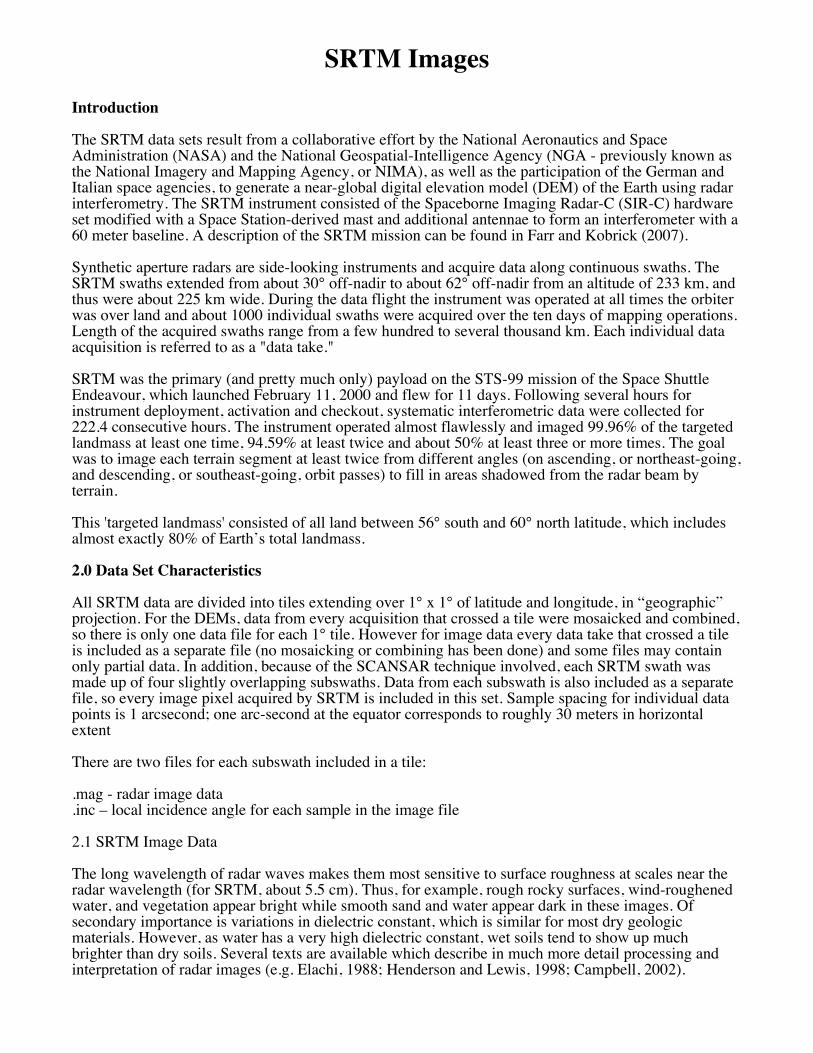
srtm images - usgs€¦ · srtm images introduction the srtm data sets result from a collaborative...
TRANSCRIPT
SRTM Images Introduction The SRTM data sets result from a collaborative effort by the National Aeronautics and Space Administration (NASA) and the National Geospatial-Intelligence Agency (NGA - previously known as the National Imagery and Mapping Agency, or NIMA), as well as the participation of the German and Italian space agencies, to generate a near-global digital elevation model (DEM) of the Earth using radar interferometry. The SRTM instrument consisted of the Spaceborne Imaging Radar-C (SIR-C) hardware set modified with a Space Station-derived mast and additional antennae to form an interferometer with a 60 meter baseline. A description of the SRTM mission can be found in Farr and Kobrick (2007). Synthetic aperture radars are side-looking instruments and acquire data along continuous swaths. The SRTM swaths extended from about 30° off-nadir to about 62° off-nadir from an altitude of 233 km, and thus were about 225 km wide. During the data flight the instrument was operated at all times the orbiter was over land and about 1000 individual swaths were acquired over the ten days of mapping operations. Length of the acquired swaths range from a few hundred to several thousand km. Each individual data acquisition is referred to as a "data take." SRTM was the primary (and pretty much only) payload on the STS-99 mission of the Space Shuttle Endeavour, which launched February 11, 2000 and flew for 11 days. Following several hours for instrument deployment, activation and checkout, systematic interferometric data were collected for 222.4 consecutive hours. The instrument operated almost flawlessly and imaged 99.96% of the targeted landmass at least one time, 94.59% at least twice and about 50% at least three or more times. The goal was to image each terrain segment at least twice from different angles (on ascending, or northeast-going, and descending, or southeast-going, orbit passes) to fill in areas shadowed from the radar beam by terrain. This 'targeted landmass' consisted of all land between 56° south and 60° north latitude, which includes almost exactly 80% of Earth’s total landmass. 2.0 Data Set Characteristics All SRTM data are divided into tiles extending over 1° x 1° of latitude and longitude, in “geographic” projection. For the DEMs, data from every acquisition that crossed a tile were mosaicked and combined, so there is only one data file for each 1° tile. However for image data every data take that crossed a tile is included as a separate file (no mosaicking or combining has been done) and some files may contain only partial data. In addition, because of the SCANSAR technique involved, each SRTM swath was made up of four slightly overlapping subswaths. Data from each subswath is also included as a separate file, so every image pixel acquired by SRTM is included in this set. Sample spacing for individual data points is 1 arcsecond; one arc-second at the equator corresponds to roughly 30 meters in horizontal extent There are two files for each subswath included in a tile: .mag - radar image data .inc – local incidence angle for each sample in the image file 2.1 SRTM Image Data The long wavelength of radar waves makes them most sensitive to surface roughness at scales near the radar wavelength (for SRTM, about 5.5 cm). Thus, for example, rough rocky surfaces, wind-roughened water, and vegetation appear bright while smooth sand and water appear dark in these images. Of secondary importance is variations in dielectric constant, which is similar for most dry geologic materials. However, as water has a very high dielectric constant, wet soils tend to show up much brighter than dry soils. Several texts are available which describe in much more detail processing and interpretation of radar images (e.g. Elachi, 1988; Henderson and Lewis, 1998; Campbell, 2002).

As radar images are acquired in a side-looking geometry, they can be distorted by topographic variations. Because SRTM acquired topography at the same time as the image data and the two are inherently registered, it was an easy matter to orthorectify the image data. This also means that voids present in the SRTM DEM produce voids in the image data. The SRTM radar image product provides the mean surface backscatter coefficients of the mapped areas. This required the image processor to be radiometrically calibrated. For SRTM, the goals for absolute and relative radiometric calibration were 3 dB and 1 dB respectively. The SRTM main antenna was the major source of calibration error as it was a large active array antenna. In the spaceborne environment, both zero gravity unloading and the large variation in temperature caused distortions in the phased array. Hundreds of phase shifters and transmit / receive modules populated the C-band antenna panels. Monitoring the performance of each module was very difficult, causing inaccuracies in the antenna pattern predictions, in particular in elevation, as the beams were spoiled to obtain a wide swath. Therefore antenna elevation pattern correction coefficients were derived with empirical methods using data takes over the Amazon rain forest. As the Amazon rainforest is an homogeneous and isotropic area, the backscatter coefficient is almost independent of the look angle. Without compensation, a scalloping effect would have been visible in the sub-swath and full-swath images. Speckle noise is present in the image data. This is a characteristic of coherent imaging systems and appears as a random, high-frequency, salt and pepper effect. Most imaging radar systems average many ‘looks’, however SRTM was optimized for a wide swath and thus acquired only 1-2 looks per sub-swath causing a relatively high speckle noise level. 2.2 SRTM Incidence Angle Data Because local incidence angle is so important for interpretation of radar images, a file containing that information is provided for each of the image files. The values are calculated from the position of the Shuttle and the DEM. They represent the angle between the radar beam and the local normal to the surface at each pixel. Because this information could be used to ‘back-calculate’ a DEM, the incidence angle pixels were averaged 3x3 and sampled back to 1 arc-second in order to remain registered with the corresponding image file. The figure below shows a portion of cell N34W119, demonstrating the characteristics of the image and incidence angle data sets and the difference with the topographic data.
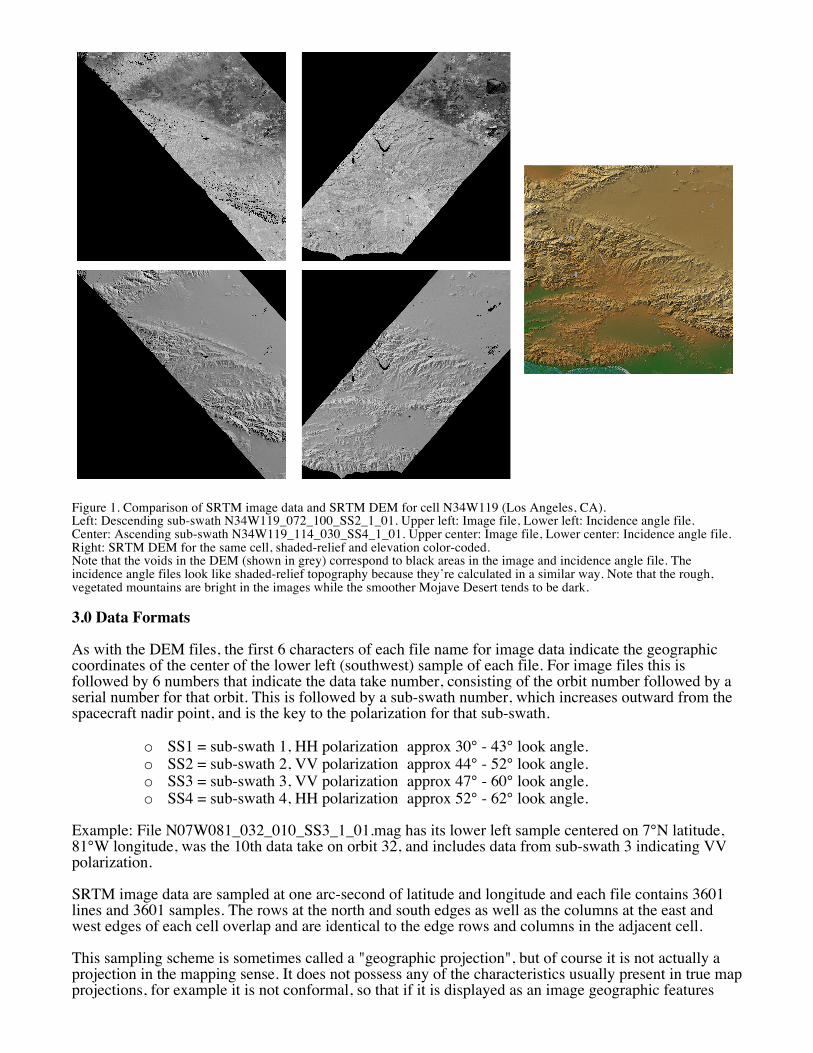
Figure 1. Comparison of SRTM image data and SRTM DEM for cell N34W119 (Los Angeles, CA). Left: Descending sub-swath N34W119_072_100_SS2_1_01. Upper left: Image file, Lower left: Incidence angle file. Center: Ascending sub-swath N34W119_114_030_SS4_1_01. Upper center: Image file, Lower center: Incidence angle file. Right: SRTM DEM for the same cell, shaded-relief and elevation color-coded. Note that the voids in the DEM (shown in grey) correspond to black areas in the image and incidence angle file. The incidence angle files look like shaded-relief topography because they’re calculated in a similar way. Note that the rough, vegetated mountains are bright in the images while the smoother Mojave Desert tends to be dark. 3.0 Data Formats As with the DEM files, the first 6 characters of each file name for image data indicate the geographic coordinates of the center of the lower left (southwest) sample of each file. For image files this is followed by 6 numbers that indicate the data take number, consisting of the orbit number followed by a serial number for that orbit. This is followed by a sub-swath number, which increases outward from the spacecraft nadir point, and is the key to the polarization for that sub-swath.
o SS1 = sub-swath 1, HH polarization approx 30° - 43° look angle. o SS2 = sub-swath 2, VV polarization approx 44° - 52° look angle. o SS3 = sub-swath 3, VV polarization approx 47° - 60° look angle. o SS4 = sub-swath 4, HH polarization approx 52° - 62° look angle.
Example: File N07W081_032_010_SS3_1_01.mag has its lower left sample centered on 7°N latitude, 81°W longitude, was the 10th data take on orbit 32, and includes data from sub-swath 3 indicating VV polarization. SRTM image data are sampled at one arc-second of latitude and longitude and each file contains 3601 lines and 3601 samples. The rows at the north and south edges as well as the columns at the east and west edges of each cell overlap and are identical to the edge rows and columns in the adjacent cell. This sampling scheme is sometimes called a "geographic projection", but of course it is not actually a projection in the mapping sense. It does not possess any of the characteristics usually present in true map projections, for example it is not conformal, so that if it is displayed as an image geographic features

will be distorted. However it is quite easy to handle mathematically, can be easily imported into most image processing and GIS software packages, and multiple cells can be assembled easily into a larger mosaic (unlike the pesky UTM projection, for example.) 3.1 Image File (.mag) Image brightness or magnitude is given as 8 bits/sample, with the values indicating radar cross section, scaled linearly between -50 dB and +40 dB. Data numbers (DN) can be converted to backscatter cross section in dB using the expression dB = 0.3529*DN - 50. There are no header or trailer bytes embedded in the file. The data are stored in row major order (all the data for row 1, followed by all the data for row 2, etc.). These data also contain occasional voids from a number of causes such as shadowing, phase unwrapping anomalies, or other radar-specific causes. Voids have the value 0. 3.2 Incidence Angle File (.inc) Local incidence angle is provided as 16-bit integer data in a simple binary raster. There are no header or trailer bytes embedded in the file. The data are stored in row major order (all the data for row 1, followed by all the data for row 2, etc.). The pixel values represent hundredths of a degree (i.e. 4321 = 43.21°). Byte order is Motorola ("big-endian") standard with the most significant byte first. Because the incidence angle data are stored in a 2-byte binary format, users must be aware of how the bytes are addressed on their computers. The incidence angle data are provided in Motorola or IEEE byte order, which stores the most significant byte first ("big endian"). Systems such as Sun SPARC and Silicon Graphics workstations and Macintosh computers use the Motorola byte order. The Intel byte order, which stores the least significant byte first ("little endian"), is used on DEC Alpha systems and most PCs. Users with systems that address bytes in the Intel byte order may have to "swap bytes" of the incidence angle data unless their application software performs the conversion during ingest. These data also contain occasional voids from a number of causes such as shadowing, phase unwrapping anomalies, or other radar-specific causes. Voids have the value 0. 4.0 References Campbell, B.A., 2002, Radar Remote Sensing of Planetary Surfaces, Cambridge Univ. Press, Cambridge, UK, 331 pp. Elachi, C., 1988, Spaceborne Radar Remote Sensing: Applications and Techniques, IEEE Press, New York, 254 pp. Farr, T.G., E. Caro, R. Crippen, R. Duren, S. Hensley, M. Kobrick, M. Paller, E. Rodriguez, P. Rosen, L. Roth, D. Seal, S. Shaffer, J. Shimada, J. Umland, M. Werner, M. Oskin, D. Burbank, D. Alsdorf, 2007, The Shuttle Radar Topography Mission, v. 45, Reviews of Geophysics, doi: 1029/2005RG000183. Henderson, F.M., A.J. Lewis, ed., 1998, Principles and Applications of Imaging Radar, Manual of Remote Sensing, v. 2, Wiley, NY, 866 pp. Web sites of interest: NASA/JPL SRTM: http://www.jpl.nasa.gov/srtm/ Data access: http://www2.jpl.nasa.gov/srtm/cbanddataproducts.html US Geological Survey: http://srtm.usgs.gov/