srm_lecture_6_2012.pdf

1

©A. Alizadeh Shipping Risk Management Slide 1

Shipping Risk Management

Credit Risk Measurement & Management


What is Credit Risk?!

• Atlas Shipping files for bankruptcy– Lloyds List, Craig Eason - Thursday 18 December 2008

– DANISH dry bulk operator, Atlas Shipping has filed for bankruptcy. Following a petition to the Danish

Maritime and Commercial Court the company issued a statement today saying that with the current tight

market it will run out of cash in three months with a liquidity loss of $3m a week.

• Armada Singapore seeks to restructure in face of charterer defaults – Lloyds List, By Marcus Hand in Singapore - Tuesday 6 January 2009

– MAJOR dry bulk shipping operator Armada (Singapore) is seeking protection from creditors while it

restructures in the face of hundreds of millions of dollars worth of charterer defaults.

• Bankruptcies set ‘to increase’ despite dry bulk rates recovery– Lloyds List, Thursday 19 February 2009

– Deloitte’s head of shipping also forecasts refinancing difficulties

– THIS month’s surge in the Baltic Dry Index may indicate “a path to recovery” for the dry freight market,

but further shipowner bankruptcies are likely, according to consultancy Deloitte.

2


What is Credit Risk?!

• Samsun seeks bankruptcy protection in US– Lloyds List, Rajesh Joshi and Keith Wallis - Thursday 12 March 2009

– SAMSUN Logix has become the fourth shipping company to seek parallel bankruptcy protection in

New York, after being granted similar protection by Seoul’s central district court.

• US Shipping goes bankrupt– Lloyds List, Rajesh Joshi, New York - Thursday 30 April 2009

– US SHIPPING Partners has thrown in the towel one year after first revealing its troubles with lenders,

applying to the US Bankruptcy Court for Chapter 11 protection. Paul Gridley and Albert Bergeron, who

departed last year as US Shipping’s chief executive and chief financial officer respectively, have now

surfaced as creditors, to whom US Shipping owes close to $1m each. The New York-listed Jones Act

tanker company, which is a limited partnership, had a deadline of April 30 to hammer out an acceptable

restructuring with its lenders. The Chapter 11 petition was filed a day earlier, instead of seeking another

loan extension.

• Nexus seeks extra time to repay interest

– Lloyds List, Martyn Wingrove - Tuesday 9 June 2009

– NORWEGIAN ship owner Nexus Floating Production has called on its bondholders to plead for more

time for interest repayments. Nexus’ failure to gain a long-term lease contract for its first oil production

ship means it would be unable to pay bond holders this month.


Topics Covered• What is Credit Risk

• Probability of default

• Loss given default

• Sources of Credit Risk in Shipping

• Qualitative & Quantitative Approaches in Credit Risk Analysis

• Credit Ratings and Credit Rating Agencies

• Extracting Default Probabilities & Recovery Rates

• Credit Derivatives

• CDS, TRS, CDO

• CreditMetrics

Credit Risk Measurement & Management

3


Credit Risk in Shipping

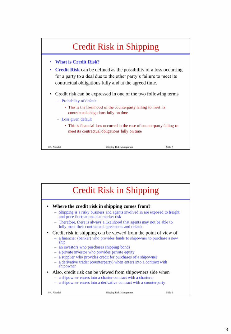
• What is Credit Risk?

• Credit Risk can be defined as the possibility of a loss occurring

for a party to a deal due to the other party’s failure to meet its

contractual obligations fully and at the agreed time.

• Credit risk can be expressed in one of the two following terms

– Probability of default

• This is the likelihood of the counterparty failing to meet its

contractual obligations fully on time

– Loss given default

• This is financial loss occurred in the case of counterparty failing to

meet its contractual obligations fully on time



• Where the credit risk in shipping comes from?

– Shipping is a risky business and agents involved in are exposed to freight and price fluctuations due market risk

– Therefore, there is always a likelihood that agents may not be able to fully meet their contractual agreements and default

• Credit risk in shipping can be viewed from the point of view of – a financier (banker) who provides funds to shipowner to purchase a new

ship

– an investors who purchases shipping bonds

– a private investor who provides private equity

– a supplier who provides credit for purchases of a shipowner

– a derivative trader (counterparty) when enters into a contract with shipowner

• Also, credit risk can be viewed from shipowners side when– a shipowner enters into a charter contract with a charterer

– a shipowner enters into a derivative contract with a counterparty

4



• Qualitative Credit Risk

analysis uses firm specific

factors which are not

quantifiable such as

– Reputation/Business History

– Managerial expertise and track

record

– Relative standing in the market

– Financial flexibility and capital

structure

– Strength and operating flexibility

– Strategic plans and contingencies

Qualitative vs Quantitative Credit Risk Analysis

• Quantitative Credit Risk analysis

uses industry and

macroeconomic factors which

are quantifiable such as

– Financial heath of the firm

– Firm size

– Earnings (interest coverage)

– Gearing (debt to equity ratio)

– Turnover and ROC

– Market conditions

– Interest rates

– Cashflow Uncertainty



• The Credit Risk measurement is been traditionally used in the

bond market mainly in classifying and pricing corporate bonds

• Corporate bond are classified by certain agencies (Moodys,

S&P, Fitch, and others) according to the capability of issuers in

repaying their debt

– Credit Rating is meant to be an indication of the likelihood that a

company will repay its debt on time, i.e. a measure of credit risk.

– Credit Ratings are therefore, opinions of future relative creditworthiness

and provide objective, consistent and simple measures to indicate the

likelihood that a company will repay its debt on time

• In what follows we focus on quantitative approaches in

measuring Credit Risk

5



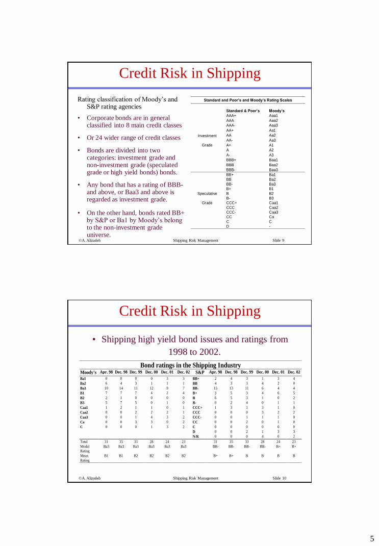
Rating classification of Moody’s and S&P rating agencies

• Corporate bonds are in general classified into 8 main credit classes

• Or 24 wider range of credit classes

• Bonds are divided into two categories: investment grade and non-investment grade (speculated grade or high yield bonds) bonds.

• Any bond that has a rating of BBB-and above, or Baa3 and above is regarded as investment grade.

• On the other hand, bonds rated BB+ by S&P or Ba1 by Moody’s belong to the non-investment grade universe.

Standard and Poor’s and Moody’s Rating Scales

Standard & Poor’s Moody’s

AAA+ Aaa1

AAA Aaa2

AAA- Aaa3

AA+ Aa1

AA Aa2

AA- Aa3

A+ A1

A A2

A- A3

BBB+ Baa1

BBB Baa2

Investment

Grade

BBB- Baa3

BB+ Ba1

BB Ba2BB- Ba3B+ B1

B B2B- B3CCC+ Caa1

CCC Caa2CCC- Caa3CC Ca

C C

Speculative

Grade

D -



• Shipping high yield bond issues and ratings from

1998 to 2002.

Bond ratings in the Shipping IndustryMoody's Apr. 98 Dec. 98 Dec. 99 Dec. 00 Dec. 01 Dec. 02 S&P Apr. 98 Dec. 98 Dec. 99 Dec. 00 Dec. 01 Dec. 02

Ba1 0 0 0 0 3 3 BB+ 2 4 3 1 3 4

Ba2 6 4 3 1 1 1 BB 4 3 3 4 2 0

Ba3 10 14 11 12 9 7 BB- 15 13 11 6 4 4

B1 7 7 7 4 2 4 B+ 3 5 3 4 6 5

B2 2 1 0 0 0 0 B 6 5 3 1 0 2

B3 5 7 5 0 1 0 B- 0 2 4 0 1 1

Caa1 1 2 1 1 0 1 CCC+ 1 3 1 3 1 0

Caa2 0 0 2 2 2 1 CCC 0 0 0 3 2 2

Caa3 0 0 1 4 3 2 CCC- 0 0 1 1 1 0

Ca 0 0 3 3 0 2 CC 0 0 2 0 1 0

C 0 0 0 1 3 2 C 0 0 0 0 0 0

D 0 0 2 1 3 3

N/R 0 0 0 4 0 2

Total 31 35 33 28 24 23 31 35 33 28 24 23

Modal

Rating

Ba3 Ba3 Ba3 Ba3 Ba3 Ba3 BB- BB- BB- BB- B+ B+

Mean

Rating

B1 B1 B2 B2 B2 B2 B+ B+ B B B B

6



• Yield is defined as the percentage rate of return on the bond.

• The yield premium is defined as the difference between the yield to maturity on a corporate bond and the yield to maturity on a government bond of the same maturity (risk free rate).

• Traders regularly estimate yield curves for bonds with different credit ratings. – Yield premium can be used estimate probabilities of default.

• The excess of the value of a risk-free bond over a similar corporate bond equals the present value of the cost of defaults.



Plot of average yield premium on shipping high yield bonds

with different rating over the period 1998 to 2002

Figure 1:Yield Premium vs Rating

Shipping High Yield Bonds, April 1998 - December 2002

0

500

1000

1500

2000

2500

3000

3500

4000

Rating (BB+=11…C=1)

Yie

ld P

rem

ium

(b

asis

poin

ts)

3727 2386 2500 1677 1084 1023 654 450 329

CC CCC- CCC+ B- B B+ BB- BB BB+

7



However, yield premium changes over time due to variety of reasons including market conditions

0

2

4

6

8

10

12

14

Jan

-94

Jan

-95

Jan

-96

Jan

-97

Jan

-98

Jan

-99

Jan

-00

Jan

-01

Jan

-02

Jan

-03

Jan

-04

Jan

-05

Jan

-06

Jan

-07

Jan

-08

Yie

ld P

rem

ium

in

%

LB_BB LB_B ML_SHIP


Typical Pattern of Yield Curves

Spread

over

Treasuries

Maturity

Baa/BBB

A/A

Aa/AA

Aaa/AAA

Sample yield spread curves for bonds with different ratings

8


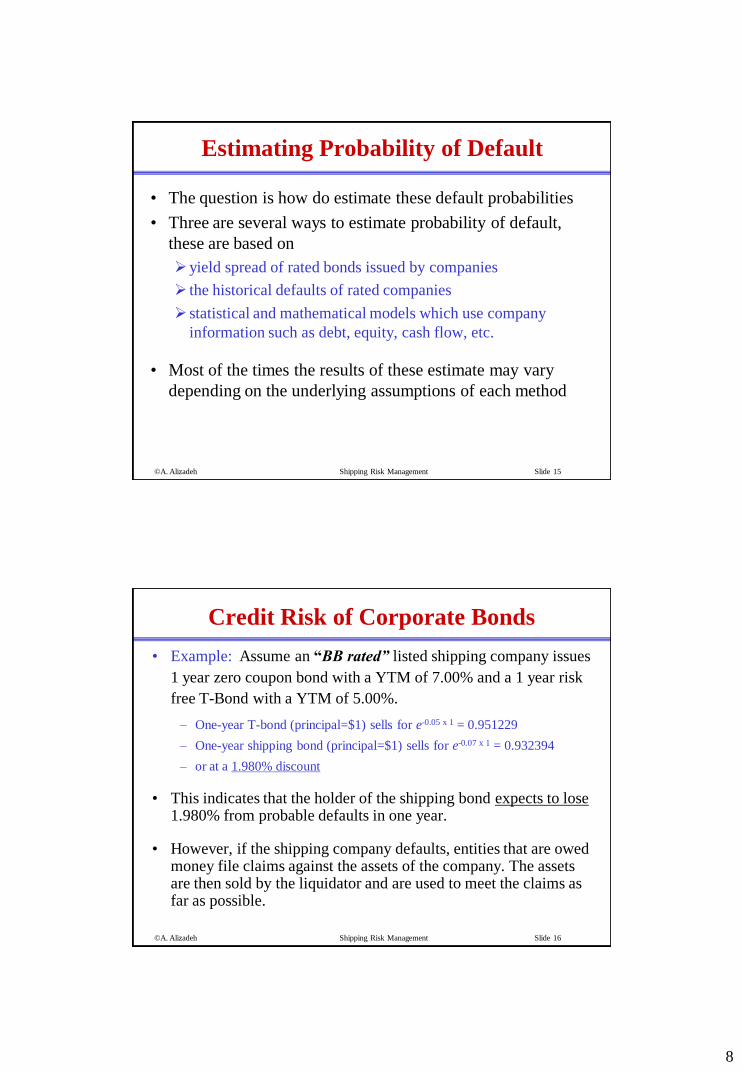
Estimating Probability of Default

• The question is how do estimate these default probabilities

• Three are several ways to estimate probability of default,

these are based on

yield spread of rated bonds issued by companies

the historical defaults of rated companies

statistical and mathematical models which use company

information such as debt, equity, cash flow, etc.

• Most of the times the results of these estimate may vary

depending on the underlying assumptions of each method


Credit Risk of Corporate Bonds

• Example: Assume an “BB rated” listed shipping company issues

1 year zero coupon bond with a YTM of 7.00% and a 1 year risk

free T-Bond with a YTM of 5.00%.

– One-year T-bond (principal=$1) sells for e-0.05 x 1 = 0.951229

– One-year shipping bond (principal=$1) sells for e-0.07 x 1 = 0.932394

– or at a 1.980% discount

• This indicates that the holder of the shipping bond expects to lose1.980% from probable defaults in one year.

• However, if the shipping company defaults, entities that are owed money file claims against the assets of the company. The assets are then sold by the liquidator and are used to meet the claims as far as possible.

9


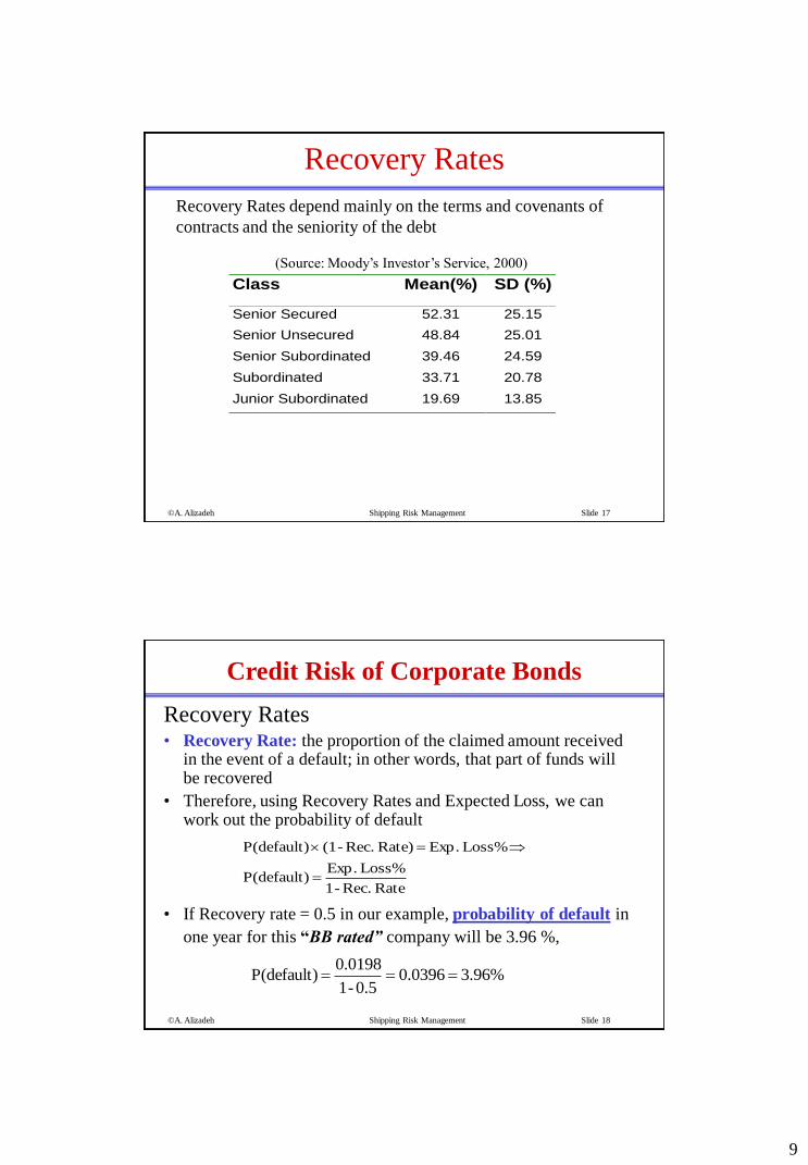
Recovery Rates

Class Mean(%) SD (%)

Senior Secured 52.31 25.15

Senior Unsecured 48.84 25.01

Senior Subordinated 39.46 24.59

Subordinated 33.71 20.78

Junior Subordinated 19.69 13.85

Recovery Rates depend mainly on the terms and covenants of

contracts and the seniority of the debt

(Source: Moody’s Investor’s Service, 2000)


Recovery Rates• Recovery Rate: the proportion of the claimed amount received

in the event of a default; in other words, that part of funds will be recovered

• Therefore, using Recovery Rates and Expected Loss, we can work out the probability of default

• If Recovery rate = 0.5 in our example, probability of default in

one year for this “BB rated” company will be 3.96 %,

Rate Rec.-1

Loss% Exp.P(default)

Loss% Exp. Rate) Rec.-(1 P(default)

%96.30396.00.5-1

0.0198P(default)

Credit Risk of Corporate Bonds

10


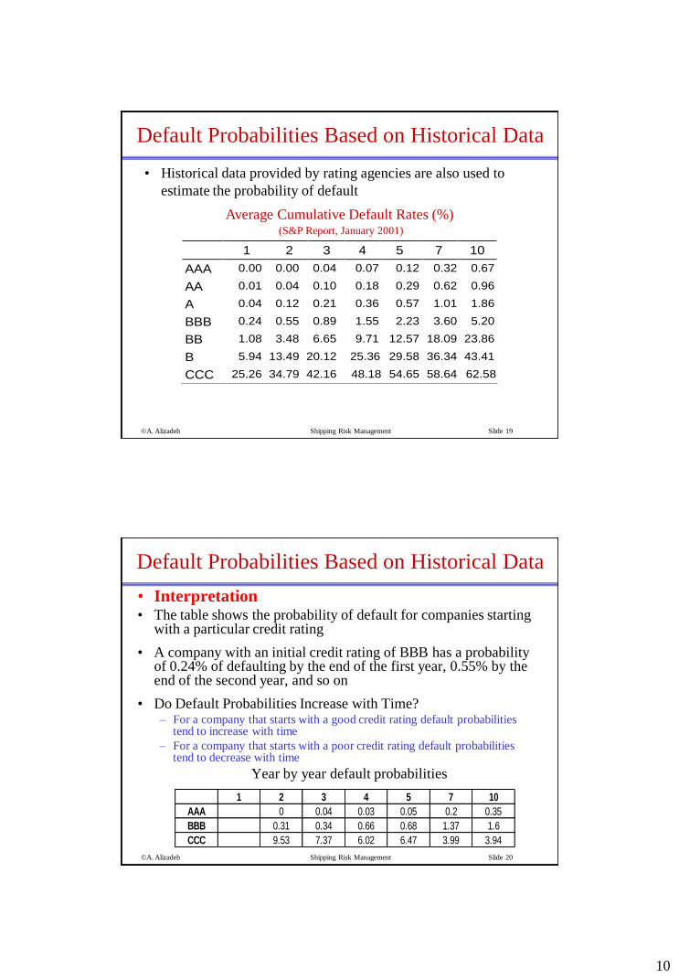
Default Probabilities Based on Historical Data

• Historical data provided by rating agencies are also used to

estimate the probability of default

Average Cumulative Default Rates (%)(S&P Report, January 2001)

1 2 3 4 5 7 10

AAA 0.00 0.00 0.04 0.07 0.12 0.32 0.67

AA 0.01 0.04 0.10 0.18 0.29 0.62 0.96

A 0.04 0.12 0.21 0.36 0.57 1.01 1.86

BBB 0.24 0.55 0.89 1.55 2.23 3.60 5.20

BB 1.08 3.48 6.65 9.71 12.57 18.09 23.86

B 5.94 13.49 20.12 25.36 29.58 36.34 43.41

CCC 25.26 34.79 42.16 48.18 54.65 58.64 62.58


• Interpretation• The table shows the probability of default for companies starting

with a particular credit rating

• A company with an initial credit rating of BBB has a probability of 0.24% of defaulting by the end of the first year, 0.55% by the end of the second year, and so on

• Do Default Probabilities Increase with Time?– For a company that starts with a good credit rating default probabilities

tend to increase with time

– For a company that starts with a poor credit rating default probabilities tend to decrease with time

Year by year default probabilities

1 2 3 4 5 7 10

AAA 0 0.04 0.03 0.05 0.2 0.35

BBB 0.31 0.34 0.66 0.68 1.37 1.6

CCC 9.53 7.37 6.02 6.47 3.99 3.94

Default Probabilities Based on Historical Data

11


Bond Prices vs Historical Default Experience

• The estimates of the probability of default calculated from bond

prices are much higher than those from historical data.

• Consider for example BB-rated bonds. These typically yield at

least 650 bps more than Treasuries

– This means that we expect to lose at least 1 - e-0.065 x 5 = 0.2774 or 27.74%

of the bonds value over a 5-year period. Assuming a low recovery rate of

30%, the probability of default is then 27.74/0.7 = 55.49%.

– This is over 4 times greater than the 12.57% historical probability

• Possible reasons for these results

– The liquidity of corporate bonds is less than that of Treasury bonds

– Bonds traders may be factoring into their pricing depression scenarios

much worse than anything seen in the last 20 years


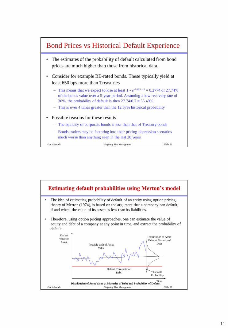
Estimating default probabilities using Merton’s model

• The idea of estimating probability of default of an entity using option pricing

theory of Merton (1974), is based on the argument that a company can default,

if and when, the value of its assets is less than its liabilities.

• Therefore, using option pricing approaches, one can estimate the value of

equity and debt of a company at any point in time, and extract the probability of

default.

Market

Value of

AssetPossible path of Asset

Value

Default Threshold or

Debt

Time

Default

Probability

Distribution of Asset

Value at Maturity of

Debt

Distribution of Asset Value at Maturity of Debt and Probability of Default

12



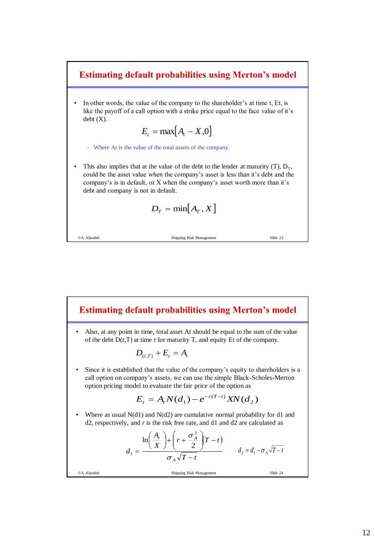
• In other words, the value of the company to the shareholder’s at time t, Et, is

like the payoff of a call option with a strike price equal to the face value of it’s

debt (X).

– Where At is the value of the total assets of the company.

• This also implies that at the value of the debt to the lender at maturity (T), DT,

could be the asset value when the company’s asset is less than it’s debt and the

company’s is in default, or X when the company’s asset worth more than it’s

debt and company is not in default.

0,max XAE tt

XAD TT ,min


• Also, at any point in time, total asset At should be equal to the sum of the value

of the debt D(t,T) at time t for maturity T, and equity Et of the company.

• Since it is established that the value of the company’s equity to shareholders is a

call option on company’s assets, we can use the simple Black-Scholes-Merton

option pricing model to evaluate the fair price of the option as

• Where as usual N(d1) and N(d2) are cumulative normal probability for d1 and

d2, respectively, and r is the risk free rate, and d1 and d2 are calculated as


ttTt AED ),(

)()( 2

)(

1 dXNedNAE tTr

tt

tT

tTrX

A

dA

At

2ln

2

1tTdd A 12

13


• Once the value of equity at time t, Et, is estimated using the pricing formula, it

can be deducted from the asset value of the firm at time t At to obtain the debt

value.

• It can be noted that the N(d2) is the risk neutral probability that at maturity of

the debt the company’s asset value be greater than the debt, and the company

does not default. Whereas, 1-N(d2), is the risk neutral probability that at

maturity of the debt, the company’s asset value be less than it’s debt, and the

company defaults.

• Furthermore, having obtained the value of debt at time t for maturity T, D(t,T),

we can calculate the yield y(t,T) debt.


ttTt EAD ),(

tT

DXy

Tt

Tt

)ln()ln( ),(

),(


• Example: consider a one vessel shipping company with current asset value of

$120m out of which $100m is debt with 1 year to maturity. The volatility of the

vessel’s price is 30%, while the current one year risk free rate is 5%. Based on

the information, we can estimate the current value of the company’s equity,

current value of debt, the yield on the debt, and the probability of default.

• Using the Black-Scholes-Merton model, we first calculate d1, d2, and

corresponding cumulative probabilities.


8224.0)N(d 9244.013.0

12

3.005.0

100

120ln

1

2

1

d

7338.0)N(d 6244.0)1(3.09244.0 212 tTdd A

14


• Using the above probabilities and the option pricing formula in equation (5),

current equity value and debt can be calculated as

• Moreover, the yield and the credit premium for this debt can be calculated using

equation (7) as 9.3% and 4.3%, respectively, and the default probability based on

[1-N(d2)] will be 26.62%.

• In addition, the present value of no default debt is $95.123m, which means that

expected loss on this debt is 4.21% [(95.123-91.12)/95.123], therefore, we can

estimate the expected recovery in the event of default of the debt as

28.88m$

)7338.0)(100()8224.0(120)()( )1*05.0(

2

)(

1

edXNedNAE tTr

tt

mmmEAD ttTt 12.91$88.28$120$),(


%19.842662.0

0421.01

P(default)

Loss% Exp.1Recovery Expected


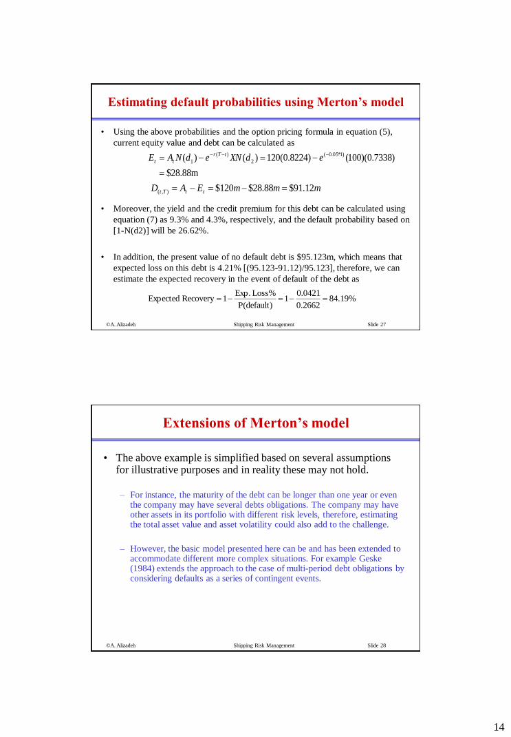
• The above example is simplified based on several assumptions for illustrative purposes and in reality these may not hold.

– For instance, the maturity of the debt can be longer than one year or even the company may have several debts obligations. The company may have other assets in its portfolio with different risk levels, therefore, estimating the total asset value and asset volatility could also add to the challenge.

– However, the basic model presented here can be and has been extended to accommodate different more complex situations. For example Geske (1984) extends the approach to the case of multi-period debt obligations by considering defaults as a series of contingent events.

Extensions of Merton’s model

15


Credit Risk Management

Credit Derivatives


Reducing Credit Exposure• Collateralization

– Where the lender takes some form of collateral for security (securitisation).

– The lender may ask for guarantees (letter of credit)

• Downgrade triggers– Where the lender sets thresholds which once reached changes the status

of the agreement

• Contract design– Credit limit settings, combination of downgrade triggers and

collateralisation

• Diversification– Lenders can diversify their loan (asset) portfolio in terms of credibility

industry, country, etc. to reduce overall exposure to credit and default risks

• Credit derivatives– instruments which can be bought or sold to manage credit risk and risk

exposure (credit swaps, options and insurance)

16


Credit Derivatives

• A Credit Derivative can be defined as an instrument

where the payoffs depend partly upon the

creditworthiness of one or more commercial or

sovereign entities.

– They allow credit risks to be exchanged without the

underlying assets being exchanged

– They allow credit risks to be managed

– Credit Default Swaps

• First-to-default swaps, Nth to default swap

– Total Return Swap

– Credit Spread Options


Global Trade in Credit Derivative Instruments

Credit Derivatives

Source: British Bankers Association

17


Credit Default Swap (CDS)

• Company A buys default protection from B to protect against

default on a reference bond issued by the reference entity, C.

• A makes periodic payments to B

• In the event of a default by C

– A has the right to sell the reference bond to B for its face value, or

– B pays A the difference between the market value and the face value

• Therefore, Credit Default Swap is basically like an insurance on

the reference bond or loan

– the holder pays the premium to the insurer (CDS counterparty) and in

case of default receives the agreed (face) value of the bond (loan)

Default

Protection

Buyer, A

Default

Protection

Seller, B

90 bps per

year

Payment if default

by reference entity,C


Sample Quotes (Jan 2001)

244/274200/230125/155115/145Ba1/BB+Nissan

182/233117/158115/135105/125Baa1/BBB+Enron

118/15995/13685/10059/80A+/AFord

56/9641/8340/5521/41Aa3/AA-Merrill Lynch

32/5326/3720/3016/24Aa1/AAAToyota

10yr7yr5yr3yrRatingCompany

Sample quotes for Credit Default Swap for some corporate bonds

18


First-to-default swaps

• Similar to a regular CDS

• Several reference entities and reference bonds

• First entity to default triggers a payoff

• Settlement is same as ordinary CDS


Total Return Swap

• Total Return Swap is a contract where the two parties agree to exchange the returns on two assets, normally a corporate bond and a reference rate, e.g. LIBOR + spread.

• If the deal is fair, the assets have the same market value at the beginning of the life of a total return swap.

Example– Company A agrees to pay B the total return earned on a reference bond

issued by the reference entity, C, over some period of time.

– Total return includes all coupon payments and any change in the price of the reference bond. (Usually the latter is made at the end)

– B pays A LIBOR plus a spread on a notional equal to the initial value of the reference bond

19


• Consider bank A which is lending primarily to transport and shipping

companies and bank B which is not involved in shipping.

• A total return swap allows them to achieve credit risk diversification, at

least on part of their portfolio.

• In this case, A is called protection buyer and B protection seller

• Total Return Swaps are also used as financing vehicles• Receiver wants to invest in bond• Payer (a financial institution) buys the bond and agrees to the swap• Payer has less credit exposure than if it had lent Receiver money to buy bond

Uses of Total Return Swap

Bank A Bank B

Total Return on $100M

loan in shipping

Libor + spread on

$100M


Credit Spread Options

• This is an option on the spread between the yields earned on

two assets.

• The option provides a payoff whenever the spread (y1-y2)

exceeds some level K

– call pay off =max[0, (y1-y2)-K]

• There is usually no payoff in the event of a default on the

reference asset

• Payoff may be defined in terms of difference between actual

spread and a strike spread or in terms of the difference between

the price of an FRN and a strike price

20


Default risk in physical charter market

• Shipowners and charterers are both exposed to risk of default or price renegotiation in charter market

• For shipowners, such default occurs when a charterer fails to meet contractual agreements fully and on time when the market moves against the charterer,– Charterer may fail to pay monthly charter payments

– Charterer may ask to renegotiate the contract if the market falls

• Similarly, charterers are exposed to default risk, if the shipowner fails to fulfil his/her contractual agreements fully– Fail to provide the service and breach the contract

– Ask to renegotiate the freight level or contract if the market improves substantially


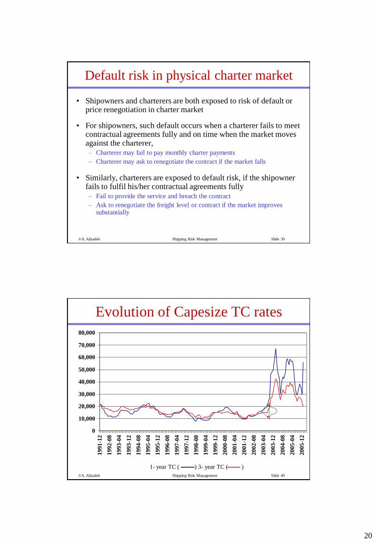
Evolution of Capesize TC rates

0

10,000

20,000

30,000

40,000

50,000

60,000

70,000

80,000

1991-1

2

1992-0

8

1993-0

4

1993-1

2

1994-0

8

1995-0

4

1995-1

2

1996-0

8

1997-0

4

1997-1

2

1998-0

8

1999-0

4

1999-1

2

2000-0

8

2001-0

4

2001-1

2

2002-0

8

2003-0

4

2003-1

2

2004-0

8

2005-0

4

2005-1

2

1- year TC ( ) 3- year TC ( )

21


Hedging Freight Default Risk

Using a credit default swap or option

• Shipowner can buy protection against possible charters default from a protection

seller (e.g. financial institution)

• This will cost a flat fee (e.g. $x/month)

• The pay off to the shipowner, when default occurs, can be the difference

between the current market rate for the remaining period of the original contract

and the compensation freight level (e.g. $25,000/day), which may or may not be

the physical contract TC rate

• The price of this product depends on– The creditworthiness of the charterer

– The duration of the contract

– Current market conditions (TC level, volatility, distance from the mean)

– The default swap compensation level (e.g. $22,000/day instead of $25,000)

– Interest rate


Hedging Freight Default Risk

Using a freight option

• Shipowner can buy protection against falling freight rates & possible charters

default by buying a put option on freight

• This will cost a flat fee (e.g. $x/day or month)

• The pay off to the shipowner, when freight rates drop below the strike price

(whether default occurs or not), will be the difference between the current

market rate and the strike price

– Put Option Payoff = max(0, X-FR)

• There might be several ways to set up such protection– Buying put option for every month over the life of the contract

– Buying a calendar put option for quarters or years

• The price of this product depends on– The duration of the contract – Current market conditions (TC level, volatility, distance from the mean)– The strike price level– Interest rate

22


There is no mathematical model to quantify such risk and

probability of default yet!

Therefore, important factors to consider when assessing the

credit risk and probability of default in physical charter market Counter party’s credit worthiness

Duration of contract

Current level of contract price (TC rate) in relation to its long term

mean

Probability of the market moving in different directions

Physical Freight Contract Default Risk


CreditMetrics (J.P. Morgan 1997)

23


Credit Risk Methodologies

CreditMetrics

CreditVaR

CreditRisk+ CreditPortfolioV

iew

Credit Monitor

JP Morgan CSFP McKinsey KMV Corp.

Credit Risk Market Value Default Losses Market Value Default Losses

Credit Events Credit Rating Change / Default

Default Credit Rating Change / Default

Continuous Default Probs

Risk Drivers Asset Values Default Rates Macro Factors Asset Values

Transition Probs Constant Stochastic Driven by Macro Factors

Driven by:

- EDF

- asset values

Correlation of credit events

Via asset values Via sectors Via factors Via asset values factor model

Recovery Rates Random (Beta) Loss given default

Random Random (Beta)

Computation Analytical/ Simulation

Analytical Simulation Analytical

CreditMetrics, CreditVaR is a registered trademark of J. P. Morgan, CreditRisk+ is a registered trademark of Credit Suisse Financial Products, CreditPortfolioView is a registered trademark of McKinsey and Co., Credit Monitor is a registered trademark of KMV Corporation.



• CreditMetrics, developed in 1997 by JP Morgan, a way of

measuring risk associated with default issues.

• From the CreditMetrics methodology one can calculate the

Credit Value at Risk (C-VaR), measured by standard deviation,

of a portfolio of assets over the required time horizon.

• Because of the risk of default the distribution of returns from a

portfolio exposed to credit risk is highly skewed.

• The distribution is far from being Normal. Thus ideas from simple

portfolio theory must be used with care.

• Although, it may not be a good absolute measure of risk in the

classical sense, the standard deviation is a good indicator of relative

risk between instruments or portfolios.

24


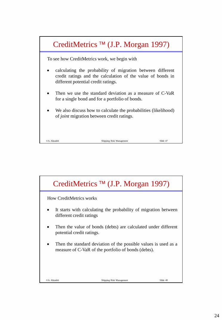
To see how CreditMetrics work, we begin with

calculating the probability of migration between different

credit ratings and the calculation of the value of bonds in

different potential credit ratings.

Then we use the standard deviation as a measure of C-VaR

for a single bond and for a portfolio of bonds.

We also discuss how to calculate the probabilities (likelihood)

of joint migration between credit ratings.



How CreditMetrics works

It starts with calculating the probability of migration between

different credit ratings

Then the value of bonds (debts) are calculated under different

potential credit ratings.

Then the standard deviation of the possible values is used as a

measure of C-VaR of the portfolio of bonds (debts).


25


Calculation of C-VaR

SeniorityCredit Rating Credit Spread

Recovery Rate in

DefaultMigration

Likelihoods

Value of Bond

in new Rating

Standard Deviation or Percentile Level for C-VaR

Flowchart of how Credit VaR is calculated using available

information


One-Year Transition Matrix

Year End Rating

Init Rate AAA AA A BBB BB B CCC Def

AAA 93.66 5.83 0.40 0.09 0.03 0.00 0.00 0.00

AA 0.66 91.72 6.94 0.49 0.06 0.09 0.02 0.01

A 0.07 2.25 91.76 5.18 0.49 0.20 0.01 0.04

BBB 0.03 0.26 4.83 89.24 4.44 0.81 0.16 0.24

BB 0.03 0.06 0.44 6.66 83.23 7.46 1.05 1.08

B 0.00 0.10 0.32 0.46 5.72 83.62 3.84 5.94

CCC 0.15 0.00 0.29 0.88 1.91 10.28 61.23 25.26

Def 0.00 0.00 0.00 0.00 0.00 0.00 0.00 100

Transition Probability Matrix of Bond Ratings after One Year

26


CreditMetrics (single bond)

Initial

Rating

Probability : End-Year Rating (%)

AAA AA A BBB BB B C D

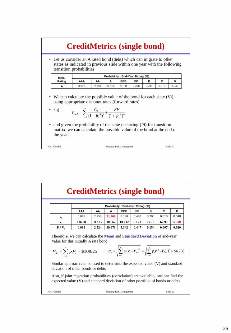
A 0.070 2.250 91.760 5.180 0.490 0.200 0.010 0.040

• Let us consider an A rated bond (debt) which can migrate to other states as indicated in previous slide within one year with the following transition probabilities

• We can calculate the possible value of the bond for each state (Vi), using appropriate discount rates (forward rates)

• e.g

• and given the probability of the state occurring (Pi) for transition matrix, we can calculate the possible value of the bond at the end of the year.

nA

n

n

iiA

i

iAA

fr

FV

fr

CV

)1()1(1

,



Therefore, we can calculate the Mean and Standard Deviation of end-year

Value for this initially A rate bond

Similar approach can be used to determine the expected value (V) and standard

deviation of other bonds or debts

Also, if joint migration probabilities (correlation) are available, one can find the

expected value (V) and standard deviation of other portfolio of bonds or debts

25.108$1

n

i

iim VpV 708.6$1

22

1

2

n

i

mii

n

i

miiv VVpVVp


AAA AA A BBB BB B C D

pi0.070 2.250 91.760 5.180 0.490 0.200 0.010 0.040

Vi 116.08 112.17 108.62 103.12 91.23 77.13 67.97 51.00

Pi* Vi 0.081 2.524 99.671 5.342 0.447 0.154 0.007 0.020

27


Revaluation at Risk Horizon (+1 year)

50 60 70 80 90 100 1100.000

0.025

0.050

0.075

0.100

0.900

Default CCCBB

BBB

A

AA

AAA

Fre

quen

cy

Distribution of 5-year A rated bond



Single Bond C-VaR

Percentile Level of C-VaR: A rated Bond

• Order values that debt (bond) may take from lowest to highest and thenadd up their joint likelihoods until these reach the 5% value (cumulativeprobability).

• Critical value closest to the 5% level gives $103.12, therefore 5%

C-VaR will beC-VaR = $5.128 (= Vm,p - $V5%tail = $108.25 - $103.12)

• Note that the distribution of expected values of bonds is not symmetric,

that is why it is better to use the critical values rather than SD when

estimating C-VaR, as we did


D C B BB BBB A AA AAA

pi 0.04 0.01 0.2 0.49 5.18 91.76 2.25 0.07

Vi 51 67.97 77.13 91.23 103.1 108.6 112.2 116.1

28


Single Bond C-VaR BB rated



pi 1.08 1.05 7.46 83.23 6.66 0.44 0.06 0.03

Vi 51.0 68.0 77.1 91.2 103.1 108.6 112.2 116.1

Percentile Level of C-VaR: BB rated Bond• Order values that debt (bond) may take from lowest to highest and then

add up their joint likelihoods until these reach the 1% value (cumulative probability).

Critical value closest to the 5% level gives $73.62, therefore 5%

C-VaR will be

C-VaR = $16.78 (= Vm,p – V5%tail = $90.394 - $73.62)

Note that the distribution of expected values of bonds is not symmetric, that is

why it is better to use the critical values rather than SD when estimating C-

VaR, as we did


CreditMetrics (two bonds)

• When there are more than one asset (bond) in our portfolio,

the final value of the portfolio depends on correlation

between credit movements of assets

• Consider the example of having the two bonds discussed

earlier in a portfolio

• We can use the end year values to calculate the value of

portfolio a the end of year

29




D 0.000 0.000 0.002 0.005 0.056 0.991 0.024 0.001

C 0.000 0.000 0.002 0.005 0.054 0.963 0.024 0.001

B 0.003 0.001 0.015 0.037 0.386 6.845 0.168 0.005

BB 0.033 0.008 0.166 0.408 4.311 76.372 1.873 0.058

BBB 0.003 0.001 0.013 0.033 0.345 6.111 0.150 0.005

A 0.000 0.000 0.001 0.002 0.023 0.404 0.010 0.000

AA 0.000 0.000 0.000 0.000 0.003 0.055 0.001 0.000

AAA 0.000 0.000 0.000 0.000 0.002 0.028 0.001 0.000

Probabilties of Rated Migrations

Pro

ba

bil

itie

s o

f

Ra

tin

g M

igra

tio

ns

Migration probabilities of the two initially “A” and “BB”

rated Bonds




D 102 118.97 128.13 142.23 154.1 159.6 163.2 167.1

C 118.97 135.94 145.1 159.2 171.07 176.57 180.17 184.07

B 128.13 145.1 154.26 168.36 180.23 185.73 189.33 193.23

BB 142.23 159.2 168.36 182.46 194.33 199.83 203.43 207.33

BBB 154.12 171.09 180.25 194.35 206.22 211.72 215.32 219.22

A 159.62 176.59 185.75 199.85 211.72 217.22 220.82 224.72

AA 163.17 180.14 189.3 203.4 215.27 220.77 224.37 228.27

AAA 167.08 184.05 193.21 207.31 219.18 224.68 228.28 232.18

Possible Values of an A Rated Bond

Po

ssib

le V

alu

es

of

a

BB

Ra

ted

Bo

nd

Value of the portfolio of the two initially “A” and “BB”

rated Bonds under the new possible ratings

30



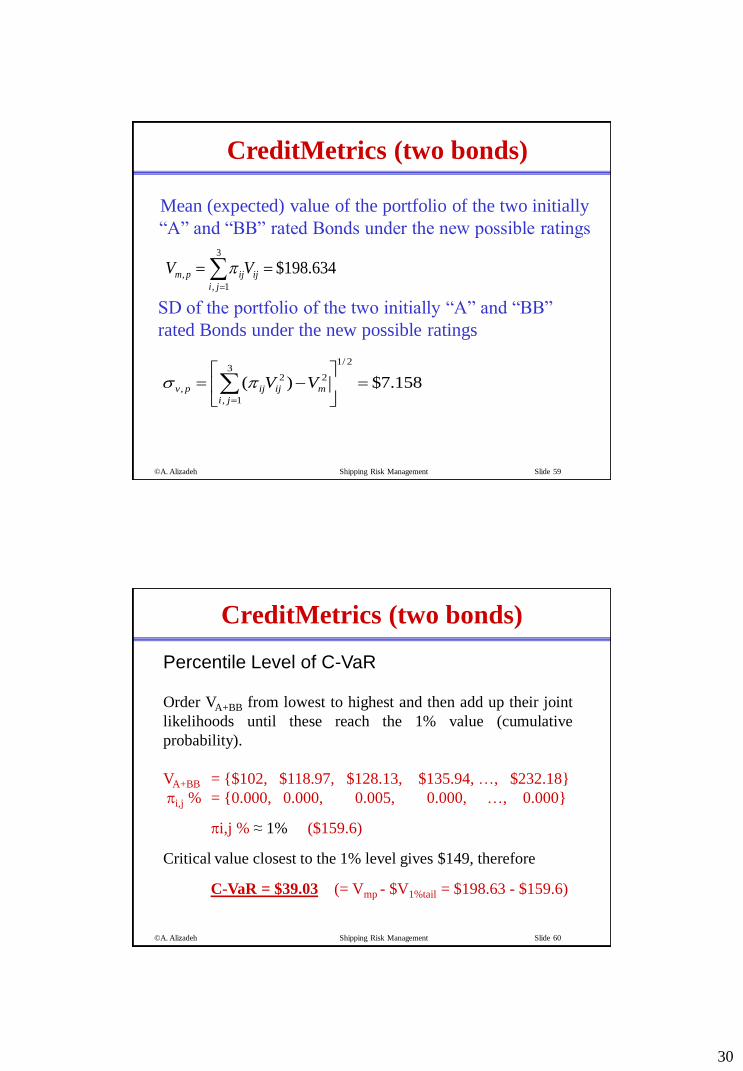
Mean (expected) value of the portfolio of the two initially

“A” and “BB” rated Bonds under the new possible ratings

634.198$3

1,

, ji

ijijpm VV

158.7$)(

2/13

1,

22

,

ji

mijijpv VV

SD of the portfolio of the two initially “A” and “BB”

rated Bonds under the new possible ratings



Percentile Level of C-VaR

Order VA+BB from lowest to highest and then add up their joint

likelihoods until these reach the 1% value (cumulative

probability).

VA+BB = {$102, $118.97, $128.13, $135.94, …, $232.18}

i,j % = {0.000, 0.000, 0.005, 0.000, …, 0.000}

i,j % ≈ 1% ($159.6)

Critical value closest to the 1% level gives $149, therefore

C-VaR = $39.03 (= Vmp - $V1%tail = $198.63 - $159.6)

31


Measuring Joint Credit Migration

• For a portfolio of debt (bonds), the joint credit migration

probabilities have to estimated as such migration (transitions)

might be correlated.

Measuring Joint Credit Migration

• The key element when dealing with calculation of C-VaR for a portfolio is

estimation of joint probabilities because

• Changes in credit ratings tend to move together with changes in

macroeconomic environment (recessions and expansions)

• correlations between credit rating changes even within sectors of the

economy and even within one country

• CreditMatrics deals with this problem using three basic approaches

• using historical data on joint credit migration

• using the asset value approach

• using bond spread data


Joint credit migration (historical data)

• This approach uses historical data to calculate credit migration

• For instance, a large sample of information on re-grading is collected over

time (e.g. over past 15 years)

• Then the sample correlation coefficients between annual up-grades and down

grades is calculated, e.g. (AB, B A), over the sample.

– E.g. every year out of 1000 A rated how many downgraded as B and out of 1000

B rates how many upgraded as A

• In order to have the full joint migration likelihoods a matrix of pairwise

correlation is constructed (e.g. for 8 ratings, we get 82 pairwise correlation)

– The advantage of this approach is that there is no need to make any assumption

about the distributional properties of ratings

– The disadvantage is that all companies within a rating class are treated the same

32


End of Slides


KMV Credit Monitor

33


KMV Credit Monitor & Merton’s Model

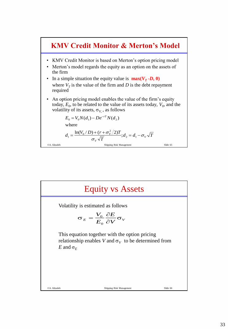
• KMV Credit Monitor is based on Merton’s option pricing model

• Merton’s model regards the equity as an option on the assets of the firm

• In a simple situation the equity value is max(VT -D, 0)

where VT is the value of the firm and D is the debt repayment required

• An option pricing model enables the value of the firm’s equity today, E0, to be related to the value of its assets today, V0, and the volatility of its assets, V, , as follows

TddT

TrDVd

dNDedNVE

V

V

V

rT

12

2

01

2100

;)2()/ln(

where

)()(


Equity vs Assets

E V

V

E

E

V 0

0

Volatility is estimated as follows

This equation together with the option pricing

relationship enables V and V to be determined from

E and E

34


Example

• Q: A company’s equity is $3 million and the volatility

of the equity is 80%. The risk-free rate is 5%, the debt

is $10 million and time to debt maturity is 1 year

• A: Solving the two equations yields V0=12.40 and

V=21.23%

– The probability of default is N(-d2) or 12.7%

– The market value of the debt is 9.40

– The present value of the promised payment is 9.51

– The expected loss is about 1.2%

– The recovery rate is 91%


The KMV Implementation of Merton’s Model

• Choose time horizon

• Calculate cumulative obligations to time horizon. This is termed

by KMV the “default point”. We denote it by D

• Use Merton’s model in reverse to calculate V0 and V

• Calculate distance to default

• The theoretical probability of default is N(-z)

• The distance to default is compared with actual default

experience and a one-to-one mapping of distance to default into

default probability is developed

VV

DV=z=

0

0Default toDistance

srm_lecture_6_2012.pdf

Documents

shipping company

default sources of credit

us shipping partners

atlas shipping files

us lloyds list

deloittes head of shipping

bankruptcy lloyds list

us bankruptcy court