Svensk Kärnbränslehantering ABSwedish Nuclear Fueland Waste Management Co

Box 250, SE-101 24 Stockholm Phone +46 8 459 84 00

R-13-25

SR-PSU Bedrock hydrogeologyGroundwater flow modelling methodology, setup and results

Magnus Odén, Svensk Kärnbränslehantering AB

Sven Follin, SF GeoLogic AB

Johan Öhman, Geosigma AB

Patrik Vidstrand, TerraSolve AB

April 2014

Tänd ett lager: P, R eller TR.

SR-PSU Bedrock hydrogeologyGroundwater flow modelling methodology, setup and results

Magnus Odén, Svensk Kärnbränslehantering AB

Sven Follin, SF GeoLogic AB

Johan Öhman, Geosigma AB

Patrik Vidstrand, TerraSolve AB

April 2014

ISSN 1402-3091

SKB R-13-25

ID 1372308

Keywords: Hydrogeology, Bedrock, Modelling, Temperate, Periglacial, Forsmark, SFR, Safety assessment.

A pdf version of this document can be downloaded from www.skb.se.

SKB R-13-25 3

Preface

The work presented in the current report describes the hydrogeological modelling for the fractured crystalline rock (bedrock) at the Forsmark-SFR site carried out as part of the SR-PSU project. The modelling has been planned, managed, and evaluated within the SKB hydrogeology discipline-spe-cific group HydroNet-SFR. The work and collaborative spirit of all HydroNet-SFR members is truly acknowledged.

Magnus OdénManager Hydrogeological Modelling SR-PSU

SKB R-13-25 5

Abstract

As a part of the license application for an extension of the existing repository for short-lived low and intermediate radioactive waste at the Forsmark-SFR site, the Swedish Nuclear Fuel and Waste Management Company (SKB) has undertaken site-scale groundwater flow modelling studies. The studies have been carried out within the SR-PSU project and represent two different climate condi-tions; temperate and periglacial. Periods with Glacial climate conditions are not a part of the hydro-geological modelling in SR-PSU for reasons described in Section 1.9.3. The groundwater flow simulations carried out contribute to the overall evaluation of the radiological safety of the geologi-cal disposal of short-lived low and intermediate radioactive waste in the bedrock at the Forsmark-SFR site.

The present report describes the groundwater flow modelling methodology, setup, and results. It is the primary reference for the conclusions drawn in the SR-PSU Main report concerning groundwa-ter flow in the bedrock during the two climate conditions. The detailed description of each modelling study is provided in separate documents (Öhman et al. (2014) and Vidstrand et al. (2014)). The main results and comparisons presented in the current report are summarised in the SR-PSU Main report.

6 SKB R-13-25

Sammanfattning

Som en del av ansökan för ett utbyggt SFR har Svensk Kärnbränslehantering (SKB) genomfört grundvattenmodelleringsstudier. Studierna har utförts inom projekt SR-PSU och hanterar grund-vattenströmning under perioder med två olika klimatförhållanden; tempererade och periglaciala. Grundvattenströmning under perioder med glaciala förhållanden har inte modellerats inom SR-PSU (se kapitel 1.9.3). Beräkningsresultaten från de utförda simuleringarna ingår i bedömningsunderlaget inom design och långsiktig säkerhet.

Föreliggande rapport sammanfattar modelleringsstudiernas uppställning, genomförande och resul-tat. Rapporten utgör huvudreferens för SR-PSU Main report vad gäller resultat som är kopplade till grundvattenströmning under de två klimatförhållandena. Detaljerade beskrivningar av de olika modelleringsstudierna finns redovisade i separata dokument (Öhman et al. (2014) och Vidstrand et al. (2014)). De väsentligaste resultaten och jämförelserna som redovisas i denna rapport samman-fattas i SR-PSU Main report.

SKB R-13-25 7

Contents

1 Introduction 91.1 Background of the SR-PSU project and its relation to the present report 91.2 The SR-PSU report hierarchy 91.3 Objectives 101.4 Relation to SDM-PSU 101.5 Outline of report 101.6 Nomenclature 101.7 Use of results from hydrogeological modelling within SR-PSU 121.8 Setting of the Forsmark-SFR site 121.9 Definiton of climate conditions and climate cases in SR-PSU 14

1.9.1 Climate domains 141.9.2 Climate cases 141.9.3 Handling in the hydrogeological modelling 16

2 Hydrogeological modelling within SDM-PSU 172.1 Primary data 17

2.1.1 Drilling campaigns 172.1.2 Hydrogeological borehole investigations 18

2.2 Hydrogeological model for the bedrock at the Forsmark-SFR site 192.3 Hydraulic properties of the bedrock in the SFR regional model domain 21

2.3.1 HCD 212.3.2 SBA 212.3.3 HRD 21

2.4 Geometric and hydraulic properties of the regolith in the SFR regional model domain 21

3 Groundwater flow modelling within SR-PSU 233.1 Excluded processes and considered performance measures 23

3.1.1 Excluded processes 233.1.2 Considered performance measures 25

3.2 Codes used in the flow modelling 253.2.1 DarcyTools 26

3.3 Modelling strategy, model domain and model set-up used for different climate domains 263.3.1 Boundary conditions 273.3.2 Hydrogeological domain 273.3.3 SFR regional domain 283.3.4 Geometry and handling of the existing SFR (SFR 1) and the

extension (SFR 3) in the groundwater flow model 283.3.5 Temperate climate domain 313.3.6 Periglacial climate domain 313.3.7 Modelling of groundwater flow to potential domestic water wells

5000 AD 33

4 Temperate climate domain 354.1 Overview 354.2 Objectives 354.3 Model parameterisation 36

4.3.1 Regolith 364.3.2 Bedrock inside the SFR Regional domain 374.3.3 Bedrock outside SFR Regional domain 404.3.4 Model variants in SR-PSU 41

4.4 Boundary conditions 424.4.1 Top boundary 424.4.2 Lakes and rivers 42

8 SKB R-13-25

4.5 Results from the modelling of temperate climate conditions 434.5.1 Cross flow 444.5.2 Median values of Q, Fr, tw,r, and Lr 474.5.3 Exit locations 494.5.4 Discharge to biosphere object 157_2 514.5.5 Flow-related transport resistance 534.5.6 Advective travel time 564.5.7 Path length 59

5 Periglacial climate domain 635.1 Overview 635.2 Scope and objectives 645.3 Model parameterisation 65

5.3.1 State laws 655.3.2 Regolith 655.3.3 Bedrock inside SFR Regional domain 655.3.4 Bedrock outside SFR Regional domain 665.3.5 Model variants assessed in the periglacial climate condition 66

5.4 Boundary conditions 675.4.1 Lateral and bottom boundary 675.4.2 Top boundary 67

5.5 Results 695.5.1 Cross flow 695.5.2 Particle tracking 715.5.3 Exit locations 715.5.4 Flow-related transport resistance 725.5.5 Advective travel time 745.5.6 Path length 76

6 Integration of climate conditions and disciplines 796.1 Consistency between models used for flow modeling during temperate and

periglacial climate conditions 796.2 Use of hydrogeological properties and results in other disciplines within

SR-PSU 806.2.1 Near field 806.2.2 Biosphere analyses 806.2.3 Surface hydrology 806.2.4 Far field Radionuclide transport 806.2.5 Geochemical analyses 80

7 Summary and conclusions 81

References 83

Appendix A DarcyTools 87

SKB R-13-25 9

1 Introduction

1.1 Background of the SR-PSU project and its relation to the present report

As a part of the license application for an extension of the existing repository for short-lived low- and intermediate-level radioactive waste (SFR) at the Forsmark-SFR site, the Swedish Nuclear Fuel and Waste Management Company (SKB) has performed the SFR extension project (PSU). The objective of SR-PSU is to assess the radiological safety of the entire SFR-repository after closure. The existing repository facility is in SR-PSU denoted by SFR 1 and the planned facility extension by SFR 3.

SR-PSU comprises a main report, here denoted the SR-PSU Main report, and a set of primary references. These include among others, with specific relevance for the current report, the Climate report, Data report, Geosphere process report, Initial state report and Radionuclide transport report. In addition, there are a number of additional references such as the work presented here.

The present report serves as a reference for the Data report and Input data report concerning hydrogeological results used within SR-PSU. This means that the report serves as a primary refer-ence for the different hydrogeological model applications within the SR-PSU project as well as for the SR-PSU Main report. It is noted that hydrogeological conclusions in a SR-PSU-specific context are drawn in the SR-PSU Main report. The outline and content of the present report are much influ-enced by the hydrogeological synthesis report in the safety assessment for the spent fuel repository, SR-Site (Selroos and Follin 2010).

1.2 The SR-PSU report hierarchyThe SR-PSU project is reported in a series of SKB reports, which includes a main report and a set of primary references that are referred to by abbreviated names in the SR-PSU reporting. The primary references and the names used (in bold) when referring to them in this and other SR-PSU reports are listed in Table 1-1. In addition to the primary references, the safety assessment is based on a large number of background reports and other references.

Table 1-1. Primary references in the SR-PSU project; FEP stands for features, events and processes, and FHA is short for future human actions.

Report number Short name used when referred to in the text

Full title

TR-14-01 SR-PSU Main report Safety analysis for SFR. Long-term safety. Main report for the safety assessment SR-PSU.

TR-14-02 Initial state report Initial state report for the safety assessment SR-PSU.TR-14-03 Waste process report Waste form and packaging process report for the safety assessment

SR-PSU.TR-14-04 Barrier process report Engineered barrier process report for the safety assessment

SR-PSU.TR-14-05 Geosphere process report Geosphere process report for the safety assessment SR-PSU.TR-14-06 Biosphere synthesis report Biosphere synthesis report for the safety assessment SR-PSU.TR-14-07 FEP report FEP report for the safety assessment SR-PSU.TR-14-08 FHA report Handling of future human actions in the safety assessment SR-PSU.TR-14-09 Radionuclide transport report Radionuclide transport and dose calculations for the safety assessment

SR-PSU.TR-14-10 Data report Data report for the safety assessment SR-PSU.TR-14-11 Model summary report Model summary report for the safety assessment SR-PSU.TR-14-12 Input data report Input data report for the safety assessment SR-PSU.TR-13-05 Climate report Climate and climate related issues for the safety assessment SR-PSU.

10 SKB R-13-25

1.3 ObjectivesThe main objectives of the current report are the following.

• Provide an integrated account of the hydrogeological modelling for the bedrock carried out as part of SR-PSU.

• Summarise the hydrogeological modelling strategy and model setups for the bedrock used in SR-PSU; especially how the studied climate conditions, scales, and model tools relate to each other.

• Provide a rationale for the hydrogeological base cases and variants defined for the hydrogeo-logical model applications that have been studied.

• Provide an evaluation and discussion of the results obtained in the hydrogeological modelling.

1.4 Relation to SDM-PSUThe hydrogeological description in SR-PSU is based on the site-descriptive model, SDM-PSU, pre-pared at the completion of the associated SFR site investigation (SKB 2013). The hydrogeological conceptualisation and the methods used for flow model parameterisation are in principle identical to that of the site-descriptive model SDM-Site (SKB 2008b).

1.5 Outline of reportThe outline of the report is as follows: Chapter 1 presents the background and objectives of the report as well as a description of how the results of the hydrogeological modelling are used in subsequent analyses within the SR-PSU project. Chapter 2 is a brief summary of the conceptual hydrogeological model developed in SDM-PSU, which is the primary input used in the groundwater flow modelling carried out by Öhman et al. (2014) and Vidstrand et al. (2014). Chapter 3 describes the flow modelling methodology as well as the time periods analysed and model domains utilised in SR-PSU. Chapters 4 and 5 present the two climate domains that were studied. Within each chap-ter, the analyses requested by SR-PSU are provided, and the base case and alternatives used in the modelling studies are presented along with the results. Chapter 6 presents the integration of the two climate conditions and the recommended use of hydrogeological properties and results in other disci-plines within SR-PSU. Chapter 7 provides a summary of the main results for further use in SR-PSU.

1.6 NomenclatureThis report contains several terms and acronyms that are rarely used outside SKB work and makes several references to site-specific deformation zones. To facilitate the readability of the report these are listed in Table 1-2.

Table 1-2. Terminology, acronyms and structures referred to in the report.

Central notations used in the hydrogeological modelling

SDM-Site Forsmark The site where the geological repository of spent fuel at Forsmark is planned (SKB 2008b).Forsmark-SFR site The site where the existing SFR facility is located, about 2 km north of the site selected for

the final repository for spent nuclear fuel (SKB 2013).Sheet joint (SDM-Site Forsmark)

Sheet joints (or exfoliation joints) are sub-horizontal fracture systems often initiated by stress release. In SDM-Site Forsmark, sheet joints locally exert strong directional control on groundwater flow and contaminant transport (Follin 2008).

Shallow bedrock aquifer (SDM-Site Forsmark)

Flow model concept used to characterise the uppermost c. 150 m of the bedrock in SDM-Site Forsmark. This realm of rock is hydraulically dominated by large, sub-horizontal, transmissive structures recognised as sheet joints. In SDM-Site Forsmark, the shallow bedrock was modelled as three horizons with spatially varying transmissivity. The three horizons were labelled “shallow bedrock aquifer”.

SKB R-13-25 11

Central notations used in the hydrogeological modelling

SBA structure (SDM-PSU) Network of predominantly sub-horizontal fractures of elevated transmissivity in the Fors mark-SFR site. Inside the SFR Regional model domain, see Figure 2-1, eight such net works of fractures are represented by planes for deterministic modelling purposes in the uppermost 200 m bedrock. These are labelled SBA1 to SBA8.The term SBA structure is used in the context of SFR to emphasise that these structures are of different (lesser) size and of less hydraulic significance as compared to the shallow bedrock aquifer modelled in SDM-Site Forsmark.

Unresolved PDZ Borehole intervals geologically interpreted to have “deformation-zone like characteristics” are referred to as Possible Deformation Zones (PDZ). In the geological modelling, deter-ministic structures (ZFMxxx) are modelled by linking PDZs to surface lineaments. Remain-ing PDZs, which cannot be linked to lineaments, are referred to as “Unresolved PDZs”.

Central block (CB) The geological model developed on behalf of SDM-PSU (Curtis et al. 2011) defines a tec-tonic volume at the centre of the SFR Regional domain, enclosed by the so-called Northern and Southern boundary belts.In the hydrogeological modelling, no distinct boundaries have been defined between the Central block and the rock mass affected by the bounding belts; the transition seems to be gradual (Öhman et al. 2012).

Northern boundary belt (NBB)

The geological model (Curtis et al. 2011) defines a northern belt of large deformation zones acting as a geological boundary for the Central block where the repository facilities are located. The key deformation zones behind the concept of the Northern boundary belt are ZFMNW0805A/B.

Southern boundary belt (SBB)

The geological model (Curtis et al. 2011) defines a southern belt of large deformation zones acting as a geological boundary for the Central block where the repository facilities are located. The key deformation zones behind the concept of the Southern boundary belt are ZFMWNW0001 (the Singö deformation zone), and splays.

Acronym Stands for Explanation

DEM Digital Elevation Model Topographic model for the Forsmark area, covering both land and seafloor with a spatial resolution of 20 m in the horizontal plane.

DFN Discrete Fracture Network

In DFN modelling, fractures, and fracture flow, are typically resolved as a network of square geometric features of different sizes and hydraulic properties.

ECPM Equivalent Continuous Porous Medium

A flow modelling concept, where the hydraulic properties of a conductive fracture network are approximated by those of a continuous porous medium. Thus, an ECPM model does not resolve explicit fracture flow, and hence is useful in large- scale simulations and on site-scale if fractures are resolved with fine enough discretization.

GEHYCO GEnerate HYdraulic COnductivity

DarcyTools is a computer code for simulation of flow and transport in porous and/or fractured media.GEHYCO is the module in DarcyTools used to translate a hydraulic DFN into an ECPM (Svensson et al. 2010).

HCD Hydraulic Conductor Domain

Hydraulic representation of identified deterministic deformation zones (Rhén et al. 2003).

HRD Hydraulic Rock mass Domain

Hydraulic representation of the stochastic fractures between deformation zones (Rhén et al. 2003).

HSD Hydraulic Soil Domain Hydraulic representation of the regolith (Quaternary deposits mainly) (Rhén et al. 2003).

PDZ Possible Deformation Zone

A borehole section that has geologically been interpreted to have “deformation-zone like characteristics” (i.e. a possible deformation zone intercept). In the geological modelling, deterministic structures (ZFMxxx) are modelled in 3D by linking PDZs to surface lineaments. Remaining PDZs, which cannot be linked to lineaments, are referred to as “Unresolved PDZs”.

SDM Site-Descriptive Model A multi-disciplinary description of the site, including both qualitative and quantita-tive information, that is based on both direct observations and modelling studies.

SFR SlutFörvaret för kortlivat Radioaktivt avfall

The existing final repository for short-lived radioactive waste.

SKB Svensk Kärnbränsle-hantering AB

The Swedish Nuclear Fuel and Waste Management Company.

ZFM Deformation one in the Forsmark area

Deterministically modelled deformation zone in the geological model are given unique labels beginning with “ZFM”. These are modelled by linking borehole intercepts with “deformation-zone like characteristics” to surface lineaments (cf. the acronym PDZ).

12 SKB R-13-25

Key deformation zones (Deterministic structures of the Geological model SFR v 1.0)

Alternatively known as: (Structures in early SFR models)

ZFMWNW0001 Core of the bounding Southern deformation zone belt. Singö deformation zoneZFMNW0805A/B Deformations zones that constitute the Northern

boundary belt.Zone 8

ZFMNNW1034 Deformation zone of high transmissivity that cuts across the wedge defined by the intersection of the Northern and Southern boundary belts.

Not modelled in previous SFR models

ZFM871 Gently dipping deformation zone below the existing repository facility (SFR 1).

Zone H2

ZFMENE3115 A deformation zone that terminates ZFM871 to the southeast.

Not modelled in previous SFR models

ZFMNE0870 Low-transmissive deformation zone parallel to the access tunnels.

Zone 9

ZFMNNE0869 High-transmissive deformation zone intersecting access tunnels .

Zone 3

ZFMNNW1209 A deformation zone that intersects the SFR 1 rock vaults Zone 6ZFMWNW1035 A deformation zone that occurs at the northern rim of the

Sothern Belt.Zone 1

1.7 Use of results from hydrogeological modelling within SR-PSUThe hydrogeological modelling of the bedrock at the Forsmark-SFR site serves several assessment activities within SR-PSU. First, the results are descriptions of the hydrogeological conditions during temperate and periglacial climate conditions. These descriptions are required for demonstrating a good understanding of the characteristics of the site at the present day and how those conditions change in the future. Second, various sets of results are exported to other disciplines such as radio-nuclide transport calculations, hydrogeochemistry, and biosphere analyses. The specific uses made of the hydrogeological results are summarised in Chapter 7.

The hydrogeological analyses within SR-PSU devote particular attention to the evolution of hydro-logical conditions driven by changes in the climate and surface system. For instance, if the ongoing shoreline displacement continues as forecast, the location of the Forsmark-SFR site will change from a discharge area to a recharge area at approximately 3000 AD. Hence, the geosphere needs to be assessed both in terms of its effect on the engineered barriers as well as its own performance as a barrier. In other words, groundwater flow from the surface (recharge areas) to the repository, and from the repository to the surface (discharge areas) have to be studied.

Given the hydrological evolution, the geosphere is a dynamic system from both the hydrogeologi-cal and hydrogeochemical points of view. The present report tries to convey this notion of a dynamic system, i.e. it illustrates how the effects of temperate and periglacial climate conditions have been conceptualised in numerical models. Furthermore, simulations investigating various hydrogeological uncertainties are described.

1.8 Setting of the Forsmark-SFR siteThe Forsmark-SFR site is located in northern Uppland within the municipality of Östhammar, about 120 km north of Stockholm (Figure 1-1). The Forsmark-SFR site is located about 2 km north of the site selected for the final repository for spent nuclear fuel (SDM-Site Forsmark).

The current ground surface in the Forsmark region forms a part of the sub-Cambrian peneplain in south-eastern Sweden. This peneplain represents a relatively flat topographic surface with a gentle dip towards the east that formed more than 540 million years ago. The Forsmark region is characterised by small-scale topography at low elevation (Figure 1-2). The whole area is located below the highest coastline associated with the last glaciation, Weichsel, and large parts of the area emerged from the Baltic Sea only during the last 2,000 years. Both the flat topography and the still ongoing shoreline displacement of about 6 mm per year strongly influence the current landscape. Sea bottoms are continuously trans-formed into new terrestrial areas or freshwater lakes, and lakes and wetlands are successively covered

SKB R-13-25 13

by peat. Most of the Forsmark-SFR site is currently covered by brackish sea water (Figure 1-3), but the seafloor will continue to rise and the seabed above Forsmark-SFR site will be at the shoreline within about 1,000 years, i.e. the Forsmark-SFR site is currently covered by about 6 m of sea water.

The elevation of the existing repository facility at the Forsmark-SFR site, SFR 1, ranges between c. –70 m and –140 m. The elevation of the planned facility extension, SFR 3, ranges between c.–120 m and –140 m.

Figure 1-1. Map of the Forsmark-SFR site showing the location of the existing SFR facility (SFR 1) and the suggested area for the SFR extension (SFR 3). The strip of land running above the two SFR 1 tunnels is referred to as the ‘SFR Pier’ in this report.

Figure 1-2. Photograph showing the flat topography and the low-gradient shoreline with recently isolated bays due to land uplift.

14 SKB R-13-25

1.9 Definiton of climate conditions and climate cases in SR-PSU1.9.1 Climate domainsIn the Climate report three different climate domains are identified to describe the climate evolution for the Forsmark-SFR site:

• The temperate climate domain

• The periglacial climate domain

• The glacial climate domain

The purpose of identifying climate domains is to create a framework for the assessment of issues of importance for repository safety associated with particular climatically determined environments that may occur in Sweden in the future.

The temperate climate domain is defined as regions without permafrost or presence of ice sheets. It is dominated by a temperate climate in a broad sense, with cold winters and either cold or warm summers. Precipitation may fall at any time of the year. The precipitation falls either as rain or snow. The temperate climate domain has the warmest climate of the three climate domains. Within the temperate climate domain, a site may also at times be submerged by the sea. Climates dominated by global warming due to enhanced atmospheric greenhouse gas concentrations are also included in the temperate climate domain.

The periglacial climate domain is defined strictly as regions that are subjected to permafrost. Further more, the periglacial climate domain is a cold region but without the presence of an ice sheet. In this climate domain, permafrost occurs either in sporadic (less than 50% spatial coverage), discontinuous (between 50 and 90% coverage), or continuous form (more than 90% coverage).

The glacial climate domain is defined as regions that are covered by glaciers or ice sheets. In gen-eral, the glacial climate domain has the coldest climate of the three climate domains. Precipitation normally falls as snow in this climate domain.

1.9.2 Climate casesBased on the scientific knowledge on the influence of enhanced atmospheric greenhouse gas con-centrations and low-amplitude insolation variability in the next tens of thousands of years (see the

Figure 1-3. Figure showing the existing SFR facility (SFR 1) and the suggested area (yellow) for the SFR extension (SFR 3) in the foreground and the Forsmark nuclear power plant buildings in the background. The distance from SFR 1 to the shoreline is about 2 km. The strip of land (a man made wave breaker) running above the SFR 1 tunnels is referred to as the ‘SFR Pier’ in this report, cf. Figure 1-1.

SKB R-13-25 15

Climate report) a set of three climate cases were defined. These represent different levels of cumu-lative carbon emissions due to human activities:

• The Global warming climate case represents medium-level carbon emissions.

• The Early periglacial climate case represents low-level carbon emissions.

• The Extended global warming climate case represents high-level carbon emissions due to human activities.

These climate cases consist of a 100,000 year long succession of temperate and periglacial climate conditions in Forsmark, see example of the Early periglacial climate case in Figure 1-4.

To supplement this range of future climate developments, a climate case based on a reconstruction of the last glacial cycle was defined. The Weichselian glacial cycle climate case represents a climate development dominated by natural variability as manifested during the past c. 100 ka. This climate case consist of a 100,000 year long succession of temperate, periglacial and glacial climate conditions in Forsmark. Current scientific understanding (Climate report) indicates that the current inter-glacial (warm period) will persist longer than the previous interglacial due to the human-induced elevated atmospheric greenhouse gas concentrations. Therefore, the climate evolution given by the Weichselian glacial cycle climate case is not judged to be representative for the next 100,000 years in Forsmark. In addition, the climate cases also describe periods with submerged conditions, occurring after major glacial phases due to isostatic depression of the crust and to sea-level changes. Further, since the SFR repository is currently located below sea level, all climate cases start with a submerged period. Figure 1-5 illustrates, from a hydrogeological perspective, the conceptual models of the climate con-ditions relevant for the Forsmark area. Based on these conceptual models, the numerical groundwater model is developed in order to include all essential processes, governing the recharge and discharge of water at the top boundary.

Figure 1-4. Evolution of climate-related conditions at Forsmark as a time series of climate domains and submerged periods for the early periglacial climate case (Figure 4-5 in the Climate report).

Figure 1-5. Conceptual illustration of the hydrological system for different climate conditions. Observe that illustrations are not to scale.

0 10 20 30 40 50 60 70 80 90 100

TemperatePeriglacialGlacial basal frozen basal melting

Submergedconditions

Climate domainsInsolation minimum

17 ka AP

Time (ka AP)

Early periglacialclimate case

16 SKB R-13-25

1.9.3 Handling in the hydrogeological modellingThe overall objective of groundwater flow modelling within SR-PSU is to assess the effects of selected climate domains on site hydrogeological conditions, specifically distribution of ground-water flow, in the presence of a closed repository.

Glacial conditions cannot be completely ruled out for the 100,000 year long SR-PSU assessment period, as indicated in the Weichselian climate case (Climate report). However, it is very likely that a glacial period at Forsmark is preceded by periods of periglacial conditions with permafrost, as illustrated in the Weichselian climate case. The possible timing of the first period of periglacial conditions is however described by the Early periglacial climate case and the Global warming cli-mate case, see the Climate report. In these climate cases it cannot be excluded that the SFR con-crete barriers are degraded by freezing by around 50 ka AP (SR-PSU Main report). In line with the above information, it is in SR-PSU assumed that the concrete barriers are degraded, by freezing and/or other processes, at the time of ice sheet overriding in the Weichselian climate case.

In addition, if an ice sheet were to advance over the SFR facility, this would most likely occur over a periglacial fore field with permafrost. The permafrost depth may well confine the entire shallow SFR facility. This would minimize the possibility of through flow during the passage of the ice front, which is by far the period of largest potential increase of head gradient during glacial conditions (Vidstrand et al. 2012). As the frozen ground successively melts beneath the ice sheet, the head gra-dient will also diminish significantly (Vidstrand et al. 2010) and the possibility for discharge will be confined to taliks beyond the ice margin and thus far away from the repository location. During a retreat phase from a major glaciation, the fore field at Forsmark will be submerged beneath a melt water lake or Baltic Sea stage. In this case, the ice sheet profile near the margin will be considerably less steep than during the advance and hence the flows will exhibit relatively minor increases and the discharge will occur into the melt water lake with a large potential for dilution effects.

In line with the above reasoning, the hydrogeological modelling handled in this report focuses on the temperate and periglacial climate domains. The glacial climate domain is not a part of the hydro-geological modelling in SR-PSU. The SFR tunnels are assumed to be immediately filled with water upon closure. Hence, the excavation and operational phases, when the tunnels will be at atmospheric pressure, are not a part of the hydrogeological modelling in SR-PSU.

SKB R-13-25 17

2 Hydrogeological modelling within SDM-PSU

SKB (2013) presents the integrated understanding of the Forsmark-SFR site (labelled SDM-PSU) at the completion of the SFR site investigation. The hydrogeological modelling carried out in sup-port of SDM-PSU is described in detail in Öhman et al. (2012, 2013). This chapter describes briefly the hydrogeological model of the Forsmark-SFR site, primary data acquired for the bedrock, and hydraulic characteristics of the delineated hydraulic domains.

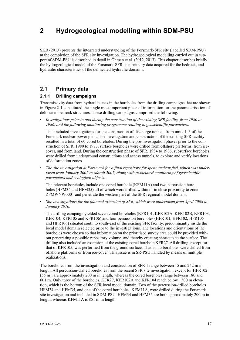
2.1 Primary data2.1.1 Drilling campaignsTransmissivity data from hydraulic tests in the boreholes from the drilling campaigns that are shown in Figure 2-1 constituted the single most important piece of information for the parameterisation of delineated bedrock structures. These drilling campaigns comprised the following.

• Investigations prior to and during the construction of the existing SFR facility, from 1980 to 1986, and the following monitoring programme relating to geoscientific parameters.

This included investigations for the construction of discharge tunnels from units 1–3 of the Forsmark nuclear power plant. The investigation and construction of the existing SFR facility resulted in a total of 60 cored boreholes. During the pre-investigation phases prior to the con-struction of SFR, 1980 to 1983, surface boreholes were drilled from offshore platforms, from ice-cover, and from land. During the construction phase of SFR, 1984 to 1986, subsurface boreholes were drilled from underground constructions and access tunnels, to explore and verify locations of deformation zones.

• The site investigation at Forsmark for a final repository for spent nuclear fuel, which was under-taken from January 2002 to March 2007, along with associated monitoring of geoscientific parameters and ecological objects.

The relevant boreholes include one cored borehole (KFM11A) and two percussion bore-holes (HFM34 and HFM35) all of which were drilled within or in close proximity to zone ZFMWNW0001 and penetrate the western part of the SFR regional model domain.

• Site investigations for the planned extension of SFR, which were undertaken from April 2008 to January 2010.

The drilling campaign yielded seven cored boreholes (KFR101, KFR102A, KFR102B, KFR103, KFR104, KFR105 and KFR106) and four percussion boreholes (HFR101, HFR102, HFR105 and HFR106) situated south to south-east of the existing SFR facility, predominantly inside the local model domain selected prior to the investigations. The locations and orientations of the boreholes were chosen so that information on the prioritised survey area could be provided with-out penetrating a possible repository volume, and thereby creating shortcuts to the surface. The drilling also included an extension of the existing cored borehole KFR27. All drilling, except for that of KFR105, was performed from the ground surface. That is, no boreholes were drilled from offshore platforms or from ice-cover. This issue is in SR-PSU handled by means of multiple realizations.

The boreholes from the investigation and construction of SFR 1 range between 15 and 242 m in length. All percussion-drilled boreholes from the recent SFR site investigation, except for HFR102 (55 m), are approximately 200 m in length, whereas the cored boreholes range between 180 and 601 m. Only three of the boreholes, KFR27, KFR102A and KFR104 reach below −300 m eleva-tion, which is the bottom of the SFR local model domain. Two of the percussion-drilled boreholes HFM34 and HFM35, and one of the cored boreholes, KFM11A, were drilled during the Forsmark site investigation and included in SDM-PSU. HFM34 and HFM35 are both approximately 200 m in length, whereas KFM11A is 851 m in length.

18 SKB R-13-25

2.1.2 Hydrogeological borehole investigationsExcept for HFR102, all percussion-drilled boreholes were investigated with the so-called HTHB-equipment, designed to perform combined pump tests and impeller flow logging in open percussion-drilled boreholes. HFR102 was investigated by means of an injection test. The cored boreholes from the SFR site investigation, including KFM11A, were all investigated by means of difference flow logging using the Posiva Flow Log (PFL) device.

The single-hole transmissivity data available from the older boreholes drilled in conjunction with the construction of SFR have been measured by four different methods:

• falling head (FH),

• pressure build-up (BU),

• steady-state injection (PH), and

• transient injection (TI).

Figure 2-1. Map visualising the borehole coverage within the model area showing the horizontal component of inclined boreholes. Boreholes are colour coded by investigation project/period and according to type; cored boreholes (KFRXX) are shown as filled trajectories ; the dotted trajectories represent percussion-drilled boreholes (HFRXX).

SKB R-13-25 19

Altogether, there are 1,122 tested sections distributed among 45 boreholes, but the data are of vary-ing quality; the tests have been evaluated with different test methods, at different test-scales, and under different test durations. Consequently, the data have different detection limits. However, most transmissivity data are measured over 3 m borehole sections and have a high detection limit, around 5·10–8 m2/s. Pressure build-up tests and transient injection tests have the longest durations (several hours), resulting in lower detection limits; unfortunately such data are relatively rare and have large variation in test scale. The falling-head and steady-state injection data had test durations of a few min-utes only; they comprise a large sample size of consistent test scale (3 m sections). Falling-head data have an overall low confidence in relation to the other data types (Carlsson et al. 1986). In total, about 40% of the tested sections fall below the detection limit. The hydraulic data set underwent a screen-ing process, in which 179 overlapping data, erroneous data, and inconsistent data were excluded, as described in Öhman and Follin (2010).

Two short interference tests were performed in the site investigation for the SFR extension; a pumping test in HFR101 and opening of the underground borehole KFR105. In addition to these tests, interferences from borehole activities that cause hydraulic responses, like drilling and nitro-gen flushing, were analysed and evaluated by Walger et al. (2010). The evaluation of interference tests involved estimations of hydraulic diffusivity, normalised drawdown and boundary condition interpretations for responding observation sections. The evaluation of drilling responses involved a qualitative classification of the responses at different drilling depths and a quantitative estimation of hydraulic diffusivity between the drilled borehole and the observation section.

A number of interference tests were also performed during 1985 to 1987 in the boreholes from the investigation and construction of SFR, to provide insight into the connectivity between zones (Axelsson et al. 2002). The responses have only been used qualitatively; classed as direct response, indirect response and no response (an indirect response implies that the observation borehole and the source borehole are located in different structures but are hydraulically connected).

2.2 Hydrogeological model for the bedrock at the Forsmark-SFR site

The conceptual hydrogeological model, version 1.0, for the bedrock contained inside the SFR regional model domain is sketched in 3D in Figure 2-2. In summary, this model encompasses:

• Three major tectonic units defined in the bedrock geological model version 1.0 (Curtis et al. 2011): the Southern boundary belt, the Central block, and the Northern boundary belt.

• Forty hydraulic conductor domains (abbrev. HCDs) coinciding with deformation zones, 21 of which have been assigned a high confidence of existence. Three of the 40 deformation zones are gently dipping; all other deformation zones are either vertical or steeply dipping and follow the orientation sets identified by their geological character in the earlier model for the deformation zones at Forsmark (Stephens et al. 2007).

• Eight gently dipping shallow bedrock aquifer structures (abbrev. SBA) representing potential net-works of predominantly sub-horizontal fractures of elevated intensity and transmissivity within the investigated SFR area. In the flow model, the eight networks are treated deterministically and implemented as planes in the uppermost 200 m bedrock.

• Three hydraulic rock mass domains (abbrev. HRD): Shallow bedrock HRD, Repository level HRD and Deep bedrock HRD. Each HRD consists of two types of stochastic features: 1) unresolved possible deformation zones (abbrev. PDZ), and 2) discrete fracture networks (abbrev. DFN). The unresolved PDZ realizations are spatially constrained to occur along the structural wedge defined by the Northern boundary belt, deformation zone ZFMNNW1034, and the Southern boundary belt. The unconditional DFN realizations represent the background fracturing between deforma-tion zones within the SFR regional model.

Figure 2-3 shows example visualisations of the hydraulic domains used to model the bedrock (HCD, SBA, HRD (i.e. Unresolved PDZ, and DFNs).

20 SKB R-13-25

Figure 2-2. Side view facing west showing the conceptual model of hydraulic, the interconnected flowing fracture network, and potential flow paths towards the Central block due to inflow to the existing SFR facility or borehole pumping during the SFR site investigation. The hydraulic domains are defined in Section 4.1. The vertical deformation zones (HCDs) contained in the Northern and Southern boundary belts connect the Baltic Sea to the bedrock and may thus act as potential positive hydraulic boundaries for inflow to the planned SFR extension. However, flow from the bounding belts towards the Central block is partly constrained by hydraulic chokes. The horizontal and vertical dimensions of this illustration are approximately 1.5 km and 1.1 km, respectively. The strip of land is the ‘SFR Pier’, cf. Figure 1-1.

Figure 2-3. Example visualisation of the hydraulic domains considered for the bedrock at the Forsmark-SFR site in SDM-PSU; a HCDs, b SBAs, c Unresolved PDZs, and d DFN.

Northern boundary belt (ZFMNNW1034)

Southern boundary belt Hydraulic Conductor

Domain (HCD)

Sediments (HSD)Shallow Domain (HRD)

Deep Domain (HRD)

Hydraulicchoke

Constrainedver�cal flow

CentralBlock

Deep regional flow paths

Inland SBA groundwater

Repository Domain (HRD)

SBA structure

Unresolved PDZ

SFR Pier

SKB R-13-25 21

2.3 Hydraulic properties of the bedrock in the SFR regional model domain

The borehole investigations provide detailed information about the heterogeneity in bedrock prop-erties. The delineated depth trends and lateral variations in transmissivity are studied by means of a hydrogeological base case and a few model variants, see Chapters 3-5. The references to the data used for hydraulic parameterisation of the hydraulic domains shown in Figure 2-3 are listed below.

2.3.1 HCDThe deformation zone model developed by Curtis et al. (2011) is used for HCD modelling inside the SFR regional model domain (Figure 2-1). Outside this domain, the deformation zone model derived for SDM-Site Forsmark by Stephens et al. (2007) is used (see Chapter 3).

The deformation zones are tessellated into smaller segments in order to allow for spatial variability in transmissivity, cf. Eq. 7-3 in SKB (2013). Input data inside the SFR regional model domain are compiled in Appendix 6 in SKB (2013). Outside this domain, input data are imported from SR-Site, see e.g. Joyce et al. (2010).

2.3.2 SBAThe geometric and hydraulic descriptions of the SBA structures are provided in Appendices B and H in Öhman et al. (2012).

2.3.3 HRDUnresolved PDZStochastic realisations of unresolved PDZs are according to the modelling procedure and property assignment described in Öhman et al. (2012, Appendix A).

DFNThe generation of discrete fracture network realisations for the background rock is based on the properties provided in Appendix 5 in SKB (2013). These properties are used throughout the SFR regional model area. Outside the regional SFR model area and the area modelled in SDM-Site, the generation of discrete fracture network realisations is based on the model setup described in Öhman and Follin (2010, Appendix A).

2.4 Geometric and hydraulic properties of the regolith in the SFR regional model domain

The geometric and hydraulic properties of the regolith in the SFR regional model domain as used for groundwater flow modelling on behalf of the present report are presented in Section 4.3.1.

SKB R-13-25 23

3 Groundwater flow modelling within SR-PSU

As described in Section 1.9.3 the overall objective of groundwater flow modelling within SR-PSU is to assess the effects of temperate and periglacial climate domains on site hydrogeological con-ditions, specifically distribution of groundwater flow, in the presence of a closed repository. The simulations analyse the impact (on performance measures) of the permeability distribution of the bedrock (fracture network connectivity and hydraulic properties of the fractures), the repository layout and the associated permeability of the backfilled tunnels, and the prevailing top boundary conditions.

The groundwater flow simulations representing periods of temperate boundary conditions are based on the hydrogeological models developed as part of the site description of the SFR area at Forsmark, SDM-PSU (SKB 2013). The primary hydraulic driving force for groundwater flow is gravitation with recharge of meteoric water in elevated terrestrial areas and discharge along the shoreline of the Baltic Sea. It is envisaged that the position of the shoreline is affected by isostatic rebound; cf. the shoreline displacement during Holocene time.

The groundwater flow simulations representing periods of periglacial climate conditions are based on a hypothetical situation, where the primary hydraulic driving force for groundwater flow is the hydraulic gradient resulting from differences in topography in combination with frozen and unfrozen ground conditions. Thus, the analyses performed are of bounding nature, where the results primar-ily depend on changes of the permeability distribution in the partially frozen subsurface, and the assumed talik locations.

3.1 Excluded processes and considered performance measuresBelow, a review of the motives used for excluding or including particular processes and performance measures in the groundwater flow modelling is given. (More information is found in the Geosphere process report and the Radionuclide transport report). The objective of this section is to facilitate the discussions in subsequent sections of this report.

3.1.1 Excluded processesDensity driven flowSalt transport gives rise to variations in groundwater salinity and hence in fluid density. The fluid density is also dependent on temperature. Significant density-driven flow develops provided the changes in salinity and/or temperature are large. However, the Forsmark-SFR site is situated at a shallow depth and submerged by the Baltic Sea, where the salinity and the temperature values are similar to those found in the shallow bedrock (c. 5 gram TDS per litre for salinity). As the shoreline displacement continues, the salinity of the brackish environment will decrease gradually and the cur-rent sea bottom overlying the Forsmark-SFR site will become land and flushed by meteoric water, see Figure 3-1 and Figure 3-2. Around 10,000 AD, the rock vaults in SFR 1 will almost be at the same elevation as the sea level.

In conclusion, the groundwater will also get more and more dilute with time. This process is rein-forced by the greater hydraulic conductivity in the uppermost part of the bedrock (Stigsson et al. 1999, SKB 2013). One of the modelling studies conducted on behalf of SR-PSU also demonstrated that the salinity field has a negligible effect on both present and future flow fields in the vicinity of the SFR repository (SKBdoc 1395349). Therefore, it was decided not to include density driven flow in the groundwater flow modelling.

24 SKB R-13-25

Figure 3-1. Shoreline location at different times slices (dark blue = 0 AD, light blue = 2000 AD, green = 3000 AD, orange = 5000 AD, red = 9000 AD, purple = 12,000 AD) presented against the SFR repository and the final repository for spent nuclear fuel (modified after Joyce et al. 2010).

Figure 3-2. Modelled evolution of the salinity of the Baltic Sea during Holocene time in SR-Site. The solid curve was the prevailing model in SR-Site at the time of the temperate groundwater modelling conducted by Joyce et al. (2010). The final SR-Site curve is shown as a dashed red line (Lindborg 2010). The difference in predicted salinity after 6000 AD occurs when the shoreline of the Baltic Sea is far away from the Forsmark area (Figure 3-1 and Figure 3-5) and considered negligible for groundwater flow modelling (see below).

Time [years AD]

Salin

ity [‰

]

Rock Matrix Diffusion (RMD)Solutes are transported in the flowing (mobile) water in the fractures primarily by advection. Diffusion between the mobile fracture water and the immobile water in the rock matrix is denoted Rock Matrix Diffusion (RMD). RMD is an important process for the migration of individual groundwater constitu-ents affecting salinity. Without the retention implied by RMD, groundwater flow models are not able to model the hydrogeochemical evolution and measured hydrochemical data correctly. Because density

SKB R-13-25 25

driven flow was excluded in the groundwater flow modelling (cf. above), the RMD affecting ground-water salinity is also by definition excluded. However, it is noted that the RMD affecting the migration of radionuclides is accounted for in the radionuclide transport modelling, see the Radionuclide trans-port report.

3.1.2 Considered performance measuresCross flow (Q)Cross flow refers to the total flow (Q in m3/s) over a predefined cross-sectional area in the computa-tional grid. This area is the interface between a subunit of interest, (e.g. a tunnel section or bedrock surface) and surrounding, arbitrary grid cells. It is an important output (performance measure) in the groundwater flow modelling as it affects the strength of the source term in radionuclide transport modelling.

Exit locationExit locations are determined by means of forward particle tracking, with locations in the rock vaults as starting points. Specifically, the starting point of a particle trajectory is at the tunnel wall in one of the rock vaults, and the termination point of the trajectory, where the integrated performance meas-ures defined below are recorded, is at the bedrock/regolith interface passage.

Flow-related transport resistance (Fr)The flow-related transport resistance in rock (Fr in y/m) is an entity, integrated along flow paths, that quantifies the flow-related (hydrodynamic) aspects of the possible retention of solutes trans-ported in a fractured medium. It is an important output (performance measure) in groundwater flow modelling. In SR-PSU, information about the flow-related transport resistance governs the calcu-lation of nuclide migration, hydrogeochemical calculations of salt diffusion into and out from the matrix, as well as oxygen ingress. In its most intuitive form, although not necessarily most general-ised, the flow-related transport resistance is proportional to the ratio of flow-wetted fracture surface area (FWS) and flow rate (Joyce et al. 2010). An alternative definition is the ratio of FWS per unit volume of flowing water multiplied by advective travel time.

Advective travel time (tw,r)The cumulative advective residence time for a particle along a trajectory in the rock (tw,r in y). The starting points of trajectories are defined at the passage across the tunnel-wall, and their termination points are defined at the passage of the bedrock/regolith interface.

3.2 Codes used in the flow modelling

Three codes for simulation of groundwater flow are used in SR-PSU; these are DarcyTools (Svensson et al. 2010), COMSOL Multiphysics (COMSOL 2012) and MIKE SHE (Graham and Butts 2005). DarcyTools is capable of simulating groundwater flow and particle tracking in fractured rock, MIKE SHE is used to study the surface hydrology in more detail and COMSOL Multiphysics is used within the detailed near-field flow modelling, i.e. to study the flow inside the repository. DarcyTools deliv-ers upscaled properties of the bedrock to both COMSOL Multiphysics and MIKE SHE. To set up the detailed near-field flow model in COMSOL also boundary conditions are needed from DarcyTools. The modelling performed in COMSOL Multiphysics is described in detail in Abarca et al. (2013) and the modelling performed in MIKE SHE in Werner et al. (2013). The codes complement each other, as they focus on different parts of the hydrogeological system, see Figure 3-3.

In the present report only the work performed with DarcyTools is described. Below, the DarcyTools code is briefly summarised, providing references to key code documents. The text is a shortened and slightly modified version of a more comprehensive text found in the SR-PSU Model Summary report.

26 SKB R-13-25

3.2.1 DarcyToolsDarcyTools is a computer code for simulation of flow and transport in porous and/or fractured media. The fractured medium envisaged is a fractured rock and the porous medium the soil cover on the top of the rock. DarcyTools is a general purpose code for this class of problems, but the analysis of a repository for spent nuclear waste is the main intended application.

A number of novel features are introduced in DarcyTools. The most fundamental is the method to generate grid cell properties (DarcyTools is an ECPM code); a fracture network, with properties given to each fracture, is represented in the computational grid. This method is shown to result in accurate anisotropy and connectivity properties (Svensson 2010). Another key feature is the grid system; an unstructured Cartesian grid which accurately represents objects, read into the code as CAD-files, is used in DarcyTools.

DarcyTools builds upon earlier development of groundwater flow models carried out during the last twenty years; many of these developments and applications are related to studies performed at the Äspö Hard Rock laboratory. The development work on DarcyTools was initiated in early 2001. In SR-PSU, DarcyTools version 3.4 is used.

Three main documents (Svensson et al. 2010, Svensson 2010, Svensson and Ferry 2010) describe the code and its use in detail. Svensson et al. (2010) provides a description of concepts and methods used.

3.3 Modelling strategy, model domain and model set-up used for different climate domains

The two climate domains studied employ the same computer code, DarcyTools, but were investi-gated by different modelling teams. The studies share the same systems approach and hydrogeologi-cal input (parameter database) to support conceptual integration, to allow for consistency checks of the reported flow simulations and to provide a good modelling strategy. The work on the tem-perate climate domain is presented in Chapter 4 and the work on the periglacial climate domain in Chapter 5.

In Figure 3-4, the relation between the hydrogeological model presented in SDM-PSU (SKB 2013), i.e. the proposed base case, and the models used in SR-PSU are exemplified. A hydrogeological Base Case is derived within the temperate phase modelling. This model is essentially identical to the SDM-PSU model, which also was derived using the modelling tool DarcyTools (DT), but with slight modifications to incorporate features specific to SR-PSU, e.g. repository structures, and future land-scape development. This model is in turn exported to the modelling of the periglacial phase, with modifications and/or additional parameterisations being made specific to the problems addressed. Within the temperate phase, 17 different descriptions of the bedrock are studied. Three of them, the Base Case and two bounding Cases, are also studied within the periglacial phase.

Figure 3-3. Modelling codes and their relation in SR-PSU.

Near fieldCOMSOL

Surface hydrology and near-surface hydrogeology

MIKE SHE

• Upscaled bedrock properties• Discharge locations

• Upscaled bedrock properties• Boundary conditions (pressure)

Far FieldDarcy Tools

SKB R-13-25 27

The hydrogelogical modelling in SR-PSU was performed in a number of different studies accord-ing to specifications in several Task Descriptions. These studies are reported separately, the present report primarily summarizes the methodology used together with the numerical model setups and important results from the two Task Descriptions supporting other disciplines in SR-PSU. These two studies are reported in:

• TD11 – Temperate climate conditions (Öhman et al. 2014)

• TD13 – Periglacial climate conditions (Vidstrand et al. 2014)

3.3.1 Boundary conditionsThe two climate domains are characterised by different top boundary conditions.

• During periods with temperate climate conditions the top boundary conditions are mostly gov-erned by the shoreline displacement. The top-boundary conditions above sea level are determined in a recharge phase (for details, see Öhman et al. 2014). The purpose of this initial “recharge phase” is to establish a realistic specified head top-boundary condition for the subsequent steady-state simulation. As such, the recharge phase has two primary targets :1. to constrain unrealistic excess head (i.e. head exceeding ground surface, as defined by the

DEM, or geometric thresholds of local basins);2. to allow unsaturated conditions, for example in local topographic highs. Two such examples

with particular significance for the local flow field in SR-PSU are: 1) the SFR pier and 2) islets east of the pier.

A fixed pressure is prescribed below the shoreline. Furthermore, lakes and streams, as defined by the landscape development, are also used as prescribed head-boundary conditions in the flow model.

• During periods with periglacial climate conditions the top boundary conditions are characterised by the presence of permafrost. Periglacial climate conditions are typically cold and dry but the ground is subjected to permafrost. The permafrost substantially lowers the permeability of the ground; this together with various processes in the frozen ground causes the groundwater table to be close to the ground surface. These considerations motivate the simplified top boundary condi-tion of a specified pressure.

The different boundary conditions are described in more detail below in Section 4.4 and 5.4, respec-tively for the different modelling applications.

3.3.2 Hydrogeological domainFigure 3-5 shows the top surface of the hydrogeological domain (flow model domain). The perimeter follows current and future topographical water divides. Areas that are currently below sea are chosen with respect to: 1) modelled future topographical divides, 2) the deep seafloor trench (the so-called Gräsörännan), and 3) general expectations of the regional future hydraulic gradient. The flow domain extends vertically from +100 m to –1,100 m elevation. The vertical sides and the bottom are assigned no-flow boundary conditions, which imply that recharge and discharge are completely governed by climate-related processes prevailing at the top surface, e.g. shoreline displacement and perma frost, the hydraulic conductivity distribution and topography. Compared to the domain defined for SDM-PSU, the flow model domain was revised in SR-PSU to conform to an update in topographical water-divide data.

Figure 3-4. Relation between the SDM-PSU base case and the variants used in SR-PSU.

SDM-PSU- Present

SR-PSU- Temperate

SR-PSU- Periglacial

• Proposal of a Base Case model setup

• Base Case• 16 variants

• Base Case• 2 bounding variants

28 SKB R-13-25

3.3.3 SFR regional domainThe geoscientific investigation programme (SKB 2008a) defined two different model scales for site-descriptive modelling: a local scale and a regional scale. The local-scale model volume covers the near-field of the planned SFR extension. The regional-scale model volume (see Figure 3-5) has a key role in SR-PSU as the bedrock parameterisation variants (see Table 4-4) are geometrically confined to the volume inside the SFR regional domain. The bedrock properties outside this domain are kept fixed. Consequently, the SFR regional domain provides a central geometric boundary for merging two types of bedrock parameterization: 1) developed within the SR-PSU/SDM-PSU pro-ject inside the SFR regional domain, addressed by bedrock cases, with 2) developed in SDM-Site/SR-Site Forsmark outside this domain. The SFR regional domain also controls grid generation and defines the boundaries for DFN generation. The regional model volume extends from +100 m to –1,100 m elevation. The coordinates defining the horizontal extent of the model volume are pro-vided in Table 3-1.

Table 3-1. Coordinates defining SFR regional model area. RT90 (RAK) system.

Easting (m) Northing (m)

1631920.0000 6701550.00001633111.7827 6702741.16711634207.5150 6701644.86851633015.7324 6700453.7014

3.3.4 Geometry and handling of the existing SFR (SFR 1) and the extension (SFR 3) in the groundwater flow model

The repository in the groundwater flow modelling consists of the existing SFR (SFR 1) and its planned extension (SFR 3), see Figure 3-6. The rock vaults in SFR 3 are parallel with the SFR 1 rock vaults, but the elevation is different. The SFR 1 rock vaults are located at –70 m elevation, whereas the SFR 3 rock vaults will be located at –120 m elevation. The SFR 1 silo is 70 m tall and the bottom most part of the drainage system below the silo is at –140 m elevation.

Figure 3-5. Flow model domain defined for SR-PSU together with water divides and the regional domains for SFR and SDM-Site Forsmark. The spatial resolution of the computational grid in horizontal direction varies between 1–64 m inside the Regional domain of SFR and 16–128 m outside.

SKB R-13-25 29

The tunnels and tunnel plug geometry representing the extended SFR-facility used in the SR-PSU are defined in CAD and imported to DarcyTools, see Figure 3-7. The CAD data set contains: 1) SFR 1, 2) SFR 3, and 3) tunnel plug geometry for both facilities. The implementation of tunnel geometry into the DarcyTools computational grid requires processing of delivered data into DarcyTools objects which are used to define tunnel geometry in the computational grid. The same DarcyTools objects files are used for both climate domains considered in SR-PSU.

The parameterisation of tunnel plugs and silo barriers is taken from the intact plug case (Initial state report) (see Table 3-2). General tunnel sections, ramps, and rock vaults (except the silo), which are not defined as plugs, are parameterised as back-fill with a conductivity of 10–5 m/s (Figure 3-8). Special attention is given to the silo, to encompass a realistic representation of the details in the parameterisation and particle-release locations (Figure 3-9).

Table 3-2. Tunnel back-fill parameterisation.

Facility Object Conductivity (m/s) Facility Object Conductivity (m/s)

SFR 1 1BTF

1∙10–5

SFR 3 2BLA

1∙10–5

2BTF 3BLA1BLA 4BLA1BMA 5BLASilo interior 5∙10–9 2BMARamp 1∙10–5 1BRTSilo exterior 1∙10–5 Ramp

1∙10–9

Single-layer walls:K(z) = 2.1∙10–10+1.6 ∙10–12*z

Intact plugs Blue 1∙10–6

Brown 1∙10–10

Green 1∙10–6

Pink 5∙10–10

Figure 3-6. The existing SFR (SFR 1) in grey and the extension (SFR 3) in blue. (The strip of land crossing the two SFR 1 tunnels is referred to as the ‘SFR Pier’ in this report, cf. Figure 1-1.)

30 SKB R-13-25

Figure 3-8. Conductivity parameterisation of tunnel back-fill; a) existing SFR 1 and SFR 3, b) bentonite-filling in ventilation shaft assigned from –88 to –120 m elevation.

Figure 3-7. DarcyTools objects (a) used in discretisation of tunnel geometry (b).

SKB R-13-25 31

Figure 3-9. Parameterisation of the silo; assigned conductivity (CAD definitions in black lines). The vertical walls of the silo are represented with a single cell layer.

3.3.5 Temperate climate domain The geometry of the HSD used in the groundwater flow model representing temperate climate con-ditions is based on a model of landscape development, e.g. the regolith-lake development model, RLDM (Brydsten et al. 2013). The regolith layers, rivers and lakes are represented explicitly in the model setup, which results in a more accurate description of the near-surface system than in previous safety assessments (Holmén and Stigsson 2001).

The top boundary condition takes shoreline displacement due to isostatic rebound into account and the model results are reported to other models for the following different shoreline positions; 1) submerged repository, 2) shoreline above repository, 3) shoreline in close vicinity of repository, and 4) a retreating shoreline at different positions away from the repository.

For each of these different shoreline positions (hydraulic conditions), a flow model is constructed in DarcyTools and solved until a steady state flow field is attained (possible because salinity is excluded). For the Global warming climate case (Climate report) the identified shoreline posi-tions correspond to the following time slices, see Figure 3-10; 2000, 2500, 3000, 3500, 5000, and 9000 AD.

At 9000 AD the flow field in the SFR flow model domain is not longer influenced by the retreat-ing shoreline. The shoreline location, soil layer, rivers and lakes at this stage are hence also used to represent time steps after 9000 AD and time periods with temperate climate domain between periods with permafrost.

3.3.6 Periglacial climate domain Periods with periglacial climate conditions are hypothesized to be primarily governed by the pres-ence of permafrost reaching varying depths. The freezing of the ground significantly alters the hydrogeological properties of the ground materials, i.e. regolith as well as bedrock. In order to account for these changes, the numerical model needs to address thermal processes and account for thermally driven changes, in particular changes in the permeability.

The groundwater flow model for periglacial climate conditions has different material properties and boundary conditions from those prevailing during temperate periods. The flow beneath the perma-frost is significantly reduced, since the recharge from above is almost “cut-off” by the frozen ground. In addition, all other boundaries are modelled as no-flow. Thus, the locations, extent and amount of taliks control the flow field within the model domain.

32 SKB R-13-25

Figure 3-10. Visualization of SFR 1, SFR 3, and deformation zones in relation to studied shoreline posi-tions for the Global warming case. All surface elevations refer to the Ordnance Datum of RHB 70.

SKB R-13-25 33

As the SFR-repository is located at a shallow depth the permafrost depth affects the flow field around the repository. For a given duration of permafrost it is difficult to determine an accurate perma frost depth, see the Climate report. Therefore, it is more meaningful to study the flow field for different permafrost depths than to try to compute an actual depth for each time period with perma frost. The flow simulations are thermo-hydraulically (TH) coupled and permafrost is simulated such that the depth of frozen ground reaches 1) elevations just above the existing SFR, 2) the middle of the rock vaults in the existing SFR and 3) elevations beneath the existing SFR.

3.3.7 Modelling of groundwater flow to potential domestic water wells 5000 AD The area above and downstream the SFR facility will be available for settlements as the shoreline retreats. Hydrogeological modelling was performed in DarcyTools to study particle interactions between the SFR facility and a number of potential future locations of wells drilled in the bedrock. The study was based on a single bedrock case and a specific time slice. The flow simulations and the results are presented in Öhman and Vidstrand (2014). The implications for SR-PSU are discussed in the SR-PSU Main report.

SKB R-13-25 35

4 Temperate climate domain

4.1 OverviewThis chapter presents essential information regarding objectives, assumptions, model setup, model parameterisation and results from the numerical modelling of the temperate climate conditions. Complete descriptions of the different numerical modelling tasks underpinning the report are available in SKBdoc 1395200, 1395214, 1395215 and foremost in Öhman et al. (2014).

The groundwater flow model developed within SDM-PSU and SR-PSU has been centred on three conceptual hydrogeological units (cf. Chapter 2):

1) HCDs (Hydraulic Conductor Domains), representing identified (deterministic) deformation zones in the bedrock,

2) HRDs (Hydraulic Rock mass Domains), representing the less fractured bedrock in between the deformation zones, and

3) HSDs (Hydraulic Soil Domains), representing the regolith, i.e. any unconsolidated material over-lying the bedrock, e.g. Quaternary deposits, fill, and weathered rock.

The hydraulic properties of each regolith layer are assumed to be constant over geological time, whereas their layer thicknesses are changed as specified in the landscape evolution modelling, see Section 4.3.1 for details. The HCD geometries are assumed to be deterministically known and there-fore kept fixed in space, whereas the assignment of hydraulic properties involved two components of uncertainty: 1) uncertainty due to parameter heterogeneity (spatial variability), and 2) conceptual uncertainties regarding trends and the role of conditioning (see below). The heterogeneity in HRD was modelled stochastically by combining an unconditional stochastic discrete-fracture network (DFN) realisation and a conditional realisation of Unresolved PDZs (see Section 4.3.2 for details). Another model complexity concerns the ongoing shoreline displacement and the altering of the flow regime this causes, e.g. a redistribution of the discharge areas, during the time span addressed in SR-PSU.

The combination of parameter heterogeneity and conceptual uncertainty in the bedrock parameteri-sation has been analysed through a sensitivity analysis, in which model performance was evaluated for a selection of 17 different bedrock cases (see Table 4-4). These bedrock cases were chosen to capture the uncertainty/variability in the bedrock parameterisation. Hence, they can be assumed to demonstrate the variation of flow through the disposal rooms. Each bedrock case consists of a par-ticular combination of a HCD parameterisation variant and a HRD realisation and is subjected to flow and particle tracking modelling at six stages (time slices) of shoreline displacement and land-scape develop ment. The six time slices are: 2000 AD, 2500 AD, 2000 AD, 3500 AD, 5000 AD, and 9000 AD (Figure 3-10).

The geometries of the HCDs are fixed (deterministic) but their hydraulic properties are uncertain and five variants are studied: 1) No spatial variability, i.e. homogeneous (Base_Case1), 2) Spatial variabil-ity, i.e. heterogeneous (two realisations, R01 and R07), 3) Heterogenity conditioned by borehole data (Yes/No), 4) Assuming a transmissivity depth trend (Yes/No), and 5) Transverse transmissivity of the Southern boundary belt (SBB). The geometries and hydraulic properties of the HRD features are both heterogeneous and studied by means of stochastic realisations, three of which are studied in detail (Table 4-2); R03, R18 and R85. The reasons for choosing these three realisations are presented below.

4.2 ObjectivesThe main objective of the groundwater flow simulations during temperate climate conditions has been to analyse the impact of heterogeneity and conceptual uncertainty in bedrock parameterisa-tion on the performance measures listed in Section 3.1. This was evaluated by means of a sensitivity analysis for selected bedrock cases (Table 4-4). The sensitivity analysis addressed parameterisation variants inside the SFR Regional domain (Figure 1-1); outside, the properties were kept fixed.

36 SKB R-13-25

The studied performance measures are:

1) Cross flow (Q in m3/s), i.e. flow rate exiting the existing SFR 1 and the planned extension (SFR 3) disposal rooms.

2) Exit locations, i.e. points where released particles discharge at the bedrock/regolith interface.

3) Flow-related transport properties in the rock quantified by means of particle tracking for each time slice shown in Figure 3-10, i.e. flow-related transport resistance (Fr in y/m), advective travel time (tw,r in y), and path length (Lr in m).

Other important objectives have been:

• To study the effect of SFR 3 on SFR 1 in terms of interactions, i.e. whether particle trajectories that are released in SFR 3 cross a downstream disposal room in SFR 1.

• To deliver boundary conditions (head field) and up-scaled hydraulic conductivity values to the near-field flow modelling.

Results have been delivered to the other modelling teams in SR-PSU; near-field flow modelling (head-field, up-scaled hydraulic conductivity), biosphere modelling (exit locations), and radionuclide transport modelling (flow-related transport properties).

Based on the outcome of the groundwater flow simulations during temperate climate conditions (Öhman et al. 2014), three bedrock cases were selected to characterise the observed range of hetero-geneity and conceptual uncertainty in bedrock parameterisation. The three bedrock cases were selected among 17 studied cases (see Table 4-4) based on calculated total cross flows through the eleven disposal rooms in SFR 1 and SFR 3 according to:

1) One “low-flow” bedrock case (No 15): bedrock parameterisation variant with low disposal-facility cross flows; this case consists of a laterally heterogeneous realisation for the HCDs (R01) without a depth trend and a stochastic realisation for the HRD (R18), see Table 4-4.

2) A “base case” bedrock case (No 1): a bedrock parameterisation variant with median disposal-facility cross flows; this case consists of laterally homogenous HCDs with a depth trend (see Eq. 4-1 in Section 4.3.2) and a stochastic realisation for the HRD (R85), see Table 4-4.

3) One “high-flow” bedrock case (No 11): a bedrock parameterisation variant with high disposal-facility cross flows; this case consists of a laterally heterogeneous realisation for the HCDs (R07) with a depth trend (Eq. 4-1) and a stochastic realisation for the HRD (R85), see Table 4-4.

These bedrock cases are in turn used in the near-field groundwater flow modelling (Abarca et al. 2013) and groundwater flow modelling during periglacial climate conditions (see Chapter 5), with modifications and/or additional parameterisations specific to permafrost modelling.

4.3 Model parameterisation4.3.1 RegolithRLDM dataModelled regolith layer geometries were delivered from the dynamic landscape model (Brydsten et al. 2013), RLDM, where the geometry of each regolith layer was defined in terms of upper-surface elevations for the six time slices shown in Figure 3-10. The regolith layers represent different types of Quaternary deposits and anthropogenic fill.

HSD conductivity values for RLDM regolith layers and the SFR Pier are based on Table 2-3 in Bosson et al. (2010). Porosity is assumed equal to specific yield.

The SFR Pier, its parameterisation and groundwater tableNumerical simulations (SKBdoc 1395215) have revealed that the engineered SFR Pier crossing the two SFR 1 ramp tunnels (Figure 1-1) may have an impact on the local flow field depending on its hydraulic properties. Therefore, the SFR pier was given special attention in the model setup.

SKB R-13-25 37

The pier is constructed from coarse, highly permeable materials; sand, gravel, and blocks, parameter-ised as K = 1.5∙10–4 m/s (Bosson et al. 2010). Groundwater levels in monitoring wells confirm that its current groundwater table is very close to current sea level. Thus, the pier is not expected to hold a groundwater table significantly above sea level. However, it should be emphasised that these data reflect the coarse fill, extending above sea level at 2000 AD, and provide little inference for the ground water level during later stages of shoreline displacement, as the material properties in the pier below current sea level are not known in detail (Figure 4-1).

In the RLDM, the material properties of the fill in the SFR Pier were assumed to extend down to the bedrock surface. However, data indicate presence of Quaternary deposits below the fill (Figure 4-1), which may constrain the hydraulic contact between the Pier and underlying bedrock depending on type and hydraulic properties. Even though the fill evidently does not a hold a groundwater table today, a potential underlying natural ridge, probably of less permeable deposits, may act as a future local sur-face water divide. Based on available borehole data (Figure 4-1), it is assumed in the hydrogeological model that the pier (including all fill material in the surroundings of the pier) is constructed on top of Quaternary deposits. Below an elevation of –3 m, the pier and its surroundings (Figure 4-1) are modelled as a till layer (i.e. KH = 7.5∙10–6 m/s, KV = 7.5∙10–7 m/s, which is considerably less permeable than the fill material above current sea level KV = 1.5∙10–4 m/s). The coarse construction material above current sea level may also alter over time (e.g. pore-filling processes, due to sedimentation or soil formation).

4.3.2 Bedrock inside the SFR Regional domainTable 4-1 summarises the handling of the different hydraulic domains in the groundwater flow model; HCD, SBA and HRD, where the HRD consists of Unresolved PDZ and DFN. The geometries of the HCDs and SBAs are fixed in space and hence their geometries are unchanged between model runs. In contrast, the geometries of the HRDs (i.e. Unresolved PDZs and the DFNs) are regarded as more uncertain and modelled stochastically in terms of multiple “HRD realisations”.

The hydraulic properties of the HCDs are uncertain and different “HCD variants” have been used to study the sensitivity to depth trend, borehole conditioning, and spatial variability. The gently dip-ping SBAs are regarded as more transmissive than the HCDs. However, unlike the HCDs, the SBAs do not intersect any of the rock vaults. In the flow model, the SBA structures are therefore regarded as hydraulically conductive with an elevated transmissivity in the uppermost 200 m bedrock. The hydraulic properties of the HRDs are regarded as heterogeneous and modelled stochastically in terms of multiple “HRD realisations”.

The combined effect of uncertainty/heterogeneity in bedrock properties is studied by means of a sen-sitivity analysis of 17 so-called bedrock cases, where a “bedrock case” refers to a particular combina-tion of a “HCD variant” and a “HRD realisation”.

Figure 4-1. Model geometry the SFR Pier (contoured by elevation) compared with borehole data (cylinders coloured by interpreted regolith type). The lower end of cylinders indicates measured bedrock elevation (not confirmed in SFR0001-3). For reference, the adjacent sediment level outside the SFR Pier and current sea level are indicated by lines. A vertical exaggeration of 20 is employed in this illustration.

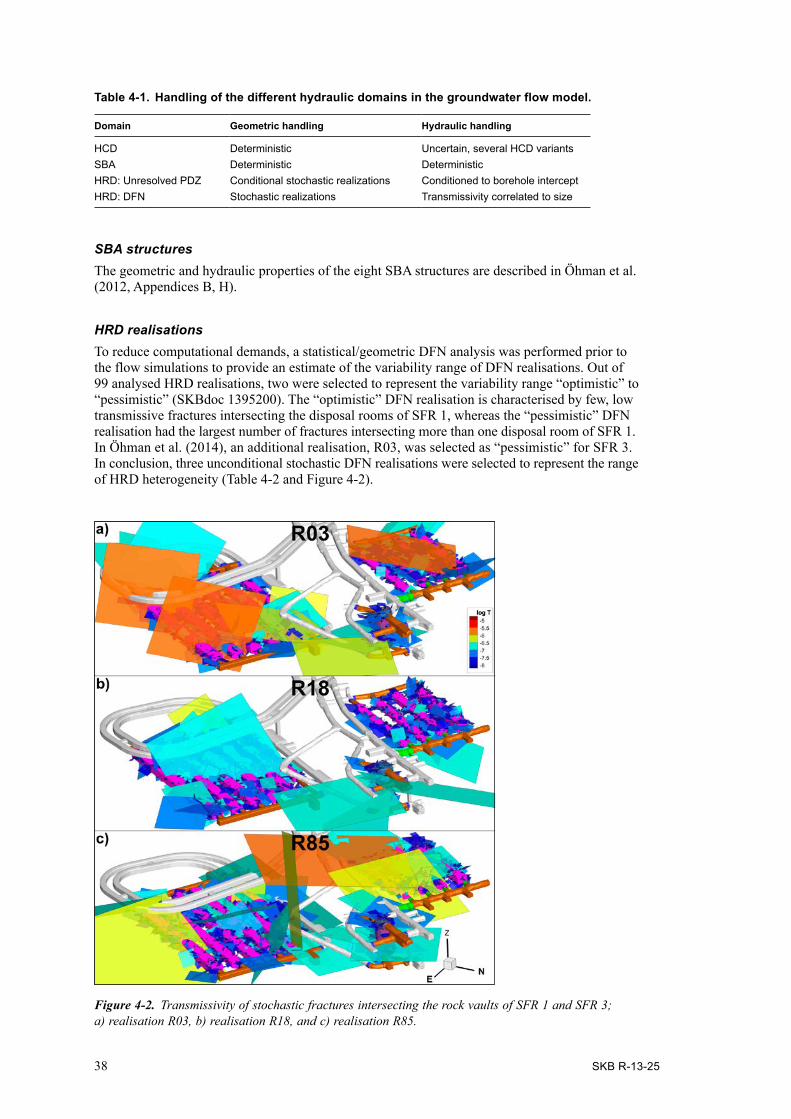
38 SKB R-13-25

Table 4-1. Handling of the different hydraulic domains in the groundwater flow model.

Domain Geometric handling Hydraulic handling

HCD Deterministic Uncertain, several HCD variantsSBA Deterministic DeterministicHRD: Unresolved PDZ Conditional stochastic realizations Conditioned to borehole interceptHRD: DFN Stochastic realizations Transmissivity correlated to size

SBA structuresThe geometric and hydraulic properties of the eight SBA structures are described in Öhman et al. (2012, Appendices B, H).

HRD realisations To reduce computational demands, a statistical/geometric DFN analysis was performed prior to the flow simulations to provide an estimate of the variability range of DFN realisations. Out of 99 analysed HRD realisations, two were selected to represent the variability range “optimistic” to “pessimistic” (SKBdoc 1395200). The “optimistic” DFN realisation is characterised by few, low transmissive fractures intersecting the disposal rooms of SFR 1, whereas the “pessimistic” DFN realisation had the largest number of fractures intersecting more than one disposal room of SFR 1. In Öhman et al. (2014), an additional realisation, R03, was selected as “pessimistic” for SFR 3. In conclusion, three unconditional stochastic DFN realisations were selected to represent the range of HRD heterogeneity (Table 4-2 and Figure 4-2).

Figure 4-2. Transmissivity of stochastic fractures intersecting the rock vaults of SFR 1 and SFR 3; a) realisation R03, b) realisation R18, and c) realisation R85.

SKB R-13-25 39

Table 4-2. Selected HRD realisations.

Variant Description

R03 Pessimistic for SFR 3 (4BLA, 5BLA and 2BMA), but also for 1BMAR18 Optimistic realisation for existing SFR 1 (few large fractures connecting rock vaults in existing SFR 1)R85 Pessimistic realisation for existing SFR 1 (large fractures connecting rock vaults in existing SFR 1)

HCD variantsThe HCD geometry is based on two data sources: 1) The geological model v.1.0 (Curtis et al. 2011), and 2) Six extended HCDs (NNW3113, NNW0999, NS3154, NNE3266, NNE3265, and NNE3264) that, based on lineament data, extend outside the SFR Regional domain (see recommendations in Öhman et al. (2013), Section 3.2). These HCDs are not defined in the geological model v.1.0 outside the SFR Regional domain. The reason for extending the six HCDs is to eliminate the risk of par-ticle-tracking artefacts that are related to model-boundary terminations of zones. The uncertainties in HCD geometry are less than the uncertainties in hydraulic parameterisation. Different hydraulic properties are therefore tested, while the geometry is fixed. These comprise the following.

Transmissivity variability: HCDs are modelled as either homogeneous (labelled Base Case and HOM in Table 4-3) or heterogeneous (HCD hydraulic realisations R01 and R07, both selected as “pessimistic” in SKBdoc 1395215, based on preceding simulations in SKBdoc 1395214.

• Borehole conditioning: Borehole data in the elevation interval of the planned SFR 3 indicate low transmissivity of ZFMWNW0835 and ZFMENE3115 (Figure 4-3a). The confidence in bore-hole conditioning is unclear, i.e. how far can the observed low transmissivity data be extrapolated without being overly optimistic regarding the restriction on groundwater flow this implies?

• Depth trend: Two alternatives are compared: 1) assuming the established HCD depth trend in SDM-Site Forsmark:

T (z) = T (0) 10 z/k (Eq. 4-1)

where T (z) is the flow model deformation zone transmissivity, z is the elevation (positive upwards), T (0) is the expected value of the transmissivity of the deformation zone at zero eleva-tion, and k is the depth interval that gives an order of magnitude decrease of the transmissivity; the (transmissivity parameterisation is presented in SKB 2013, Appendix 6) versus,

2) no depth trend (transmissivity parameterisation presented in Öhman et al. (2014).

• Anisotropic Southern boundary belt (SBB): In SDM-Site Forsmark, the Singö deformation zone was hypothesised as anisotropic (less transmissive across the structure). This hypothesis is partially tested in one of the 17 bedrock cases (referred to as BASE_CASE2)

Implementation of selected HCD variantsThe four concepts can be combined to form a number of HCD variants; ten of these parameterisation variants (Table 4-3) are selected for the sensitivity analysis.

Table 4-3. Notation of HCD variants.

HCD variant Conditioning Depth trend Transmissivity variability

BASE_CASE1 Yes Yes HomogeneousBASE_CASE2 Yes Yes Homogeneous, Anisotropic SBBnc_DEP_HOM No Yes Homogeneousnc_NoD_HOM No No HomogeneousCD_DEP_R01 Yes Yes Heterogeneous, R01nc_DEP_R01 No Yes Heterogeneous, R01CD_DEP_R07 Yes Yes Heterogeneous, R07nc_DEP_R07 No Yes Heterogeneous, R07nc_NoD_R01 No No Heterogeneous, R01nc_NoD_R07 No No Heterogeneous, R07

40 SKB R-13-25

Two zones have been identified as particularly significant for SFR 3 (ZFMWNW0835 and ZFMENE3115) because they intersect some of the rock vaults. As a demonstration of the HCD parameterisation variants, the parameter ranges of these two zones are shown in context of SFR 3 and field data (Figure 4-3 and Figure 4-4).

4.3.3 Bedrock outside SFR Regional domainThe bedrock description outside the SFR Regional domain is taken from SR-Site/SDM-Site Forsmark (see Öhman et al. 2014) and kept constant in all model setups.

Figure 4-3. Studied variants of heterogeneous HCD models of the two key zones for the planned exten-sion. The spatial variability is represented by a tessellation of ca.50 m. The depth-dependent variants are: a) “nc_DEP_R01”: non-conditioned realisation R01, b) “nc_DEP_R07”: non-conditioned realisation R01 R07, c) “nc_DEP_R01”: conditioned realisation R01, and d)“nc_DEP_R07”: conditioned realisationR07. The non-conditioned realisations of c) and d) without depth dependence are shown in e) and f,) respectively,.

SKB R-13-25 41

Figure 4-4. Heterogeneous HCD variants of the two key zones for the planned extension (the tessellation is c. 50 m); the depth-dependent variants are: a) non-conditioned realisation R01, b) non-conditioned realisations R01 and R07, c) conditioned realisation R01,and d) conditioned realisations R01 and R07. The corresponding non-conditioned variants without depth dependence are shown in e) and f), respectively.

4.3.4 Model variants in SR-PSUThis section summarizes the different model variants used in SR-PSU, Table 4-1 lists the different model components. The combined components of uncertainty/heterogeneity in the bedrock proper-ties are analysed in terms of a sensitivity analysis, where model performance is evaluated for a selec-tion of 17 bedrock cases (Table 4-4) and 6 stages of shoreline displacement. These bedrock cases were chosen to capture the uncertainty/variability in the bedrock parameterisation. Hence, they can be assumed to demonstrate the variation of flow through the disposal rooms.

42 SKB R-13-25

Table 4-4. Bedrock cases studied in the sensitivity analysis.

No. LabelHCD

HRDConditioning Depth trend Variability

1 BASE_CASE1_DFN_R85

Yes

Yes

HomogeneousR85

2 BASE_CASE1_DFN_R18 R18

3 BASE_CASE2_DFN_R85 Anisotropic SBB R85

4 nc_DEP_HOM_DFN_R03

No Homogeneous

R03

5 nc_DEP_HOM_DFN_R85R85

6 nc_NoD_HOM_DFN_R85 No

7 CD_DEP_R01_DFN_R85 Yes

Yes

Heterogeneous, R01R85

8 nc_DEP_R01_DFN_R85No

9 nc_DEP_R01_DFN_R18 R18

10 CD_DEP_R07_DFN_R85 Yes

Heterogeneous, R07R85

11 nc_DEP_R07_DFN_R85

No

12 nc_DEP_R07_DFN_R18 R18

13 nc_NoD_R01_DFN_R03

No

Heterogeneous, R01

R03

14 nc_NoD_R01_DFN_R85 R85

15 nc_NoD_R01_DFN_R18 R18

16 nc_NoD_R07_DFN_R03Heterogeneous, R07

R03

17 nc_NoD_R07_DFN_R85 R85

4.4 Boundary conditionsAs mentioned in Section 3.3.2 the flow model domain follows present and future topographical water divides. The vertical sides and the bottom are therefore assigned no-flow boundary conditions, which imply that recharge and discharge are completely governed by climate-related processes pre-vailing on the top surface.

4.4.1 Top boundaryA hybrid approach is used in the flow model (Öhman et al. 2014) to mitigate the problem of flooding (excess heads), where the two boundary-condition types “flux” and “fixed head” are mixed in a pre-ceding “Recharge phase” to simulate a realistic head distribution for the model top boundary (allow-ing unsaturated areas, but not excess head). The top-boundary head is then applied as a fixed-head boundary condition in subsequent steady state simulations, in order to establish a highly convergent flow field.

4.4.2 Lakes and riversLakes are used as prescribed head-boundary conditions in the flow model (Öhman et al. 2014). More precisely, “Lake cells” are defined and refined in the computational grid by means of so-called “DarcyTools objects”. The prescribed-head values for lakes are taken from the modelled lake thresh-olds in RLDM. The number of lakes, as well as the spatial extent of individual lakes, varies over time. Lake data are also used as fixed points in defining prescribed head values along riverbeds.

Rivers are also treated as prescribed head-boundary conditions in the flow model. Unlike the lakes, the riverbed head varies along the trajectory of a modelled river, which requires a somewhat differ-ent modelling procedure. Similar to implementation of lakes, so-called “DarcyTools objects” are used to define “river cells” in the computational grid. Riverbed head is not provided in RLDM data, but is estimated according to principles described in Öhman et al. (2014).

SKB R-13-25 43

4.5 Results from the modelling of temperate climate conditionsBelow, performance measures from the modelling of temperate climate conditions are shown for the six time slices shown in Figure 3-10. Table 4-5 explains the contents shown in Figure 4-5 through Figure 4-23.

To comprehend the information provided in Figure 4-5 through Figure 4-23 the following is noted.

• All bedrock cases were studied at steady-state flow conditions, which mean that the particle tracking was made for a fixed velocity field.

• The cross flow value of the flow through a rock vault (Q in m3/s) was calculated by a summation of the local flow rates, Qi, flowing through the grid cell faces that connect to the rock vault. Qi was calculated by multiplying Darcy flux by the grid cell area facing the rock vault.

• 1,000,000 particles were traced downstream starting at the rock vaults and stopping at the bed-rock-regolith interface. (The discharge locations at this interface are called exit locations below.) Cumulative values of the flow-related transport resistance in rock (Fr in y/m), advective travel time in rock (tw,r in y), and path length in rock (Lr in m) were calculated for each particle.

• The cumulative flow-related transport resistance was calculated by a summation of the local flow-related transport resistances, Fi, inferred from each grid cell that was passed through during the particle tracking. Fi was calculated by multiplying the grid cell flow-wetted fracture surface area per unit volume of water by the local advective travel time.

• The cumulative value of the advective travel time in the bedrock (tw,r in y) was calculated by a summation of the local advective travel times, tw,i, spent in each grid cell during the particle tracking. tw,i was calculated by dividing the local path length in the cell by the advective trans-port velocity. The latter was calculated by dividing the Darcy flux in the cell by the grid cell kinematic (fracture) porosity.

• The cumulative value of the path length in the bedrock (Lr in m) was calculated by a summation of the discrete particle steps, Li, calculated as the distance between cell-wall centre points of each grid cell passed during the particle tracking.

Table 4-5. Overview of information shown in Figure 4-5 through Figure 4-23.

Figure Facility Bedrock case (cf. Table 4-5)

Parameter Type of plot

Figure 4-5 SFR 1 1-17 Q Box and WhiskerFigure 4-6 SFR 3 1-17 Q Box and WhiskerFigure 4-7 SFR 1, SFR 3 1-17 Median Q Q = Q(t)Figure 4-8 SFR 1, SFR 3 1,15,11 Median Fr Fr = Fr (t)Figure 4-9 SFR 1, SFR 3 1,15,11 Median tw,r tw = tw(t)Figure 4-10 SFR 1, SFR 3 1,15,11 Median Lr Lr = Lr(t)Figure 4-11 SFR 1, SFR 3 1 Exit locations Map 2000, 2500, 3000 ADFigure 4-12 SFR 1, SFR 3 1 Exit locations Map 3500, 5000, 9000 ADFigure 4-13 SFR 1, SFR 3 1 Recharge locations 3D view of biosphere object 157:2 at 5000 ADFigure 4-14 SFR 1, SFR 3 1 Recharge locations Map of biosphere object 157:2 at 5000 ADFigure 4-15 SFR 1, SFR 3 1 Fr Cumulative distributionFigure 4-16 SFR 1, SFR 3 15 Fr Cumulative distributionFigure 4-17 SFR 1, SFR 3 11 Fr Cumulative distributionFigure 4-18 SFR 1, SFR 3 1 tw,r Cumulative distributionFigure 4-19 SFR 1, SFR 3 15 tw,r Cumulative distributionFigure 4-20 SFR 1, SFR 3 11 tw,r Cumulative distributionFigure 4-21 SFR 1, SFR 3 1 Lr Cumulative distributionFigure 4-22 SFR 1, SFR 3 15 Lr Cumulative distributionFigure 4-23 SFR 1, SFR 3 11 Lr Cumulative distribution

44 SKB R-13-25

The information shown in Figure 4-5 through Figure 4-10 can be summarised as follows.

• The median values of Q and Lr both increase in accordance with the shoreline retreat up to about 5000 AD. Thereafter, the driving force associated with the Baltic Sea becomes less important than the driving force associated to local topography. Hence, “constant median values” of the studied parameters Fr and tw,r are obtained after about 5000 AD. The box and whisker plots show an increasing spread with time as the discharge takes place at different topo graphic locations.

The information shown in Figure 4-11 through Figure 4-14 can be summarised as follows.

• The exit locations of particles starting in SFR 1 are more or less independent of the shoreline displacement. The majority of the exit locations end up adjacent to an area located in the vicinity of the junction between two steeply dipping deformation zones. The area has been denoted “bio-sphere object 157_2”, see Figure 4-11. In contrast, the exit locations of particles starting in SFR 3 vary as the shoreline retreats up to about 5000 AD. Thereafter, the discharge conditions are asso-ciated with undulations in the surface topography.

• A total of about 4% of the discharge to biosphere object 157_2 passes through the rock vaults of SFR 1 and SFR 3.

The information shown in Figure 4-15 through Figure 4-23 can be summarised as follows.

• At 2000 AD the distributions of Fr and tw,r for particles starting in SFR 3 have similar or lower median values than those for the particles starting in SFR 1 regardless of bedrock case (discussed in Öhman et al. 2014, Appendix B). At future time slices, the situation is the opposite due to the shoreline displacement (see below).

• Regarding Lr, the particles starting in SFR 1 always have a lower median value than the parti-cles starting in SFR 3 regardless of bedrock case and time slice. This is because SFR 3 is located deeper than SFR 1.

4.5.1 Cross flowFigure 4-5 and Figure 4-6 show that the median values of the cross flow Q increase in accordance with the shoreline retreat up to about 5000 AD. Thereafter, the driving force associated with the Baltic Sea becomes less important than the driving force associated to local topography. The cross flow s at 2000 AD, 3000 AD, and 5000 AD are tabulated in Table 4-6 and Table 4-7.

Table 4-6. Tabulation of the cross flows (m3/year) shown in Figure 4-5.

Median 1BTF 2BTF 1BLA 1BMA Silo

2000 0.07 0.07 0.12 0.09 0.00163000 20.51 22.35 63.64 57.86 0.325000 44.60 47.81 130.96 112.56 1.11

Min 1BTF 2BTF 1BLA 1BMA Silo

2000 0.03 0.04 0.04 0.04 0.00083000 12.10 13.83 18.72 38.82 0.145000 25.35 26.46 35.40 75.74 0.66

Max 1BTF 2BTF 1BLA 1BMA Silo

2000 0.17 0.26 0.53 0.68 0.00553000 24.46 58.38 157.79 146.74 0.445000 54.17 113.08 305.58 281.39 1.61

SKB R-13-25 45

Figure 4-5. Box-and-whisker plots of simulated disposal room cross flow rates in the sensitivity study of 17 bedrock cases (Table 4-4). The progress over time is shown for six time slices. Individual rock vaults of SFR 1 are compared in a) to e). To resolve the low early cross flow through the Silo, both linear e) and logarithmic scales f) are compared.

00.

050.

1

2000 AD 2500 AD 3000 AD 3500 AD 5000 AD 9000 AD

Tunn

el fl

ow, Q

(L/m

in)

a) 1BTF0

0.05

0.1

0.15

0.2

2000 AD 2500 AD 3000 AD 3500 AD 5000 AD 9000 AD

Tunn

el fl

ow, Q

(L/m

in)

b) 2BTF

00.

001

0.00

20.

003

2000 AD 2500 AD 3000 AD 3500 AD 5000 AD 9000 AD

Tunn

el fl

ow, Q

(L/m

in)

e) Silo

00.

10.

20.

30.

40.

50.

6

2000 AD 2500 AD 3000 AD 3500 AD 5000 AD 9000 AD

Tunn

el fl

ow, Q

(L/m

in)

d) 1BMA

00.

10.

20.

30.

40.

50.

6

2000 AD 2500 AD 3000 AD 3500 AD 5000 AD 9000 AD

Tunn

el fl

ow, Q

(L/m

in)

c) 1BLA

0.00

0001

0.00

001

0.00

010.

001

2000 AD 2500 AD 3000 AD 3500 AD 5000 AD 9000 AD

Tunn

el fl

ow, Q

(L/m

in)

f) Silo

SFR 1

Table 4-7. Tabulation of the cross flows (m3/year) shown in Figure 4-6.

Median 1BRT 2BLA 3BLA 4BLA 5BLA 2BMA 1BRT

2000 0.21 0.17 0.14 0.14 0.20 0.43 0.213000 15.67 22.67 21.77 22.46 22.88 46.76 15.675000 27.93 42.92 33.98 34.19 34.13 66.27 27.93

Min 1BRT 2BLA 3BLA 4BLA 5BLA 2BMA 1BRT

2000 0.10 0.10 0.10 0.08 0.10 0.14 0.103000 8.15 12.20 14.94 16.67 15.73 27.40 8.155000 15.04 25.51 23.46 25.77 25.04 34.24 15.04

Max 1BRT 2BLA 3BLA 4BLA 5BLA 2BMA 1BRT

2000 0.38 0.35 0.22 0.29 0.29 0.77 0.383000 28.77 37.55 27.35 42.76 65.22 93.09 28.775000 50.23 64.69 41.87 76.79 111.50 134.12 50.23

46 SKB R-13-25

Comparisons with cross flow results for SFR 1 reported in SAR-08The transformation of pressure measurements made in boreholes drilled from floating platforms prior to the construction of SFR 1 indicated that the groundwater levels in the shallow bedrock in the SFR area could be higher than mean sea water level (so called ‘excess head’). Different hypotheses to explain the excess head have been discussed in Carlsson et al. (1987) who concluded, however, that the existence of an ‘excess head’ is highly uncertain due to the poor measurement and evaluation techniques used, and that the reported excess head was too high or probably missing.

Notwithstanding, in the previous safety assessment (SAR-08) an attempt was made to represent the excess head in the flow model at 2000 AD (Holmén and Stigsson 2001). It was stated that “... the uncer-tainty in the measured and interpreted values of excess head, will only have a large influence in predicted flow, for the time period between 2000 AD and 3000 AD”. In SR-PSU, no attempt has been made to represent the excess head in the analyses based on the conclusions of Carlsson et al. (1987). Therefore, the results presented in Holmén and Stigsson (2001) indicates higher flow through the rock vaults at 2000 AD than in SR-PSU. However, the medians flows at 3000 AD are almost identical, see Table 4-8.

00.

050.

1

2000 AD 2500 AD 3000 AD 3500 AD 5000 AD 9000 AD

Tunn

el fl

ow, Q

(L/m

in)

a) 1BRT

00.

050.

1

2000 AD 2500 AD 3000 AD 3500 AD 5000 AD 9000 AD

Tunn

el fl

ow, Q

(L/m

in)

b) 2BLA0

0.01

0.02

0.03

0.04

0.05

0.06

0.07

0.08

2000 AD 2500 AD 3000 AD 3500 AD 5000 AD 9000 AD

Tunn

el fl

ow, Q

(L/m

in)

c) 3BLA

00.

050.

10.

15

2000 AD 2500 AD 3000 AD 3500 AD 5000 AD 9000 AD

Tunn

el fl

ow, Q

(L/m

in)

d) 4BLA

00.

050.

10.

150.

2

2000 AD 2500 AD 3000 AD 3500 AD 5000 AD 9000 AD

Tunn

el fl

ow, Q

(L/m

in)

e) 5BLA

00.

10.

2

2000 AD 2500 AD 3000 AD 3500 AD 5000 AD 9000 AD

Tunn

el fl

ow, Q

(L/m

in)

f) 2BMA

SFR 3

Figure 4-6. Box-and-whisker plots of simulated disposal room cross flow in the sensitivity study of 17 bedrock cases (Table 4-4). The progress over time is shown for six time slices. Individual rock vaults of SFR 3 are compared in a) to f).

SKB R-13-25 47

Table 4-8. Comparisons with cross flow results for SFR 1 reported in SAR-08 at 2000 AD, 3000 AD, and 5000 AD (m3/year).

2000 AD 3000 AD 5000 ADRock vault SAR-08 SR-PSU SAR-08 SR-PSU SAR-08 SR-PSU

1BTF 13 0.07 38 20.51 43 44.602BTF 12 0.07 33 22.35 41 47.811BLA 15 0.12 42 63.64 61 130.961BMA 4.8 0.09 50 57.86 65 112.56Silo 0.6 0.0016 2.3 0.32 3.9 1.11Total 45.4 0.35 165.3 164.68 213.9 337.04

4.5.2 Median values of Q, Fr, tw,r, and Lr

Figure 4-7 through Figure 4-10 show that the median values of Q and Lr both increase in accordance with the shoreline retreat up to about 5000 AD. Thereafter, the driving force imposed by the down-stream condition associated with the Baltic Sea becomes less important relative to topographically driven flow. Hence, “constant median values” of the studied parameters Fr and tw,r are obtained after about 5000 AD. The box and whisker plots show an increasing spread with time as the discharge takes place at different topographic locations. Table 4-9 show median, minimum and maximum values of Q, Fr, tw,r and Lr at three characteristic time slices.

Figure 4-7. Median values of the cross flows according to rock vault: a) in SFR 1 and b) in SFR 3. The results are taken over all bedrock cases as indicated by the range of the bars.

Figure 4-8. Median values of the flow-related transport resistances (Fr) according to rock vault and time: a) in SFR 1 and b) in SFR 3. The results are taken over three bedrock cases (1, 15, and 11) as indicated by the range of the bars.

1E+3

1E+4

1E+5

1E+6

1E+7

2000 3000 4000 5000 6000 7000 8000 9000

F r (y

/m)

1BTF 2BTF

1BLA 1BMA

Silo

a)

1E+3

1E+4

1E+5

1E+6

1E+7

2000 3000 4000 5000 6000 7000 8000 9000

F r (y

/m)

1BRT 2BLA

3BLA 4BLA

5BLA 2BMA

b)

1E-6

1E-5

1E-4

1E-3

1E-2

1E-1

2000 3000 4000 5000 6000 7000 8000 9000

Med

ian

cros

s flo

w (L

/min

)

1BTF 2BTF

1BLA 1BMA

Silo

a)

1E-6

1E-5

1E-4

1E-3

1E-2

1E-1

2000 3000 4000 5000 6000 7000 8000 9000

Med

ian

cros

s flo

w (L

/min

)

1BRT 2BLA

3BLA 4BLA

5BLA 2BMA

b)

48 SKB R-13-25

Table 4-9. Compilation of performance measures for 1BMA at 2000 AD, 3000 AD, and 5000 AD.

Parmeter 2000 AD median

2000 ADmin

2000 ADmax

3000 AD median

3000 ADmin

3000 ADmax

5000 ADmedian

5000 ADmin

5000 ADmax

Q (L/min) 1.8E–04 7.6E–05 1.3E–03 1.1E–01 7.4E–02 2.8E–01 2.1E–01 1.4E–01 5.4E–01Fr (y/m) 3.8E+06 2.0E+06 6.2E+06 1.1E+04 4.4E+03 1.3E+04 4.9E+03 3.9E+03 7.8E+03tw,r (y) 640 489 916 1.6 1.0 1.6 0.8 0.8 0.9Lr (m) 92 89 133 243 240 251 436 372 498

Table 4-10. Compilation of performance measures for the Silo at 2000 AD, 3000 AD, and 5000 AD.

Parmeter 2000 AD median

2000 ADmin

2000 ADmax

3000 AD median

3000 ADmin

3000 ADmax

5000 ADmedian

5000 ADmin

5000 ADmax

Q (L/min) 3.1E–06 1.5E–06 1.0E–05 6.1E–04 2.7E–04 8.4E–04 2.1E–03 1.3E–03 3.1E–03Fr (y/m) 1.6E+07 4.2E+06 2.1E+07 8.9E+04 8.2E+04 1.1E+05 2.3E+04 2.2E+04 3.1E+04tw,r (y) 2,096 812 2,941 9.4 6.3 9.5 2.1 1.5 2.4Lr (m) 148 137 149 320 284 346 480 439 504

Table 4-11. Compilation of performance measures for 2BMA at 2000 AD, 3000 AD, and 5000 AD.

Parmeter 2000 AD median

2000 ADmin

2000 ADmax

3000 AD median

3000 ADmin

3000 ADmax

5000 ADmedian

5000 ADmin

5000 ADmax

Q (L/min) 8.3E–04 2.6E–04 1.5E–03 8.9E–02 5.2E–02 1.8E–01 1.3E–01 6.5E–02 2.6E–01Fr (y/m) 2.9E+06 6.3E+05 4.8E+06 5.8E+04 5.4E+04 6.4E+04 5.3E+04 4.8E+04 5.5E+04tw,r (y) 386 146 555 5.7 4.8 6.6 4.4 3.7 4.7Lr (m) 209 177 232 597 507 657 844 822 988

Figure 4-9. Median values of the advective travel times (tw,r)according to rock vault and time: a) in SFR 1 and b) in SFR 3. The results are taken over three bedrock cases (1, 15, and 11) as indicated by the range of the bars.

Figure 4-10. Median values of the path lengths (Lr) according to rock vault and time; a) in SFR 1 and b) in SFR 3. The results are taken over three bedrock cases (1, 15, and 11) as indicated by the range of the bars.

0.1

1

10

100

1000

2000 3000 4000 5000 6000 7000 8000 9000

t w,r

(y)

1BTF 2BTF

1BLA 1BMA

Silo

a)

0.1

1

10

100

1000

2000 3000 4000 5000 6000 7000 8000 9000

t w,r

(y)

1BRT 2BLA

3BLA 4BLA

5BLA 2BMA

b)

0

200

400

600

800

1000

2000 3000 4000 5000 6000 7000 8000 9000

L r (m

)

1BTF 2BTF

1BLA 1BMA

Silo

a)

0

200

400

600

800

1000

2000 3000 4000 5000 6000 7000 8000 9000

L r (m

)

1BRT 2BLA

3BLA 4BLA

5BLA 2BMA

b)

SKB R-13-25 49

4.5.3 Exit locationsExit locations for flow across rock vaults were simulated by means of forward particle tracking. The spatial distribution of these locations was quantified in terms of areal density, number of particles/m2, based on 1,000,000 particles released uniformly within each disposal room of SFR 1 and SFR 3, respectively. The starting points of trajectories were defined at the tunnel-wall passage, and the ter-mination locations were defined at the bedrock/regolith interface passage.

The patterns in exit locations of SFR 1 and SFR 3 were compared over time, in terms of the six selected time slices (Figure 4-11 and Figure 4-12).

Figure 4-11. Exit locations for particles starting in the SFR 1 rock vaults (pink shade; left) and in the SFR 3 rock vaults (pink shade; right), Bedrock case 1, time slices 2000 to 3000 AD.

50 SKB R-13-25

Figure 4-12. Exit locations for particles starting in the SFR 1 rock vaults (pink shade; left) and in the SFR 3 rock vaults (pink shade; right), Bedrock case 1, time slices 3500 to 9000 AD.

SKB R-13-25 51

In the present report only the exit locations for Bedrock case 1 are shown, however in TD10 (SKBdoc 1395215) it was shown that the different Bedrock cases have similar exit locations. Two specific characteristics should be noted:

• Shoreline displacement successively forces the exit locations further away from the release points. Before the time slice 3500 AD, exit locations are essentially adjacent to the shoreline. The flow regime changes from being mainly upward-directed during early time slices to being more hori-zontal at later time slices. (As shown in Section 4.5.4 a large number of particles discharges in bio-sphere object 157_2.)

• The density of exit locations is strongly correlated to ground intercepts of deformation zones (most likely also transmissive stochastic DFN fractures). The dominant discharge path for SFR 1 is ZFMNNW1209 (Zone 6) during time slices 2000 to 2500 AD, after which ZFMNNE0869 and ZFMNW0805A/B dominate during time slices 3000 to 3500 AD. The pattern of exit locations from SFR 1 appears stationary between time slices 5000 and 9000 AD and in essence, all particles discharge to biosphere object 157_2 (see below). During early stages, SFR 3 has exit locations both north and south of the SFR pier. As the horizontal component in the flow regime successively grows, the exit locations are driven north, towards ZFMNW0805A/B and ZFMNS3154. Most particles discharge into biosphere object 157_2, although owing to its deeper location, a lesser number of particles discharge into biosphere objects related to biosphere object 116.

4.5.4 Discharge to biosphere object 157_2The area where biosphere object 157_2 is situated (Figure 4-13) is an important discharge area for the SR-PSU project. At later stages of shoreline displacement, beginning at about 3500 AD, a high density of particle-exit locations is obtained in object 157_2. There are several reasons for this.

1) Geology: Groundwater flows from SFR (i.e. downstream flow paths) are more or less enclosed by three deformation zones: the steeply dipping zones NNE0869 and NW0805A/B (Figure 4-13), and the gently dipping zone ZFM871 located just below the existing SFR facility. The junction between these deformation zones occurs underneath biosphere object 157_2.

2) Location and topography: Biosphere object 157_2 is a local topographical depression just north of SFR, which according to the topographical gradient is downstream of SFR.

3) Sediment coverage: the thickness of low-conductive sediment layers is thin north of the pier.

It is therefore of interest to perform backward-particle tracking, to determine the source of discharg-ing groundwater, i.e. the amount of this groundwater passing through the SFR facility. 1,000,000 par-ti cles were released at the bedrock surface inside biosphere object 157_2. The reversed (backward) flow trajectories contoured by head are showed in Figure 4-13 and recharge locations in Figure 4-14. About 4% of the discharge to biosphere object 157_2 passes through the disposal facilities SFR 1 or SFR 3 at 5000 AD (Table 4-12).

Table 4-12. Fraction of recharge crossing rock vaults, 5000 AD.

Disposal facility Recharge fraction

1BTF 0.29%2BTF 0.36%1BLA 1.25%1BMA 0.66%Silo 0.02%2BLA 0.45%3BLA 0.26%4BLA 0.15%5BLA 0.12%2BMA 0.17%1BRT 0.34%Total 4.06%

52 SKB R-13-25

Figure 4-13. Backward particle-tracking from biosphere object ID 157_2, bedrock case 1, 5000 AD; a) particle-release points contoured by elevation, and b) backward flow trajectories contoured by head (m), SFR tunnels shaded by back-fill material (see Figure 3-7), and ground intercepts with deformation zones grey-shaded.

Figure 4-14. Recharge locations for biosphere object ID 157_2, Bedrock case 1, 5000 AD; a) particle-release points for backward particle-tracking (pink) and b) areal density of recharge locations. 1,000,000 particles released at bedrock surface. A few recharge locations begin in the Forsmark inland area (not shown).

SKB R-13-25 53

4.5.5 Flow-related transport resistanceFigure 4-15 through Figure 4-17 show the cumulative distributions of Fr for three bedrock cases presented in Table 4-4, No 1, No 15, and No 11. At 2000 AD, the cumulative distributions of Fr for particles starting in SFR 1 and SFR 3 are closer to each other than at future time slices. At future time slices, particles starting in SFR 3 have typically greater median values owing to its deeper loca-tion. The differences between the three bedrock cases are fairly small in terms of median values. The greatest spread is observed for bedrock case no. 11. Table 4-13 through Table 4-15 show the medi-ans, 5% percentiles, and 95% percentiles of Fr for SFR 1 and SFR 3 at three time slices.

Bedrock case 1 [BASE_CASE1_DFN_R85]

Table 4-13. Bedrock case 1: Compilation of medians, 5% percentiles, and 95% percentiles of Fr in (y/m) at three time slices 2000 AD, 3000 AD, and 5000 AD for SFR 1 and SFR 3.

Source 2000 AD median

2000 AD5%

2000 AD95%

3000 AD median

3000 AD5%

3000 AD95%

5000 ADmedian

5000 AD5%

5000 AD95%

SFR 1 7.1E+06 9.4E+05 3.8E+07 3.7E+04 6.0E+03 2.2E+05 9.5E+03 3.1E+03 6.0E+04SFR 3 6.5E+06 1.3E+06 2.6E+07 7.8E+04 1.6E+04 4.4E+05 5.0E+04 1.2E+04 3.5E+05

Figure 4-15. Evolution of the distribution of Fr with time for bedrock case 1 [BASE_CASE1_DFN_R85].

00.10.20.30.40.50.60.70.80.9

1

1E+3 1E+4 1E+5 1E+51E+6 1E+7 1E+8

Frac

�on

(-)

Frac

�on

(-)

Frac

�on

(-)

Frac

�on

(-)

Frac

�on

(-)

Frac

�on

(-)

F-quo�ent (yr/m) F-quo�ent (yr/m)

F-quo�ent (yr/m)F-quo�ent (yr/m)

F-quo�ent (yr/m)F-quo�ent (yr/m)

SFR1SFR3

a) 2000 AD

00.10.20.30.40.50.60.70.80.9

1

1E+3 1E+4 1E+6 1E+7 1E+8

SFR1SFR3

b) 2500 AD

00.10.20.30.40.50.60.70.80.9

1

1E+3 1E+4 1E+5 1E+6 1E+7 1E+8

SFR1SFR3

c) 3000 AD

00.10.20.30.40.50.60.70.80.9

1

1E+3 1E+4 1E+5 1E+6 1E+7 1E+8

SFR1SFR3

d) 3500 AD

00.10.20.30.40.50.60.70.80.9

1

1E+3 1E+4 1E+5 1E+6 1E+7 1E+8

SFR1SFR3

e) 5000 AD

00.10.20.30.40.50.60.70.80.9

1

1E+3 1E+4 1E+5 1E+6 1E+7 1E+8

SFR1SFR3

f) 9000 AD

54 SKB R-13-25

Bedrock case 15 [nc_NoD_R01_DFN_R18]

Table 4-14. Bedrock case 15: Compilation of medians, 5% percentiles, and 95% percentiles of Fr in (y/m) at three time slices 2000 AD, 3000 AD, and 5000 AD for SFR 1 and SFR 3.

Source 2000 AD median

2000 AD5%

2000 AD95%

3000 AD median

3000 AD5%

3000 AD95%

5000 ADmedian

5000 AD5%

5000 AD95%

SFR 1 2.6E+06 9.6E+05 1.1E+07 6.0E+04 6.4E+03 3.6E+05 2.3E+04 3.3E+03 1.4E+05SFR 3 4.5E+06 1.4E+06 1.9E+07 7.9E+04 1.8E+04 6.0E+05 6.0E+04 1.4E+04 3.1E+05

Figure 4-16. Evolution of the distribution of Fr with time for bedrock case 15 [nc_NoD_R01_DFN_R18].

00.10.20.30.40.50.60.70.80.9

1

1E+3 1E+4 1E+5 1E+6 1E+7 1E+8

Frac

�on

(-)Fr

ac�o

n (-)

Frac

�on

(-)

Frac

�on

(-)Fr

ac�o

n (-)

Frac

�on

(-)

F-quo�ent (yr/m) F-quo�ent (yr/m)

F-quo�ent (yr/m) F-quo�ent (yr/m)

F-quo�ent (yr/m) F-quo�ent (yr/m)

SFR1SFR3

a) 2000 AD

00.10.20.30.40.50.60.70.80.9

1

1E+3 1E+4 1E+5 1E+6 1E+7 1E+8

SFR1SFR3

b) 2500 AD

00.10.20.30.40.50.60.70.80.9

1

1E+3 1E+4 1E+5 1E+6 1E+7 1E+8

SFR1SFR3

c) 3000 AD

00.10.20.30.40.50.60.70.80.9

1

1E+3 1E+4 1E+5 1E+6 1E+7 1E+8

SFR1SFR3

d) 3500 AD

00.10.20.30.40.50.60.70.80.9

1

1E+3 1E+4 1E+5 1E+6 1E+7 1E+8

SFR1SFR3

e) 5000 AD

00.10.20.30.40.50.60.70.80.9

1

1E+3 1E+4 1E+5 1E+6 1E+7 1E+8

SFR1SFR3

f) 9000 AD

SKB R-13-25 55

Bedrock case 11 [nc_DEP_R07_DFN_R85]

Table 4-15. Bedrock case 11: Compilation of medians, 5% percentiles, and 95% percentiles of Fr in (y/m) at three time slices 2000 AD, 3000 AD, and 5000 AD for SFR 1 and SFR 3.

Source 2000 AD median

2000 AD5%

2000 AD95%

3000 AD median

3000 AD5%

3000 AD95%

5000 ADmedian

5000 AD5%

5000 AD95%

SFR 1 6.0E+06 8.2E+05 3.2E+07 2.6E+04 2.2E+03 2.8E+05 1.2E+04 1.4E+03 1.0E+05SFR 3 4.0E+06 3.5E+05 2.6E+07 7.5E+04 1.2E+04 9.0E+05 4.6E+04 8.6E+03 6.8E+05

Figure 4-17. Evolution of the distribution of Fr with time for bedrock case 11 [nc_DEP_R07_DFN_R85].

00.10.20.30.40.50.60.70.80.9

1

1E+3 1E+4 1E+5 1E+6 1E+7 1E+8

Frac

�on

(-)

F-quo�ent (yr/m)

SFR1SFR3

a) 2000 AD

00.10.20.30.40.50.60.70.80.9

1

1E+3 1E+4 1E+5 1E+6 1E+7 1E+8Fr

ac�o

n (-)

F-quo�ent (yr/m)

SFR1SFR3

b) 2500 AD

00.10.20.30.40.50.60.70.80.9

1

1E+3 1E+4 1E+5 1E+6 1E+7 1E+8

Frac

�on

(-)

F-quo�ent (yr/m)

SFR1SFR3

c) 3000 AD

00.10.20.30.40.50.60.70.80.9

1

1E+3 1E+4 1E+5 1E+6 1E+7 1E+8

Frac

�on

(-)

F-quo�ent (yr/m)

SFR1SFR3

d) 3500 AD

00.10.20.30.40.50.60.70.80.9

1

1E+3 1E+4 1E+5 1E+6 1E+7 1E+8

Frac

�on

(-)

F-quo�ent (yr/m)

SFR1SFR3

e) 5000 AD

00.10.20.30.40.50.60.70.80.9

1

1E+3 1E+4 1E+5 1E+6 1E+7 1E+8

Frac

�on

(-)

F-quo�ent (yr/m)

SFR1SFR3

f) 9000 AD

56 SKB R-13-25

4.5.6 Advective travel timeFigure 4-18 through Figure 4-20 show the cumulative distributions of tw,r for three bedrock cases presented in Table 4-4, No 1, No 15, and No 11. At 2000 AD, the cumulative distributions of tw,r for particles starting in SFR 1 and SFR 3 are closer to each other than at future time slices. At future time slices, particles starting in SFR 3 have greater median values. The differences between the three bedrock cases are fairly small in terms of median values. The greatest spread is observed for bedrock case No 11. Table 4-16 through Table 4-18 show the medians, 5% percentiles, and 95% percentiles of tw,r for SFR 1 and SFR 3 at three time slices.

Bedrock case 1 [BASE_CASE1_DFN_R85]

Table 4-16. Bedrock case 1: Compilation of medians, 5% percentiles, and 95% percentiles of tw,r in (y) at three time slices 2000 AD, 3000 AD, and 5000 AD for SFR 1 and SFR 3.

Source 2000 AD median

2000 AD5%

2000 AD95%

3000 AD median

3000 AD5%

3000 AD95%

5000 ADmedian

5000 AD5%

5000 AD95%

SFR 1 1,070 192 5,270 4.5 0.9 21 1.3 0.6 4.6SFR 3 725 194 2,200 6.8 2.4 42 3.8 1.5 29

Figure 4-18. Evolution of the distribution of tw,r for bedrock case 1 [BASE_CASE1_DFN_R85].

00.10.20.30.40.50.60.70.80.9

1

0.1 1 10 100 1000 10000 100000

Frac

�on

(-)

Travel �me (yrs)

SFR1SFR3

a) 2000 AD

00.10.20.30.40.50.60.70.80.9

1

0.1 1 10 100 1000 10000 100000

Frac

�on

(-)

Travel �me (yrs)

SFR1SFR3

b) 2500 AD

00.10.20.30.40.50.60.70.80.9

1

0.1 1 10 100 1000 10000 100000

Frac

�on

(-)

Travel �me (yrs)

SFR1SFR3

c) 3000 AD

00.10.20.30.40.50.60.70.80.9

1

0.1 1 10 100 1000 10000 100000

Frac

�on

(-)

Travel �me (yrs)

SFR1SFR3

d) 3500 AD

00.10.20.30.40.50.60.70.80.9

1

0.1 1 10 100 1000 10000 100000

Frac

�on

(-)

Travel �me (yrs)

SFR1SFR3

e) 5000 AD

00.10.20.30.40.50.60.70.80.9

1

0.1 1 10 100 1000 10000 100000

Frac

�on

(-)

Travel �me (yrs)

SFR1SFR3

f) 9000 AD

SKB R-13-25 57

Bedrock case 15 [nc_NoD_R01_DFN_R18]

Table 4-17. Bedrock case 15: Compilation of medians, 5% percentiles, and 95% percentiles of tw,r in (y) at three time slices 2000 AD, 3000 AD, and 5000 AD for SFR 1 and SFR 3.

Source 2000 AD median

2000 AD5%

2000 AD95%

3000 AD median

3000 AD5%

3000 AD95%

5000 ADmedian

5000 AD5%

5000 AD95%

SFR 1 562 213 1,620 4.8 1.0 25 1.7 0.5 9.0SFR 3 491 202 1,530 6.8 2.7 76 5.1 1.6 32

Figure 4-19. Evolution of the distribution of tw,r for bedrock case 15 [nc_NoD_R01_DFN_R18].

00.10.20.30.40.50.60.70.80.9

1

0.1 1 10 100 1000 10000 100000

Frac

�on

(-)

Frac

�on

(-)

Frac

�on

(-)

Frac

�on

(-)

Frac

�on

(-)

Frac

�on

(-)Travel �me (yrs)

SFR1SFR3

a) 2000 AD

00.10.20.30.40.50.60.70.80.9

1

0.1 1 10 100 1000 10000 100000Travel �me (yrs)

SFR1SFR3

b) 2500 AD

00.10.20.30.40.50.60.70.80.9

1

0.1 1 10 100 1000 10000 100000Travel �me (yrs)

SFR1SFR3

c) 3000 AD

00.10.20.30.40.50.60.70.80.9

1

0.1 1 10 100 1000 10000 100000Travel �me (yrs)

SFR1SFR3

d) 3500 AD

00.10.20.30.40.50.60.70.80.9

1

0.1 1 10 100 1000 10000 100000Travel �me (yrs)

SFR1SFR3

e) 5000 AD

00.10.20.30.40.50.60.70.80.9

1

0.1 1 10 100 1000 10000 100000Travel �me (yrs)

SFR1SFR3

f) 9000 AD

58 SKB R-13-25

Bedrock case 11 [nc_DEP_R07_DFN_R85]

Table 4-18. Bedrock case 11: Compilation of medians, 5% percentiles, and 95% percentiles of tw,r in (y) at three characteristic time slices 2000 AD, 3000 AD, and 5000 AD for SFR 1 and SFR 3.

Source 2000 AD median

2000 AD5%

2000 AD95%

3000 AD median

3000 AD5%

3000 AD95%

5000 ADmedian

5000 AD5%

5000 AD95%

SFR 1 948 168 4,360 3.3 0.5 23 1.6 0.3 6.9SFR 3 547 87 2,090 7.0 2.2 98 3.9 1.3 71

Figure 4-20. Evolution of the distribution of tw,r for bedrock case 11 [nc_DEP_R07_DFN_R85].

Frac

�on

(-)

Frac

�on

(-)

Frac

�on

(-)

Frac

�on

(-)

Frac

�on

(-)

Frac

�on

(-)

00.10.20.30.40.50.60.70.80.9

1

0.1 1 10 100 1000 10000 100000Travel �me (yrs)

SFR1SFR3

a) 2000 AD

00.10.20.30.40.50.60.70.80.9

1

0.1 1 10 100 1000 10000 100000Travel �me (yrs)

SFR1SFR3

b) 2500 AD

00.10.20.30.40.50.60.70.80.9

1

0.1 1 10 100 1000 10000 100000Travel �me (yrs)

SFR1SFR3

c) 3000 AD

00.10.20.30.40.50.60.70.80.9

1

0.1 1 10 100 1000 10000 100000Travel �me (yrs)

SFR1SFR3

d) 3500 AD

00.10.20.30.40.50.60.70.80.9

1

0.1 1 10 100 1000 10000 100000Travel �me (yrs)

SFR1SFR3

e) 5000 AD

00.10.20.30.40.50.60.70.80.9

1

0.1 1 10 100 1000 10000 100000Travel �me (yrs)

SFR1SFR3

f) 9000 AD

SKB R-13-25 59

4.5.7 Path lengthFigure 4-21 through Figure 4-23 show the cumulative distributions of Lr for three of the bedrock cases presented in Table 4-4, No 1, No 15, and No 11. At 2000 AD, the cumulative distributions of Lr for particles starting in SFR 1 and SFR 3 are significantly shorter than at future time slices. At all time slices, particles starting in SFR 3 have greater median values. The differences between the three bedrock cases are fairly small in terms of median values and spread. Table 4-17 through Table 4-21show the medians, 5% percentiles, and 95% percentiles of L,r for SFR 1 and SFR 3 at three time slices.

Bedrock case 1 [BASE_CASE1_DFN_R85]

Table 4-19. Bedrock case 1: Compilation of medians, 5% percentiles, and 95% percentiles of Lr at three time slices 2000 AD, 3000 AD, and 5000 AD for SFR 1 and SFR 3.

Source 2000 AD median

2000 AD5%

2000 AD95%

3000 AD median

3000 AD5%

3000 AD95%

5000 ADmedian

5000 AD5%

5000 AD95%

SFR 1 110 73 196 349 185 592 544 366 798SFR 3 232 147 437 502 307 939 781 561 1,610

Figure 4-21. Evolution of the distribution of Lr for bedrock case 1 [BASE_CASE1_DFN_R85].

00.10.20.30.40.50.60.70.80.9

1

10 100 1000

Frac

�on

(-)

Path length (m)

SFR1SFR3

a) 2000 AD

00.10.20.30.40.50.60.70.80.9

1

10 100 1000

Frac

�on

(-)

Path length (m)

SFR1SFR3

b) 2500 AD

00.10.20.30.40.50.60.70.80.9

1

10 100 1000

Frac

�on

(-)

Path length (m)

SFR1SFR3

c) 3000 AD

00.10.20.30.40.50.60.70.80.9

1

10 100 1000

Frac

�on

(-)

Path length (m)

SFR1SFR3

d) 3500 AD

00.10.20.30.40.50.60.70.80.9

1

10 100 1000

Frac

�on

(-)

Path length (m)

SFR1SFR3

e) 5000 AD

00.10.20.30.40.50.60.70.80.9

1

10 100 1000

Frac

�on

(-)

Path length (m)

SFR1SFR3

f) 9000 AD

60 SKB R-13-25

Bedrock case 15 [nc_NoD_R01_DFN_R18]

Table 4-20. Bedrock case 15: Compilation of medians, 5% percentiles, and 95% percentiles of Lr at three time slices 2000 AD, 3000 AD, and 5000 AD for SFR 1 and SFR 3.

Source 2000 AD median

2000 AD5%

2000 AD95%

3000 AD median

3000 AD5%

3000 AD95%

5000 ADmedian

5000 AD5%

5000 AD95%

SFR 1 128 85 198 343 184 628 455 328 795SFR 3 210 146 310 551 333 1,710 800 534 1,610

Figure 4-22. Evolution of the distribution of Lr for bedrock case 15 [nc_NoD_R01_DFN_R18].

00.10.20.30.40.50.60.70.80.9

1

10 100 1000

Frac

�on

(-)

Path length (m)

SFR1SFR3

a) 2000 AD

00.10.20.30.40.50.60.70.80.9

1

10 100 1000

Frac

�on

(-)

Path length (m)

SFR1SFR3

b) 2500 AD

00.10.20.30.40.50.60.70.80.9

1

10 100 1000

Frac

�on

(-)

Path length (m)

SFR1SFR3

c) 3000 AD

00.10.20.30.40.50.60.70.80.9

1

10 100 1000

Frac

�on

(-)

Path length (m)

SFR1SFR3

d) 3500 AD

00.10.20.30.40.50.60.70.80.9

1

10 100 1000

Frac

�on

(-)

Path length (m)

SFR1SFR3

e) 5000 AD

00.10.20.30.40.50.60.70.80.9

1

10 100 1000

Frac

�on

(-)

Path length (m)

SFR1SFR3

f) 9000 AD

SKB R-13-25 61

Bedrock case 11 [nc_DEP_R07_DFN_R85]

Table 4-21. Bedrock case 11: Compilation of medians, 5% percentiles, and 95% percentiles of Lr at three time slices 2000 AD, 3000 AD, and 5000 AD for SFR 1 and SFR 3.

Source 2000 AD median

2000 AD5%

2000 AD95%

3000 AD median

3000 AD5%

3000 AD95%

5000 ADmedian

5000 AD5%

5000 AD95%

SFR 1 111 71 202 317 182 547 532 343 822SFR 3 220 141 393 567 311 1,480 879 558 2,390

Figure 4-23. Evolution of the distribution of Lr for bedrock case 11 [nc_DEP_R07_DFN_R85].

00.10.20.30.40.50.60.70.80.9

1

10 100 1000

Frac

�on

(-)

Path length (m)

SFR1SFR3

a) 2000 AD

00.10.20.30.40.50.60.70.80.9

1

10 100 1000Fr

ac�o

n (-)

Path length (m)

SFR1SFR3

b) 2500 AD

00.10.20.30.40.50.60.70.80.9

1

10 100 1000

Frac

�on

(-)

Path length (m)

SFR1SFR3

c) 3000 AD

00.10.20.30.40.50.60.70.80.9

1

10 100 1000

Frac

�on

(-)

Path length (m)

SFR1SFR3

d) 3500 AD

00.10.20.30.40.50.60.70.80.9

1

10 100 1000

Frac

�on

(-)

Path length (m)

SFR1SFR3

e) 5000 AD

00.10.20.30.40.50.60.70.80.9

1

10 100 1000

Frac

�on

(-)

Path length (m)

SFR1SFR3

f) 9000 AD

SKB R-13-25 63

5 Periglacial climate domain

5.1 OverviewThis chapter presents information regarding objectives, assumptions, model setup, model parameter-isation and results for the numerical modelling of groundwater flow during periglacial climate condi-tions. A complete description of the numerical modelling is available in Vidstrand et al. (2014).

Permafrost is, by definition, present if the ground temperature is at or below 0°C for at least two con-secutive years (French 1996, Lemieux et al. 2008b). The greatest impact of sub-freezing temperatures on the subsurface hydrology is the phase change related to the freezing of groundwater, and frozen ground is often imagined to create an almost impervious (small, but still non-zero perme ability) sur-face layer, which decreases the potential groundwater recharge and discharge, highlight ing the pos-sibility of high groundwater pressures beneath the permafrost layer (e.g. Burt and Williams 1976, Kleinberg and Griffin 2005, Bense and Person 2008, Lemieux et al. 2008a, b, c).

However, the above definition of permafrost does not mean that all water within the permafrost volume is frozen. High pressures at depth, as well as the salinity content of groundwater, lowers the pressure melting point and may thus result in that the lowermost part of the permafrost is com-pletely unfrozen forming a so-called cryopeg (see the Climate report). In addition, capillary forces results in that water does not freeze completely even within the frozen volume. Substantial amounts of unfrozen water may still exist within the lower parts of the frozen volume. This water may still be mobile and part of the flow groundwater system. Furthermore, a thin film of liquid water covers the rock/soil grains even at ambient freezing temperatures (Kane and Stein 1983, Gascoyne 2000, Vidstrand 2003). The unfrozen water content under permafrost conditions may thus be sufficient to maintain the groundwater table also at or close to the ground surface (Person et al. 2007). In this context, the occurrence of taliks1 is also considered to be an important top boundary condition (e.g. McEwen and de Marsily 1991, Boulton et al. 1993, Haldorsen and Heim 1999).

Physical permafrost models, which are based on the state equations for the phase change, suggest large variations in the unfrozen water content (see e.g. the Climate report), and hence also in the hydraulic conductivity and transport properties, depending on the temperature and the geological material. Burt and Williams (1976) and Kleinberg and Griffin (2005) provide some information about the field permeability of soils as a function of the unfrozen water content, but, on the whole, there are few field data reported in the literature. As a consequence, the choice of model parameters is often based on laboratory experiments (e.g. Williams and Smith 1989).

Brandefelt et al. (2013) assessed the potential for cold climate conditions and permafrost in Fors-mark in the next 60,000 years. This period includes two minima in the summer insolation at high northern latitudes, c. 17,000 and 54,000 years after present, indicating potential for cold climate con-ditions. The minimum near-surface air-temperature in Forsmark in this period was estimated based on global climate modelling and accounting for all known uncertainties. The resulting temperature was used as input to a permafrost model, used for previous safety assessments (SR-Can, SAR-08 and SR-Site; Hartikainen et al. 2010), to assess the potential for frozen and below zero ground tem-peratures. Brandefelt et al. (2013) conclude that a ground temperature of 0°C cannot be excluded at c. 60 m and c. 110 m depth at 17,000 years after present or at 54,000 years after present. Under the assumptions made in the study, it is further concluded that it is very unlikely to get ground tem-perature of –3°C at c. 60 m and c. 110 m depth at 17,000 years after present, but that this possibility cannot be excluded at 54,000 years after present. The main reason for the different conclusions for the two time periods is the expected slow decrease in atmospheric CO2 concentration. In order to describe the uncertainty in the future climate and permafrost evolution in Forsmark, three different permafrost depths were used in the simulations described here.

1 Taliks are unfrozen “holes” within the frozen ground layer that can, if the taliks are open, i.e. unfrozen between the surface and the deeper parts of the geosphere, connect the flow system at depth with that at the ground surface. Taliks have been observed below large surface water bodies, even where the permafrost is quite deep in the surrounding regions (Lemieux et al. 2008b).

64 SKB R-13-25

Glacial climate conditions have not been studied in detail in this report. The omission was made even though glacial conditions cannot be ruled out during the course of the safety assessment time span of SR-PSU (see Section 1.9.3).

For simplification, the term permafrost is in the text below used interchangeably with the term frozen ground.

5.2 Scope and objectivesBased on the outcome of the groundwater flow simulations during temperate climate conditions, three bedrock cases were selected to characterise the observed range of heterogeneity and conceptual uncertainty in bedrock parameterisation. The three bedrock cases were selected based on calculated cross flows through the eleven rock vaults in SFR 1 and SFR 3. They comprised the following.

1. One “low-flow” bedrock case (No 15): bedrock parameterisation variant with low disposal- facility cross flows; see Table 4-4.

2. A “base case” bedrock case (No 1): a bedrock parameterisation variant with median disposal-facility cross flows; see Table 4-4.

3. One “high-flow” bedrock case (No 11): a bedrock parameterisation variant with high disposal-facility cross flows; see Table 4-4.

These bedrock cases are used in the groundwater flow modelling during periglacial climate condi-tions, with additional parameterisations specific for permafrost modelling.

The uncertainty in climate conditions is investigated via a combination of two types of top boundary conditions 1) depth of permafrost and 2) landscape or surface variants.

To cover the uncertainty in the future climate evolution in Forsmark (Climate report), the depth of permafrost is simulated with three alternatives:

• Shallow permafrost (reaching depths of approximately –60 m elevation).

• Deep permafrost reaching depths within SFR 1 (about –85 m elevation).

• Deep permafrost reaching depths beneath SFR 1 (about –90 m elevation).

Also the landscape is assessed with variants and is simulated using three alternatives. These variants primary investigate the possibility of a situation where peat bogs and small ponds are kept unfrozen, that could be possible initially for a periglacial condition, further the effect of unfrozen streams are investigated. The streams at Forsmark is narrow and is not expected to be a large source of heat also the gridding of the surface exaggerate the stream in width yielding a too wide unfrozen surface layer. These uncertainties are investigated with variant assessing streams as a positive temperature bound-ary as well as a negative temperature boundary. The landscape variants are:

1. “All” superficial water bodies (ponds, peat bogs, streams and lakes).

2. Lakes and streams only.

3. Lakes only.

Different combinations of these top boundary conditions are applied.

The studied performance measures are the following.

• Cross flow (Q in m3/s), i.e. the flow rate exiting the existing SFR 1 and the planned extension (SFR 3) rock vaults.

• Exit locations, i.e. points where released particles discharge at the bedrock/ regolith interface.

• Flow-related transport properties in the rock quantified by means of particle tracking for each time slice shown in Figure 3-10, i.e. flow-related transport resistance (Fr in y/m), advective travel time (tw,r in y), and path length (Lr in m)

SKB R-13-25 65

Another important objective has been to:

• deliver boundary conditions (head field) and up-scaled hydraulic conductivity values to the near-field flow modelling.

Results have been delivered to the other modelling teams in SR-PSU; near-field flow modelling (head-field, upscaled hydraulic conductivity), biosphere modelling (exit locations), and radionuclide transport modelling (flow-related transport properties).

5.3 Model parameterisation5.3.1 State lawsUnder temperate conditions and within the depth interval in which the SFR facility is located, state laws could be viewed as independent of temperature. However, in the periglacial climate condition much flow occurs at temperatures close to 0°C, so this independence of temperature does not apply.

In the assessed simulations the state laws governing density and viscosity have been made dependent on temperature and specified to fit the observations for the temperature interval between 0 and 20°C (see Appendix A of this report).

The freezing and associated phase change of water is accounted for within the DarcyTools solver. The freezing temperature is fixed to 0°C independent of pressure and salinity. The shallow location of the SFR facility and the fact that glacial conditions are not modelled means that these limitations in the modelling are justified. The freezing/thawing interval assessed in DarcyTools freezing routine is specified to occur over one degree, primary adjusted to yield as good an approximation as possi-ble to the situation likely to apply in the general bedrock. Further details are found in Appendix A of this report.

5.3.2 RegolithRLDM dataThe data assessment of the regolith (HSD) and the RLDM data usage in the groundwater flow simu-lations of periglacial climate conditions are, as far as possible, the same as in the temperate climate condition simulations.

The hydraulic conductivity of the RLDM layers are based on Table 2-3 in Bosson et al. (2010). Porosity is assumed equal to specific yield. Thermal properties of the HSD are based on estimated mean values taken from Hartikainen et al. (2010) and Sundberg et al. (2009) and specified in Vid-strand et al. (2014).

Lake and stream geometries are delivered from the dynamic landscape model (Brydsten et al. 2013). Lakes are used as prescribed head- and temperature boundary conditions in the flow model. The prescribed-head values are taken from the modelled lake thresholds in RLDM (Brydsten et al. 2013). The number of lakes within the relevant flow model domain for 20,000 AD is only 2.

Another set of lakes are delivered as output from a MIKE SHE simulation (Werner et al. 2013). These lakes (including ponds and peat bogs) are defined from areas that become oversaturated in the MIKE SHE simulation with at least 0.5 m of water. These ponds are used as a sensitivity case in the landscape scenarios used in the permafrost simulations.

Streams are treated as prescribed temperature boundary conditions in the flow model.

5.3.3 Bedrock inside SFR Regional domainThe bedrock descriptions inside SFR Regional domain used in the permafrost simulations are the two bounding variants and one base case variant from the temperate climate conditions, see Table 5-1.

66 SKB R-13-25

Table 5-1. Selected bedrock variants used in the groundwater flow simulations of periglacial climate conditions

No Label

1 BASE_CASE1_DFN_R8511 nc_DEP_R07_DFN_R8515 nc_NoD_R01_DFN_R18

5.3.4 Bedrock outside SFR Regional domainThe bedrock description outside the SFR Regional domain is taken from SR-Site/SDM-Site Forsmark (see Öhman et al. 2014) and kept constant in all model setups.

5.3.5 Model variants assessed in the periglacial climate condition The periglacial simulations are variants based on different bedrock cases and different climate con-ditions. The assessed bedrock cases are described in Table 5-1. The complete set of model cases is given in Table 5-2. It is noted that all cases have been simulated. However, the reporting focuses only on results deemed relevant to explain the impact of climate uncertainty.

Table 5-2. Simulated cases in groundwater flow under periglacial climate conditions

Simulation Case Bedrock case Permafrost depth Surface objects

0 BaseCase Pressure 1 – –1 Case_1_1_1 1 Above SFR 1 All2 Case_1_2_1 1 Within SFR 1 All3 Case_1_3_1 1 Below SFR 1 All4 Case_11_1_1 11 Above SFR 1 All5 Case_11_2_1 11 Within SFR 1 All6 Case_11_3_1 11 Below SFR 1 All7 Case_15_1_1 15 Above SFR 1 All8 Case_15_2_1 15 Within SFR 1 All9 Case_15_3_1 15 Below SFR 1 All10 Case_1_1_2 1 Above SFR 1 Lakes and streams11 Case_1_2_2 1 Within SFR 1 Lakes and streams12 Case_1_3_2 1 Below SFR 1 Lakes and streams13 Case_11_1_2 11 Above SFR 1 Lakes and streams14 Case_11_2_2 11 Within SFR 1 Lakes and streams15 Case_11_3_2 11 Below SFR 1 Lakes and streams16 Case_15_1_2 15 Above SFR 1 Lakes and streams17 Case_15_2_2 15 Within SFR 1 Lakes and streams18 Case_15_3_2 15 Below SFR 1 Lakes and streams19 Case_1_1_3 1 Above SFR 1 Lakes20 Case_1_2_3 1 Within SFR 1 Lakes21 Case_1_3_3 1 Below SFR 1 Lakes22 Case_11_1_3 11 Above SFR 1 Lakes23 Case_11_2_3 11 Within SFR 1 Lakes24 Case_11_3_3 11 Below SFR 1 Lakes25 Case_15_1_3 15 Above SFR 1 Lakes26 Case_15_2_3 15 Within SFR 1 Lakes27 Case_15_3_3 15 Below SFR 1 Lakes

SKB R-13-25 67

5.4 Boundary conditions5.4.1 Lateral and bottom boundaryThe lateral boundary conditions are no-flow boundaries for mass and heat, respectively. The bottom boundary is no-flow for mass, but for heat it is a specified heat flux of 0.034 W/m2 (after Vidstrand et al. 2010).

5.4.2 Top boundaryThe top boundary conditions were specified pressure and specified temperature.

For all terrestrial grid cells, the pressure was set equal to atmospheric and specified as 0 Pa, imply-ing a groundwater table at the ground surface as discretised in the computational grid. The specified temperature at the ground surface varied dependent on the different permafrost depth variants. In the case of a shallow permafrost depth, the ground surface temperature was set to –2°C, whereas the deeper permafrost variants were assign a ground temperature of –4°C.

The effects of different landscapes, or surface systems, were investigated by three different surface scenarios, Case_1_1_1, Case_1_1_2, and Case_1_1_3, cf. Table 5-2. Figure 5-1 shows a landscape with several open taliks. This landscape was created by combining water bodies predicted by a MIKE-SHE simulation at temperate conditions representing a 11,000 AD DEM with the lakes and streams from the landscape evolution model (Brydsten et al. 2013) at 20,000 AD. All lakes in Case_1_1_1 were assigned elevations (heads) based on the threshold value in the DEM and a positive bottom tem-perature of +4°C. Ponds were assigned elevation based on the MIKE-SHE information on the water column thickness and a positive bottom temperature of +2 degrees °C. The streams follow the DEM surface with a positive temperature of +2°C. It is noted that the narrow width of the streams was not resolved in the grid generation which used a grid resolution of 32 m. This simplification exaggerated the role of the streams as potential discharge locations in Case_1_1_1 and Case_1_1_2.

Figure 5-2 illustrates a case where all ponds and peat bogs are removed. The streams still act as a positive temperature boundary of a width controlled by the grid cell size yielding an over-estimation of the stream width. Figure 5-3 illustrates the most likely landscape scenario where ponds, peat bogs as well as streams all are frozen and only the larger lakes remain open and will act as taliks.

Figure 5-1. Illustration of the top boundary conditions for Case_1_1_1, i.e. a large number and extent of open taliks (labelled “All” in Table 5-2).

68 SKB R-13-25

The situations illustrated in Figure 5-2 and Figure 5-3 are more sensitive to a super-regional ground-water flow gradient than the situation illustrated in Figure 5-1, where the impact of local gradients between different taliks will be stronger. Figure 5-4 illustrates how a series of high elevation taliks from the situation illustrated in Figure 5-1 were kept open in order to mimic a super-regional gradient following the, in general, low and homogeneous surface topography gradient of Forsmark, Uppland.

Figure 5-3. Illustration of the top boundary conditions for Case_1_1_3, i.e. a low number of open taliks (labelled “Lakes” in Table 5-2).

Figure 5-2. Illustration of the top boundary conditions for Case_1_1_2, i.e. an intermediate number of open taliks (labelled “Lakes and streams” in Table 5-2).

SKB R-13-25 69

5.5 Results5.5.1 Cross flowThe total inflow (and outflow) to all the rock vaults in SFR 1 and SFR 3 was calculated in each simulation.

Figure 5-5 illustrates the effect of shallow permafrost on calculated cross flows for the different land-scape descriptions investigated. The lowest cross flows are exhibited for a landscape variant with few open taliks. Second, it is noted that in a case with many open taliks located close to or above the SFR facility, the total flows through some of the rock vaults are increased as compared with temper-ate conditions (indicated by the “BaseCase Hybrid”(Bedrock case 1 in Table 4-4) results also shown in the figure). This is especially the case for the SFR 3 facility, which for all studied cases shows an increase in cross flow.

Figure 5-4. Illustration of the set of taliks (blue) used to mimic a super-regional groundwater gradient for Case_1_1_2 and Case 1_1_3.

Figure 5-5. Comparisons of cross flow for different surface systems in the case of shallow permafrost.

70 SKB R-13-25

Figure 5-6 shows the difference between shallow permafrost and deep permafrost reaching down into the SFR 1 rock vaults. Most results indicate that the cross flow will decrease with deeper per-mafrost and also in a case with many open taliks. However, in the SFR 3 facility, the effect is less obvious and the 2BMA rock vault actually indicates a minor increase in cross flow with deeper perma frost.

Figure 5-7 illustrates, as does Figure 5-5 the effect of different landscape scenarios. However, Figure 5-7 shows the results of deep permafrost extending beneath the SFR 1 rock vaults. In Figure 5-7, the results are significant in showing that deeper permafrost lowers the total flow. The effect in SFR 1 is clear but again the results in the much deeper SFR 3 are less conclusive.

Figure 5-8 illustrates the cross flow results for a single case of deep permafrost and compares three bedrock settings identified as the base case (No 1) and the bounding cases (No 11 and 15, respec-tively), see Table 4-5. On the scale presented here, the 2BMA rock vault is the most sensitive to different bedrock settings. Differences in bedrock characteristics are as important as the depth of the permafrost as long as the frozen ground is primary above the rock vaults.

Figure 5-6. Comparison of deep (“_2_”) and shallow permafrost (“_1_”) in the case of a highly exposed surface system as of open taliks (“_1).

Figure 5-7. Comparisons of different landscape scenarios (“_1”, “_2”, “_3”) in the case of deep permafrost (“_3_”).

SKB R-13-25 71

5.5.2 Particle trackingThe SFR facility contains ten rock vaults and a Silo. Particles are released at the tunnel wall in 1,000 locations of identified outflow within the three rock vaults, 1BMA, the Silo, and 2BMA. The particles are thereafter tracked in a forward direction until each of the individual particles reach the interface between the bedrock and the regolith. It is noted that all boundary conditions and material properties were fixed during the particle tracking, which is a simplification since the boundary con-ditions at ground surface change continuously during temperate and periglacial conditions, as well as during glacial conditions.

5.5.3 Exit locationsThe exit locations are predominantly found well within the physical boundaries of the model domain and, as a matter of fact, mostly within the lake taliks in the domain as seen in Figure 5-9.

Figure 5-8. Comparison of different bedrock cases (“1_”, “11_”, and “15_”) in the case of permafrost reaching a depth within the range of depths of the SFR 1 rock vaults (“_2_”) and the least exposure to open taliks (“_3”).

Figure 5-9. Illustration of exit locations (red dots) for bedrock case No 1, shallow permafrost (labelled “Above SFR 1” in Table 5-4), and the least exposure to open taliks (labelled “Lakes” in Table 5-2).

72 SKB R-13-25

In Figure 5-9, more than 99% of the particles discharge in the taliks, whereas some particles dis-charge through the permafrost layer. That is, the permafrost has a low permeability (bedrock perme-ability is at maximum reduced by five orders of magnitude), but it is not impermeable. It should also be noted that the exit locations in the permafrost are governed by the deformation zones.

Figure 5-9 illustrates the shallow permafrost case with few taliks and a regional groundwater gradi-ent from southwest towards northeast. In contrast, exit locations from the simulation of shallow per-mafrost with many open taliks are illustrated in Figure 5-10. In this model, the largest taliks, the lake taliks in the northeast have no influence at all. Instead the system is totally controlled by local ponds and peat bogs being assigned talik conditions along with the streams being active in the near-region of the SFR facility. The differences between the different landscape conditions in respect of top boundary conditions are described in Section 5.4.2.

5.5.4 Flow-related transport resistanceFigure 5-11 to Figure 5-13 below show cumulative (probability) distribution plots of the discharge flow-related transport resistance for all the released particles divided into release from different rock vaults. Figure 5-11 illustrates the results for a release into a landscape affected by shallow perma-frost; with a 0°C isotherm at approximately –60 m elevation and additionally the landscape assumed to include a large number of taliks. Taliks are assumed in all peat-filled depressions and small ponds within the model domain along with the streams and lakes at 20,000 AD. The calculated flow-related transport resistance is found to be higher than 1∙103 y/m; the rock vaults of SFR 1 exhibit a median value around 2∙104 y/m, whereas the rock vaults of SFR 3 are found to exhibit a median value of around 1∙105 y/m. The calculated values for releases from the Silo shows the largest spread which is a result due to both the large depth difference in release locations and also due to the mostly low permeability bedrock surrounding the Silo.

Figure 5-10. Illustration of exit locations (red dots) for bedrock case No 1, shallow permafrost (labelled “Above SFR 1” in Table 5-4), and presence of open taliks (labelled “All” in Table 5-2).

SKB R-13-25 73

Figure 5-12 and Figure 5-13 illustrates the difference between shallow permafrost and a somewhat deeper case where the 0°C isotherm has reached a depth below all rock vaults of SFR 1 (approxi-mately to a depth of –90 m elevation). Both cases are calculated with a landscape only with discharge taliks in the distant lakes for 20,000 AD. This landscape is deemed the more realistic prediction as compared with the cases with more taliks that produce higher flows and are included as sensitivity cases, since the forecast of landscape and climate evolution are uncertain. The calculated flow-related transport resistance is found to be higher than 1∙104 y/m for the rock vaults of SFR 1 and SFR 3 exhib-its a median value around 2∙105 y/m. The calculated values for releases from the three release loca-tions show a similar spread and also the difference between shallow permafrost and deeper is minor. This is because the change in hydraulic properties around SFR 1 is still small because the assigned interval within which the bedrock changes from unfrozen to completely frozen is minor and hence all three release locations experience an almost horizontal flow with most released particles discharging in the two distant lake taliks.

Figure 5-11. Cumulative distribution of Fr for bedrock case No 1, a shallow permafrost (labelled “Above SFR 1” in Table 5-4), and a high exposure to open taliks (labelled “All” in Table 5-2)).

0

0.1

0.2

0.3

0.4

0.5

0.6

0.7

0.8

0.9

1

1E+03 1E+04 1E+05 1E+06 1E+07 1E+08

Frac

�on

[-]

Flow-related transport resistance [y/m]

1BMA2BMASILO

Figure 5-12. Cumulative distribution of Fr for bedrock case No 1, shallow permafrost (labelled “Above SFR 1” in Table 5-4), and the least exposure to open taliks (labeled “Lakes” in Table 5-2).

0

0.1

0.2

0.3

0.4

0.5

0.6

0.7

0.8

0.9

1

1E+03 1E+04 1E+05 1E+06 1E+07 1E+08

Frac

�on

[-]

Flow-related transport resistance [y/m]

1BMA2BMASILO

74 SKB R-13-25

5.5.5 Advective travel timeFigure 5-14 to Figure 5-16 below show cumulative (probability) distribution plots of the advective travel times for all the released particles divided into release from different rock vaults. Figure 5-14 illustrates the results for a release in a landscape affected by shallow permafrost; with a 0°C isotherm at approximately –60 m elevation. Additionally, the landscape is assumed to exhibit a large number of taliks. Taliks are assumed in all peat-filled depressions and small ponds within the model domain along with the streams and lakes at 20,000 AD. The calculated travel time is found to be longer than 0.5 year; the rock vaults of SFR 1 exhibit a median value of around 2 years, whereas the rock vaults of SFR 3 exhibit a median value of around 10 years. The calculated values for releases from the Silo show the largest spread, with a median value of around 3 years. The large spread is due to both large depth differences in release locations and also due to the mostly low permeability bedrock surround-ing the Silo.

Figure 5-13. Cumulative distribution of Fr for bedrock case No 1, deep permafrost (labelled “Below SFR 1” in Table 5-4), and the least exposure to open taliks (labeled “Lakes” in Table 5-2).

0

0.1

0.2

0.3

0.4

0.5

0.6

0.7

0.8

0.9

1

1E+03 1E+04 1E+05 1E+06 1E+07 1E+08 1E+09

Frac

�on

[-]

Flow-related transport resistance [y/m]

1BMA2BMASILO

Figure 5-14. Cumulative distribution of tw,r for bedrock case No 1, shallow permafrost (labelled “Above SFR 1” in Table 5-4), and a high exposure to open taliks (labeled “All” in Table 5-2).

0

0.1

0.2

0.3

0.4

0.5

0.6

0.7

0.8

0.9

1

0 1 10 100 1,000 10,000

Frac

�on

[-]

Travel �me [y]

1BMA2BMASILO

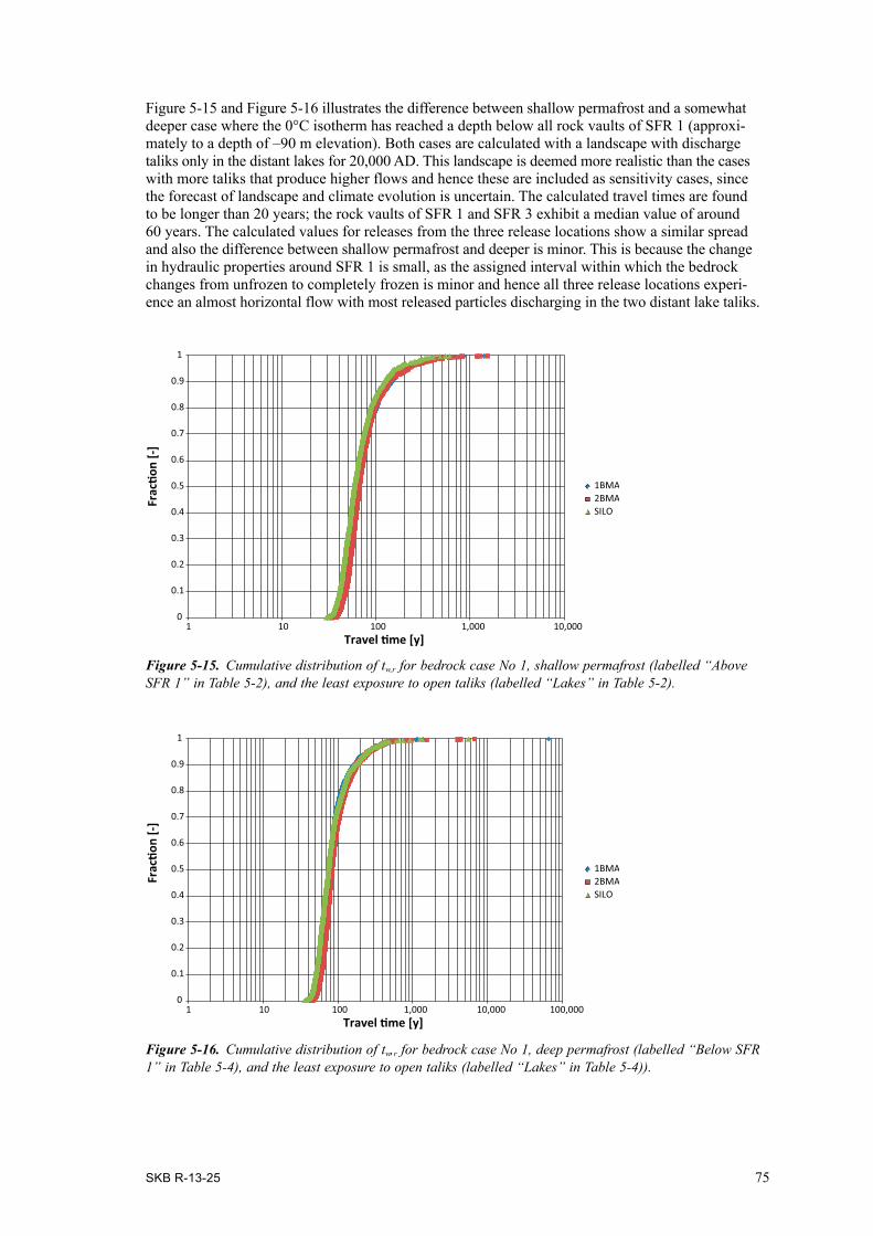
SKB R-13-25 75

Figure 5-15 and Figure 5-16 illustrates the difference between shallow permafrost and a somewhat deeper case where the 0°C isotherm has reached a depth below all rock vaults of SFR 1 (approxi-mately to a depth of –90 m elevation). Both cases are calculated with a landscape with discharge taliks only in the distant lakes for 20,000 AD. This landscape is deemed more realistic than the cases with more taliks that produce higher flows and hence these are included as sensitivity cases, since the forecast of landscape and climate evolution is uncertain. The calculated travel times are found to be longer than 20 years; the rock vaults of SFR 1 and SFR 3 exhibit a median value of around 60 years. The calculated values for releases from the three release locations show a similar spread and also the difference between shallow permafrost and deeper is minor. This is because the change in hydraulic properties around SFR 1 is small, as the assigned interval within which the bedrock changes from unfrozen to completely frozen is minor and hence all three release locations experi-ence an almost horizontal flow with most released particles discharging in the two distant lake taliks.

Figure 5-15. Cumulative distribution of tw,r for bedrock case No 1, shallow permafrost (labelled “Above SFR 1” in Table 5-2), and the least exposure to open taliks (labelled “Lakes” in Table 5-2).

Figure 5-16. Cumulative distribution of tw,r for bedrock case No 1, deep permafrost (labelled “Below SFR 1” in Table 5-4), and the least exposure to open taliks (labelled “Lakes” in Table 5-4)).

Frac

�on

[-]

0

0.1

0.2

0.3

0.4

0.5

0.6

0.7

0.8

0.9

1

1 10 100 1,000 10,000Travel �me [y]

1BMA2BMASILO

Frac

�on

[-]

0

0.1

0.2

0.3

0.4

0.5

0.6

0.7

0.8

0.9

1

1 10 100 1,000 10,000 100,000Travel �me [y]

1BMA2BMASILO

76 SKB R-13-25

5.5.6 Path lengthFigure 5-17 to Figure 5-19 below show cumulative distribution (probability) plots of the discharge path lengths for all the released particles divided into release from different rock vaults. Figure 5-17 illustrates the results for a release in a landscape affected by shallow permafrost; with a 0°C isotherm at approximately –60 m elevation . Additionally, the landscape is assumed to have a large number of taliks. Taliks are assumed in all peat-filled depressions and small ponds within the model domain along with the streams and lakes at 20,000 AD. The calculated path lengths are found to be larger than 400 m; the rock vaults of SFR 1 exhibit a median value of around 600 m, whereas the rock vaults of SFR 3 exhibit a median value of around 2,000 m.

The particles travelling from SFR 1 and the Silo exhibit a slight shift in the distribution plot at about 90% and 70% respectively. This shift is also apparent for the Silo in the less exposed landscape cases illustrated in Figure 5-18 and Figure 5-19 . The shift is primary related to some particles taking a somewhat deeper route towards the discharge locations. In the assessed models, this effect is exag-gerated due to the omission of brackish waters at depth.

Figure 5-18 and Figure 5-19 illustrate the difference between shallow permafrost and a somewhat deeper case where the 0°C isotherm has reached a depth below all rock vaults of SFR 1 (approxi-mately to a depth of –90 m elevation). Both cases are calculated with a landscape with discharge taliks only in the distant lakes that are for 20,000 AD. This landscape is deemed more realistic than the more talik-exposed cases that produce higher flows and hence these are included as sensitiv-ity cases, since the forecast of landscape and climate evolution are uncertain. The calculated path lengths are found to be larger than 200 m; the rock vaults of SFR 1 and SFR 3 exhibit a median value of around 10,000 m. The calculated values for releases from the three release locations show similar spread and also the difference between shallow permafrost and deeper is minor, except for a slightly lower number of particles from SFR 1 escaping through the permafrost in the deeper per-mafrost case. The minor difference is because the change in hydraulic properties around SFR 1 is small, because the assigned interval within which the bedrock changes from unfrozen to completely frozen is minor and hence all three release locations experience an almost horizontal flow with most released particles discharging in the two distant lake taliks.

Figure 5-17. Cumulative distribution of Lr for bedrock case No 1, shallow permafrost (labelled “Above SFR 1” in Table 5-2), and a high exposure to open taliks (labelled “All” in Table 5-2).

0

0.1

0.2

0.3

0.4

0.5

0.6

0.7

0.8

0.9

1

10 100 1,000 10,000 100,000

Frac

�on

[-]

Flow path length [m]

1BMA2BMASILO

SKB R-13-25 77

Figure 5-18. Cumulative distribution of Lr for bedrock case No 1, shallow permafrost (labelled “Above SFR 1” in Table 5-2), and the least exposure to open taliks (labelled “Lakes” in Table 5-2).

Figure 5-19. Cumulative distribution of Lr for bedrock case No 1, deep permafrost (labelled “Below SFR 1” in Table 5-2), and the least exposure to open taliks (labelled “Lakes” in Table 5-2).

0

0.1

0.2

0.3

0.4

0.5

0.6

0.7

0.8

0.9

1

10 100 1,000 10,000 100,000

Frac

�on

[-]

Flow path length [m]

1BMA2BMASILO

0

0.1

0.2

0.3

0.4

0.5

0.6

0.7

0.8

0.9

1

10 100 1,000 10,000 100,000

Frac

�on

[-]

Flow path length [m]

1BMA2BMASILO

SKB R-13-25 79

6 Integration of climate conditions and disciplines

The modelling studies deal with different climate conditions. In order to assess the full time evolu-tion in the dose calculations, the results from the different climate conditions have to be combined. It is therefore important to check the consistency between models used for temperate and periglacial conditions.

Below, a brief listing is also made of the other disciplines within SR-PSU where properties and results from the bedrock hydrogeological modelling are used.

6.1 Consistency between models used for flow modeling during temperate and periglacial climate conditions

In both TD11 (Öhman et al. 2014) and TD13 (Vidstrand et al. 2014), tunnel cross flows are calcu-lated for temperate climate conditions for the Base Case with a shoreline far away from the SFR repository. Hence, comparisons of these cases can be made and light can be shed on the consistency in results.

Figure 6-1 illustrates the rather limited differences between two types of top boundary condi-tions. In the permafrost simulations the top boundary condition was set as a specified pressure, with atmospheric pressure at the ground surface. The idea behind this assumption is that during the cold and dry conditions of permafrost, enough water is still available to maintain a ground water table or, more correctly stated, saturated conditions at the ground surface at all times. However, under temperate conditions the permeability of the ground may not be the limiting factor deter-mining the recharge. Hence, in this type of environment, the specified pressure top boundary con-dition set at the ground surface may induce local flow cells that would not occur in practice. The so-called “BaseCase Hybrid” results illustrated in Figure 6-1 are taken from the temperate simula-tions reported in Chapter 4 whereas the so-called “BaseCase Pressure” results are the results from the permafrost modelling without a frozen ground condition. The “BaseCase Pressure” boundary conditions yield somewhat larger cross flows, but the differences illustrated in Figure 6-1 are small and are not of any practical significance.

Figure 6-1. Comparison of resulting cross flows for two types of top boundary conditions.

80 SKB R-13-25

The simplification of the top boundary condition in groundwater flow simulations of the periglacial climate condition is primarily done for numerical reasons. But the assumption of a groundwater table at the ground surface has been identified and validated by other investigations. Bosson et al. (2012) investigated periglacial influences on the hydrology and concluded that even the cold and dry climate occurring during permafrost conditions could create a hydrological system with higher groundwater levels than during temperate conditions. Person et al. (2007) concluded that the unfrozen water content under permafrost conditions is sufficient to maintain the groundwater table at or close to the surface.

6.2 Use of hydrogeological properties and results in other disciplines within SR-PSU

Below is a summary of the hydrogeological properties and results from the bedrock hydrogeological simulations that are used by other disciplines within SR- PSU.

6.2.1 Near fieldThe upscaled hydraulic conductivity field of the bedrock from DarcyTools is exported for use in the near-field flow modelling to study the flow inside the rock vaults in more detail (Abarca et al. 2013). To set up the near-field flow model in COMSOL, boundary conditions, in terms of driving pressure fields and fluxes, are exported from DarcyTools.

6.2.2 Biosphere analysesThe locations of particles exiting the hydrogeological model of the bedrock at the bedrock/regolith interface are used as input in the biosphere analysis when identifying important biosphere objects in space and time (see the Biosphere synthesis report). Biosphere object 157_2 has been identified as a discharge area of great interest. A backward-particle tracking analysis was therefore carried out to determine the recharge locations of discharging groundwater, and the amount of groundwater dis-charging in object 157_2 that passed through the SFR facility, see Section 4.5.4.

6.2.3 Surface hydrologySurface hydrology and near-surface hydrogeology are modelled with the modelling tool MIKE SHE (Werner et al. 2013). The upscaled hydraulic properties of the bedrock (hydraulic conductivity, specific storage and porosity) are exported from DarcyTools to MIKE SHE for the hydrogeologi-cal Case 1 (see Table 4-4). Furthermore, exit locations from the DarcyTools model at the bedrock/ regolith interface as well as release points from the repository have been exported to MIKE SHE for the study of flow paths and travel times in the surface system.

To check the consistency between DarcyTools and MIKE SHE, the groundwater flow from the bed-rock to the biosphere objects during temperate conditions was calculated in DarcyTools and com-pared with corresponding results from MIKE SHE (Biosphere synthesis report). Furthermore, exit locations were also compared in Werner et al. (2013) and demonstrated a good consistency between the two models.

6.2.4 Far field Radionuclide transportThe radionuclide transport calculations are described in detail in the Radionuclide transport report. In the near-field calculations, the input comes from the detailed near-field modelling performed in COMSOL (see Section 6.2.1). In the far-field calculations, the inputs delivered from DarcyTools are the advective travel time and flow-related transport resistance in the bedrock.

6.2.5 Geochemical analysesRreactive transport modelling were carried out using the information about the recharge/discharge locations and the advective travel times in the bedrock (Román Ross et al. 2014). This informa-tion was coupled to the relevant geochemical processes in simulations performed following the FASTREACT methodology (Trinchero et al. 2014).

SKB R-13-25 81

7 Summary and conclusions

The present report summarises the methodology, setup, and results of the groundwater flow model-ling tasks performed within the SR-PSU project. Two different climate domains have been studied with regard to bedrock hydrogeology in the Forsmark-SFR area; temperate and peri glacial. Below, assumptions and conclusions with relevance for further use in the safety assessment SR-PSU are collated. Conclusions at the technical level associated with the numerical modelling of the two climate conditions are presented the individual modelling documents (Öhman et al. 2014, Vid-strand et al. 2014). The inter-disciplinary modelling using data acquired from site investigations and the integrated understanding of the Forsmark-SFR site is described in the SDM-PSU report (SKB 2013).

The following assumptions have been made in SR-PSU with respect to bedrock groundwater flow modelling:

• It is not necessary to consider variable-density flow (see Section 3.2.1 for motives);

• Fractured crystalline rock can be modelled as an anisotropic and heterogeneous continuum using the volumetric up-scaling algorithm imbedded in the DarcyTools modelling tool (Svensson 2010, Svensson and Ferry 2010, Svensson et al. 2010).

• The combination of heterogeneity and conceptual uncertainty in the bedrock parameterisation can be addressed and analysed in terms of a sensitivity analysis. It is assumed that the model perfor-mance can be evaluated for a selection of 17 different bedrock cases (cf. Table 4-5) and for six stages of shoreline displacement.

• The hydraulic properties of each regolith layer have been regarded as constant over geological time whereas the geometric properties were changed as specified in the landscape evolution mod-elling and the near-surface flow modelling (see Section 4.3.1 for details).

• Although the boundary conditions handled in the periglacial groundwater flow modelling are uncertain they are considered to encompass the range of possible conditions (Vidstrand et al. 2010).

The key performance measures (output) from the groundwater flow modelling are:

• Disposal room cross flows;

• Exit locations at the bedrock/regolith interface;

• Flow-related transport resistances in the bedrock along pathways determined by particle tracking;

• Advective travel times in the bedrock along flow paths determined by particle tracking.

A performance measure of supporting character is:

• Path lengths in the bedrock along pathways determined by particle tracking.

The results for each bedrock case and time slice have been exported to different users with SR-PSU.

The main conclusions from the study of the period with temperate climate conditions are the following.

• The discharge from the repository evolves over time. Before 3500 AD, exit locations are essentially adjacent to the Baltic Sea shoreline. The flow regime changes from upward-directed, during early time slices, to increasingly horizontal, at later time slices. The pattern of exit locations from SFR 1 appears stationary between time slices at 5000 AD and 9000 AD and, in essence, all particles dis-charge to biosphere object 157_2. During the early stages, SFR 3 has exit locations both north and south of the SFR pier. As the horizontal component in the flow regime successively grows, the exit locations are driven north, most particles discharge into biosphere object 157_2, although owing to its deeper location, a smaller number of particles discharge to biosphere objects related to biosphere object 116.

82 SKB R-13-25

• The tunnel cross flow increases during the early stages of shoreline displacement, to reach approximate stationary conditions at 5000 AD. From 3000 AD, 1BLA and 1BMA stand out with higher cross flows; this is probably related to their intersection with deformation zone ZFMNNW1209 (formerly referred to as Zone 6). Among the SFR 3 rock vaults, 2BMA stand out with higher cross flows. However, 4BLA and 5BLA also crosses the deformation zone ZFMWNW0835, and could, depending on HCD realisation, also have high cross flows.

• Flow paths tend to become longer with the retreating shoreline. This generally implies longer travel times and larger flow-related transport resistance values with time.

The main conclusions from the study of the period with periglacial climate conditions are as follows.

• During periglacial climate conditions the most relevant scenarios for the Forsmark-SFR site area reduces the total flow through the rock vaults and lengthen the path lengths, travel times and flow-related transport resistance values significantly increased compared with the values in temperate conditions. However, the climate conditions are uncertain and results are strongly dependent on the extent and number of taliks in the flow domain. In consequence, some of the rock vaults may experience small increases in total flows in periglacial relative to temperate conditions.

• The uncertainty in total flows associated with studied alternative periglacial climate conditions is not larger than the uncertainty arising from the different bedrock cases.

• The exit locations and flow-related transport properties are less affected by the uncertainty in bedrock properties. Instead, for all scenarios, the exit locations are controlled by the predefined open talik locations, where discharges are possible.

SKB R-13-25 83

References

SKB’s (Svensk Kärnbränslehantering AB) publications can be found at www.skb.se/publications. References to SKB’s unpublished documents are listed separately at the end of the reference list. Unpublished documents will be submitted upon request to document@skb.se.

References with abbreviated namesBiosphere synthesis report, 2014. Biosphere synthesis report for the safety assessment SRPSU. SKB TR-14-06, Svensk Kärnbränslehantering AB.

Climate report, 2014. Climate and climate related issues for the safety assessment SR-PSU. SKB TR-13-05, Svensk Kärnbränslehantering AB.

Data report, 2014. Data report for the for the safety assessment SR-PSU. SKB TR-14-10, Svensk Kärnbränslehantering AB.

Geosphere process report, 2014. Geosphere process report for the safety assessment SR-PSU. SKB TR-14-05, Svensk Kärnbränslehantering AB.

Initial state report, 2014. Initial state report for the safety assessment SR-PSU. SKB TR-14-02, Svensk Kärnbränslehantering AB.

Input data report, 2014. Input data report for the safety assessment SR-PSU. SKB TR-14-12, Svensk Kärnbränslehantering AB.

Model summary report, 2014. Model summary report for the safety assessment SR-PSU. SKB TR-14-11, Svensk Kärnbränslehantering AB.

Radionuclide transport report, 2014. Radionuclide transport and dose calculations for the safety assessment SR-PSU. SKB TR-14-09, Svensk Kärnbränslehantering AB.

SR-PSU Main report, 2014. Safety analysis for SFR. Long-term safety. Main report for the safety assessment SR-PSU. SKB TR-14-01, Svensk Kärnbränslehantering AB.

Other public referencesAbarca E, Idiart A, de Vries L M, Silva O, Molinero J, von Schenk H, 2013. Flow modelling on the repository scale for the safety assessment SR-PSU. SKB TR-13-08, Svensk Kärnbränsle-hantering AB.

Axelsson C-L, Ekstav A, Lindblad Påsse A, 2002. SFR – Utvärdering av hydrogeologi. SKB R-02-14, Svensk Kärnbränslehantering AB. (In Swedish.)

Bense V F, Person M A, 2008. Transient hydrodynamics within intercratonic sedimentary basins during glacial cycles. Journal of Geophysical Research 113, F04005. doi:10.1029/2007JF000969

Bosson E, Sassner M, Sabel U, Gustafsson L-G, 2010. Modelling of present and future hydro-logy and solute transport at Forsmark. SR-Site Biosphere. SKB R-10-02, Svensk Kärnbränsle-hantering AB.

Bosson E, Sabel U, Gustafsson L-G, Sassner M, Destouni G, 2012. Influences of shifts in cli-mate, landscape, and permafrost on terrestrial hydrology. Journal of Geophysical Research 117. doi: 10.1029/2011JD016429

Boulton G S, Slot T, Blessing P, Glasbergen T L, van Gijssel K, 1993. Deep circulation of groundwater in overpressured subglacial aquifers and its geological consequences. Quaternary Science Reviews 12, 739–745.

Brandefelt J, Näslund J-O, Zhang Q, Hartikainen J, 2013. The potential for cold climate conditions and permafrost in Forsmark in the next 60,000 years. SKB TR-13-04, Svensk Kärnbränslehantering AB.

84 SKB R-13-25

Brydsten L, Strömgren M, Löfgren A, Sohlenius G, Hartz F, 2013. Landscape development in the Forsmark area from the past into the future (8500 BC – 40000 AD). SKB R-13-27, Svensk Kärnbränslehantering AB.

Burt T P, Williams P J, 1976. Hydraulic conductivity in frozen soils. Earth Surface Processes 1, 349–360.

Carlsson L, Winberg A, Arnefors J, 1986. Hydraulic modeling of the final repository for reactor waste (SFR). Compilation and conceptualization of available geological and hydrogeological data. SKB SFR 86-03, Svensk Kärnbränslehantering AB.

Carlsson L, Winberg A, Grundfelt B, 1987. Hydraulic modelling of the final repository for reac-tor waste (SFR). Evaluation of the groundwater flow situation at SFR. SKB SFR 86-07, Svensk Kärnbränslehantering AB.

COMSOL, 2012. COMSOL Multiphysics, version 4.3a. Burlington, MA: COMSOL Inc.

Curtis P, Markström I, Petersson J, Triumf C-A, Isaksson H, Mattsson H, 2011. Site investiga-tion SFR. Bedrock geology. SKB R-10-49, Svensk Kärnbränslehantering AB.

de Marsily G, 1986. Quantitative hydrogeology: groundwater hydrology for engineers. Orlando, FL: Academic Press.

Follin S, 2008. Bedrock hydrogeology Forsmark. Site descriptive modelling, SDM-Site Forsmark. SKB R-08-95, Svensk Kärnbränslehantering AB.

French H M, 1996. The periglacial environment. 2nd ed. Harlow: Longman.

Gascoyne M, 2000. A review of published literature on the effects of permafrost on the hydrogeo-chemistry of bedrock. Posiva 2000-09, Posiva Oy, Finland

Graham D N, Butts M B, 2005. Flexible, integrated watershed modelling with MIKE SHE. In Singh V P, Frevert D K (eds). Watershed models. Boca Raton: CRC Press, 245–272.

Haldorsen S, Heim M, 1999. An Arctic groundwater system and its dependence upon climate change: an example from Svalberg. Permafrost and Periglacial Processes 10, 137–149.

Haggerty R, Gorelick S M, 1995. Multiple-rate mass transfer for modelling diffusion and surface reactions in media with pore-scale heterogeneity. Water Resources Research 31, 2383–2400.

Hartikainen J, Kouhia R, Wallroth T, 2010. Permafrost simulations at Forsmark using a numerical 2D thermo-hydro-chemical model. SKB TR-09-17, Svensk Kärnbränslehantering AB.

Holmén J G, Stigsson M, 2001. Modelling of future hydrogeological conditions at SFR. SKB R-01-02, Svensk Kärnbränslehantering AB.

Joyce S, Simpson T, Hartley L, Applegate D, Hoek J, Jackson P, Swan D, Marsic N, Follin S, 2010. Groundwater flow modelling of periods with temperate climate conditions – Forsmark. SKBR-09-20, Svensk Kärnbränslehantering AB.

Kane D L, Stein J, 1983. Water movement into seasonally frozen soils. Water Resources Research 19, 1547–1557.

Kleinberg R L, Griffin D D, 2005. NMR measurements of permafrost: unfrozen water assay, pore-scale distribution of ice, and hydraulic permeability of sediments. Cold Regions Science and Technology 42, 63–77.

Lemieux J-M, Sudicky E A, Peltier W R, Tarasov L, 2008a. Simulating the impact of glaciations on continental groundwater flow systems: 1. Relevant processes and model formulation. Journal of Geophysical Research 113, F03017. doi:10.1029/2007JF000928

Lemieux J-M, Sudicky E A, Peltier W R, Tarasov L, 2008b. Simulating the impact of glaciations on continental groundwater flow systems: 2. Model application to the Wisconsinian glaciation over the Canadian landscape. Journal of Geophysical Research 113, F03018. doi:10.1029/2007JF000929

Lemieux J-M, Sudicky E A, Peltier W R, Tarasov L, 2008c. Dynamics of groundwater recharge and seepage over the Canadian landscape during the Wisconsinian glaciation. Journal of Geophysical Research 113, F01011. doi:10.1029/2007JF000838

SKB R-13-25 85

Lindborg T (ed), 2010. Landscape Forsmark – data, methodology and results for SR-Site. SKB TR-10-05, Svensk Kärnbränslehantering AB.

McEwen T, de Marsily G, 1991. The potential significance of permafrost to the behaviour of a deep radioactive waste repository. SKI Report 91:8, Statens kärnkraftinspekton (Swedish Nuclear Power Inspectorate).

Person M, McIntosh J, Bense V, Remenda V H, 2007. Pleistocene hydrology of North America: The role of ice sheets in reorganising groundwater flow systems. Reviews of Geophysics 45, 1–28.

Rhén I, Follin S, Hermanson J, 2003. Hydrogeological Site Descriptive Model – a strategy for its development during site investigations. SKB R-03-08, Svensk Kärnbränslehantering AB.

Román-Ross G, Trinchero P, Maia F, Molinero J, 2014. Hydrogeochemical modelling and proposed evolution of the groundwater types and processes in geosphere of SFR, SR-PSU. SKB R-13-30, Svensk Kärnbränslehantering AB.

Selroos J-O, Follin S. 2010. SR-Site groundwater flow modelling methodology, setup and results. SKB R-09-22, Svensk Kärnbränslehantering AB.

SKB, 2008a. Geovetenskapligt undersökningsprogram för utbyggnad av SFR. SKB R-08-67, Svensk Kärnbränslehantering AB. (In Swedish.)

SKB, 2008b. Site description of Forsmark at completion of the site investigation phase. SDM-Site Forsmark. SKB TR-08-05, Svensk Kärnbränslehantering AB.

SKB, 2013. Site description of the SFR area at Forsmark at completion of the site investigation phase, SDM-PSU Forsmark. SKB TR-11-04, Svensk Kärnbränslehantering AB.

Stephens M B, Fox A, La Pointe P, Simeonov A, Isaksson H, Hermanson J, Öhman J, 2007. Geology Forsmark. Site descriptive modelling Forsmark stage 2.2. SKB R-07-45, Svensk Kärnbränslehantering AB.

Stigsson M, Follin S, Andersson J, 1999. On the simulation of variable density flow at SFR, Sweden. SKB R-99-08, Svensk Kärnbränslehantering AB.

Sundberg J, Back P-E, Ländell M, Sundberg A, 2009. Modelling of temperature in deep bore-holes and evaluation of geothermal heat flow at Forsmark and Laxemar. SKB TR-09-14, Svensk Kärnbränslehantering AB.

Svensson U, 2010. DarcyTools version 3.4. Verification, validation and demonstration. SKB R-10-71, Svensk Kärnbränslehantering AB.

Svensson U, Ferry M, 2010. Darcy Tools version 3.4. User’s Guide. SKB R-10-72, Svensk Kärn-bränsle hantering AB.

Svensson U, Ferry M, Kuylenstierna H-O, 2010. DarcyTools version 3.4 – Concepts, methods and equations. SKB R-07-38, Svensk Kärnbränslehantering AB.

Trinchero P, Molinero J, Román-Ross G, 2014. FASTREACT – A streamline-based approach for the solution of multicomponent reactive transport problems. SKB R-10-45, Svensk Kärnbränslehantering AB.

Vidstrand P, 2003. Surface and subsurface conditions in permafrost areas – a literature review. SKB TR-03-06, Svensk Kärnbränslehantering AB.

Vidstrand P, Follin S, Zugec N, 2010. Groundwater flow modelling of periods with periglacial and glacial climate conditions – Forsmark. SKB R-09-21, Svensk Kärnbränslehantering AB.

Vidstrand P, Follin S, Selroos J-O, Näslund J-O, Rhén I, 2012. Modeling of groundwater flow at depth in crystalline rock beneath a moving ice-sheet margin, exemplified by the Fennoscandian Shield, Sweden. Hydrogeology Journal. doi: 10.1007/s10040-012-0921-8

Vidstrand P, Follin S, Öhman J, 2014. SR-PSU Hydrogeological modelling. TD13 – Periglacial climate conditions. SKB P-14-06, Svensk Kärnbränslehantering AB.

Walger E, Ludvigson J-E, Gentzschein B, 2010. SFR Site investigation. Evaluation of selected interference tests and pressure responses during drilling at SFR. SKB P-10-43, Svensk Kärnbränslehantering AB.

86 SKB R-13-25

Werner K, Sassner M, Johansson E, 2013. Hydrology and near-surface hydrogeology at Forsmark – synthesis for the SR-PSU project. SKB R-13-19, Svensk Kärnbränslehantering AB.

Williams P J, Smith M W, 1989. The frozen earth: fundamentals of geocryology. Cambridge: Cambridge University Press.

Öhman J, Follin S, 2010. Site investigation SFR. Hydrogeological modelling of SFR. Data review and parameterisation of model version 0.1. SKB P-09-49, Svensk Kärnbränslehantering AB.

Öhman J, Vidstrand P, 2014. SR-PSU Bedrock hydrogeology. TD12 – Water-supply wells in rock. SKB P-14-05, Svensk Kärnbränslehantering AB.

Öhman J, Bockgård N, Follin S, 2012. Site investigation SFR. Bedrock hydrogeology. SKB R-11-03, Svensk Kärnbränslehantering AB.

Öhman J, Follin S, Odén M, 2013. Site investigation SFR. Bedrock hydrogeology – Groundwater flow modelling. SKB R-11-10, Svensk Kärnbränslehantering AB.

Öhman J, Follin S, Odén M, 2014. SR-PSU Hydrogeological modelling. TD11 – Temperate climate conditions. SKB P-14-04, Svensk Kärnbränslehantering AB.

Unpublished documents

SKBdoc id, version Title Issuer, year

1395200 ver 1.0 TD05 – Effects in ECPM translation SKB, 20131395214 ver 2.0 TD08 – SFR 3 effect on the performance of the existing SFR 1 SKB, 20131395215 ver 1.0 TD10 – SFR 3 adaptation to hydrogeological conditions SKB, 20131395349 ver 1.0 TD06 – Density driven flow SKB, 2013

SKB R-13-25 87

Appendix A

DarcyToolsIn groundwater flow modeling during permafrost climate conditions it is necessary to account for freezing and thawing as the temperature changes. In effect, the mass conservation equation and the heat transport equation have to be modified in order incorporate phase changes. Also, material prop-erties such as permeability and thermal conductivity need to be modified to account for the freezing.

In reality, frozen ground is a four-phase system consisting of intact rock (with some kind of poros-ity), frozen fluid (ice), unfrozen fluid (water) and gases (air). Assuming that the pore space of the groundwater system is unchanged and filled with either ice or water, that is ignoring the possibility of a gaseous phase and simply adding the ice phase to a single fluid phase, a simplified ice content function ɛ [-] is employed:

φεφ

φεφ

)1( −=

=

f

i (Eq. A-1)

where φ i s the total kinematic porosity [–], φ i is the part of the kinematic porosity filled with ice, φ f

the part filled with water, and ɛ represents the ice content function. ɛ is generally assumed a continu-ous function of temperature and is given by:

( )( )

{ } 2

max

,min

exp1

−

=

−−=

wLL θθθβ

βεε

θ

θ

(Eq. A-2)

where ɛmax is the maximum value (generally assumed as 1), TL is the thawing temperature, and w is a thawing interval which has to be adopted to the simulated ground conditions (material) herein specified to 1 for a good approximation of bedrock. The thawing temperature is dependent on both the salinity and the pressure at the calculation point. In this study, however, these dependencies are ignored and the thawing temperature is fixed at zero degrees C.

In the present study, the permeability is assumed to be reduced by a power function of the unfrozen water content:

refkk α= (Eq. A-3)

with:

( )a)1(,max min εαα −= (Eq. A-4)

where the subscript ‘ref’ indicates the reference values associated with unfrozen conditions and αmin is a specified maximum reduction, herein assigned to five order of magnitude. It is noted that no information on α typical for fractured crystalline rocks has been found in the literature. Relations between temperature and hydraulic conductivity for different saturated frozen soils (typically silt and sand materials) are reported by Burt and Williams (1976). In this reference most of the tested materi-als seem to reach a plateau when approaching hydraulic conductivity values between 1·10–11 m/s and 1·10–13 m/s; i.e. the hydraulic conductivity does not seem to be further reduced with lower tempera-tures. Similar experimental data are also presented in Kleinberg and Griffin (2005).

The introduction of an ice phase dependent on the temperature links the conservation equations, which become non-linear. When the densities of the solid (ice) and fluid phase differ, there is a motion of the fluid due to changes in volumes. Incorporating these effects yields a mass conserva-tion equation as follows:

88 SKB R-13-25

Qwx

vy

uxtt fff

fif =∂∂+

∂∂+

∂∂+

∂−∂

+∂

∂)()()(

)(ρρρ

εφρρφρ (Eq. A-5)

where ρf is fluid density [ML–3], ρi is ice density [ML–3], t is time [T] (u, v, w) are the directional com-ponents of the volumetric (Darcy) flux q [LT–1] at the location (x, y, z) [L,L,L] in a Cartesian coordinate system, and Q is a source/sink term per unit volume of fluid mass [ML–3T–1]. The mass conservation equation is turned into a pressure equation by invoking the assumptions behind Darcy’s law:

( )gkzPkw

yPk

v

xPku

fzz

y

x

0ρρµµ

µ

µ

−−∂∂−=

∂∂−=

∂∂−=

(Eq. A-6)

where kx, ky and kz are the orthogonal components of the permeability tensor parallel to the Cartesian coordinate system [L2], μ is the fluid dynamic viscosity [ML–1T–1], g is the acceleration due to grav-ity [LT–2], ρ0 is a reference fluid density [ML–3], and P is the residual (dynamic) fluid pressure [ML–1T–2] at the location (x, y, z):

zgpP 0ρ+= (Eq. A-7)

where p is the gauge pressure [ML–1T–2] and ρ0 gz is the hydrostatic pressure, P0. The residual fluid pressure, P, is used for numerical reasons, i.e. in order to avoid storing large numbers in the compu-tations.

The hydraulic conductivity K [LT–1] is related to the permeability k through the relation:

kg

K f

µρ

= (Eq. A-8)

For variable-density flow at isothermal conditions, ρf and μ are given by the following state laws:

[ ]20201

2210 )()(1 θθβθθβααρρ −−−−++= CCf

(Eq. A-9)

[ ]γθθβθθβααµµ 20403

2430 )()(1 −+−+++= CC (Eq. A-10)

where α, β γ and μ0 are constants and C and θ represent the salinity (mass fraction) [–], herein the salinity is specified as zero, and the temperature [K] with θ0 set as zero degrees C.

Herein the parameters are given as:

ρ0 α1 α2 β1 β2

1,000 7.80·10–3 –1.18·10–4 5.73·10–5 3.70·10–6

μ0 α3 α4 β3 β4 γ

1.78·10–3 7.80·10–3 –1.18·10–4 –2.25·10–2 1.67·10–4 1.3

SKB R-13-25 89

and:

fTDSC ρ/= (Eq. A-11)

where TDS is the abbreviation of Total Dissolved Solids [ML–3]. The migration of salt is modeled in terms of advection and diffusion processes in the mobile pore system and as a diffusion process in an immobile (rock matrix) pore system, simulated by the multi-rate methodology (Haggerty and Gorelick 1995). The advection-diffusion equation for the mobile pore system is modeled according to the following equation:

Czff

yff

xff

QQCzCDwC

z

yCDvC

y

xCDuC

xtC

+=

∂∂−

∂∂+

∂∂−

∂∂+

∂∂−

∂∂+

∂∂

γρρ

γρρ

γρρρφ

(Eq. A-12)

with:

ερρρρ )( fif −+= (Eq. A-13)

where ɛ is given by (Eq. A-1). Dx, Dy and Dz are the orthogonal components of the diffusion tensor parallel to the Cartesian coordinate system [L2T–1], QC and QC are source/sink terms per unit volume of fluid mass [ML–3T–1], where QC represents the diffusive exchange of salt per unit volume of fluid mass between the mobile and immobile pore volumes [ML–3T–1] and where C is always the com-puted value, and γ is a dimensionless coefficient that describes the dependency of the kinematic porosity of the mobile pore system on the dynamic pressure:

γφφ 0= (Eq. A-14)

( )gPPS

f

s

ρφγ 0

0

1 −+= (Eq. A-15)

where Ss is the specific storage, including all compressibility effects of the conductive pore system [L–1], see e.g. de Marsily (1986).

The physical interpretation of the multi-rate diffusion model of Haggerty and Gorelick (1995) used is, in principle, to specify the penetration depth, Li [L], of each exchange rate coefficient, αi [T–1], as:

=

im

ei

DLαφ

2 (Eq. A-16)

where De [L2T–1] is an effective diffusion coefficient and øm is the matrix porosity [-].

The penetration depth of the remotest diffusive exchange rate is estimated by inserting the minimum exchange rate coefficient into Eq. 16. The value of the matrix porosity is estimated from the follow-ing relationship:

φβφ =m (Eq. A-17)

where β [-] is the ratio between the diffusive and advective pore spaces and φ is the grid cell kin-ematic porosity [-]. Inserting De = 4×10–15 – 4×10–14 m2/s, β = 10, αmin = 4×10–12 s–1 and φ = 1×10–4

(Joyce et al. 2010) render penetration depths of the remotest diffusive exchange rate that vary in the range of a few meters (2–6 m), that is, the penetration depth simulated here is limited.

It should be noted that in the present simulations herein reported the salinity is omitted.

90 SKB R-13-25

Assessing Eq. 4-1 the heat conservation equation may be written as:

Tpffff

zpff

ypff

xpff

iipf

Qczw

yv

xu

zwc

z

yvc

y

xuc

x

tL

tc

tc

tc

+

∂

∂+

∂∂

+∂

∂=

∂∂−

∂∂+

∂∂−

∂∂+

∂∂−

∂∂+

∂∂

∂∂−

∂∂+

∂−∂

+∂

∂

θρρρθλθρ

θλθρ

θλθρ

θφθερθφθφθ

ρφ)1(

(Eq. A-18)

with:

ερ )( pfpiii ccc −= (Eq. A-19)

where ε is given by (Eq. A-1), ρ is described by (Eq. A-13), q is the temperature [K], cpf is the spe-cific heat capacity of the fluid and cpi is the specific heat capacity of ice [L2T–2K–1] (or [J/(kg K)]), c is the specific heat capacity of the ground [L2T–2K–1] (or [J/(kg K)]), L is the specific latent heat [L2T–2(or J/kg)], and λx, λy and λz are the directional components of the equivalent (i.e. matrix with fluid) thermal conductivity tensor [MLT–3K–1] (or [W/(m K)]). QT represents a sink/source term [ML–

1T–3] ([or W/m3]). (Eq. A-19) is introduced since it corresponds to the numerical implementation in DarcyTools. One should note that Ci is not the thermal capacity of ice, but a numerical quantity.

The individual phases are assumed randomly distributed within a unit volume and, hence, the ther-mal conductivity is computed as a mean square root weighting of the three phases’ (matrix, fluid, ice) individual thermal conductivities. However, as the thermal conductivity of the matrix is not directly used, but instead the equivalent thermal conductivity of the unfrozen material, the thermal conductivity of frozen ground is computed as:

2))(( εφλλλλ firef −+= (Eq. A-20)

where λref is the equivalent thermal conductivity of the saturated matrix, λi is the ice thermal conduc-tivity and λf is the thermal conductivity of the fluid.