sql command

SQL

Structured Query

Language

compiled by : Mohammad Nasib Refa3e

Zarqa Private University

Software Engineering

20070375

Digitalstar89 @ hotmail.com

2009

This report was compiled by Mohammad Nasib Refa3e (2 )

content

Subject Page

Sql Select -------------------- 4

Sql Distinct -------------------- 4

Sql Where -------------------- 5

Sql And Or -------------------- 5

Sql In -------------------- 6

Sql Between -------------------- 7

Sql Like -------------------- 8

Sql Order By -------------------- 8

Sql Average -------------------- 10

Sql Count -------------------- 10

Sql Max -------------------- 11

Sql Min -------------------- 12

Sql Sum -------------------- 12

Sql Groub By -------------------- 13

Sql Having -------------------- 13

Sql Join -------------------- 14

Sql Outer Join -------------------- 15

Sql Concatenate -------------------- 16

Sql Substring -------------------- 17

Sql Trim -------------------- 18

Sql Length -------------------- 19

Sql Replace -------------------- 20

Sql Create Table -------------------- 21

Sql Not Null Constrant -------------------- 21

Sql Default Constrant -------------------- 22

Sql Unique Constrant -------------------- 22

Sql Check Constrant -------------------- 23

Sql Primary Key -------------------- 23

Sql Foreign Key -------------------- 24

Sql View -------------------- 25

Sql Create View -------------------- 26

Sql Alter Table -------------------- 27


Sql Drop Table -------------------- 29

Sql Truncate Table -------------------- 30

Sql Insert Unto -------------------- 30

Sql Update -------------------- 31

Sql Delete -------------------- 32

Sql Union -------------------- 33

Sql Union All -------------------- 34

Sql Intersect -------------------- 35

Sql Minus -------------------- 36

Sql Limit -------------------- 37

Sql Top -------------------- 38

Sql Subquery -------------------- 39

Sql Exists -------------------- 40

Sql Case -------------------- 42

Sql Null -------------------- 43

Sql Is Null -------------------- 43

Sql If Null -------------------- 44

Sql Nvl -------------------- 45

Sql Coalesce -------------------- 45

Sql Null If -------------------- 46

Sql Rank -------------------- 47

Sql Median -------------------- 48

Sql Runing Totals -------------------- 48

Sql Percent To Total -------------------- 49

Sql Cumulative Percent Total -------------------- 50

هبذا شاهد ودميلومعي امللوب اىل احلبيب متيللك ********

لدموع امعارفني تس يصارت ادلميل اذا ذكرت محمدا أ ما ********

رسول ملك امعاملنيهذا رسول هللا هرباس امهدىهذا ********

الاهدا

لك من يعشق هبينا محمد ) صىل هللا عليه وسمل (اىل

مثرة ل صبح روتينطاملا ة اميتامبذر اىل

لك من علمين وتعب من أ جًلاىل

وأ حهبم كليبمن هوامه اىل


SQL Command SQL SELECT :

SELECT "column_name" FROM "table_name" To illustrate the above example, assume that we have the following table:

Table Store_Information

store_name Sales Date

Los Angeles $1500 Jan-05-1999

San Diego $250 Jan-07-1999


Boston $700 Jan-08-1999

We shall use this table as an example throughout the tutorial (this table will appear in all sections). To select all the stores in this table, we key in,

SELECT store_name FROM Store_Information

Result:

store_name

Los Angeles

San Diego

Los Angeles

Boston

Multiple column names can be selected, as well as multiple table names.

SQL DISTINCT :

SELECT DISTINCT "column_name" FROM "table_name"

For example, to select all distinct stores in Table Store_Information,






Boston $700 Jan-08-1999

we key in,

http://www.1keydata.com/sql/sqlselect.html

http://www.1keydata.com/sql/sqldistinct.html


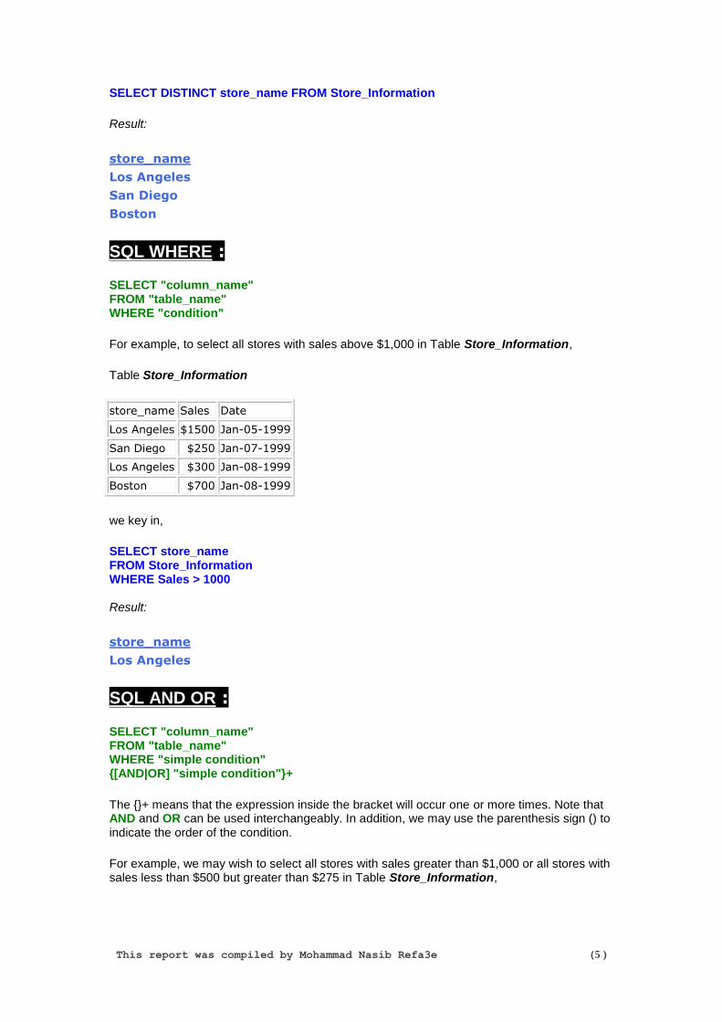
SELECT DISTINCT store_name FROM Store_Information

Result:

store_name

Los Angeles

San Diego

Boston

SQL WHERE :

SELECT "column_name" FROM "table_name" WHERE "condition"

For example, to select all stores with sales above $1,000 in Table Store_Information,






Boston $700 Jan-08-1999

we key in,

SELECT store_name FROM Store_Information WHERE Sales > 1000 Result:

store_name

Los Angeles

SQL AND OR :

SELECT "column_name" FROM "table_name" WHERE "simple condition" {[AND|OR] "simple condition"}+

The {}+ means that the expression inside the bracket will occur one or more times. Note that AND and OR can be used interchangeably. In addition, we may use the parenthesis sign () to indicate the order of the condition.

For example, we may wish to select all stores with sales greater than $1,000 or all stores with sales less than $500 but greater than $275 in Table Store_Information,

http://www.1keydata.com/sql/sqlwhere.html

http://www.1keydata.com/sql/sqlandor.html






San Francisco $300 Jan-08-1999

Boston $700 Jan-08-1999

we key in,

SELECT store_name FROM Store_Information WHERE Sales > 1000 OR (Sales < 500 AND Sales > 275) Result:

store_name

Los Angeles

San Francisco

SQL IN :

SELECT "column_name" FROM "table_name" WHERE "column_name" IN ('value1', 'value2', ...)

The number of values in the parenthesis can be one or more, with each values separated by comma. Values can be numerical or characters. If there is only one value inside the parenthesis, this commend is equivalent to

WHERE "column_name" = 'value1'

For example, we may wish to select all records for the Los Angeles and the San Diego stores in Table Store_Information,






Boston $700 Jan-08-1999

we key in,

http://www.1keydata.com/sql/sqlin.html


SELECT * FROM Store_Information WHERE store_name IN ('Los Angeles', 'San Diego')

Result:




SQL BETWEEN :

SELECT "column_name" FROM "table_name" WHERE "column_name" BETWEEN 'value1' AND 'value2'

This will select all rows whose column has a value between 'value1' and 'value2'.

For example, we may wish to select view all sales information between January 6, 1999, and January 10, 1999, in Table Store_Information,






Boston $700 Jan-08-1999

we key in,

SELECT * FROM Store_Information WHERE Date BETWEEN 'Jan-06-1999' AND 'Jan-10-1999'

Note that date may be stored in different formats in different databases. This tutorial simply choose one of the formats.

Result:




Boston $700 Jan-08-1999

http://www.1keydata.com/sql/sqlbetween.html


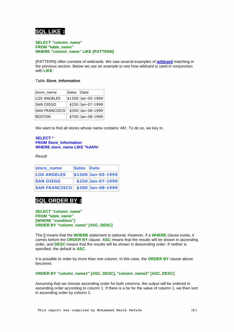
SQL LIKE :

SELECT "column_name" FROM "table_name" WHERE "column_name" LIKE {PATTERN}

{PATTERN} often consists of wildcards. We saw several examples of wildcard matching in the previous section. Below we use an example to see how wildcard is used in conjunction with LIKE:



LOS ANGELES $1500 Jan-05-1999

SAN DIEGO $250 Jan-07-1999

SAN FRANCISCO $300 Jan-08-1999

BOSTON $700 Jan-08-1999

We want to find all stores whose name contains 'AN'. To do so, we key in,

SELECT * FROM Store_Information WHERE store_name LIKE '%AN%' Result:


LOS ANGELES $1500 Jan-05-1999

SAN DIEGO $250 Jan-07-1999

SAN FRANCISCO $300 Jan-08-1999

SQL ORDER BY :

SELECT "column_name" FROM "table_name" [WHERE "condition"] ORDER BY "column_name" [ASC, DESC]

The [] means that the WHERE statement is optional. However, if a WHERE clause exists, it comes before the ORDER BY clause. ASC means that the results will be shown in ascending order, and DESC means that the results will be shown in descending order. If neither is specified, the default is ASC.

It is possible to order by more than one column. In this case, the ORDER BY clause above becomes

ORDER BY "column_name1" [ASC, DESC], "column_name2" [ASC, DESC]

Assuming that we choose ascending order for both columns, the output will be ordered in ascending order according to column 1. If there is a tie for the value of column 1, we then sort in ascending order by column 2.

http://www.1keydata.com/sql/sqllike.html

http://www.1keydata.com/sql/sql-wildcard.html

http://www.1keydata.com/sql/sqlorderby.html


For example, we may wish to list the contents of Table Store_Information by dollar amount, in descending order:






Boston $700 Jan-08-1999

we key in,

SELECT store_name, Sales, Date FROM Store_Information ORDER BY Sales DESC Result:



Boston $700 Jan-08-1999



In addition to column name, we may also use column position (based on the SQL query) to indicate which column we want to apply the ORDER BY clause. The first column is 1, second column is 2, and so on. In the above example, we will achieve the same results by the following command:

SELECT store_name, Sales, Date FROM Store_Information ORDER BY 2 DESC

SQL Aggregate Functions :

* AVG: Average of the column.

• COUNT: Number of records.

• MAX: Maximum of the column.

• MIN: Minimum of the column.

• SUM: Sum of the column.

http://www.1keydata.com/sql/sql-average.html

http://www.1keydata.com/sql/sqlcount.html

http://www.1keydata.com/sql/sql-max.html

http://www.1keydata.com/sql/sql-min.html

http://www.1keydata.com/sql/sql-sum.html


SQL Average :

The syntax for using functions is,

SELECT "function type" ("column_name") FROM "table_name"

SQL uses the AVG() function to calculate the average of a column. The syntax for using this function is,

SELECT AVG("column_name") FROM "table_name"

For example, if we want to get the average of all sales from the following table,






Boston $700 Jan-08-1999

we would type in

SELECT AVG(Sales) FROM Store_Information Result:

AVG(Sales)

$687.5

$687.5 represents the average of all Sales entries: ($1500 + $250 + $300 + $700) / 4.

SQL Count :

This allows us to COUNT up the number of row in a certain table. The syntax is,

SELECT COUNT("column_name") FROM "table_name"

For example, if we want to find the number of store entries in our table,






Boston $700 Jan-08-1999


we'd key in

SELECT COUNT(store_name) FROM Store_Information

Result:

Count(store_name)

4

COUNT and DISTINCT can be used together in a statement to fetch the number of distinct entries in a table. For example, if we want to find out the number of distinct stores, we'd type,

SELECT COUNT(DISTINCT store_name) FROM Store_Information

Result:

Count(DISTINCT store_name)

3

SQL MAX Function :

SQL uses the MAX function to find the maximum value in a column. The syntax for using the MAX function is,

SELECT MAX("column_name") FROM "table_name"

For example, if we want to get the highest sales from the following table,






Boston $700 Jan-08-1999

we would type in

SELECT MAX(Sales) FROM Store_Information Result:

MAX(Sales)

$1500

$1500 represents the maximum value of all Sales entries: $1500, $250, $300, and $700.


SQL MIN Function :

SQL uses the MIN function to find the maximum value in a column. The syntax for using the MIN function is,

SELECT MIN("column_name") FROM "table_name"

For example, if we want to get the lowest sales from the following table,






Boston $700 Jan-08-1999

we would type in

SELECT MIN(Sales) FROM Store_Information Result:

MIN(Sales)

$250

$250 represents the minimum value of all Sales entries: $1500, $250, $300, and $700.

SQL SUM Function ;

The SUM function is used to calculate the total for a column. The syntax is,

SELECT SUM("column_name") FROM "table_name"

For example, if we want to get the sum of all sales from the following table,






Boston $700 Jan-08-1999

we would type in


SELECT SUM(Sales) FROM Store_Information Result:

SUM(Sales)

$2750

$2750 represents the sum of all Sales entries: $1500 + $250 + $300 + $700.

SQL Group By :

SELECT "column_name1", SUM("column_name2") FROM "table_name" GROUP BY "column_name1"

Let's illustrate using the following table,






Boston $700 Jan-08-1999

We want to find total sales for each store. To do so, we would key in,

SELECT store_name, SUM(Sales) FROM Store_Information GROUP BY store_name

Result:

store_name SUM(Sales)

Los Angeles $1800

San Diego $250

Boston> $700

The GROUP BY keyword is used when we are selecting multiple columns from a table (or tables) and at least one arithmetic operator appears in the SELECT statement. When that happens, we need to GROUP BY all the other selected columns, i.e., all columns except the one(s) operated on by the arithmetic operator.

SQL HAVING :

Another thing people may want to do is to limit the output based on the corresponding sum (or any other aggregate functions). For example, we might want to see only the stores with sales over $1,500. Instead of using the WHERE clause in the SQL statement, though, we need to use the HAVING clause, which is reserved for aggregate functions. The HAVING clause is typically placed near the end of the SQL statement, and a SQL statement with the HAVING clause may or may not include the GROUP BY clause. The syntax for HAVING is,

http://www.1keydata.com/sql/sqlhaving.html


SELECT "column_name1", SUM("column_name2") FROM "table_name" GROUP BY "column_name1" HAVING (arithmetic function condition)

Note: the GROUP BY clause is optional.

In our example, table Store_Information,






Boston $700 Jan-08-1999

we would type,

SELECT store_name, SUM(sales) FROM Store_Information GROUP BY store_name HAVING SUM(sales) > 1500

Result:

store_name SUM(Sales)

Los Angeles $1800

SQL Join :






Boston $700 Jan-08-1999

Table Geography

region_name store_name

East Boston

East New York

West Los Angeles

West San Diego

and we want to find out sales by region. We see that table Geography includes information on regions and stores, and table Store_Information contains sales information for each store. To get the sales information by region, we have to combine the information from the


two tables. Examining the two tables, we find that they are linked via the common field, "store_name". We will first present the SQL statement and explain the use of each segment later:

SELECT A1.region_name REGION, SUM(A2.Sales) SALES FROM Geography A1, Store_Information A2 WHERE A1.store_name = A2.store_name GROUP BY A1.region_name

Result:

REGION SALES

East $700

West $2050

The first two lines tell SQL to select two fields, the first one is the field "region_name" from table Geography (aliased as REGION), and the second one is the sum of the field "Sales" from table Store_Information (aliased as SALES). Notice how the table aliases are used here: Geography is aliased as A1, and Store_Information is aliased as A2. Without the aliasing, the first line would become

SELECT Geography.region_name REGION, SUM(Store_Information.Sales) SALES

which is much more cumbersome. In essence, table aliases make the entire SQL statement easier to understand, especially when multiple tables are included.

Next, we turn our attention to line 3, the WHERE statement. This is where the condition of the join is specified. In this case, we want to make sure that the content in "store_name" in table Geography matches that in table Store_Information, and the way to do it is to set them equal. This WHERE statement is essential in making sure you get the correct output. Without the correct WHERE statement, a Cartesian Join will result. Cartesian joins will result in the query returning every possible combination of the two (or whatever the number of tables in the FROM statement) tables. In this case, a Cartesian join would result in a total of 4 x 4 = 16 rows being returned.

SQL Outer Join :

Previously, we had looked at left join, or inner join, where we select rows common to the participating tables to a join. What about the cases where we are interested in selecting elements in a table regardless of whether they are present in the second table? We will now need to use the SQL OUTER JOIN command. The syntax for performing an outer join in SQL is database-dependent. For example, in Oracle, we will place an "(+)" in the WHERE clause on the other side of the table for which we want to include all the rows.

Let's assume that we have the following two tables,






Boston $700 Jan-08-1999


Table Geography


East Boston

East New York

West Los Angeles

West San Diego

and we want to find out the sales amount for all of the stores. If we do a regular join, we will not be able to get what we want because we will have missed "New York," since it does not appear in the Store_Information table. Therefore, we need to perform an outer join on the two tables above:

SELECT A1.store_name, SUM(A2.Sales) SALES FROM Geography A1, Store_Information A2 WHERE A1.store_name = A2.store_name (+) GROUP BY A1.store_name

Note that in this case, we are using the Oracle syntax for outer join.

Result:

store_name SALES

Boston $700

New York

Los Angeles $1800

San Diego $250

Note: NULL is returned when there is no match on the second table. In this case, "New York" does not appear in the table Store_Information, thus its corresponding "SALES" column is NULL.

SQL Concatenate :

Sometimes it is necessary to combine together (concatenate) the results from several different fields. Each database provides a way to do this:

MySQL: CONCAT()

Oracle: CONCAT(), ||

SQL Server: +

The syntax for CONCAT() is as follows:

CONCAT(str1, str2, str3, ...): Concatenate str1, str2, str3, and any other strings together. Please note the Oracle CONCAT() function only allows two arguments -- only two strings can be put together at a time using this function. However, it is possible to concatenate more than two strings at a time in Oracle using '||'.

Let's look at some examples. Assume we have the following table:


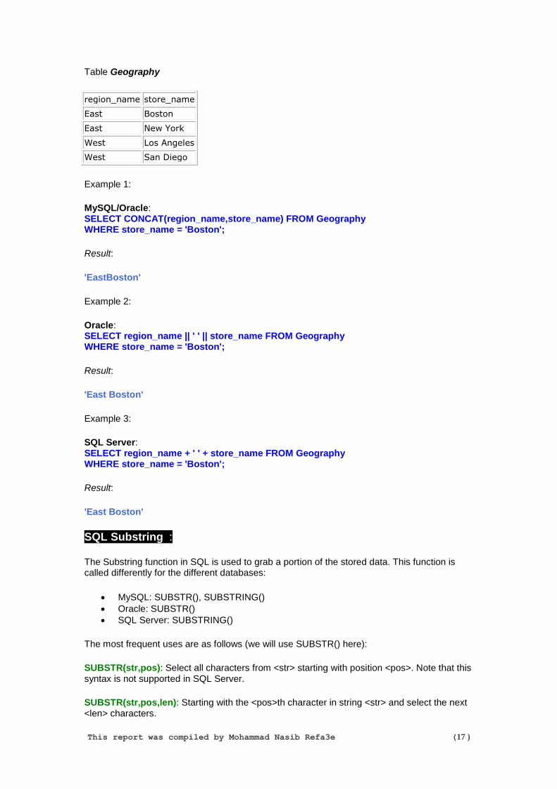
Table Geography


East Boston

East New York

West Los Angeles

West San Diego

Example 1:

MySQL/Oracle: SELECT CONCAT(region_name,store_name) FROM Geography WHERE store_name = 'Boston';

Result:

'EastBoston'

Example 2:

Oracle: SELECT region_name || ' ' || store_name FROM Geography WHERE store_name = 'Boston';

Result:

'East Boston'

Example 3:

SQL Server: SELECT region_name + ' ' + store_name FROM Geography WHERE store_name = 'Boston';

Result:

'East Boston'

SQL Substring :

The Substring function in SQL is used to grab a portion of the stored data. This function is called differently for the different databases:

MySQL: SUBSTR(), SUBSTRING()

Oracle: SUBSTR()

SQL Server: SUBSTRING()

The most frequent uses are as follows (we will use SUBSTR() here):

SUBSTR(str,pos): Select all characters from <str> starting with position <pos>. Note that this syntax is not supported in SQL Server.

SUBSTR(str,pos,len): Starting with the <pos>th character in string <str> and select the next <len> characters.


Assume we have the following table:

Table Geography


East Boston

East New York

West Los Angeles

West San Diego

Example 1:

SELECT SUBSTR(store_name, 3) FROM Geography WHERE store_name = 'Los Angeles';

Result:

's Angeles'

Example 2:

SELECT SUBSTR(store_name,2,4) FROM Geography WHERE store_name = 'San Diego';

Result:

'an D'

SQL Trim :

The TRIM function in SQL is used to remove specified prefix or suffix from a string. The most common pattern being removed is white spaces. This function is called differently in different databases:

MySQL: TRIM(), RTRIM(), LTRIM()

Oracle: RTRIM(), LTRIM()

SQL Server: RTRIM(), LTRIM()

The syntax for these trim functions are:

TRIM([[LOCATION] [remstr] FROM ] str): [LOCATION] can be either LEADING, TRAILING, or BOTH. This function gets rid of the [remstr] pattern from either the beginning of the string or the end of the string, or both. If no [remstr] is specified, white spaces are removed.

LTRIM(str): Removes all white spaces from the beginning of the string.

RTRIM(str): Removes all white spaces at the end of the string.


Example 1:

SELECT TRIM(' Sample ');

Result:

'Sample'

Example 2:

SELECT LTRIM(' Sample ');

Result:

'Sample '

Example 3:

SELECT RTRIM(' Sample ');

Result:

' Sample'

SQL Length ;

The Length function in SQL is used to get the length of a string. This function is called differently for the different databases:

MySQL: LENGTH()

Oracle: LENGTH()

SQL Server: LEN()

The syntax for the Length function is as follows:

Length(str): Find the length of the string str.

Let's take a look at some examples. Assume we have the following table:

Table Geography


East Boston

East New York

West Los Angeles

West San Diego


Example 1:

SELECT Length(store_name) FROM Geography WHERE store_name = 'Los Angeles';

Result: 11

Example 2: SELECT region_name, Length(region_name) FROM Geography;

Result:

region_name Length(region_name)

East 4

East 4

West 4

West 4

SQL Replace :

The Replace function in SQL is used to update the content of a string. The function call is REPLACE() for MySQL, Oracle, and SQL Server. The syntax of the Replace function is:

Replace(str1, str2, str3): In str1, find where str2 occurs, and replace it with str3.

Assume we have the following table:

Table Geography


East Boston

East New York

West Los Angeles

West San Diego

If we apply the following Replace function:

SELECT REPLACE(region_name, 'ast', 'astern') FROM Geography;

Result:

region_name

Eastern

Eastern

West

West


SQL Create Table Statement :

The SQL syntax for CREATE TABLE is

CREATE TABLE "table_name" ("column 1" "data_type_for_column_1", "column 2" "data_type_for_column_2", ... )

So, if we are to create the customer table specified as above, we would type in

CREATE TABLE customer (First_Name char(50), Last_Name char(50), Address char(50), City char(50), Country char(25), Birth_Date date)

SQL Constraint :

Common types of constraints include the following:

NOT NULL Constraint: Ensures that a column cannot have NULL value.

DEFAULT Constraint: Provides a default value for a column when none is specified.

UNIQUE Constraint: Ensures that all values in a column are different.

CHECK Constraint: Makes sure that all values in a column satisfy certain criteria.

Primary Key Constraint: Used to uniquely identify a row in the table.

Foreign Key Constraint: Used to ensure referential integrity of the data.

SQL NOT NULL Constraint :

By default, a column can hold NULL. If you not want to allow NULL value in a column, you will want to place a constraint on this column specifying that NULL is now not an allowable value.

For example, in the following statement,

CREATE TABLE Customer (SID integer NOT NULL, Last_Name varchar (30) NOT NULL, First_Name varchar(30));

Columns "SID" and "Last_Name" cannot include NULL, while "First_Name" can include NULL.

An attempt to execute the following SQL statement,

INSERT INTO Customer (Last_Name, First_Name) values ('Wong','Ken');

will result in an error because this will lead to column "SID" being NULL, which violates the NOT NULL constraint on that column.

http://www.1keydata.com/sql/sql-not-null.html

http://www.1keydata.com/sql/sql-default.html

http://www.1keydata.com/sql/sql-unique.html

http://www.1keydata.com/sql/sql-check.html

http://www.1keydata.com/sql/sql-primary-key.html

http://www.1keydata.com/sql/sql-foreign-key.html


SQL DEFAULT Constraint :

The DEFAULT constraint provides a default value to a column when the INSERT INTO statement does not provide a specific value. For example, if we create a table as below:

CREATE TABLE Student (Student_ID integer Unique, Last_Name varchar (30), First_Name varchar (30), Score DEFAULT 80);

and execute the following SQL statement,

INSERT INTO Student (Student_ID, Last_Name, First_Name) values ('10','Johnson','Rick');

The table will look like the following:

Student_ID Last_Name First_Name Score

10 Johnson Rick 80

Even though we didn't specify a value for the "Score" column in the INSERT INTO statement, it does get assigned the default value of 80 since we had already set 80 as the default value for this column.

SQL UNIQUE Constraint :

The UNIQUE constraint ensures that all values in a column are distinct.

For example, in the following CREATE TABLE statement,

CREATE TABLE Customer (SID integer Unique, Last_Name varchar (30), First_Name varchar(30));

column "SID" has a unique constraint, and hence cannot include duplicate values. Such constraint does not hold for columns "Last_Name" and "First_Name". So, if the table already contains the following rows:

SID Last_Name First_Name

1 Johnson Stella

2 James Gina

3 Aaron Ralph

Executing the following SQL statement,

INSERT INTO Customer values ('3','Lee','Grace');

will result in an error because '3' already exists in the SID column, thus trying to insert another row with that value violates the UNIQUE constraint.


Please note that a column that is specified as a primary key must also be unique. At the same time, a column that's unique may or may not be a primary key. In addition, multiple UNIQUE constraints can be defined on a table.

SQL CHECK Constraint :

The CHECK constraint ensures that all values in a column satisfy certain conditions. Once defined, the database will only insert a new row or update an existing row if the new value satisfies the CHECK constraint. The CHECK constraint is used to ensure data quality

For example, in the following CREATE TABLE statement,

CREATE TABLE Customer (SID integer CHECK (SID > 0), Last_Name varchar (30), First_Name varchar(30));

Column "SID" has a constraint -- its value must only include integers greater than 0. So, attempting to execute the following statement,

INSERT INTO Customer values ('-3','Gonzales','Lynn');

will result in an error because the values for SID must be greater than 0.

Please note that the CHECK constraint does not get enforced by MySQL at this time.

Primary Key :

A primary key is used to uniquely identify each row in a table. It can either be part of the actual record itself , or it can be an artificial field (one that has nothing to do with the actual record). A primary key can consist of one or more fields on a table. When multiple fields are used as a primary key, they are called a composite key.

Primary keys can be specified either when the table is created (using CREATE TABLE) or by changing the existing table structure (using ALTER TABLE).

Below are examples for specifying a primary key when creating a table:

MySQL: CREATE TABLE Customer (SID integer, Last_Name varchar(30), First_Name varchar(30), PRIMARY KEY (SID));

Oracle: CREATE TABLE Customer (SID integer PRIMARY KEY, Last_Name varchar(30), First_Name varchar(30));

SQL Server: CREATE TABLE Customer (SID integer PRIMARY KEY, Last_Name varchar(30), First_Name varchar(30));

http://www.1keydata.com/sql/sqlcreate.html

http://www.1keydata.com/sql/sql-alter-table.html


Below are examples for specifying a primary key by altering a table:

MySQL: ALTER TABLE Customer ADD PRIMARY KEY (SID);

Oracle: ALTER TABLE Customer ADD PRIMARY KEY (SID);

SQL Server: ALTER TABLE Customer ADD PRIMARY KEY (SID);

Note: Before using the ALTER TABLE command to add a primary key, you'll need to make sure that the field is defined as 'NOT NULL' -- in other words, NULL cannot be an accepted value for that field.

Foreign Key :

structure of these two tables will be as follows:

Table CUSTOMER

column name characteristic

SID Primary Key

Last_Name

First_Name

Table ORDERS

column name characteristic

Order_ID Primary Key

Order_Date

Customer_SID Foreign Key

Amount

In the above example, the Customer_SID column in the ORDERS table is a foreign key pointing to the SID column in the CUSTOMER table.

Below we show examples of how to specify the foreign key when creating the ORDERS table:

MySQL: CREATE TABLE ORDERS (Order_ID integer, Order_Date date, Customer_SID integer, Amount double, Primary Key (Order_ID), Foreign Key (Customer_SID) references CUSTOMER(SID));


Oracle: CREATE TABLE ORDERS (Order_ID integer primary key, Order_Date date, Customer_SID integer references CUSTOMER(SID), Amount double);

SQL Server: CREATE TABLE ORDERS (Order_ID integer primary key, Order_Date datetime, Customer_SID integer references CUSTOMER(SID), Amount double);

Below are examples for specifying a foreign key by altering a table. This assumes that the ORDERS table has been created, and the foreign key has not yet been put in:

MySQL: ALTER TABLE ORDERS ADD FOREIGN KEY (customer_sid) REFERENCES CUSTOMER(SID);

Oracle: ALTER TABLE ORDERS ADD (CONSTRAINT fk_orders1) FOREIGN KEY (customer_sid) REFERENCES CUSTOMER(SID);

SQL Server: ALTER TABLE ORDERS ADD FOREIGN KEY (customer_sid) REFERENCES CUSTOMER(SID);

SQL View :

A view is a virtual table. A view consists of rows and columns just like a table. The difference between a view and a table is that views are definitions built on top of other tables (or views), and do not hold data themselves. If data is changing in the underlying table, the same change is reflected in the view. A view can be built on top of a single table or multiple tables. It can also be built on top of another view. In the SQL Create View page, we will see how a view can be built.

Views offer the following advantages:

1. Ease of use: A view hides the complexity of the database tables from end users. Essentially we can think of views as a layer of abstraction on top of the database tables.

2. Space savings: Views takes very little space to store, since they do not store actual data.

3. Additional data security: Views can include only certain columns in the table so that only the non-sensitive columns are included and exposed to the end user. In addition, some databases allow views to have different security settings, thus hiding sensitive data from prying eyes.

http://www.1keydata.com/sql/sql-create-view.html


SQL Create View Statement :

Views can be considered as virtual tables. Generally speaking, a table has a set of definition, and it physically stores the data. A view also has a set of definitions, which is build on top of table(s) or other view(s), and it does not physically store the data.

The syntax for creating a view is as follows:

CREATE VIEW "VIEW_NAME" AS "SQL Statement"

"SQL Statement" can be any of the SQL statements we have discussed in this tutorial.

Let's use a simple example to illustrate. Say we have the following table:

TABLE Customer (First_Name char(50), Last_Name char(50), Address char(50), City char(50), Country char(25), Birth_Date date)

and we want to create a view called V_Customer that contains only the First_Name, Last_Name, and Country columns from this table, we would type in,

CREATE VIEW V_Customer AS SELECT First_Name, Last_Name, Country FROM Customer

Now we have a view called V_Customer with the following structure:

View V_Customer (First_Name char(50), Last_Name char(50), Country char(25))

We can also use a view to apply joins to two tables. In this case, users only see one view rather than two tables, and the SQL statement users need to issue becomes much simpler. Let's say we have the following two tables:






Boston $700 Jan-08-1999


Table Geography


East Boston

East New York

West Los Angeles

West San Diego

and we want to build a view that has sales by region information. We would issue the following SQL statement:

CREATE VIEW V_REGION_SALES AS SELECT A1.region_name REGION, SUM(A2.Sales) SALES FROM Geography A1, Store_Information A2 WHERE A1.store_name = A2.store_name GROUP BY A1.region_name

This gives us a view, V_REGION_SALES, that has been defined to store sales by region records. If we want to find out the content of this view, we type in,

SELECT * FROM V_REGION_SALES

Result:

REGION SALES

East $700

West $2050

SQL Alter Table Statement :

Once a table is created in the database, there are many occasions where one may wish to change the structure of the table. Typical cases include the following:

- Add a column - Drop a column - Change a column name - Change the data type for a column

Please note that the above is not an exhaustive list. There are other instances where ALTER TABLE is used to change the table structure, such as changing the primary key specification or adding a unique constraint to a column. The SQL syntax for ALTER TABLE is

ALTER TABLE "table_name" [alter specification]

[alter specification] is dependent on the type of alteration we wish to perform. For the uses cited above, the [alter specification] statements are:

Add a column: ADD "column 1" "data type for column 1"

Drop a column: DROP "column 1"

Change a column name: CHANGE "old column name" "new column name" "data type for new column name"

Change the data type for a column: MODIFY "column 1" "new data type"


Let's run through examples for each one of the above, using the "customer" table created in the CREATE TABLE section:

Table customer

Column Name Data Type

First_Name char(50)

Last_Name char(50)

Address char(50)

City char(50)

Country char(25)

Birth_Date date

First, we want to add a column called "Gender" to this table. To do this, we key in:

ALTER table customer add Gender char(1)

Resulting table structure:

Table customer


First_Name char(50)

Last_Name char(50)

Address char(50)

City char(50)

Country char(25)

Birth_Date date

Gender char(1)

Next, we want to rename "Address" to "Addr". To do this, we key in,

ALTER table customer change Address Addr char(50)


Table customer


First_Name char(50)

Last_Name char(50)

Addr char(50)

City char(50)

Country char(25)

Birth_Date date

Gender char(1)



Then, we want to change the data type for "Addr" to char(30). To do this, we key in,

ALTER table customer modify Addr char(30)


Table customer


First_Name char(50)

Last_Name char(50)

Addr char(30)

City char(50)

Country char(25)

Birth_Date date

Gender char(1)

Finally, we want to drop the column "Gender". To do this, we key in,

ALTER table customer drop Gender


Table customer


First_Name char(50)

Last_Name char(50)

Addr char(30)

City char(50)

Country char(25)

Birth_Date date

SQL Drop Table Statement :

Sometimes we may decide that we need to get rid of a table in the database for some reason. In fact, it would be problematic if we cannot do so because this could create a maintenance nightmare for the DBA's. Fortunately, SQL allows us to do it, as we can use the DROP TABLE command. The syntax for DROP TABLE is

DROP TABLE "table_name"

So, if we wanted to drop the table called customer that we created in the CREATE TABLE section, we simply type

DROP TABLE customer.



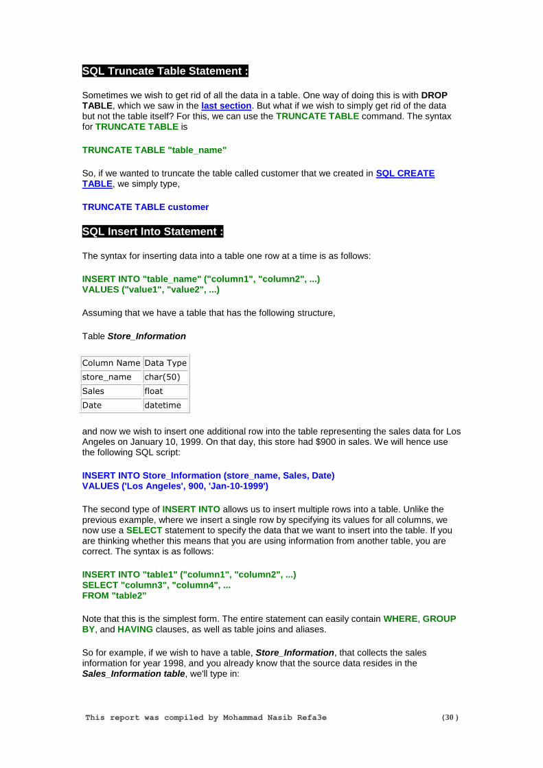
SQL Truncate Table Statement :

Sometimes we wish to get rid of all the data in a table. One way of doing this is with DROP TABLE, which we saw in the last section. But what if we wish to simply get rid of the data but not the table itself? For this, we can use the TRUNCATE TABLE command. The syntax for TRUNCATE TABLE is

TRUNCATE TABLE "table_name"

So, if we wanted to truncate the table called customer that we created in SQL CREATE TABLE, we simply type,

TRUNCATE TABLE customer

SQL Insert Into Statement :

The syntax for inserting data into a table one row at a time is as follows:

INSERT INTO "table_name" ("column1", "column2", ...) VALUES ("value1", "value2", ...)

Assuming that we have a table that has the following structure,



store_name char(50)

Sales float

Date datetime

and now we wish to insert one additional row into the table representing the sales data for Los Angeles on January 10, 1999. On that day, this store had $900 in sales. We will hence use the following SQL script:

INSERT INTO Store_Information (store_name, Sales, Date) VALUES ('Los Angeles', 900, 'Jan-10-1999')

The second type of INSERT INTO allows us to insert multiple rows into a table. Unlike the previous example, where we insert a single row by specifying its values for all columns, we now use a SELECT statement to specify the data that we want to insert into the table. If you are thinking whether this means that you are using information from another table, you are correct. The syntax is as follows:

INSERT INTO "table1" ("column1", "column2", ...) SELECT "column3", "column4", ... FROM "table2"

Note that this is the simplest form. The entire statement can easily contain WHERE, GROUP BY, and HAVING clauses, as well as table joins and aliases.

So for example, if we wish to have a table, Store_Information, that collects the sales information for year 1998, and you already know that the source data resides in the Sales_Information table, we'll type in:

http://www.1keydata.com/sql/sqldrop.html




INSERT INTO Store_Information (store_name, Sales, Date) SELECT store_name, Sales, Date FROM Sales_Information WHERE Year(Date) = 1998

Here I have used the SQL Server syntax to extract the year information out of a date. Other relational databases will have different syntax. For example, in Oracle, you will use to_char(date,'yyyy')=1998.

SQL Update Statement :

The syntax for this is

UPDATE "table_name" SET "column_1" = [new value] WHERE {condition}

For example, say we currently have a table as below:






Boston $700 Jan-08-1999

and we notice that the sales for Los Angeles on 01/08/1999 is actually $500 instead of $300, and that particular entry needs to be updated. To do so, we use the following SQL:

UPDATE Store_Information SET Sales = 500 WHERE store_name = "Los Angeles" AND Date = "Jan-08-1999"

The resulting table would look like






Boston $700 Jan-08-1999

In this case, there is only one row that satisfies the condition in the WHERE clause. If there are multiple rows that satisfy the condition, all of them will be modified. If no WHERE clause is specified, all rows will be modified.


It is also possible to UPDATE multiple columns at the same time. The syntax in this case would look like the following:

UPDATE "table_name" SET column_1 = [value1], column_2 = [value2] WHERE {condition}

SQL Delete From Statement ;

Sometimes we may wish to get rid of records from a table. To do so, we can use the DELETE FROM command. The syntax for this is

DELETE FROM "table_name" WHERE {condition}

It is easiest to use an example. Say we currently have a table as below:






Boston $700 Jan-08-1999

and we decide not to keep any information on Los Angeles in this table. To accomplish this, we type the following SQL:

DELETE FROM Store_Information WHERE store_name = "Los Angeles"

Now the content of table would look like,




Boston $700 Jan-08-1999


Advanced SQL

In this section, we discuss the following SQL keywords and concepts:

SQL UNION

SQL UNION ALL

SQL INTERSECT

SQL MINUS

SQL LIMIT

SQL TOP

SQL Subquery

SQL EXISTS

SQL CASE

The concept of NULL is uniquely important in SQL. Hence, we include a section on the use of NULL, as well as NULL-related functions:

SQL NULL

SQL ISNULL Function

SQL IFNULL Function

SQL NVL Function

SQL Coalesce Function

SQL NULLIF Function

In addition, we show how SQL can be used to accomplish some of the more complex operations:

Rank

Median

Running Totals

Percent To Total

Cumulative Percent To Total

SQL Union :

The purpose of the SQL UNION command is to combine the results of two queries together. In this respect, UNION is somewhat similar to JOIN in that they are both used to related information from multiple tables. One restriction of UNION is that all corresponding columns need to be of the same data type. Also, when using UNION, only distinct values are selected (similar to SELECT DISTINCT). The syntax is as follows: [SQL Statement 1] UNION [SQL Statement 2]

Say we have the following two tables, Table Store_Information





Boston $700 Jan-08-1999

http://www.1keydata.com/sql/sqlunion.html

http://www.1keydata.com/sql/sqlunionall.html

http://www.1keydata.com/sql/sql-intersect.html

http://www.1keydata.com/sql/sql-minus.html

http://www.1keydata.com/sql/sql-limit.html

http://www.1keydata.com/sql/sql-top.html

http://www.1keydata.com/sql/sql-subquery.html

http://www.1keydata.com/sql/sql-exists.html

http://www.1keydata.com/sql/sql-case.html

http://www.1keydata.com/sql/sql-null.html

http://www.1keydata.com/sql/sql-isnull.html

http://www.1keydata.com/sql/sql-ifnull.html

http://www.1keydata.com/sql/sql-nvl.html

http://www.1keydata.com/sql/sql-coalesce.html

http://www.1keydata.com/sql/sql-nullif.html

http://www.1keydata.com/sql/sql-rank.html

http://www.1keydata.com/sql/sql-median.html

http://www.1keydata.com/sql/sql-running-totals.html

http://www.1keydata.com/sql/sql-percent-to-total.html

http://www.1keydata.com/sql/sql-cumulative-percent-to-total.html

http://www.1keydata.com/sql/sqljoins.html

http://www.1keydata.com/sql/sqldistinct.html


Table Internet_Sales

Date Sales

Jan-07-1999 $250

Jan-10-1999 $535

Jan-11-1999 $320

Jan-12-1999 $750

and we want to find out all the dates where there is a sales transaction. To do so, we use the following SQL statement:

SELECT Date FROM Store_Information UNION SELECT Date FROM Internet_Sales

Result:

Date

Jan-05-1999

Jan-07-1999

Jan-08-1999

Jan-10-1999

Jan-11-1999

Jan-12-1999

Please note that if we type "SELECT DISTINCT Date" for either or both of the SQL statement, we will get the same result set.

SQL Union All :

The purpose of the SQL UNION ALL command is also to combine the results of two queries together. The difference between UNION ALL and UNION is that, while UNION only selects distinct values, UNION ALL selects all values.

The syntax for UNION ALL is as follows:

[SQL Statement 1] UNION ALL [SQL Statement 2]

Let's use the same example as the previous section to illustrate the difference. Assume that we have the following two tables,






Boston $700 Jan-08-1999



Date Sales

Jan-07-1999 $250

Jan-10-1999 $535

Jan-11-1999 $320

Jan-12-1999 $750

and we want to find out all the dates where there is a sales transaction at a store as well as all the dates where there is a sale over the internet. To do so, we use the following SQL statement:

SELECT Date FROM Store_Information UNION ALL SELECT Date FROM Internet_Sales

Result:

Date

Jan-05-1999

Jan-07-1999

Jan-08-1999

Jan-08-1999

Jan-07-1999

Jan-10-1999

Jan-11-1999

Jan-12-1999

SQL Intersect :

Similar to the UNION command, INTERSECT also operates on two SQL statements. The difference is that, while UNION essentially acts as an OR operator (value is selected if it appears in either the first or the second statement), the INTERSECT command acts as an AND operator (value is selected only if it appears in both statements).

The syntax is as follows:

[SQL Statement 1] INTERSECT [SQL Statement 2]

Let's assume that we have the following two tables,







Boston $700 Jan-08-1999


Date Sales

Jan-07-1999 $250

Jan-10-1999 $535

Jan-11-1999 $320

Jan-12-1999 $750

and we want to find out all the dates where there are both store sales and internet sales. To do so, we use the following SQL statement:

SELECT Date FROM Store_Information INTERSECT SELECT Date FROM Internet_Sales

Result:

Date

Jan-07-1999

Please note that the INTERSECT command will only return distinct values.

SQL Minus :

The MINUS operates on two SQL statements. It takes all the results from the first SQL statement, and then subtract out the ones that are present in the second SQL statement to get the final answer. If the second SQL statement includes results not present in the first SQL statement, such results are ignored. The syntax is as follows: [SQL Statement 1] MINUS [SQL Statement 2] Let's continue with the same example: Table Store_Information





Boston $700 Jan-08-1999



Date Sales

Jan-07-1999 $250

Jan-10-1999 $535

Jan-11-1999 $320

Jan-12-1999 $750

and we want to find out all the dates where there are store sales, but no internet sales. To do so, we use the following SQL statement:

SELECT Date FROM Store_Information MINUS SELECT Date FROM Internet_Sales

Result:

Date

Jan-05-1999

Jan-08-1999

"Jan-05-1999", "Jan-07-1999", and "Jan-08-1999" are the distinct values returned from "SELECT Date FROM Store_Information." "Jan-07-1999" is also returned from the second SQL statement, "SELECT Date FROM Internet_Sales," so it is excluded from the final result set.

Please note that the MINUS command will only return distinct values.

Some databases may use EXCEPT instead of MINUS. Please check the documentation for your specific database for the correct usage.

SQL Limit ;

Sometimes we may not want to retrieve all the records that satsify the critera specified in WHERE or HAVING clauses.

In MySQL, this is accomplished using the LIMIT keyword. The syntax for LIMIT is as follows:

[SQL Statement 1] LIMIT [N]

where [N] is the number of records to be returned. Please note that the ORDER BY clause is usually included in the SQL statement. Without the ORDER BY clause, the results we get would be dependent on what the database default is.

For example, we may wish to show the two highest sales amounts in Table Store_Information

http://www.1keydata.com/sql/sqlorderby.html







Boston $700 Jan-08-1999

we key in,

SELECT store_name, Sales, Date FROM Store_Information ORDER BY Sales DESC LIMIT 2;

Result:



Boston $700 Jan-08-1999

SQL Top ;

In the previous section, we saw how LIMIT can be used to retrieve a subset of records in MySQL. In Microsoft SQL Server, this is accomplished using the TOP keyword.

The syntax for TOP is as follows:

SELECT TOP [TOP argument] "column_name" FROM "table_name"

where [TOP argument] can be one of two possible types:

1. [N]: The first N records are returned.

2. [N'] PERCENT: The number of records corresponding to N'% of all qualifying records are returned.

For example, we may wish to show the two highest sales amounts in Table

Store_Information






Boston $700 Jan-08-1999

http://www.1keydata.com/sql/sql-limit.html


we key in,

SELECT TOP 2 store_name, Sales, Date FROM Store_Information ORDER BY Sales DESC; Result:



Boston $700 Jan-08-1999

Alternatively, if we want to show the top 25% of sales amounts from Table Store_Information, we key in,

SELECT TOP 25 PERCENT store_name, Sales, Date FROM Store_Information ORDER BY Sales DESC;

Result:



SQL Subquery

It is possible to embed a SQL statement within another. When this is done on the WHERE or the HAVING statements, we have a subquery construct.

The syntax is as follows:

SELECT "column_name1" FROM "table_name1" WHERE "column_name2" [Comparison Operator] (SELECT "column_name3" FROM "table_name2" WHERE [Condition])

[Comparison Operator] could be equality operators such as =, >, <, >=, <=. It can also be a text operator such as "LIKE". The portion in red is considered as the "inner query", while the portion in green is considered as the "outer query".

Let's use the same example as we did to illustrate SQL joins:






Boston $700 Jan-08-1999


Table Geography


East Boston

East New York

West Los Angeles

West San Diego

and we want to use a subquery to find the sales of all stores in the West region. To do so, we use the following SQL statement:

SELECT SUM(Sales) FROM Store_Information WHERE Store_name IN (SELECT store_name FROM Geography WHERE region_name = 'West')

Result:

SUM(Sales)

2050

In this example, instead of joining the two tables directly and then adding up only the sales amount for stores in the West region, we first use the subquery to find out which stores are in the West region, and then we sum up the sales amount for these stores.

In the above example, the inner query is first executed, and the result is then fed into the outer query. This type of subquery is called a simple subquery. If the inner query is dependent on the outer query, we will have a correlated subquery. An example of a correlated subquery is shown below:

SELECT SUM(a1.Sales) FROM Store_Information a1 WHERE a1.Store_name IN (SELECT store_name FROM Geography a2 WHERE a2.store_name = a1.store_name)

Notice the WHERE clause in the inner query, where the condition involves a table from the outer query.

SQL Exists :

In the previous section, we used IN to link the inner query and the outer query in a subquery statement. IN is not the only way to do so -- one can use many operators such as >, <, or =. EXISTS is a special operator that we will discuss in this section.

EXISTS simply tests whether the inner query returns any row. If it does, then the outer query proceeds. If not, the outer query does not execute, and the entire SQL statement returns nothing.


The syntax for EXISTS is:

SELECT "column_name1" FROM "table_name1" WHERE EXISTS (SELECT * FROM "table_name2" WHERE [Condition])

Please note that instead of *, you can select one or more columns in the inner query. The effect will be identical.

Let's use the same example tables:






Boston $700 Jan-08-1999

Table Geography


East Boston

East New York

West Los Angeles

West San Diego

and we issue the following SQL query:

SELECT SUM(Sales) FROM Store_Information WHERE EXISTS (SELECT * FROM Geography WHERE region_name = 'West')

We'll get the following result:

SUM(Sales)

2750

At first, this may appear confusing, because the subquery includes the [region_name = 'West'] condition, yet the query summed up stores for all regions. Upon closer inspection, we find that since the subquery returns more than 0 row, the EXISTS condition is true, and the condition placed inside the inner query does not influence how the outer query is run.


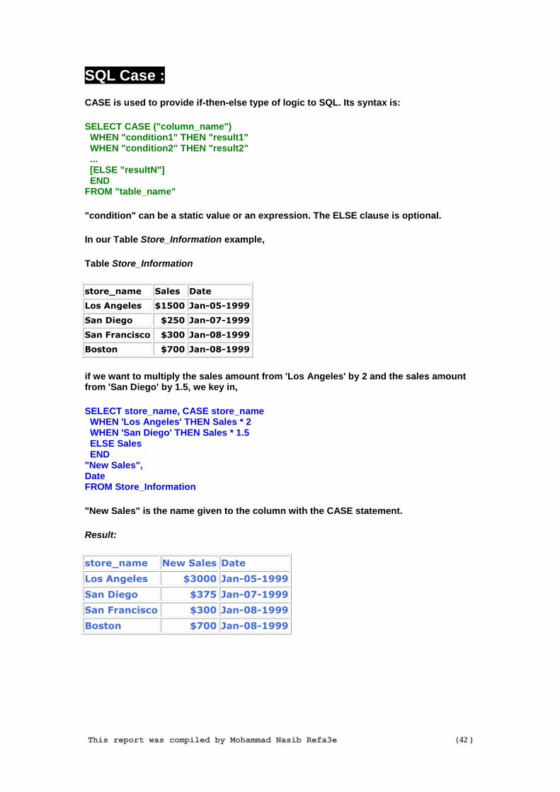
SQL Case :

CASE is used to provide if-then-else type of logic to SQL. Its syntax is:

SELECT CASE ("column_name") WHEN "condition1" THEN "result1" WHEN "condition2" THEN "result2" ... [ELSE "resultN"] END FROM "table_name"

"condition" can be a static value or an expression. The ELSE clause is optional.

In our Table Store_Information example,






Boston $700 Jan-08-1999

if we want to multiply the sales amount from 'Los Angeles' by 2 and the sales amount from 'San Diego' by 1.5, we key in,

SELECT store_name, CASE store_name WHEN 'Los Angeles' THEN Sales * 2 WHEN 'San Diego' THEN Sales * 1.5 ELSE Sales END "New Sales", Date FROM Store_Information

"New Sales" is the name given to the column with the CASE statement.

Result:

store_name New Sales Date




Boston $700 Jan-08-1999


SQL NULL :

In SQL, NULL means that data does not exist. NULL does not equal to 0 or an empty string. Both 0 and empty string represent a value, while NULL has no value.

Any mathematical operations performed on NULL will result in NULL. For example,

10 + NULL = NULL

Aggregate functions such as SUM, COUNT, AVG, MAX, and MIN exclude NULL values. This is not likely to cause any issues for SUM, MAX, and MIN. However, this can lead to confusion with AVG and COUNT.

Let's take a look at the following example:

Table Sales_Data

store_name Sales

Store A 300

Store B 200

Store C 100

Store D NULL

Below are the results for each aggregate function:

SUM (Sales) = 600

AVG (Sales) = 200

MAX (Sales) = 300

MIN (Sales) = 100

COUNT (Sales) = 3

Note that the AVG function counts only 3 rows (the NULL row is excluded), so the average is 600 / 3 = 200, not 600 / 4 = 150. The COUNT function also ignores the NULL rolw, which is why COUNT (Sales) = 3.

SQL ISNULL Function :

The ISNULL function is available in both SQL Server and MySQL. However, their uses are different:

SQL Server

In SQL Server, the ISNULL() function is used to replace NULL value with another value.


For example, if we have the following table,

Table Sales_Data

store_name Sales

Store A 300

Store B NULL

The following SQL,

SELECT SUM(ISNULL(Sales,100)) FROM Sales_Data;

returns 400. This is because NULL has been replaced by 100 via the ISNULL function.

MySQL

In MySQL, the ISNULL() function is used to test whether an expression is NULL. If the expression is NULL, this function returns 1. Otherwise, this function returns 0.

For example,

ISNULL(3*3) returns 0

ISNULL(3/0) returns

SQL IFNULL Function :

The IFNULL() function is available in MySQL, and not in SQL Server or Oracle. This function takes two arguments. If the first argument is not NULL, the function returns the first argument. Otherwise, the second argument is returned. This function is commonly used to replace NULL value with another value. It is similar to the NVL function in Oracle and the ISNULL Function in SQL Server.


Table Sales_Data

store_name Sales

Store A 300

Store B NULL

The following SQL,

SELECT SUM(IFNULL(Sales,100)) FROM Sales_Data;

returns 400. This is because NULL has been replaced by 100 via the ISNULL function.





SQL NVL Function :

The NVL() function is available in Oracle, and not in MySQL or SQL Server. This function is used to replace NULL value with another value. It is similar to the IFNULL Function in MySQL and the ISNULL Function in SQL Server.


Table Sales_Data

store_name Sales

Store A 300

Store B NULL

Store C 150

The following SQL,

SELECT SUM(NVL(Sales,100)) FROM Sales_Data;

returns 550. This is because NULL has been replaced by 100 via the ISNULL function, hence the sum of the 3 rows is 300 + 100 + 150 = 550.

SQL Coalesce Function ;

The COALESCE function in SQL returns the first non-NULL expression among its arguments.

It is the same as the following CASE statement:

SELECT CASE ("column_name") WHEN "expression 1 is not NULL" THEN "expression 1" WHEN "expression 2 is not NULL" THEN "expression 2" ... [ELSE "NULL"] END FROM "table_name"

For examples, say we have the following table,

Table Contact_Info

Name Business_Phone Cell_Phone Home_Phone

Jeff 531-2531 622-7813 565-9901

Laura NULL 772-5588 312-4088

Peter NULL NULL 594-7477

and we want to find out the best way to contact each person according to the following rules:

1. If a person has a business phone, use the business phone number.






2. If a person does not have a business phone and has a cell phone, use the cell phone number.

3. If a person does not have a business phone, does not have a cell phone, and has a home phone, use the home phone number.

We can use the COALESCE function to achieve our goal:

SELECT Name, COALESCE(Business_Phone, Cell_Phone, Home_Phone) Contact_Phone FROM Contact_Info;

Result:

Name Contact_Phone

Jeff 531-2531

Laura 772-5588

Peter 594-7477

SQL NULLIF Function ;

The NULLIF function takes two arguments. If the two arguments are equal, then NULL is returned. Otherwise, the first argument is returned.

It is the same as the following CASE statement:

SELECT CASE ("column_name") WHEN "expression 1 = expression 2 " THEN "NULL" [ELSE "expression 1"] END FROM "table_name"

For example, let's say we have a table that tracks actual sales and sales goal as below: Table Sales_Data

Store_name Actual Goal

Store A 50 50

Store B 40 50

Store C 25 30

We want to show NULL if actual sales is equal to sales goal, and show actual sales if the two are different. To do this, we issue the following SQL statement:

SELECT Store_name, NULLIF(Actual,Goal) FROM Sales_Data;

The result is:

Store_name NULLIF(Actual,Goal)

Store A NULL

Store B 40

Store C 25



SQL Rank :

Displaying the rank associated with each row is a common request, and there is no straightforward way to do so in SQL. To display rank in SQL, the idea is to do a self-join, list out the results in order, and do a count on the number of records that's listed ahead of (and including) the record of interest. Let's use an example to illustrate. Say we have the following table,

Table Total_Sales

Name Sales

John 10

Jennifer 15

Stella 20

Sophia 40

Greg 50

Jeff 20

we would type,

SELECT a1.Name, a1.Sales, COUNT(a2.sales) Sales_Rank FROM Total_Sales a1, Total_Sales a2 WHERE a1.Sales <= a2.Sales or (a1.Sales=a2.Sales and a1.Name = a2.Name) GROUP BY a1.Name, a1.Sales ORDER BY a1.Sales DESC, a1.Name DESC;

Result:

Name Sales Sales_Rank

Greg 50 1

Sophia 40 2

Stella 20 3

Jeff 20 3

Jennifer 15 5

John 10 6

Let's focus on the WHERE clause. The first part of the clause, (a1.Sales <= a2.Sales), makes sure we are only counting the number of occurrences where the value in the Sales column is less than or equal to itself. If there are no duplicate values in the Sales column, this portion of the WHERE clause by itself would be sufficient to generate the correct ranking.

The second part of the clause, (a1.Sales=a2.Sales and a1.Name = a2.Name), ensures that when there are duplicate values in the Sales column, each one would get the correct rank.


SQL Median :

To get the median, we need to be able to accomplish the following:

Sort the rows in order and find the rank for each row.

Determine what is the "middle" rank. For example, if there are 9 rows, the middle rank would be 5.

Obtain the value for the middle-ranked row.

Let's use an example to illustrate. Say we have the following table,

Table Total_Sales

Name Sales

John 10

Jennifer 15

Stella 20

Sophia 40

Greg 50

Jeff 20

we would type,

SELECT Sales Median FROM (SELECT a1.Name, a1.Sales, COUNT(a1.Sales) Rank FROM Total_Sales a1, Total_Sales a2 WHERE a1.Sales < a2.Sales OR (a1.Sales=a2.Sales AND a1.Name <= a2.Name) group by a1.Name, a1.Sales order by a1.Sales desc) a3 WHERE Rank = (SELECT (COUNT(*)+1) DIV 2 FROM Total_Sales);

Result:

Median

20

You will find that Lines 2-6 are the same as how we find the rank of each row. Line 7 finds the "middle" rank. DIV is the way to find the quotient in MySQL, the exact way to obtain the quotient may be different with other databases. Finally, Line 1 obtains the value for the middle-ranked row.

SQL Running Totals :

Displaying running totals is a common request, and there is no straightforward way to do so in SQL. The idea for using SQL to display running totals similar to that for displaying rank: first do a self-join, then, list out the results in order. Where as finding the rank requires doing a count on the number of records that's listed ahead of (and including) the record of interest, finding the running total requires summing the values for the records that's listed ahead of (and including) the record of interest.

http://www.1keydata.com/sql/sql-rank.html


Let's use an example to illustrate. Say we have the following table,

Table Total_Sales

Name Sales

John 10

Jennifer 15

Stella 20

Sophia 40

Greg 50

Jeff 20

we would type,

SELECT a1.Name, a1.Sales, SUM(a2.Sales) Running_Total FROM Total_Sales a1, Total_Sales a2 WHERE a1.Sales <= a2.sales or (a1.Sales=a2.Sales and a1.Name = a2.Name) GROUP BY a1.Name, a1.Sales ORDER BY a1.Sales DESC, a1.Name DESC;

Result:

Name Sales Running_Total

Greg 50 50

Sophia 40 90

Stella 20 110

Jeff 20 130

Jennifer 15 145

John 10 155

The combination of the WHERE clause and the ORDER BY clause ensure that the proper running totals are tabulated when there are duplicate values.

SQL Percent To Total :

To display percent to total in SQL, we want to leverage the ideas we used for rank/running total plus subquery. Different from what we saw in the SQL Subquery section, here we want to use the subquery as part of the SELECT. Let's use an example to illustrate. Say we have the following table,

Table Total_Sales

Name Sales

John 10

Jennifer 15

Stella 20

Sophia 40

Greg 50

Jeff 20

http://www.1keydata.com/sql/sql-subquery.html


we would type,

SELECT a1.Name, a1.Sales, a1.Sales/(SELECT SUM(Sales) FROM Total_Sales) Pct_To_Total FROM Total_Sales a1, Total_Sales a2 WHERE a1.Sales <= a2.sales or (a1.Sales=a2.Sales and a1.Name = a2.Name) GROUP BY a1.Name, a1.Sales ORDER BY a1.Sales DESC, a1.Name DESC;

Result:

Name Sales Pct_To_Total

Greg 50 0.3226

Sophia 40 0.2581

Stella 20 0.1290

Jeff 20 0.1290

Jennifer 15 0.0968

John 10 0.0645

The subquery "SELECT SUM(Sales) FROM Total_Sales" calculates the sum. We can then divide the individual values by this sum to obtain the percent to total for each row.

SQL Cumulative Percent To Total :

To display cumulative percent to total in SQL, we use the same idea as we saw in the Percent To Total section. The difference is that we want the cumulative percent to total, not the percentage contribution of each individual row. Let's use the following example to illuatrate: Table Total_Sales

Name Sales

John 10

Jennifer 15

Stella 20

Sophia 40

Greg 50

Jeff 20

http://www.1keydata.com/sql/sql-percent-to-total.html


we would type, SELECT a1.Name, a1.Sales, SUM(a2.Sales)/(SELECT SUM(Sales) FROM Total_Sales) Pct_To_Total FROM Total_Sales a1, Total_Sales a2 WHERE a1.Sales <= a2.sales or (a1.Sales=a2.Sales and a1.Name = a2.Name) GROUP BY a1.Name, a1.Sales ORDER BY a1.Sales DESC, a1.Name DESC;

Result:

Name Sales Pct_To_Total

Greg 50 0.3226

Sophia 40 0.5806

Stella 20 0.7097

Jeff 20 0.8387

Jennifer 15 0.9355

John 10 1.0000

The subquery "SELECT SUM(Sales) FROM Total_Sales" calculates the sum. We can then divide the running total, "SUM(a2.Sales)", by this sum to obtain the cumulative percent to total for each row.

اخلامتة

امكتابلك من اهتفع هبدى اىل

لك مسمل ومسلمة اىل

هللا محمد رسول لك من يشهد ان ال اهل الا هللا اىل

يمنيب الاوملن يصًل عىل ام ادلعا يل أ رجو

هلل رب امعاملني وامحلد

sql command

Technology