spurious solutions for transient maxwell equations … zurich¨ spurious solutions for transient...

ETH ZURICH

Spurious Solutions for transientMaxwell equations in 2D

Semester Work

presented by:

Andres Rosero

Born 8 November 1978

citizen of Ambato, Ecuador

Supervision:

Prof. Ralf Hiptmair

April 8, 2011

Contents

I Abbreviations 3

1 Introduction 4

2 Theoretical aspects 6

2.1 Boundary Value Problem . . . . . . . . . . . . . . . . . . . . 6

2.2 Finite Elements . . . . . . . . . . . . . . . . . . . . . . . . . . 8

2.3 Regularization . . . . . . . . . . . . . . . . . . . . . . . . . . 10

2.3.1 grad-div Regularization . . . . . . . . . . . . . . . . . 11

2.3.2 Discrete Regularization . . . . . . . . . . . . . . . . . 12

2.4 Time stepping . . . . . . . . . . . . . . . . . . . . . . . . . . . 13

3 Implementation 15

3.1 Code . . . . . . . . . . . . . . . . . . . . . . . . . . . . . . . . 15

3.1.1 Main Routines . . . . . . . . . . . . . . . . . . . . . . 16

3.1.1.1 run.m . . . . . . . . . . . . . . . . . . . . . . 16

3.1.1.2 leapfrog.m . . . . . . . . . . . . . . . . . . 18

3.1.1.3 assemMat LFE.m . . . . . . . . . . . . . . . . 23

3.1.1.4 MASSLump LFE.m . . . . . . . . . . . . . . . 25

3.1.1.5 P7O6.m . . . . . . . . . . . . . . . . . . . . . 25

3.1.1.6 shap W1F.m . . . . . . . . . . . . . . . . . . 26

3.1.1.7 assemMat W1F.m . . . . . . . . . . . . . . . . 27

3.1.1.8 MASSW1F.m . . . . . . . . . . . . . . . . . . 29

3.1.1.9 STIMA Curl W1F.m. . . . . . . . . . . . . . . 30

3.1.1.10 assemMat WRegW1F2.m . . . . . . . . . . . . 31

3.1.1.11 grad shap LFE.m . . . . . . . . . . . . . . . 33

3.1.1.12 STIMA WRegW1Fb.m . . . . . . . . . . . . . . 34

3.1.1.13 assemLoad W1F.m . . . . . . . . . . . . . . . 35

1

3.1.1.14 shap LFE2.m . . . . . . . . . . . . . . . . . . 37

3.1.1.15 assemMat LFE3.m . . . . . . . . . . . . . . . 37

3.1.1.16 MASSLFE2.m . . . . . . . . . . . . . . . . . . 39

3.1.1.17 STIMA Curl LFE2.m . . . . . . . . . . . . . . 40

3.1.1.18 STIMA Reg LFE2.m . . . . . . . . . . . . . . . 41

3.1.1.19 assemLoad LFE3.m . . . . . . . . . . . . . . 41

3.2 Initial Value . . . . . . . . . . . . . . . . . . . . . . . . . . . . 43

3.2.0.20 initL.m . . . . . . . . . . . . . . . . . . . . 43

3.2.0.21 initSq.m . . . . . . . . . . . . . . . . . . . . 44

3.2.1 Plotting . . . . . . . . . . . . . . . . . . . . . . . . . . 45

3.2.1.1 plotfield1.m . . . . . . . . . . . . . . . . . 45

3.2.1.2 plotiterate1.m . . . . . . . . . . . . . . . 45

3.2.1.3 plot LFE.m . . . . . . . . . . . . . . . . . . 46

3.2.1.4 plot Mesh.m . . . . . . . . . . . . . . . . . . 48

3.2.1.5 plot Norm W1F.m . . . . . . . . . . . . . . . 53

3.2.2 Mesh . . . . . . . . . . . . . . . . . . . . . . . . . . . . 55

3.2.2.1 sqr str gen.m . . . . . . . . . . . . . . . . . 55

3.2.2.2 Lshap str gen.m . . . . . . . . . . . . . . . 56

3.2.2.3 load Mesh.m . . . . . . . . . . . . . . . . . . 57

3.2.2.4 refine REG.m . . . . . . . . . . . . . . . . . 58

3.2.3 Viewing results . . . . . . . . . . . . . . . . . . . . . . 65

3.2.3.1 replay.m . . . . . . . . . . . . . . . . . . . . 65

4 Numerical Experiments 69

4.1 Domain . . . . . . . . . . . . . . . . . . . . . . . . . . . . . . 69

4.2 Starting Conditions . . . . . . . . . . . . . . . . . . . . . . . . 70

4.2.1 Singular Starting Conditions . . . . . . . . . . . . . . 70

4.2.2 Smooth Starting Conditions . . . . . . . . . . . . . . . 71

4.3 Time Stepping . . . . . . . . . . . . . . . . . . . . . . . . . . 72

4.4 Results . . . . . . . . . . . . . . . . . . . . . . . . . . . . . . . 73

4.4.1 Energy Behaviour Using a Singular Initial Function . 74

4.4.2 Energy Behaviour Using a Smooth Initial Function . . 76

4.4.3 Convergence results . . . . . . . . . . . . . . . . . . . 78

2

Chapter I

Abbreviations

Ch. ChapterFEM Finite elements methodsPDE Partial differential equationp. PageODE Ordinary differential equationTh. Theoremrhs. Right hand sidew.r.t. With respect to

3

Chapter 1

Introduction

Electromagnetic phenomena is well described by the Maxwell Equations

divD = ρ

divB = 0

curlE = − ddtB (1.1)

curlH = ddtD+ J (1.2)

and B = µH, D = ǫE, where E and B are the electric and the magneticfield, ρ is the total charge density and J the total current density.The first two equations describe how the sources generate the fields, whereasthe last two describe the time evolution of the fields.

Numerical solutions to these equations can be found using FEM, however theinappropriate application of FEM could generate spurious solutions. Thesesolutions are not physical, i.e. can not be observed in reality [1, p.323], [2].

This work illustrates and compares spurious solutions obtained using Nodalelements with the right solutions obtained using edge elements for transientMaxwell’s equations in a 2D-domain.

In Chapter 2, we present the Cauchy problem and state its variational for-mulation. We also describe the application of FEM for nodal and edgeelements furthermore we give some stability conditions to ensure the rightchoice for the time-step.

Chapter 3 illustrates the MATLAB implementation with the correspondingcomments and discusses some difference between the two discretizations.Finally in Chapter 4 we describe numerical experiments carried on on a

4

square and on an L-shaped domain and compare the results for the nodaland edge elements andfor different mesh-sizes.

The structure of this work is based on [3], however there are some partsthat were quoted literally from [3] as we were not able to find an equivalentformulation.

5

Chapter 2

Theoretical aspects

Equation (1.1) is called Faraday law and describes how changes of the Mag-netic field, induce an electric field. Equation (1.2) is called Ampere’s lawand describes how current flux and changes in the electrical field generatea magnetic field. To decouple this two equations we can apply the curloperator on (1.1)

curl curlE = − ddtcurlB.

Let us assume that J is constant and insert (1.2) in the right hand side (rhs),so we obtain the electric wave equation

curl curlE = − d2

dt2E. (2.1)

The two dimensional version of (2.1) can be used to compute the electricalfield for translational symmetric systems. We consider numerical solutionsfor such version using FEM, on this purpose we start stating the Cauchyproblem.

2.1 Boundary Value Problem

The curl operator is defined for functions u ∈ C1(R3;R3). For our twodimensional problem we use the differential operators

curl2D u =(

−∂u∂y

∂u∂x

)T, for u ∈ C1(R2;R),

and

curl2D u =∂u1

∂y−∂u2

∂x, for u ∈ C1(R2;R2).

6

Then the electric field E(x, t) in homogeneous, isotropic materials solves theboundary value problem

d2

dt2E+ curl2D curl2D E = 0 in Ω× (0, T )

E(·, t)× n = 0 on ∂Ω × (0, T )E(x, 0) = E0 in ΩddtE(x, 0) = 0 in Ω,

(2.2)

where Ω ∈ R2 is a bounded domain, T ∈ R+ and E0 ∈ H0(curl; Ω) :=v ∈ L2(Ω) : curl2D v ∈ L2(Ω),v × n = 0

. Let us also assume divE0 = 0.

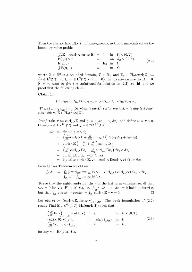
Now we want to give the variational formulation to (2.2), to this end weproof first the following claim.

Claim 1.

(curl2D curl2D E, v)L2(Ω) = (curl2D E, curl2D v)L2(Ω)

Where (u,v)L2(Ω) :=∫

Ω〈u,v〉dx is the L2-scalar product, v is any test func-tion with v, E ∈ H0(curl; Ω).

Proof. take ν := curl2D E and η := v1 dx1 + v2 dx2, and define ω = ν ∧ η.Clearly ν ∈ DF0,1(Ω) and η, ω ∈ DF1,1(Ω).

dω = dν ∧ η + ν ∧ dη

=(

∂∂x1

curl2D E+ ∂∂x2

curl2D E)

∧ (v1 dx1 + v2 dx2)

+ curl2D E(

− ∂∂v1

+ ∂∂v2

)

dx1 ∧ dx2

=(

∂∂x1

curl2D Ev2 −∂

∂x2curl2D Ev1

)

dx1 ∧ dx2

− curl2D Ecurl2D vdx1 ∧ dx2= (〈curl2D curl2D E,v〉 − curl2D Ecurl2D v) dx1 ∧ dx2.

From Stokes Theorem we obtain∫

Ω dω =∫

Ω (〈curl2D curl2D E,v〉 − curl2D Ecurl2D v) dx1 ∧ dx2=

∫

∂Ωω =

∫

∂Ωcurl2D E ∧ v.

To see that the right-hand-side (rhs.) of the last term vanishes, recall thatγtv = 0 for v ∈ H0(curl; Ω), i.e.

∫

∂Ωv1 dx1 + v2 dx2 = 0 holds pointwise,

but then∫

∂Ωνv1dx1 + νv2dx2 =

∫

∂Ωcurl2D E ∧ v = 0

Let a(u, v) := (curl2D E, curl2D v)L2(Ω). The weak formulation of (2.2)

reads: Find E ∈ C2([0;T ],H0(curl; Ω)) such that(

d2

dt2E,v

)

L2(Ω)+ a(E,v) = 0 in Ω× (0, T )

(Eh(x, 0),v)L2(Ω) = (E0,v)L2(Ω) in Ω(∂∂tEh(x, 0),v

)

L2(Ω)= 0 in Ω ,

(2.3)

for any v ∈ H0(curl; Ω).

7

Remark 1. Note that the operator a(·, ·) is symmetric and satisfies an ellip-tical condition (it follows immediately from the Friedrichs Inequality). Thisfact implies the existence end uniqueness of Weak solutions of (2.3). Weaksolutions can be approximated using FEM. In the next section we describethe application of this method.

2.2 Finite Elements

In this section we want to give a detailed procedure to approximate (2.3)using FEM. The starting point of every FE-algorithm is the discretizationof the domain Ω. We choose a triangular mesh Th = TiN , where Ti :=(ai1,a

i2,a

i3) is the i-th triangle with vertices aij ∈ Ω, j = 1, 2, 3, h is the mesh

width, and N(h) := |Th|.

Let Vh ∈ H0(curl; Ω) be a finite dimensional linear subspace with ba-

sis wiN . We define the FE-approximation Eh =N∑

i=1

Ei(t)wi(x) to E ∈

C2([0;T ],H0(curl; Ω)) by: Find Eh ∈ Vh such that(

d2

dt2Eh,v

)

L2(Ω)+ a(Eh,v) = 0 in Ω× (0, T )


)

L2(Ω)= 0 in Ω ,

(2.4)

for any v ∈ Vh. Expanding Eh and v on its basis functions we obtain

N∑

i=1

d2

dt2Ei(t)wi(x),

N∑

j=1

vjwj(x)

L2(Ω)

+ a

N∑

i=1

Ei(t)wi(x),N∑

j=1

vjwj(x)

=

N∑

i=1

N∑

j=1

vj (wi(x), wj(x))L2(Ω)d2

dt2Ei(t) +

N∑

i=1

N∑

j=1

vj a (wi(x), wj(x))Ei(t) .

We can write this expression using matrices as

~vtM~E+ ~vtC~E = 0

where ~E := EiN , ~v := vjN , Mij := (wi, wj)L2(Ω) and Cij := a(wi, wj).

Finally the ODE corresponding to (2.4) reads

M~E+ C~E = 0

~E0 = 0~E0 = ΠVh

E0

(2.5)

This linear system has a leak, it will not ensure divE(·, t) = 0 for all times.Regularization terms will solve the problem. This will be discussed in the

8

next section. Now, before we take a closer look in the FE-spaces Vh, wedescribe the FE-algorithm, which is mainly based on

• a reference element T

• an element mapping FT : T → T ∈ Th

• reference shape-functions N,

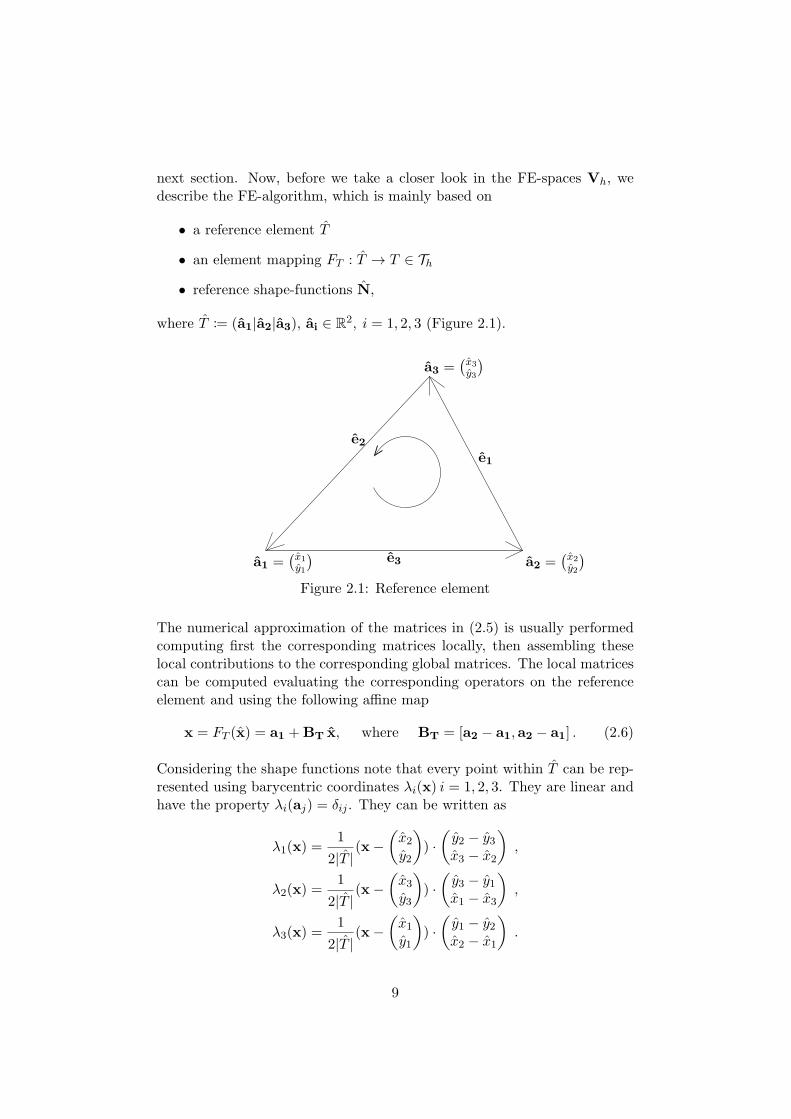
where T := (a1|a2|a3), ai ∈ R2, i = 1, 2, 3 (Figure 2.1).

a1 =(x1

y1

)a2 =

(x2

y2

)

a3 =(x3

y3

)

e1

e2

e3

Figure 2.1: Reference element

The numerical approximation of the matrices in (2.5) is usually performedcomputing first the corresponding matrices locally, then assembling theselocal contributions to the corresponding global matrices. The local matricescan be computed evaluating the corresponding operators on the referenceelement and using the following affine map

x = FT (x) = a1 +BT x, where BT = [a2 − a1,a2 − a1] . (2.6)

Considering the shape functions note that every point within T can be rep-resented using barycentric coordinates λi(x) i = 1, 2, 3. They are linear andhave the property λi(aj) = δij . They can be written as

λ1(x) =1

2|T |(x−

(x2y2

)

) ·

(y2 − y3x3 − x2

)

,

λ2(x) =1

2|T |(x−

(x3y3

)

) ·

(y3 − y1x1 − x3

)

,

λ3(x) =1

2|T |(x−

(x1y1

)

) ·

(y1 − y2x2 − x1

)

.

9

Their gradients are constant and read

gradλ1 = 12|T |

(y2 − y3x3 − x2

)

,

gradλ2 = 12|T |

(y3 − y1x1 − x3

)

,

gradλ3 = 12|T |

(y1 − y2x2 − x1

)

,

(2.7)

where |T | denotes the area of T .We will use the following FE-spaces

• Sh := v ∈ C0(Ω) ∩H10 (Ω), v|T ∈ P1(T ) ∀T ∈ Th ,

with local basis BST= λ1, λ2, λ3 ,

• Nh := v ∈ (C0(Ω))2 ∩H0(curl; Ω), v|T ∈ (P1(T ))2 ∀T ∈ Th

with local basis BNT=(

λ1

0

),(0λ1

),(λ2

0

),(0λ2

),(λ3

0

),(0λ3

)

• Eh := lowest order Whitney 1-forms ⊂ H0(curl; Ω) ,

with local basis BET=

λ2gradλ3 − λ3gradλ2,λ3gradλ1 − λ1gradλ3,λ1gradλ2 − λ2gradλ1

The Edge elements are a very powerful tool to discretize Maxwell’s equa-tions. The reason is that they present the same properties in discrete spacesas differential forms have in continuous spaces. Let for example ei be theedge of T opposite to ai and directed as shown in Figure 2.1, furthermorelet φj ∈ BE

T, then the local edge elements satisfy

1

|T |

∫

T

curl2D φidx =︸︷︷︸

Gauss

−1

|T |

∫

∂T

φid~s = −1

|T |

3∑

j=1

∫

ej

φid~s

︸︷︷︸

δij

= −1

|T |,

i.e. the curl2D of these vector fields are constant on T . This fact will beuseful for the generation of the local curl Matrix. Another property of edgeelements is useful for the regularization of (2.4), it is described next.

2.3 Regularization

The FE-discretization (2.4) may produce approximations to non-physicalsolutions, the so-called spurious solutions. The reason lays in the kernelof the operator a(·, ·) [1, p. 318, Ch. 6], [2]. Recall that in (2.2) we re-quired divE0 = 0, theoretically this conditions ensures that E(·, t) behaves

10

divergence-free for all t ∈ [0, T ]. Unfortunately, “a slight perturbation ofthe initial value might lead to growing curl2D -free components in E(., t)that may eventually swamp the physically meaningful solution. A remedyis offered by regularization”1.

2.3.1 grad-div Regularization

Consider the electric Maxwell’s eigenvalue problem

(curl2D E, curl2D v)L2(Ω) = ω2 (E,v)L2(Ω) , ∀v ∈ H0(curl; Ω).

It can be proven ([1, Ch. 4]) that the solution

E ∈ Z0(I,Ω) :=

u ∈ H0(curl; Ω)∣∣∣(u,Z)L2(Ω) = 0, ∀z ∈ H0(curl0; Ω)

. The

reason why this is relevant for the continuous regularization is to be clarifiedwith the next claim.

Claim 2. E ∈ Z0(I,Ω) ⇒ divE = 0

Proof. From Poincare’s theorem we know that a 0-form νz exist, s.t.ωz = dνz, where ωu := u1dx1 + u2dx2 is the 1-form induced by the vectorfield u ∈ C(Ω;R2).Let ξ := ν ∧ ∗ωE then

∫

Ω

dξ =

∫

Ω

dνz ∧ ∗ωE

︸︷︷︸

=(E,z)L2(Ω)=0

+

∫

Ω

νz ∧ d ∗ ωE

︸︷︷︸∫

Ω

νzdivEdx

=︸︷︷︸

stoke’s Thm.

∫

∂Ω

νz ∧ ∗ωE.

A test function z s.t. νz ∈ H10 (Ω) yields the result.

Our goal is to state a variational problem equivalent to (2.3). Using the lastclaim we end up with: seek E ∈ C2([0;T ],H0(curl; Ω) ∩ H(div; Ω)) suchthat for all v ∈ H0(curl; Ω) ∩H(div; Ω)(

d2

dt2E,v

)

L2(Ω)+ a(E,v) + (divE, divv)L2(Ω) = 0 in Ω× (0, T )


)

L2(Ω)= 0 in Ω .

(2.8)

We will use Nh to discretize (2.8). Proceeding the same way as in (2.4) weend up with the following ODE

M ~E+ C~E+ R~E = 0

~E0 = 0~E0 = ΠVh

E0 ,

(2.9)

1Quoting from [3]

11

where R corresponds to the regularization term, C and M are the stiffnessand mass matrices. Here we denote with · a matrix w.r.t. Nh. Note that,since Nh ∈ H1(Ω), we are looking for a FE-approximation Eh ∈ H1

x :=H1(Ω) ∩ H0(curl; Ω). Unfortunately Eh does not always converge to E.This is the statement of the following theorem from [1, Ch 6, Thm. 6.3,p.322 ].

Theorem 1. The space H1x(Ω) is a closed subspace of X0(I,Ω) and the

inclusion is strict, if Ω has re-entrant edges or corners.

We will illustrate this phenomena with an example, where an electromag-netic field on a square domain and on an L-shaped domain is approximated.A comparison’s reference is delivered by edge elements using a discrete reg-ularization.

2.3.2 Discrete Regularization

The variational problem (2.8) can not be discretized with edge elementsbecause Eh * H(div ,Ω). The way out is to regularise (2.4), exploiting thefact that gradSh ⊂ Eh, we obtain

(Eh,grad vh)L2(Ω) = 0 ∀ vh ∈ Sh, (2.10)

for Eh ∈ Eh solving (2.4). The last expression holds in a discrete level, butsince Whitney forms behave as differential forms do on a continuous level,(2.10) can be justified, considering ω := v ∧ ∗E, and

∫

Ω

dω =

∫

Ω

dv ∧ ∗E

︸︷︷︸

=∫

Ω

〈grad v,E〉dx

+

∫

Ω

v ∧ d ∗E

︸︷︷︸

=∫

Ω

vdivEdx

Stokesthm.=

∫

∂Ω

ω

︸︷︷︸∫

∂Ω

v∧∗E

= 0 ∀v ∈ H10 (Ω).

The discrete regularised weak formulation reads: Find Eh ∈ C2([0, T ], Eh),such that(

d2

dt2Eh,v

)

L2(Ω)+ a(Eh,v) + (vh,grad ph)L2(Ω) = 0 in Ω× (0, T )

(Eh,grad qh)L2(Ω) − d(ph, qh) = 0 in Ω× (0, T )


)

L2(Ω)= 0 in Ω ,

(2.11)

for any vh ∈ Eh, qh ∈ Sh, where d(·, ·) is an arbitrary symmetric positivedefinite (spd) bilinear form on Sh as ph = 0 anyway. For numerical issues apractical choice is the lumped L2(Ω) inner product, since its corresponding

12

matrix is diagonal.Expanding Eh, vh on its respective basis functions, we obtain

(Eh,grad qh)L2(Ω) =

NE∑

i=1

Eih(t)w

Ei ,grad

NN∑

j=1

wSj

L2(Ω)

=

NE∑

i=1

NN∑

j=1

(wEi ,gradw

Nj

)

L2(Ω)︸︷︷︸

=:Gij

Eih(t).

The coupled ODE for (2.11) reads

M~E + C~E + G~p = 0

Gt~E − D~p = 0,

where D corresponding to d(·, ·) is diagonal, M and C are the mass and curlmatrices w.r.t Eh. Decoupling we obtain

M~E+ (C +GD−1Gt)~E = 0

~E0 = 0~E0 = ΠEhE0 .

(2.12)

In the next section we discuss a way to compute approximations to thesolutions of (2.12) and (2.9).

2.4 Time stepping

Clearly we are interested only in Runge-Kutta schemes conserving the totalenergy in the system. We choose the leapfrog scheme and apply it to (2.9),

~E0 = M−1ΠNhE0

~E1 = ~E0 − 1/2τ2M−1(C + R)~E0

~En+1 = 2~En − ~En−1 − τ2M−1(C + R)~En ,

(2.13)

where the condition ~E = 0 is interpreted as ~E1 = ~E−1 and used to obtain~E1.The starting condition for the Eh-discretization is a little more complicated,as we have to ensure that ~E0 is divergence-free on the discrete level, ie

(divE0

h, φh)

L2(Ω)=(E0

h,gradφh)

L2(Ω)= 0 ∀φh ∈ Sh. (2.14)

This condition is fulfilled, if we find E0h ∈ Nh, uh ∈ Nh for all vh,wh ∈ Nh

(E0

h,vh

)

L2(Ω)+ (curl2D uh, curl2D vh)L2(Ω) = (E0,vh)L2(Ω) ,

(curl2D E0

h, curl2D wh

)

L2(Ω)=

(curl2D E0, curl2D wh

)

L2(Ω).

13

Let Qh denote the L2(Ω)-orthogonal projection onto the space Th of piece-wise constant functions, and ΠEh the local edge elements interpolation op-erator, then the following diagram holds

curl2D ΠEh = Qh curl2D

Note that curl2D E0h = Qh(curl2D E0), i.e. curl2D (E0

h − ΠEHE0) = 0, thusexists φh ∈ S1 with E0

h −ΠEE0 = gradφh and satisfies

(gradφh,gradψh)L2(Ω) = (E0 −ΠhE0,gradψh)L2(Ω) = − (ΠhE0,gradψh)L2(Ω) .

Its matrix representation reads

GtMG~φ = GtMΠEh~E0

Substitution of ~φ in ~E0h − ΠEhE0 = G~φ yields the desired starting value.

Thus the ODE to be considered reads

~E0h = (I +G(GtMG)−1GtM)ΠEhE0

~E1 = ~E0 − 1/2τ2M−1(C +GD−1Gt)~E0

~En+1 = 2~En − ~En−1 − τ2M−1(C +GD−1Gt)~En .

(2.15)

A CFL condition∥∥∥1/2τ2M−1(C + R)

∥∥∥ ≤ 1 for (2.13), and

∥∥1/2τ2M−1(C +GD−1Gt)

∥∥ ≤ 1 for (2.15)

ensures the stability of the scheme as time evolves. An accurate estimationof the time step τ requires the computation of the largest eigenvalue of thecorresponding operators. In our simulation we only ensure that the CFLcondition is fulfilled, thus we just choose τ = Ch, where h is the mesh widthand the constant 0 ≤ C ∈ R small enough. Our implementation computesapproximations to the solutions of (2.13) and (2.15). We give in the nextchapter some details of the structure of the program.

14

Chapter 3

Implementation

In this chapter we present the implementation of a program computing ap-proximations to the solutions for transient Maxwell’s equations using FEM.The program was done in MATLAB using the “LehrFem” framework, somost of the code was already available. Very useful was the code of Prof.Hiptmair, the structure of the main function is actually based on this code.

The program is structured as shown in Figure 3.1. The starting point isthe routine run.m . It computes and plots the electrical field ~E, and plotsalso the total energy, for both (2.12) and (2.9), giving a singular functionas starting value E0, for an square mesh width an initial mesh width h0and initial time step τ0 = 0.01. The representation of the plots allowsan easy comparison between the two discretizations. The final time is setto T = 3. A plot of the time evolution of the magnetic and electricalenergy is displayed when T is reached. The same is performed for an L-shaped mesh. This process is repeated “NREFS= 5” times, refining ineach step the mesh by hn+1 = hn/2. The routine run smooth.m performsthe equivalent simulation, but for smooth starting conditions. More detailsabout the numerical experiments are given in Chapter 4.

3.1 Code

In this section we list almost all the code. Some less important routines arenot included, even though there is quite a lot of code. For this reason wehave divided the routines in five groups. In the first group we have listedthe most important functions, i.e the functions needed to compute (2.12)and (2.9). The second group contains the routines implementig the startingfunctions, the next section lists the routines used to plot the results, followedby the routines used for meshing and finally we list the routine used to plotthe computed results again saving the ploted results in avi-files.

15

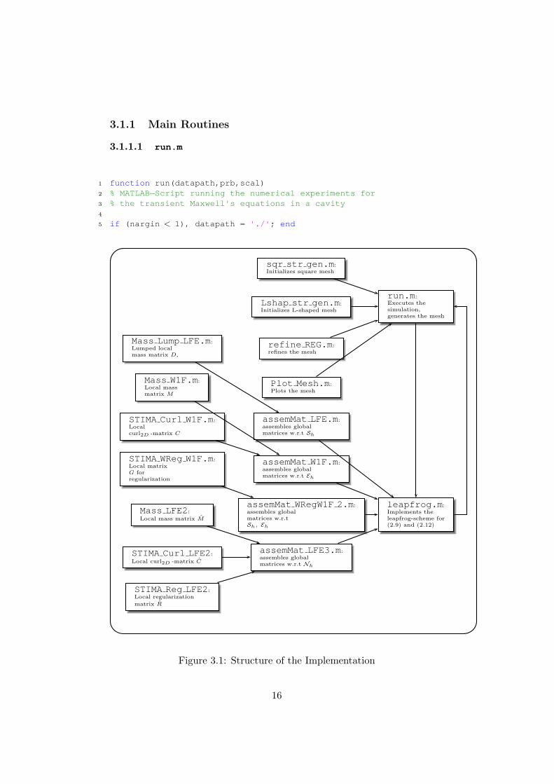
3.1.1 Main Routines

3.1.1.1 run.m

1 function run(datapath,prb,scal)2 % MATLAB−Script running the numerical experiments for3 % the transient Maxwell's equations in a cavity4

5 if (nargin < 1), datapath = './' ; end

sqr str gen.m :Initializes square mesh

Lshap str gen.m :Initializes L-shaped mesh

run.m :Executes thesimulation,generates the mesh

Mass Lump LFE.m:Lumped localmass matrix D,

refine REG.m:refines the mesh

Mass W1F.m:Local massmatrix M

Plot Mesh.m:Plots the mesh

STIMA Curl W1F.m:Localcurl2D -matrix C

assemMat LFE.m:assembles globalmatrices w.r.t Sh

STIMA WRegW1F.m:Local matrixG forregularization

assemMat W1F.m:assembles globalmatrices w.r.t Eh

Mass LFE2:

Local mass matrix M

assemMat WRegW1F2.m :assembles globalmatrices w.r.tSh, Eh

leapfrog.m :Implements theleapfrog-scheme for(2.9) and (2.12)

STIMA Curl LFE2:

Local curl2D -matrix C

assemMat LFE3.m :assembles globalmatrices w.r.t Nh

STIMA Reg LFE2:Local regularization

matrix R

Figure 3.1: Structure of the Implementation

16

6 if (nargin < 2), prb = −1; end7 if (nargin < 3), scal = 0.5; end8

9 % Initialize constants10

11 InitREF = 2; % size of the Initial Mesh12 NREFSs = 5; % Number of unifrom mesh refinements13 finaltime = 3;14 timestep = 0.01;15

16 disp( 'MATLAB based numerical experiments for transient Maxwell equations' );17 disp( 'Goal is the comparison of nodal and edge element discretiza tions' );18 fprintf( 'Path for output files %s \n' ,datapath);19 fprintf( 'Relative scaling of C and R: %d <−> %d\n' ,2 * scal,2 * (1 −scal));20

21 % Generate initial meshes, where the meshwidth depends on In itREF22 %Square mesh23 MeshS=sqr str gen(InitREF);24 %Add to the mesh some useful information to handle edge eleme nts25 MeshS.ElemFlag = ones(size(MeshS.Elements,1),1);26 MeshS = add Edges(MeshS);27 LocS = get BdEdges(MeshS);28 MeshS.BdFlags = zeros(size(MeshS.Edges,1),1);29 MeshS.BdFlags(LocS) = −1;30

31 %L−shaped mesh32 MeshL=Lshap str gen(InitREF);33 %Add to the mesh some useful information to handle edge eleme nts34 MeshL.ElemFlag = ones(size(MeshL.Elements,1),1);35 MeshL = add Edges(MeshL);36 LocL = get BdEdges(MeshL);37 MeshL.BdFlags = zeros(size(MeshL.Edges,1),1);38 MeshL.BdFlags(LocL) = −1;39

40 % Do NREFS uniform refinement steps41

42 for i = 1:NREFSs43

44 % For the square mesh45 % Refine Mesh46 MeshS = refine REG(MeshS);47 % plot it48 plot Mesh(MeshS, 'as' )49

50 % start leapfrog with starting condition initSq51 [en,sol v,sol e,times] = leapfrog(MeshS,@initSq,timestep * (2ˆ( −i+1)),finaltime,2ˆ(i −1)52

53 %Saving Data54 Sq str=[ 'Square' int2str(i)];55 fprintf([ 'Finished on' Sq str ': Results stored in %s' ],[datapath,[Sq str, ' res' ]]);56 save([datapath, Sq str, ' res' ], 'en' , 'sol v' , 'sol e' , 'times' );57

58 %plot energy evolution in time59 figure; clf;

17

60 subplot(1,2,1);61 plot(en(:,1),en(:,2), 'r −' ,en(:,1),en(:,4), 'b −' );62 legend( 'Nodal scheme' , 'Edge elements' );63 title([Sq str, ': Electric energy' ]);64 xlabel( 'time' );65 subplot(1,2,2);66 plot(en(:,1),en(:,3), 'r −' ,en(:,1),en(:,5), 'b −' );67 legend( 'Nodal scheme' , 'Edge elements' );68 title([Sq str, ': Magnetic energy' ]);69 xlabel( 'time' );70 drawnow;71 clear en solv sole times;72 % end for the square mesh73

74

75 %For the L −mesh76 % Refine mesh77 MeshL = refine REG(MeshL);78 plot Mesh(MeshL, 'as' )79

80 % start leapfrog with starting condition initL81 [en,sol v,sol e,times] = leapfrog(MeshL,@initL,timestep * (2ˆ( −i+1)),finaltime,2ˆ(i −1),82

83 %Saving Data84 L str=[ 'Lshape' int2str(i)];85 fprintf([ 'Finished on' L str ': Results stored in %s' ],[datapath,[L str, ' res' ]]);86 save([datapath, L str, ' res' ], 'en' , 'sol v' , 'sol e' , 'times' );87

88 % Actualize energy plot89 figure; clf;90 subplot(1,2,1);91 plot(en(:,1),en(:,2), 'r −' ,en(:,1),en(:,4), 'b −' );92 legend( 'Nodal scheme' , 'Edge elements' );93 title([L str, ': Electric energy' ]);94 xlabel( 'time' );95 subplot(1,2,2);96 plot(en(:,1),en(:,3), 'r −' ,en(:,1),en(:,5), 'b −' );97 legend( 'Nodal scheme' , 'Edge elements' );98 title([L str, ': Magnetic energy' ]);99 xlabel( 'time' );

100 drawnow;101 clear en solv sole times;102

103

104 end

3.1.1.2 leapfrog.m

1 function [energies,sol v,sol e,times] = leapfrog(Mesh,init field,ts,T,grabstep,scal)2 % leapfrog timestepping discretizations of Maxwell's equa tions3 %4 % Mesh −> 2D unstructured mesh

18

5 % init field −> string designating the routine providing the initial6 % vectorfield7 % ts −> timestep8 % T −> final time9 % grabstep −> every #grabstep iterate will be sampled

10 % scal −> governs strength of regularization11 % A = 2* (scal * C + (1−scal) * R)12 %13 % Result:14 %15 % energies −> trace of electric/magnetic energies during timestepping16 % energies(:,1) = time,17 % energies(:,2) = electric energy of nodal solution18 % energies(:,3) = magnetic energy of nodal solution19 % energies(:,4) = electric energy of edge element solution20 % energies(:,5) = magnetic energy of edge element solution21 % sol v −> sampled solutions for nodal FEM22 % sol e −> sampled solutions for edge elements23 % times −> vector of sampling times24 %25 %%%%%%%%%%%%%%%%%%%%%%%%%%%%%%%%%%%%%%%%%%%26

27 % Initialize some functions28

29 U Handle = @(x,varargin)ones(size(x,1),1);30 F Handle = @(x,varargin)[zeros(size(x,1),1) zeros(size(x ,1),1)];31 GDHandle = @(x,varargin)[ −x(:,2) x(:,1)];32

33

34 %Add Boundary plot data to the mesh, this data will be used by35 %plotiterate1.m36 [Mesh.BdEdges x Mesh.BdEdges y]=dataBoundaryPlot(Mesh);37 Mesh=setBdFlags(Mesh);38 nCoordinates = size(Mesh.Coordinates,1);39

40 %determine scalation and the number of steps to be saved, if t hey weren't41 %specified as arguments42 if (nargin < 6), scal = 0.5; end43 if (nargin < 5), grabstep = 1; end44

45

46 %%%%%%%%% Edge elements matrix generation %%%%%%%%%%%%%%%%%%%%%%%%%%%%%%%%47 %%%%%%%%%%%%%%%%%%%%%%%%%%%%%%%%%%%%%%%%%%%%%%%%%%%%%%%%%%%%%%%%%%%%%%%%%%%48 % Ap equals the stiffnes matrix for the curl without regulari zation and49 % discretized with whithney −1 edge elements, Me is the corresponding50 % Mass Matrix the error between the theoretical matrices is 2 .2737e −1351

52 D = assemMat LFE(Mesh,@MASSLump LFE);53 G = assemMat WRegW1F2(Mesh,@STIMA WRegW1Fb,P7O6(),U Handle);54 Ap = assemMat W1F(Mesh,@STIMA Curl W1F,U Handle,P7O6());55 Me = assemMat W1F(Mesh,@MASSW1F,U Handle,P7O6());56 %G=Me* G1;57

58 % Determine degrees of freedom

19

59 Loc = get BdEdges(Mesh);60 DEdges = Loc(Mesh.BdFlags(Loc) == −1);61 DNodes = unique([Mesh.Edges(DEdges,1); Mesh.Edges(DEdg es,2)]);62 VDofs = setdiff(1:nCoordinates,DNodes);63 EDofs = setdiff(1:size(Mesh.Edges,1),DEdges);64

65 % Curl−matrix with regularization66 Ae=Ap(EDofs,EDofs)+G(EDofs,VDofs) * (D(VDofs,VDofs) \G(EDofs,VDofs)');67

68

69

70 % Projection of initial value onto discrete space71 ev = assemLoad W1F(Mesh,P7O6(),init field);72

73 %%% non discrete divergence free74 Me=Me(EDofs,EDofs);75 ev = ev(EDofs);76 ev = Me\ev; %Starting value77

78 %%% Discrete divergence free %%%%%%%%%%%%%%%%%%79 % Is not working with smooth initial condition80 %%% Topological gradient. Note that G=Me * G1.81 G1=Gradmat(Mesh);82 G1=G1(EDofs,VDofs);83 p = G1* ((G1' * Me* G1) \(G1' * Me* ev));84 ev = ev + p; %Starting value85

86

87

88

89 clear Ap D G90

91 %%%%%%%%% Nodal elements matrix generation %%%%%%%%%%%%%%%%%%%%%%%%%%%%%%%92 %%%%%%%%%%%%%%%%%%%%%%%%%%%%%%%%%%%%%%%%%%%%%%%%%%%%%%%%%%%%%%%%%%%%%%%%%%%93 % An equals the stiffnes matrix for the curl without regulari zation and94 % discretized with linear finite Elements elements, Mn is th e corresponding95 % Mass Matrix96 An = assemMat LFE3(Mesh,@STIMA Curl LFE2)+assemMat LFE3(Mesh,@STIMA Reg LFE2);97 Mn = assemMat LFE3(Mesh,@MASSLFE2);98

99 % Determine degrees of freedom100 NDofs = [2 * find(Mesh.VertBdFlags(:,1) == 0); 2 * find(Mesh.VertBdFlags(:,2) == 0) −1];101 An=An(NDofs,NDofs);102 Mn=Mn(NDofs,NDofs);103

104 % Projection of initial value onto discrete space105 nv = assemLoad LFE3(Mesh,P7O6(),init field);106 nv = nv(NDofs);107 nv = Mn\nv; % Starting Value108

109

110

111 %%%% Memory alocation for lepafrog −scheme %%%%%%%%%%%%%%%%%%%%%%%%112 nv new = zeros(size(nv));

20

113 nv mid = zeros(size(nv));114 nv tmp = zeros(size(nv));115 ev new = zeros(size(ev));116 ev mid = zeros(size(ev));117 ev tmp = zeros(size(ev));118

119

120 %%% initialize the plot window121 disp( 'Displaying initial iterates' );122 figure;123 clf; figno = gcf;124 %%% actualize the plot window125 plotiterate1(Mesh,ev,nv,0,figno,NDofs,EDofs);126

127 %%% precomputing some variables before the time −iteration128 sol v = nv;129 sol e = ev;130 times = [0.0];131 nv tmp = An* nv;132 ev tmp = Ae* ev;133 etot v = dot(nv tmp,nv);134 etot e = dot(ev tmp,ev);135

136 disp( 'Initial energies:' );137 fprintf( ' \t #### Nodal scheme : E el = %f, E mag = %f\n' , ...138 0,etot v);139 fprintf( ' \t #### Edge elements: E el = %f, E mag = %f\n' , ...140 0,etot e);141

142 % First step143 nv mid = nv − 0.5 * ts * ts * (Mn\nv tmp);144 ev mid = ev − 0.5 * ts * ts * (Me\ev tmp);145

146 stp = 1;147 if (grabstep == 1)148 sol v = [sol v nv mid];149 sol e = [sol e ev mid];150 times = [times ts];151 end152

153 plotiterate1(Mesh,ev mid,nv mid,ts,gcf,NDofs,EDofs);154 energies = [0.0 0.0 etot v 0.0 etot e];155

156 % % %%%% uncomment if memory lacks157 save idx=0;158 %%release memory step. Stores results in harddisk every 128 * grabstep steps159 relMemStep=128 * grabstep;160 %%%%%%%%%%%%%%%%%%%%%%%%%%%%%%%%%%%%%%%%%161

162 for t=2 * ts:ts:T163 stp = stp + 1;164 fprintf( 'Iteration step %d at time %d \n' ,stp,t);165 nv tmp = An* nv mid;166 ev tmp = Ae* ev mid;

21

167 nv new = 2* nv mid − nv − ts * ts * (Mn\nv tmp);168 ev new = 2* ev mid − ev − ts * ts * (Me\ev tmp);169

170 disp( 'Displaying new iterate' );171

172 plotiterate1(Mesh,ev new,nv new,t,figno,NDofs,EDofs);173

174

175 if (mod(stp,grabstep) == 0)176 sol v = [sol v nv new];177 sol e = [sol e ev new];178 times = [times t];179 %%% uncomment if memory lacks180 if (mod(stp,relMemStep)==0)181 save idx=save idx+1;182 file name=[int2str(save idx) 'results.mat' ];183 save(file name, 'sol v' , 'sol e' , 'times' );184 sol v = [];185 sol e = [];186 times = [];187 end188

189 %F(stp/grabstep) = getframe(figno);190 end191

192 % Computing energies193 nv = (nv new − nv)/(2 * ts);194 ev = (ev new − ev)/(2 * ts);195 el en v = dot(nv,Mn * nv);196 el en e = dot(ev,Me * ev);197 mag en v = dot(nv tmp,nv mid);198 mag en e = dot(ev tmp,ev mid);199

200 fprintf( ' \t Nodal scheme : E el = %f, E mag = %f, E tot = %f \n' , ...201 el en v,mag en v,el en v+mag en v);202 fprintf( ' \t Edge elements: E el = %f, E mag = %f, E tot = %f \n' , ...203 el en e,mag en e,el en e+mag en e);204 if (el en v+mag en v > 10* etot v)205 disp( 'Instability of nodal scheme!' );206 break ;207 end208 if (el en e+mag en e > 10* etot e)209 disp( 'Instability of edge element scheme!' );210 break ;211 end212

213 energies = [energies; t el en v mag en v el en e mag en e];214 nv = nv mid;215 ev = ev mid;216 ev mid = ev new;217 nv mid = nv new;218 end219

220 %%% Uncomment if memory lacks

22

221 save idx=save idx+1;222 file name=[int2str(save idx) 'results.mat' ];223 save(file name, 'sol v' , 'sol e' , 'times' );224 save( 'energies.mat' , 'energies' , 'save idx' );225 clear variables;226 %close all;227 load energies;228 load '1results'229 sol e tmp=sol e;230 sol v tmp=sol v;231 times tmp=times;232 for i=2:save idx233 filename=[int2str(i) 'results' ];234 load(filename);235 sol e tmp=[sol e tmp sol e];236 sol v tmp=[sol v tmp sol v];237 times tmp=[times tmp times];238 end239 sol e=sol e tmp;240 sol v=sol v tmp;241 times=times tmp;242 %movie(F,1,10)

3.1.1.3 assemMat LFE.m

1 function varargout = assemMat LFE(Mesh,EHandle,varargin)2 % ASSEMMATLFE Assemble linear FE contributions.3 %4 % A = ASSEMMATLFE(MESH,EHANDLE) assembles the global matrix from the5 % local element contributions given by the function handle E HANDLE and6 % returns the matrix in a sparse representation.7 %8 % A = ASSEMMATLFE(MESH,EHANDLE,EPARAM) handles the variable length9 % argument list EPARAM to the function handle EHANDLE during the assembly

10 % process.11 %12 % [I,J,A] = ASSEMMAT LFE(MESH,EHANDLE) assembles the global matrix from13 % the local element contributions given by the function hand le EHANDLE14 % and returns the matrix in an array representation.15 %16 % The struct MESH must at least contain the following fields:17 % COORDINATES M−by−2 matrix specifying the vertices of the mesh.18 % ELEMENTS N−by−3 or N−by−4 matrix specifying the elements of the19 % mesh.20 % ELEMFLAG N−by−1 matrix specifying additional element information.21 %22 % Example:23 %24 % Mesh = load Mesh('Coord LShap.dat','Elem LShap.dat');25 % Mesh.ElemFlag = zeros(size(Mesh.Elements,1),1);26 % EHandle = @STIMALapl LFE;27 % A = assemMat LFE(Mesh,EHandle);

23

28 %29 % See also set Rows, set Cols.30

31 % Copyright 2005 −2005 Patrick Meury32 % SAM− Seminar for Applied Mathematics33 % ETH−Zentrum34 % CH−8092 Zurich, Switzerland35


38 nElements = size(Mesh.Elements,1);39

40 % Preallocate memory41

42 I = zeros(9 * nElements,1);43 J = zeros(9 * nElements,1);44 A = zeros(9 * nElements,1);45

46 % Check for element flags47

48 if (isfield(Mesh, 'ElemFlag' )),49 flags = Mesh.ElemFlag;50 else51 flags = zeros(nElements,1);52 end53

54 % Assemble element contributions55

56 loc = 1:9;57 for i = 1:nElements58

59 % Extract vertices of current element60

61 idx = Mesh.Elements(i,:);62 Vertices = Mesh.Coordinates(idx,:);63

64 % Compute element contributions65

66 Aloc = EHandle(Vertices,flags(i),varargin : );67

68 % Add contributions to stiffness matrix69

70 I(loc) = set Rows(idx,3);71 J(loc) = set Cols(idx,3);72 A(loc) = Aloc(:);73 loc = loc+9;74

75 end76

77 % Assign output arguments78

79 if (nargout > 1)80 varargout 1 = I;81 varargout 2 = J;

24

82 varargout 3 = A;83 else84 varargout 1 = sparse(I,J,A);85 end86

87 return

3.1.1.4 MASS Lump LFE.m

1 function Aloc = MASS Lump LFE(Vertices,varargin)2 % MASSLUMPLFE element lumbda mass matrix.3 %4 % ALOC = MASSLUMPLFE(VERTICES) computes the element mass matrix5 % using W1F finite elements.6 %7 % VERTICES is 3−by−2 matrix specifying the vertices of the current8 % element in a row wise orientation.9 %

10 % Example:11 %12 % Aloc = MASS Lump LFE(Vertices);13

14 % Copyright 2005 −2005 Patrick Meury & Mengyu Wang15 % SAM− Seminar for Applied Mathematics16 % ETH−Zentrum17 % CH−8092 Zurich, Switzerland18

19 % Compute the area of the element20

21 BK = [Vertices(2,:) −Vertices(1,:);Vertices(3,:) −Vertices(1,:)];22 det BK = abs(det(BK));23

24 % Compute local mass matrix25

26 Aloc = 1/6 * det BK* eye(3);27

28 return

3.1.1.5 P7O6.m

1 function QuadRule = P7O6()2 % P7O6 2D Quadrature rule.3 %4 % QUADRULE = P7O6() computes a 7 point Gauss quadrature rule o f order 65 % (exact for all polynomials up to degree 5) on the reference e lement.6 %7 % QUADRULE is a struct containing the following fields:8 % w Weights of the quadrature rule9 % x Abscissae of the quadrature rule (in reference element)

10 %11 % To recover the barycentric coordinates xbar of the quadrat ure points

25

12 % xbar = [QuadRule.x, 1 −sum(QuadRule.x)'];13 %14 % Example:15 %16 % QuadRule = P7O6();17


23 QuadRule.w = [ 9/80; ...24 (155+sqrt(15))/2400; ...25 (155+sqrt(15))/2400; ...26 (155+sqrt(15))/2400; ...27 (155 −sqrt(15))/2400; ...28 (155 −sqrt(15))/2400; ...29 (155 −sqrt(15))/2400 ];30

31 QuadRule.x = [ 1/3 1/3; ...32 (6+sqrt(15))/21 (6+sqrt(15))/21; ...33 (9 −2* sqrt(15))/21 (6+sqrt(15))/21; ...34 (6+sqrt(15))/21 (9 −2* sqrt(15))/21; ...35 (6 −sqrt(15))/21 (9+2 * sqrt(15))/21; ...36 (9+2 * sqrt(15))/21 (6 −sqrt(15))/21; ...37 (6 −sqrt(15))/21 (6 −sqrt(15))/21 ];38

39 return

3.1.1.6 shap W1F.m

1 function shap = shap W1F(x)2 % SHAPW1F Shape functions.3 %4 % SHAP = SHAPW1F(X) computes the values of the shape functions for the5 % edge finite element (Whitney −1−Form) at the quadrature points X.6 %7 % Example:8 %9 % shap = shap W1F([0 0]);

10 %11 % See also shap LFE2.12

13 % Copyright 2005 −2005 Patrick Meury and Mengyu Wang14 % SAM− Seminar for Applied Mathematics15 % ETH−Zentrum16 % CH−8092 Zurich, Switzerland17

18 shap = zeros(size(x,1),6);19

20 shap(:,1) = −x(:,2);21 shap(:,2) = x(:,1);

26

22 shap(:,3) = −x(:,2);23 shap(:,4) = x(:,1) −1;24 shap(:,5) = 1 −x(:,2);25 shap(:,6) = x(:,1);26

27 return

3.1.1.7 assemMat W1F.m

1 function varargout = assemMat W1F(Mesh,EHandle,varargin)2 % ASSEMMATW1F Assembly for * edge elements * in 2D3 %4 % A = ASSEMMATW1F(MESH,EHANDLE) assembles the global matrix from the5 % local element contributions given by the function handle E HANDLE and6 % returns the matrix in a sparse representation.7 %8 % A = ASSEMMATW1F(MESH,EHANDLE,EPARAM) handles the variable length9 % argument list EPARAM to the function handle EHANDLE during the assembly

10 % process.11 %12 % [I,J,A] = ASSEMMAT W1F(MESH,EHANDLE) assembles the global matrix from13 % the local element contributions given by the function hand le EHANDLE14 % and returns the matrix in an array representation.15 %16 % The struct MESH must at least contain the following fields:17 % COORDINATES M−by−2 matrix specifying the vertices of the mesh.18 % ELEMENTS N−by−3 or N−by−4 matrix specifying the elements of the19 % mesh.20 % ELEMFLAG N−by−1 matrix specifying additional element information.21 % VERT2EDGE Edge numbers associated with pairs of vertices22 % (sparse matrix)23 %24 % Example:25 %26 % Mesh = load Mesh('Coord LShap.dat','Elem LShap.dat');27 % Mesh.ElemFlag = zeros(size(Mesh.Elements,1),1);28 % EHandle = @STIMACurl W1F;29 % A = assemMat W1F(Mesh,EHandle);30 %31 % See also SET ROWS, SETCOLS.32



40 nElements = size(Mesh.Elements,1);41


27


48 % Check for element flags49 if (isfield(Mesh, 'ElemFlag' )), flags = Mesh.ElemFlag;50 else flags = zeros(nElements,1); end51




59 vidx = Mesh.Elements(i,:);60 Vertices = Mesh.Coordinates(vidx,:);61


64 Aloc = EHandle(Vertices,flags(i),varargin : );65

66 % Extract global edge numbers67

68 eidx = [Mesh.Vert2Edge(Mesh.Elements(i,2),Mesh.Elemen ts(i,3)) ...69 Mesh.Vert2Edge(Mesh.Elements(i,3),Mesh.Elements(i,1 )) ...70 Mesh.Vert2Edge(Mesh.Elements(i,1),Mesh.Elements(i,2 ))];71

72 % Determine the orientation73

74 if (Mesh.Edges(eidx(1),1)==vidx(2)), p1 = 1; else p1 = −1;end



77

78 Peori = diag([p1 p2 p3]); % scaling matrix taking into account orientations79 Aloc = Peori * Aloc * Peori;80


83 I(loc) = set Rows(eidx,3);84 J(loc) = set Cols(eidx,3);85 A(loc) = Aloc(:);86 loc = loc+9;87

88 end89


92 if (nargout > 1)93 varargout 1 = I;94 varargout 2 = J;

28

95 varargout 3 = A;96 else97 varargout 1 = sparse(I,J,A);98 end99

100 return

3.1.1.8 MASS W1F.m

1 function Mloc = MASS W1F(Vertices,ElemInfo,MU HANDLE,QuadRule,varargin)2 % MASSW1F element mass matrix with weight mu for edge elements in 2D3 %4 % MLOC = MASSW1F(VERTICES) computes the element mass matrix using5 % Whitney 1 −forms finite elements.6 %7 % VERTICES is 3−by−2 matrix specifying the vertices of the current element8 % in a row wise orientation.9 %

10 % ElemInfo (not used)11 %12 % MUHANDLE handle to a functions expecting a matrix whose rows13 % represent position arguments. Return value must be a vecto r14 % (variable arguments will be passed to this function)15 %16 % Example:17 %18 % Mloc = MASSW1F(Vertices,ElemInfo,MU HANDLE,QuadRule);19


25 % Compute element mapping26

27 P1 = Vertices(1,:);28 P2 = Vertices(2,:);29 P3 = Vertices(3,:);30

31 BK = [ P2 − P1 ; P3 − P1 ]; % transpose of transformation matrix32 det BK = abs(det(BK)); % twice the area of the triagle33

34 % Compute constant gradients of barycentric coordinate fun ctions35 g1 = [P2(2) −P3(2);P3(1) −P2(1)]/det BK;36 g2 = [P3(2) −P1(2);P1(1) −P3(1)]/det BK;37 g3 = [P1(2) −P2(2);P2(1) −P1(1)]/det BK;38

39 % Get barycentric coordinates of quadrature points40 nPoints = size(QuadRule.w,1);41 baryc= [QuadRule.x,1 −sum(QuadRule.x,2)];42

43 % Quadrature points in actual element

29

44 % stored as rows of a matrix45 x = QuadRule.x * BK + ones(nPoints,1) * P1;46

47 % Evaluate coefficient function at quadrature nodes48 Fval = MU HANDLE(x,ElemInfo,varargin : );49

50 % Evaluate basis functions at quadrature points51 % the rows of b(i) store the value of the the i −th52 % basis function at the quadrature points53 b1 = baryc(:,2) * g3' −baryc(:,3) * g2';54 b2 = baryc(:,3) * g1' −baryc(:,1) * g3';55 b3 = baryc(:,1) * g2' −baryc(:,2) * g1';56


59 weights = QuadRule.w * det BK;60 Mloc(1,1) = sum(weights. * Fval. * sum(b1. * b1,2));61 Mloc(2,2) = sum(weights. * Fval. * sum(b2. * b2,2));62 Mloc(3,3) = sum(weights. * Fval. * sum(b3. * b3,2));63 Mloc(1,2) = sum(weights. * Fval. * sum(b1. * b2,2)); Mloc(2,1) = Mloc(1,2);64 Mloc(1,3) = sum(weights. * Fval. * sum(b1. * b3,2)); Mloc(3,1) = Mloc(1,3);65 Mloc(2,3) = sum(weights. * Fval. * sum(b2. * b3,2)); Mloc(3,2) = Mloc(2,3);66

67 return

3.1.1.9 STIMA Curl W1F.m

1 function Aloc = STIMA Curl W1F(Vertices,ElemInfo,MU HANDLE,QuadRule,varargin)2 % STIMACURLW1F element stiffness matrix for curl * curl −operator in 2D3 % in the case of Galerkin discretization by means of edge elem ents4 %5 % ALOC = STIMACURLW1F(VERTICES,ELEMINFO,MUHANDLE,QUADRULE) computes the6 % curl * \mu* curl element stiffness matrix using Whitney 1 −forms finite elements.7 % The function \mu can be passed through the MU HANDLE argument8 %9 % VERTICES is 3−by−2 matrix specifying the vertices of the current element

10 % in a row wise orientation.11 %12 % ElemInfo (not used)13 %14 % MUHANDLE handle to a functions expecting a matrix whose rows15 % represent position arguments. Return value must be a vecto r16 % (variable arguments will be passed to this function)17 %18 % QuadRule is a quadrature rule on the reference element19 %20 % Example:21 %22 % Aloc = STIMA Curl W1F(Vertices,ElemInfo,MU HANDLE,QuadRule);23

24 % Copyright 2005 −2006Patrick Meury & Mengyu Wang & Ralf Hiptmair25 % SAM− Seminar for Applied Mathematics

30

26 % ETH−Zentrum27 % CH−8092 Zurich, Switzerland28

29 % Initialize constant30

31 nPoints = size(QuadRule.w,1);32


35 bK = Vertices(1,:); % row vector !36 BK = [Vertices(2,:) −bK; Vertices(3,:) −bK]; % Transpose of trafo matrix !37 det BK = abs(det(BK)); % twice the area of the triangle38

39 % Quadrature points in actual element40 % stored as rows of a matrix41 x = QuadRule.x * BK + ones(nPoints,1) * bK;42

43 % Compute function value44

45 Fval = MU HANDLE(x,ElemInfo,varargin : );46

47 % Compute local curl −curl −matrix48 % Use that the curl of an edge element function is constant49 % and equals 1/area of triangle50

51 Aloc = 4/det BK* sum(QuadRule.w. * Fval) * ones(3,3);52 return

3.1.1.10 assemMat WRegW1F 2.m

1 function varargout = assemMat WRegW1F2(Mesh,EHandle,varargin)2 % ASSEMMATWREGW1F Assemble WREG W1F FE contributions.3 %4 % A = ASSEMMATWREGW1F(MESH,EHANDLE) assembles the global matrix from th e5 % local element contributions given by the function handle E HANDLE and6 % returns the matrix in a sparse representation.7 %8 % A = ASSEMMATWREGW1F(MESH,EHANDLE,EPARAM) handles the variable lengt h9 % argument list EPARAM to the function handle EHANDLE during the assembly

10 % process.11 %12 % [I,J,A] = ASSEMMAT WREGW1F(MESH,EHANDLE) assembles the global matrix13 % from the local element contributions given by the function handle14 % EHANDLE and returns the matrix in an array representation.15 %16 % The struct MESH must at least contain the following fields:17 % COORDINATES M−by−2 matrix specifying the vertices of the mesh.18 % ELEMENTS N−by−3 or N−by−4 matrix specifying the elements of the19 % mesh.20 % ELEMFLAG N−by−1 matrix specifying additional element information.21 %22 % Example:

31

23 %24 % Mesh = load Mesh('Coord LShap.dat','Elem LShap.dat');25 % Mesh.ElemFlag = zeros(size(Mesh.Elements,1),1);26 % EHandle = @STIMAWRegW1F;27 % A = assemMat WRegW1F(Mesh,EHandle);28 %29 % See also SET ROWS, SETCOLS.30



38 nElements = size(Mesh.Elements,1);39 nCoordinates = size(Mesh.Coordinates,1);40




49 loc = 1:9;50

51 for i = 1:nElements52


55 vidx = Mesh.Elements(i,:);56 Vertices = Mesh.Coordinates(vidx,:);57


60 Aloc = EHandle(Vertices,Mesh.ElemFlag(i),varargin : );61

62

63 % Extract global edge numbers64



71 if (Mesh.Edges(eidx(1),1)==vidx(2))72 p1 = 1;73 else74 p1 = −1;75 end76

32



89 Peori = diag([p1 p2 p3]);90 Aloc = Peori * Aloc;91


94 I(loc) = set Rows(eidx,3);95 J(loc) = set Cols(vidx,3);96 A(loc) = Aloc(:);97 loc = loc+9;98

99 end100


103 if (nargout > 1)104 varargout 1 = I;105 varargout 2 = J;106 varargout 3 = A;107 else108 varargout 1 = sparse(I,J,A);109 end110

111 return

3.1.1.11 grad shap LFE.m

1 function grad shap = grad shap LFE(x)2 % GRADSHAPLFE Gradient of shape functions.3 %4 % GRADSHAP = GRADSHAPLFE(X) computes the values of the gradient5 % of the shape functions for the Lagrangian finite element of order 16 % at the quadrature points X.7 %8 % Example:9 %

10 % grad shap = grad shap LFE([0 0]);11 %12 % See also shap LFE.13

14 % Copyright 2005 −2005 Patrick Meury and Kah Ling Sia

33

15 % SAM− Seminar for Applied Mathematics16 % ETH−Zentrum17 % CH−8092 Zurich, Switzerland18


21 nPts = size(x,1);22


25 grad shap = zeros(nPts,6);26

27 % Compute values of gradients28

29 grad shap(:,1:2) = −ones(nPts,2);30 grad shap(:,3) = ones(nPts,1);31 grad shap(:,6) = ones(nPts,1);32

33 return

3.1.1.12 STIMA WReg W1Fb.m

1 function Aloc = STIMA WRegW1F(Vertices,ElemInfo,QuadRule,varargin)2 % Using QuadRule for the future work(space dependent versio n)3


6 nGuass = size(QuadRule.w,1);7


10 Aloc = zeros(3,3);11 N W1F = shap W1F(QuadRule.x);12 grad N = grad shap LFE(QuadRule.x);13


16 P1 = Vertices(1,:);17 P2 = Vertices(2,:);18 P3 = Vertices(3,:);19 bK = P1;20 BK = [P2−bK;P3−bK];21 inv BK = inv(BK);22 det BK = abs(det(BK));23 TK = transpose(inv BK);24

25 % Compute element entry26

27 N(:,1:2) = N W1F(:,1:2) * TK;28 N(:,3:4) = N W1F(:,3:4) * TK;29 N(:,5:6) = N W1F(:,5:6) * TK;30 G(:,1:2) = grad N(:,1:2) * TK;

34

31 G(:,3:4) = grad N(:,3:4) * TK;32 G(:,5:6) = grad N(:,5:6) * TK;33

34 Aloc(1,1) = sum(QuadRule.w. * sum(N(:,1:2). * G(:,1:2),2)) * det BK;35 Aloc(1,2) = sum(QuadRule.w. * sum(N(:,1:2). * G(:,3:4),2)) * det BK;36 Aloc(1,3) = sum(QuadRule.w. * sum(N(:,1:2). * G(:,5:6),2)) * det BK;37 Aloc(2,1) = sum(QuadRule.w. * sum(N(:,3:4). * G(:,1:2),2)) * det BK;38 Aloc(2,2) = sum(QuadRule.w. * sum(N(:,3:4). * G(:,3:4),2)) * det BK;39 Aloc(2,3) = sum(QuadRule.w. * sum(N(:,3:4). * G(:,5:6),2)) * det BK;40 Aloc(3,1) = sum(QuadRule.w. * sum(N(:,5:6). * G(:,1:2),2)) * det BK;41 Aloc(3,2) = sum(QuadRule.w. * sum(N(:,5:6). * G(:,3:4),2)) * det BK;42 Aloc(3,3) = sum(QuadRule.w. * sum(N(:,5:6). * G(:,5:6),2)) * det BK;43

44 return

3.1.1.13 assemLoad W1F.m

1 function L = assemLoad W1F(Mesh,QuadRule,FHandle,varargin)2 % ASSEMLOADW1F Assemble W1F FE contributions.3 %4 % L = ASSEMLOADW1F(MESH,QUADRULE,FHANDLE) assembles the global load5 % vector for the load data given by the function handle EHANDL E.6 %7 % The struct MESH must at least contain the following fields:8 % COORDINATES M−by−2 matrix specifying the vertices of the mesh.9 % ELEMENTS N−by−3 matrix specifying the elements of the mesh.

10 % ELEMFLAG N−by−1 matrix specifying additional element information.11 %12 % QUADRULE is a struct, which specifies the Gauss qaudrature that is used13 % to do the integration:14 % W Weights of the Gauss quadrature.15 % X Abscissae of the Gauss quadrature.16 %17 % L = ASSEMLOADW1F(COORDINATES,QUADRULE,FHANDLE,FPARAM) also handles the18 % additional variable length argument list FPARAM to the fun ction handle19 % FHANDLE.20 %21 % Example:22 %23 % FHandle = @(x,varargin)[x(:,1).ˆ2 x(:,2).ˆ2];24 % L = assemLoad W1F(Mesh,P7O6(),FHandle);25 %26 % See also shap W1F.27



35 nPts = size(QuadRule.w,1);

35

36 nCoordinates = size(Mesh.Coordinates,1);37 nElements = size(Mesh.Elements,1);38 nEdges = size(Mesh.Edges,1);39

40 % Check for element flags41 if (isfield(Mesh, 'ElemFlag' )), flags = Mesh.ElemFlag;42 else flags = zeros(nElements,1); end43


46 L = zeros(nEdges,1);47

48 % Precompute shape functions49

50 N = shap W1F(QuadRule.x);51


54 eidx = zeros(1,3);55 for i = 1:nElements56

57 % Extract vertices58

59 vidx = Mesh.Elements(i,:);60 eidx(1) = Mesh.Vert2Edge(vidx(2),vidx(3));61 eidx(2) = Mesh.Vert2Edge(vidx(3),vidx(1));62 eidx(3) = Mesh.Vert2Edge(vidx(1),vidx(2));63


66 bK = Mesh.Coordinates(vidx(1),:);67 BK = [Mesh.Coordinates(vidx(2),:) −bK; Mesh.Coordinates(vidx(3),:) −bK];68 det BK = abs(det(BK));69 TK = transpose(inv(BK));70

71 x = QuadRule.x * BK + ones(nPts,1) * bK;72

73 % Compute load data74

75 FVal = FHandle(x);76



85 if (Mesh.Edges(eidx(2),1)==vidx(3))86 p2 = 1;87 else88 p2 = −1;89 end

36

90


97 % Add contributions to global load vector98

99 L(eidx(1)) = L(eidx(1)) + sum(QuadRule.w. * sum(FVal. * ([N(:,1) N(:,2)] * TK),2)) * det BK* p1;100 L(eidx(2)) = L(eidx(2)) + sum(QuadRule.w. * sum(FVal. * ([N(:,3) N(:,4)] * TK),2)) * det BK* p2;101 L(eidx(3)) = L(eidx(3)) + sum(QuadRule.w. * sum(FVal. * ([N(:,5) N(:,6)] * TK),2)) * det BK* p3;102

103 end104

105 return

3.1.1.14 shap LFE2.m

1 function shap = shap LFE2(x)2 % SHAPLFE2 Shape functions.3 %4 % SHAP = SHAPLFE2(X) computes the values of the shape functions for5 % the vector valued Lagrangian finite element of order 1 at th e6 % quadrature points X.7 %8 % Example:9 %

10 % shap = shap LFE2([0 0]);11 %12 % See also shap LFE, shap W1F.13

14 % Copyright 2005 −2005 Patrick Meury and Mengyu Wang15 % SAM− Seminar for Applied Mathematics16 % ETH−Zentrum17 % CH−8092 Zurich, Switzerland18

19 shap = zeros(size(x,1),12);20

21 shap(:,1) = 1 −x(:,1) −x(:,2);22 shap(:,4) = 1 −x(:,1) −x(:,2);23 shap(:,5) = x(:,1);24 shap(:,8) = x(:,1);25 shap(:,9) = x(:,2);26 shap(:,12) = x(:,2);27

28 return

3.1.1.15 assemMat LFE3.m

1 function varargout = assemMat LFE3(Mesh,EHandle,varargin)

37

2 % ASSEMMATLFE2 Assemble nodal FE contributions.3 %4 % A = ASSEMMATLFE2(MESH,EHANDLE) assembles the global matrix from the5 % local element contributions given by the function handle E HANDLE and6 % returns the matrix in a sparse representation.7 %8 % A = ASSEMMATLFE2(MESH,EHANDLE,EPARAM) handles the variable length9 % argument list EPARAM to the function handle EHANDLE during the assembly

10 % process.11 %12 % [I,J,A] = ASSEMMAT LFE2(MESH,EHANDLE) assembles the global matrix from13 % the local element contributions given by the function hand le EHANDLE14 % and returns the matrix in an array representation.15 %16 % The struct MESH must at least contain the following fields:17 % COORDINATES M−by−2 matrix specifying the vertices of the mesh.18 % ELEMENTS N−by−3 or N−by−4 matrix specifying the elements of the19 % mesh.20 % ELEMFLAG N−by−1 matrix specifying additional element information.21 %22 % Example:23 %24 % Mesh = load Mesh('Coord LShap.dat','Elem LShap.dat');25 % Mesh.ElemFlag = zeros(size(Mesh.Elements,1),1);26 % EHandle = @STIMACurl LFE2;27 % A = assemMat LFE2(Mesh,EHandle);28 %29 % See also SET ROWS, SETCOLS.30



38 nElements = size(Mesh.Elements,1);39 nCoordinates = size(Mesh.Coordinates,1);40






54 vidx = Mesh.Elements(i,:);55 % idx = [vidx(1) vidx(1)+nCoordinates ...

38

56 % vidx(2) vidx(2)+nCoordinates ...57 % vidx(3) vidx(3)+nCoordinates];58

59 idx = [2 * vidx(1) −1 2* vidx(1) ...60 2* vidx(2) −1 2* vidx(2) ...61 2* vidx(3) −1 2* vidx(3)];62

63 Vertices = Mesh.Coordinates(vidx,:);64


67 Aloc = EHandle(Vertices,Mesh.ElemFlag(i),varargin : );68


71 I(loc) = set Rows(idx,6);72 J(loc) = set Cols(idx,6);73 A(loc) = Aloc(:);74 loc = loc+36;75

76 end77


80 if (nargout > 1)81 varargout 1 = I;82 varargout 2 = J;83 varargout 3 = A;84 else85 varargout 1 = sparse(I,J,A);86 end87

88 return

3.1.1.16 MASS LFE2.m

1 function Mloc = MASS LFE2(Vertices,varargin)2 % MASSLFE2 Element mass matrix.3 %4 % MLOC = MASSLFE2(VERTICES) computes the element mass matrix using5 % LFE2 finite elements.6 %7 % VERTICES is 3−by−2 matrix specifying the vertices of the current element8 % in a row wise orientation.9 %

10 % Example:11 %12 % Mloc = MASSLFE2(Vertices);13

14 % Copyright 2005 −2005 Patrick Meury & Mengyu Wang15 % SAM− Seminar for Applied Mathematics16 % ETH−Zentrum

39

17 % CH−8092 Zurich, Switzerland18


21 BK = [Vertices(2,:) −Vertices(1,:); (Vertices(3,:) −Vertices(1,:))];22 det BK = abs(det(BK));23


26 Mloc = det BK/24 * [2 0 1 0 1 0; ...27 0 2 0 1 0 1; ...28 1 0 2 0 1 0; ...29 0 1 0 2 0 1; ...30 1 0 1 0 2 0; ...31 0 1 0 1 0 2];32

33 return

3.1.1.17 STIMA Curl LFE2.m

1 function Aloc = STIMA Curl LFE2(Vertices,varargin)2 % STIMACURLLFE2 element stiffness matrix.3 %4 % ALOC = STIMACURLLFE2(VERTICES) computes the element stiffness matrix5 % using nodal finite elements.6 %7 % VERTICES is 3−by−2 matrix specifying the vertices of the current8 % element in a row wise orientation.9 %

10 % Example:11 %12 % Aloc = STIMA Curl LFE2(Vertices);13


19 % Compute the area of the element20

21 BK = [Vertices(2,:) −Vertices(1,:);Vertices(3,:) −Vertices(1,:)];22 det BK = abs(det(BK));23


26 K = [ Vertices(3,:) − Vertices(2,:) ...27 Vertices(1,:) − Vertices(3,:) ...28 Vertices(2,:) − Vertices(1,:) ];29

30 Aloc = 1/(2 * det BK) * (K') * K;31

32 return

40

3.1.1.18 STIMA Reg LFE2.m

1 function Aloc = STIMA WRegW1Fa(Vertices,ElemInfo,varargin)2 % STIMAWREGW1F Element stiffness matrix for the W1F finite element.3 %4 % ALOC = STIMAWREGW1F(VERTICES,ELEMINFO) computes the element stiffness5 % matrix for the data given by function handle FHANDLE.6 %7 % VERTICES is a 3−by−2 matrix specifying the vertices of the current8 % element in a row wise orientation.9 %

10 % ELEMINFO is an integer parameter which is used to specify ad ditional11 % element information on each element.12 %13 % Example:14 %15 % Aloc = STIMA WRegW1F([0 0; 1 0; 0 1],0);16 %17 % See also grad shap LFE.18



26 Aloc = zeros(3,3);27


30 P1 = Vertices(1,:);31 P2 = Vertices(2,:);32 P3 = Vertices(3,:);33 bK = P1;34 BK = [P2−bK;P3−bK];35 inv BK = inv(BK);36 det BK = abs(det(BK));37 TK = transpose(inv BK);38

39

40 L = [ P2(2) −P3(2),P3(1) −P2(1),P3(2) −P1(2),P1(1) −P3(1),P1(2) −P2(2),P2(1) −P1(1) ]/(det BK41 Aloc = det BK/2 * L' * L;42

43 return

3.1.1.19 assemLoad LFE3.m

1 function L = assemLoad LFE3(Mesh,QuadRule,FHandle,varargin)2 % ASSEMLOADLFE Assemble nodal FE contributions.3 %

41

4 % L = ASSEMLOADLFE2(MESH,QUADRULE,FHANDLE) assembles the global load5 % vector for the load data given by the function handle FHANDL E.6 %7 % The struct MESH must at least contain the following fields:8 % COORDINATES M−by−2 matrix specifying the vertices of the mesh.9 % ELEMENTS N−by−3 matrix specifying the elements of the mesh.

10 % ELEMFLAG N−by−1 matrix specifying additional element information.11 %12 % QUADRULE is a struct, which specifies the Gauss qaudrature that is used13 % to do the integration:14 % W Weights of the Gauss quadrature.15 % X Abscissae of the Gauss quadrature.16 %17 % L = ASSEMLOADLFE2(COORDINATES,QUADRULE,FHANDLE,FPARAM) also handle s the18 % additional variable length argument list FPARAM to the fun ction handle19 % FHANDLE.20 %21 % Example:22 %23 % FHandle = @(x,varargin)x(:,1).ˆ2+x(:,2).ˆ2;24 % L = assemLoad LFE2(Mesh,P7O6(),FHandle);25 %26 % See also shap LFE2.27



35 nPts = size(QuadRule.w,1);36 nCoordinates = size(Mesh.Coordinates,1);37 nElements = size(Mesh.Elements,1);38


41 L = zeros(2 * nCoordinates,1);42

43 % Precompute shape functions44

45 N = shap LFE2(QuadRule.x);46



51 % Extract vertices52

53 vidx = Mesh.Elements(i,:);54


57 bK = Mesh.Coordinates(vidx(1),:);

42

58 BK = [Mesh.Coordinates(vidx(2),:) −bK; Mesh.Coordinates(vidx(3),:) −bK];59 det BK = abs(det(BK));60

61 x = QuadRule.x * BK + ones(nPts,1) * bK;62

63 % Compute load data64

65 %FVal = FHandle(x,Mesh.ElemFlag(i),varargin : );66 FVal = FHandle(x,Mesh.ElemFlag(i),varargin : );67

68 % Add contributions to global load vector69

70 L(2 * vidx(1) −1) = L(2 * vidx(1) −1) + sum(QuadRule.w. * FVal(:,1). * N(:,1)) * det BK;71 L(2 * vidx(2) −1) = L(2 * vidx(2) −1) + sum(QuadRule.w. * FVal(:,1). * N(:,5)) * det BK;72 L(2 * vidx(3) −1) = L(2 * vidx(3) −1) + sum(QuadRule.w. * FVal(:,1). * N(:,9)) * det BK;73

74 L(2 * vidx(1)) = L(2 * vidx(1)) + sum(QuadRule.w. * FVal(:,2). * N(:,4)) * det BK;75 L(2 * vidx(2)) = L(2 * vidx(2)) + sum(QuadRule.w. * FVal(:,2). * N(:,8)) * det BK;76 L(2 * vidx(3)) = L(2 * vidx(3)) + sum(QuadRule.w. * FVal(:,2). * N(:,12)) * det BK;77

78 end79

80 return

3.2 Initial Value

3.2.0.20 initL.m

1 function y = initL(x,omega,phioffs)2 % Initial electric field3 % omega = 3/2* pi for L −shaped domain4 % omega = pi/2 for square5 omega = 3* pi/2;6 phioffs=pi/2; %0.5* pi;7 ep = pi/omega;8 phi = atan2(x(:,2),x(:,1)) + phioffs;9 rad = sqrt(x(:,1). * x(:,1)+x(:,2). * x(:,2));

10

11 sgty=find(rad < eps);12 rad(sgty)=eps * ones(size(sgty));13

14 p = rad.ˆ(ep). * cos(ep. * phi);15 cpx = ep * rad.ˆ(ep −1). * (cos(ep. * phi). * (−x(:,2)) + ...16 sin(ep * phi). * x(:,1))./rad;17 cpy = ep * rad.ˆ(ep −1). * (cos(ep. * phi). * x(:,1) + ...18 sin(ep * phi). * x(:,2))./rad;19 cp=[cpx cpy];20

21

22 y=zeros(size(x));23 cf=y;

43

24 f=ones(size(x(:,1)));25 Loc1 = find((abs(x(:,1)) < 0.5) & (abs(x(:,2)) < 0.5));26

27 Loc2= find((abs(x(:,1)) >= 0.5) & (abs(x(:,2)) < 0.5));28 f(Loc2) = sin(pi * x(Loc2,1)).ˆ2;29 cf(Loc2,2) = pi * sin(2 * pi * x(Loc2,1));30 Loc3 = find((abs(x(:,1)) < 0.5) & (abs(x(:,2)) >= 0.5));31 f(Loc3) = sin(pi * x(Loc3,2)).ˆ2;32 cf(Loc3,1) = pi * (−sin(2 * pi * x(Loc3,2)));33 Loc4 = find((abs(x(:,1)) >= 0.5) & (abs(x(:,2)) >= 0.5));34 f(Loc4) = (sin(pi * x(Loc4,1)). * sin(pi * x(Loc4,2))).ˆ2;35 cf(Loc4,:) = pi * [ −(sin(pi * x(Loc4,1)).ˆ2). * sin(2 * pi * x(Loc4,2)) ...36 sin(2 * pi * x(Loc4,1)). * (sin(pi * x(Loc4,2)).ˆ2)];37

38 y = [f. * cpx f. * cpy] + [p. * cf(:,1) p. * cf(:,2)];

3.2.0.21 initSq.m

1 function y = initSq(x,omega,phioffs)2 % Initial electric field3 % omega = 3/2* pi for L −shaped domain4 % omega = pi/2 for square5 omega = pi/2;6 phioffs=0;7 ep = pi/omega;8 phi = atan2(x(:,2),x(:,1)) + phioffs;9 rad = sqrt(x(:,1). * x(:,1)+x(:,2). * x(:,2));

10

11 sgty=find(rad < eps);12 rad(sgty)=eps * ones(size(sgty));13

14 p = rad.ˆ(ep). * cos(ep. * phi);15 cpx = ep * rad.ˆ(ep −1). * (cos(ep. * phi). * (−x(:,2)) + ...16 sin(ep * phi). * x(:,1))./rad;17 cpy = ep * rad.ˆ(ep −1). * (cos(ep. * phi). * x(:,1) + ...18 sin(ep * phi). * x(:,2))./rad;19 cp=[cpx cpy];20

21

22 y=zeros(size(x));23 cf=y;24 f=ones(size(x(:,1)));25 Loc1 = find((abs(x(:,1)) < 0.5) & (abs(x(:,2)) < 0.5));26

27 Loc2= find((abs(x(:,1)) >= 0.5) & (abs(x(:,2)) < 0.5));28 f(Loc2) = sin(pi * x(Loc2,1)).ˆ2;29 cf(Loc2,2) = pi * sin(2 * pi * x(Loc2,1));30 Loc3 = find((abs(x(:,1)) < 0.5) & (abs(x(:,2)) >= 0.5));31 f(Loc3) = sin(pi * x(Loc3,2)).ˆ2;32 cf(Loc3,1) = pi * (−sin(2 * pi * x(Loc3,2)));33 Loc4 = find((abs(x(:,1)) >= 0.5) & (abs(x(:,2)) >= 0.5));34 f(Loc4) = (sin(pi * x(Loc4,1)). * sin(pi * x(Loc4,2))).ˆ2;

44

35 cf(Loc4,:) = pi * [ −(sin(pi * x(Loc4,1)).ˆ2). * sin(2 * pi * x(Loc4,2)) ...36 sin(2 * pi * x(Loc4,1)). * (sin(pi * x(Loc4,2)).ˆ2)];37

38 y = [f. * cpx f. * cpy] + [p. * cf(:,1) p. * cf(:,2)];

3.2.1 Plotting

3.2.1.1 plotfield1.m

1 function plotfield1(Mesh,vals,BBox,titstr)2

3 % Creates an arrow plot of a vectorfield whose values are stor ed4 % in the vals column vector5 %6 % Mesh−> Data for 2D unstructured mesh7 % vals −> column vector whose length must agree with mesh.Nv8 %9

10

11 nVertices=size(Mesh.Coordinates,1);12 if (size(vals,1) ˜= 2 * nVertices) error( 'Size mismatch for argument vector' ); end13 if (size(vals,2) ˜= 1), error( 'Vals must be a colun vector' ); end14 if (nargin < 3), titstr = 'Arrowplot of vectorfield' ; end15

16 hold on;17 title(titstr);18 bb = [ 0 0 0 0 ];19

20 % Generates plot21

22 plot(Mesh.BdEdges x,Mesh.BdEdges y, 'r −' );23

24 % Plot arrows25 vx = vals(1:2:2 * nVertices,1);26 vy = vals(2:2:2 * nVertices,1);27 quiver(Mesh.Coordinates(:,1),Mesh.Coordinates(:,2), vx,vy,0.75, 'b −' );28 axis(BBox * 1.01);29 hold off;

3.2.1.2 plotiterate1.m

1 function F = plotiterate1(Mesh,ev,nv,t,figno,NDofs,EDofs,mesh)2 % Plots the current iterate during the leapfrog iteration3 %4 % mesh−> 2D triangulation5 % ev −> vector of edge dofs of length #of active edges6 % nv −> vector of nodal dofs of length #of active vertices7 % t −> time (for title)8 nVertices=size(Mesh.Coordinates,1);9 evf = zeros(size(Mesh.Edges(:,1)));

10 nvf = zeros(2 * size(Mesh.Coordinates(:,1),1),1);

45

11

12 evf(EDofs) = ev;13 nvf(NDofs) = nv;14 nvfm=sqrt((nvf(1:2:2 * nVertices −1,1).ˆ2+nvf(2:2:2 * nVertices,1).ˆ2));15 s = sprintf( 'Time = %f' ,t);16

17 BBox=[ −1 1 −1 1];18 figure(figno);19 clf;20 h1=subplot(2,2,1);21 h2=subplot(2,2,3);22 plot Norm W1F(evf,Mesh,h1,h2,BBox, 'Edge Elements' );23 subplot(h2);24 axis([BBox 0 3]);25 title(s);26 view([ −30 70]);27 subplot(2,2,2);28 plotfield1(Mesh,nvf,BBox, 'Nodal elements' );29 h=subplot(2,2,4);30 plot LFE(nvfm,Mesh,h);31 axis([BBox 0 3]);32 title(s);33 view([ −30 70]);

3.2.1.3 plot LFE.m

1 function varargout = plot LFE(U,Mesh,fig)2 % PLOTLFE Plot finite element solution.3 %4 % PLOTLFE(U,MESH) generates a plot of the finite element solution U on5 % the mesh MESH.6 %7 % The struct MESH must at least contain the following fields:8 % COORDINATES M−by−2 matrix specifying the vertices of the mesh.9 % ELEMENTS N−by−3 matrix specifying the elements of the mesh.

10 %11 % H = PLOTLFE(U,MESH) also returns the handle to the figure.12 %13 % Example:14 %15 % plot LFE(U,MESH);16



24 OFFSET = 0.05;25

26 % Compute axes limits

46

27

28 XMin = min(Mesh.Coordinates(:,1));29 XMax = max(Mesh.Coordinates(:,1));30 YMin = min(Mesh.Coordinates(:,2));31 YMax = max(Mesh.Coordinates(:,2));32 XLim = [XMin XMax] + OFFSET * (XMax−XMin) * [ −1 1];33 YLim = [YMin YMax] + OFFSET * (YMax−YMin) * [ −1 1];34

35 % Generate figure36

37 if (isreal(U))38

39 % Compute color axes limits40

41 CMin = min(U);42 CMax = max(U);43 if (CMin < CMax) % or error will occur in set function44 CLim = [CMin CMax] + OFFSET * (CMax−CMin) * [ −1 1];45 else46 CLim = [1 −OFFSET 1+OFFSET]* CMin;47 end48

49 % Plot real finite element solution50 % Create new figure, if argument 'fig' is not specifiied51 % Otherwise this argument is supposed to be a figure handle52 if (nargin < 3), fig = figure( 'Name' , 'Linear finite elements' );53 else %figure(fig);54 subplot(fig);55 end56

57 patch( 'faces' , Mesh.Elements, ...58 'vertices' , [Mesh.Coordinates(:,1) Mesh.Coordinates(:,2) U], ...59 'CData' , U, ...60 'facecolor' , 'interp' , ...61 'edgecolor' , 'none' );62 %set(gca,'XLim',XLim,'YLim',YLim,'CLim',CLim,'DataA spectRatio',[1 1 4]);63

64 if (nargout > 0)65 varargout 1 = fig;66 end67

68 else69

70 % Compute color axes limits71

72 CMin = min([real(U); imag(U)]);73 CMax = max([real(U); imag(U)]);74 CLim = [CMin CMax] + OFFSET * (CMax−CMin) * [ −1 1];75

76 % Plot imaginary finite element solution77

78 fig 1 = figure( 'Name' , 'Linear finite elements' );79 patch( 'faces' , Mesh.Elements, ...80 'vertices' , [Mesh.Coordinates(:,1) Mesh.Coordinates(:,2) real(U) ], ...

47

81 'CData' , real(U), ...82 'facecolor' , 'interp' , ...83 'edgecolor' , 'none' );84 set(gca, 'XLim' ,XLim, 'YLim' ,YLim, 'CLim' ,CLim, 'DataAspectRatio' ,[1 1 4]);85 fig 2 = figure( 'Name' , 'Linear finite elements' );86 patch( 'faces' , Mesh.Elements, ...87 'vertices' , [Mesh.Coordinates(:,1) Mesh.Coordinates(:,2) imag(U) ], ...88 'CData' , imag(U), ...89 'facecolor' , 'interp' , ...90 'edgecolor' , 'none' );91 %set(gca,'XLim',XLim,'YLim',YLim,'CLim',CLim,'DataA spectRatio',[1 1 1]);92 set(gca, 'XLim' ,XLim, 'YLim' ,YLim, 'CLim' ,CLim, 'DataAspectRatio' ,[1 1 4]);93 if (nargout > 0)94 varargout 1 = fig 1;95 varargout 2 = fig 2;96 end97

98 end99

100 return

3.2.1.4 plot Mesh.m

1 function varargout = plot Mesh(Mesh,varargin)2 % PLOTMESH Mesh plot.3 %4 % PLOTMESH(MESH) generate 2D plot of the mesh.5 %6 % PLOT(MESH,OPT) adds labels to the plot, where OPT is a chara cter string7 % made from one element from any or all of the following charac ters:8 % p Add vertex labels to the plot.9 % e Add edge labels/flags to the plot.

10 % t Add element labels/flags to the plot.11 % a Dipslay axes on the plot.12 % s Add title and axes labels to the plot.13 % f Do NOT create new window for the mesh plot14 % [c add patch color to elements according to their flags] TOD O !15 %16 % H = PLOTMESH(MESH,OPT) also returns the handle to the figure.17 %18 % The struct MESH should at least contain the following field s:19 % COORDINATES M−by−2 matrix specifying the vertices of the mesh.20 % ELEMENTS N−by−3 or N−by−4 matrix specifying the elements of the21 % mesh.22 %23 % Example:24 %25 % plot Mesh(Mesh,'petas');26 %27 % See also get BdEdges, add Edges.28

29 % Copyright 2005 −2005 Patrick Meury

48

30 % SAM− Seminar for Applied Mathematics31 % ETH−Zentrum32 % CH−8092 Zurich, Switzerland33

34 if (nargin > 1)35 opt = varargin 1;36 else37 opt = ' ' ;38 end39 % Initialize constants40

41 OFFSET = 0.05; % Offset parameter42 EDGECOLOR ='b' ; % Interior edge color43 BDEDGECOLOR ='r' ; % Boundary edge color44

45 % Check mesh data structure and add necessary fields46

47 if (˜isfield(Mesh, 'Edges' ))48 Mesh = add Edges(Mesh);49 end50 nCoordinates = size(Mesh.Coordinates,1);51 nElements = size(Mesh.Elements,1);52 nEdges = size(Mesh.Edges,1);53

54 % Compute axes limits55

56 X = Mesh.Coordinates(:,1);57 Y = Mesh.Coordinates(:,2);58 XMin = min(X);59 XMax = max(X);60 YMin = min(Y);61 YMax = max(Y);62 XLim = [XMin XMax] + OFFSET * (XMax−XMin) * [ −1 1];63 YLim = [YMin YMax] + OFFSET * (YMax−YMin) * [ −1 1];64

65 % Compute boundary edges for piecewise linear boundaries66

67 Loc = get BdEdges(Mesh);68 BdEdges x = zeros(2,size(Loc,1));69 BdEdges y = zeros(2,size(Loc,1));70 BdEdges x(1,:) = Mesh.Coordinates(Mesh.Edges(Loc,1),1)';71 BdEdges x(2,:) = Mesh.Coordinates(Mesh.Edges(Loc,2),1)';72 BdEdges y(1,:) = Mesh.Coordinates(Mesh.Edges(Loc,1),2)';73 BdEdges y(2,:) = Mesh.Coordinates(Mesh.Edges(Loc,2),2)';74

75 % Generate plot76

77 if (isempty(findstr( 'f' ,opt)))78 fig = figure( 'Name' , 'Mesh plot' );79 end80

81 if (˜ishold)82 hold on;83 end

49

84 patch( 'Faces' , Mesh.Elements, ...85 'Vertices' , Mesh.Coordinates, ...86 'FaceColor' , 'none' , ...87 'EdgeColor' , EDGECOLOR);88 plot(BdEdges x,BdEdges y,[BDEDGECOLOR ' −' ]);89 hold off;90 set(gca, 'XLim' ,XLim, ...91 'YLim' ,YLim, ...92 'DataAspectRatio' ,[1 1 1], ...93 'Box' , 'on' , ...94 'Visible' , 'off' );95

96 % Add labels/flags according to the string OPT97

98

99 % Add vertex labels100

101 if (˜isempty(findstr( 'p' ,opt)))102 add VertLabels(Mesh.Coordinates);103 end104

105 % Add element labels/flags to the plot106

107 if (˜isempty(findstr( 't' ,opt)))108 if (isfield(Mesh, 'ElemFlag' ))109 add ElemLabels(Mesh.Coordinates,Mesh.Elements,Mesh.Elem Flag);110 else111 add ElemLabels(Mesh.Coordinates,Mesh.Elements,1:nElemen ts);112 end113 end114

115 % Add edge labels/flags to the plot116

117 if (˜isempty(findstr( 'e' ,opt)))118 if (isfield(Mesh, 'BdFlags' ))119 add EdgeLabels(Mesh.Coordinates,Mesh.Edges,Mesh.BdFlags );120 else121 add EdgeLabels(Mesh.Coordinates,Mesh.Edges,1:nEdges);122 end123 end124

125 % Turn on axes, titles and labels126

127 if (˜isempty(findstr( 'a' ,opt)))128 set(gca, 'Visible' , 'on' );129 if (˜isempty(findstr( 's' ,opt)))130 if (size(Mesh.Elements,2) == 3)131 title([ ' \bf 2D triangular mesh ' ]);132 else133 title([ ' \bf 2D quadrilateral mesh ' ]);134 end135 xlabel([ ' \bf # Vertices : ' , int2str(nCoordinates), ...136 ', # Elements : ' , int2str(nElements), ...137 ', # Edges : ' ,int2str(nEdges), ' ' ]);

50

138 end139 end140

141 drawnow;142



149 return150

151

152 %%% Add vertex labels %%%%%%%%%%%%%%%%%%%%%%%%%%%%%%%%%%%%%%%%%%%%%%%%%%%%%153

154 function [] = add VertLabels(Coordinates)155 % ADDVERTLABELS Add vertex labels to the plot.156 %157 % ADDVERTLABELS(COORDINATES) adds vertex labels to the current158 % figure.159 %160 % Example:161 %162 % add VertLabels(Mesh.Coordinates);163



171 WEIGHT = 'bold' ;172 SIZE = 8;173 COLOR ='k' ;174

175 % Add vertex labels to the plot176

177 nCoordinates = size(Coordinates,1);178 for i = 1:nCoordinates179 text(Coordinates(i,1),Coordinates(i,2),int2str(i), ...180 'HorizontalAlignment' , 'Center' , ...181 'VerticalAlignment' , 'Middle' , ...182 'Color' ,COLOR, ...183 'FontWeight' ,WEIGHT, ...184 'FontSize' ,SIZE);185 end186

187 return188

189 %%% Add element labels %%%%%%%%%%%%%%%%%%%%%%%%%%%%%%%%%%%%%%%%%%%%%%%%%%%%190

191 function [] = add ElemLabels(Coordinates,Elements,Labels)

51

192 % ADDELEMLABELS Add element labels to the plot.193 %194 % ADDELEMLABELS(COORDINATES,ELEMENTS,LABELS) adds the element labels195 % LABELS to the current figure.196 %197 % Example:198 %199 % add ElemLabels(Mesh.Coordinates,Mesh.Elements,Labels);200




212 % Add element labels to the plot213

214 [nElements,nVert] = size(Elements);215 for i = 1:nElements216 CoordMid = sum(Coordinates(Elements(i,:),:),1)/nVert;217 text(CoordMid(1),CoordMid(2),int2str(Labels(i)), ...218 'HorizontalAlignment' , 'Center' , ...219 'VerticalAlignment' , 'Middle' , ...220 'Color' ,COLOR, ...221 'FontWeight' ,WEIGHT, ...222 'FontSize' ,SIZE);223 end224

225 return226

227 %%% Add edge labels %%%%%%%%%%%%%%%%%%%%%%%%%%%%%%%%%%%%%%%%%%%%%%%%%%%%%%%228

229 function [] = add EdgeLabels(Coordinates,Edges,Labels)230 % ADDEDGELABELS Add edge labels to the plot.231 %232 % ADDEDGELABELS(COORDINATES,EDGES,LABELS) adds the edge labe ls LABELS to233 % the current figure.234 %235 % Example:236 %237 % add EdgeLabels(Coordinates,Edges,Labels);238



52


250 % Add edge labels to the plot251

252 nEdges = size(Edges,1);253 for i = 1:nEdges254 CoordMid = (Coordinates(Edges(i,1),:)+Coordinates(Edg es(i,2),:))/2;255 text(CoordMid(1),CoordMid(2),int2str(Labels(i)), ...256 'HorizontalAlignment' , 'Center' , ...257 'VerticalAlignment' , 'Middle' , ...258 'Color' ,COLOR, ...259 'FontWeight' ,WEIGHT, ...260 'FontSize' ,SIZE);261 end262

263 return

3.2.1.5 plot Norm W1F.m

1 function varargout = plot Norm W1F(U,Mesh,fig1,fig2,BBox,titstr)2 % PLOTNORMW1F Plot routine for the modulus of W1F results.3 %4 % FIG = PLOTNORMW1F(U,MESH) generates a plot of the modulus for the5 % velocity field which is represented by the W1F solution U on the struct6 % MESH and returns the handle FIG to the figure.7 %8 % The struct should at least contain the following fields:9 % COORDINATES M−by−2 matrix specifying the vertices of the mesh, where

10 % M is equal to the number of vertices contained in the11 % mesh.12 % ELEMENTS M−by−3 matrix specifying the elements of the mesh, where M13 % is equal to the number of elements contained in the mesh.14 % EDGES P−by−2 matrix specifying the edges of the mesh.15 % VERT2EDGE M−by−M sparse matrix which specifies whether the two16 % vertices i and j are connected by an edge with number17 % VERT2EDGE(i,j).18 %19 % Example:20 %21 % fig = plot Norm W1F(U,Mesh);22



30 nElements = size(Mesh.Elements,1);31 nCoordinates = size(Mesh.Coordinates,1);

53

32


35 ux = zeros(nElements,1);36 uy = zeros(nElements,1);37 PU = zeros(nCoordinates,1);38 PUx = zeros(nCoordinates,1);39 PUy = zeros(nCoordinates,1);40

41 % Calculate modulus42


45 vidx = Mesh.Elements(i,:);46 P1 = Mesh.Coordinates(vidx(1),:);47 P2 = Mesh.Coordinates(vidx(2),:);48 P3 = Mesh.Coordinates(vidx(3),:);49

50 bK = P1;51 BK = [P2−P1;P3−P1];52 TK = transpose(inv(BK));53

54 % Locate barycenter55

56 Bar Node = 1/3 * [P1 + P2 + P3];57

58 % Compute velocity field at barycenters59


64 % Determine edge orientation65

66 if (Mesh.Edges(eidx(1),1) == vidx(2))67 p1 = 1;68 else69 p1 = −1;70 end71



84 % Compute velocity field at barycenters85

54

86 N = shap W1F(Bar Node);87 NS(1:2) = N(1:2) * TK;88 NS(3:4) = N(3:4) * TK;89 NS(5:6) = N(5:6) * TK;90

91 ux(i) = U(eidx(1)) * p1* NS(1) + ...92 U(eidx(2)) * p2* NS(3) + ...93 U(eidx(3)) * p3* NS(5);94

95 uy(i) = U(eidx(1)) * p1* NS(2) + ...96 U(eidx(2)) * p2* NS(4) + ...97 U(eidx(3)) * p3* NS(6);98

99 end100

101 % Calculate value on each vertice102

103 Mesh = add Patches(Mesh);104

105 for i = 1:nCoordinates106 L patch = Mesh.AdjElements(i,:);107 loc = find(L patch >0);108 Eidx = L patch(loc);109 PUx(i) = sum(ux(Eidx))/Mesh.nAdjElements(i);110 PUy(i) = sum(uy(Eidx))/Mesh.nAdjElements(i);111 end112

113 PU = sqrt(PUx.ˆ2+PUy.ˆ2);114

115 % Plot solution116

117 %%%%%%%%%%%Added by me%%%%%%%%%%%%%%%%%%%%%118 subplot(fig1);119 hold on120 title(titstr);121 quiver(Mesh.Coordinates(:,1),Mesh.Coordinates(:,2), PUx,PUy,0.75, 'b −' );122 plot(Mesh.BdEdges x,Mesh.BdEdges y, 'r −' );123 axis(BBox * 1.01);124 hold off125 %fig = plot LFE(PU,Mesh,h);126 plot LFE(PU,Mesh,fig2);127 % Assign output arguments128


133 return

3.2.2 Mesh

3.2.2.1 sqr str gen.m

55

1 function Mesh=sqr str gen(NREFS)2 % Generates a square structured mesh of the unit square3

4 % Copyright 2005 −2005 Patrick Meury & Kah −Ling Sia5 % SAM− Seminar for Applied Mathematics6 % ETH−Zentrum7 % CH−8092 Zurich, Switzerland8


11 %NREFS = 4; % Number of unifrom red refinements12

13 % Load mesh from file14

15 Mesh = load Mesh( 'Coord Sqr.dat' , 'Elem Sqr.dat' );16

17 % Add edge data structure18

19 Mesh = add Edges(Mesh);20 Loc = get BdEdges(Mesh);21 Mesh.BdFlags = zeros(size(Mesh.Edges,1),1);22 Mesh.BdFlags(Loc) = −1;23


26 for i = 1:NREFS27 Mesh = refine REG(Mesh);28 end

3.2.2.2 Lshap str gen.m

1 function Mesh=Lshap str gen(NREFS)2 % Generates a triangular structured mesh of a L −shaped domain3

4 % Copyright 2005 −2005 Patrick Meury & Kah −Ling Sia5 % SAM− Seminar for Applied Mathematics6 % ETH−Zentrum7 % CH−8092 Zurich, Switzerland8


11 %NREFS = 4; % Number of unifrom red refinements12

13 % Load mesh from file14

15 Mesh = load Mesh( 'Coord LShap.dat' , 'Elem LShap.dat' );16

17 % Add element flags18

19 % Mesh.ElemFlag = [1 2 3 4]';20

21 % Add edge data structure

56

22

23 Mesh = add Edges(Mesh);24 Loc = get BdEdges(Mesh);25 Mesh.BdFlags = zeros(size(Mesh.Edges,1),1);26 Mesh.BdFlags(Loc) = −1;27


30 for i = 1:NREFS31 Mesh = refine REG(Mesh);32 end

3.2.2.3 load Mesh.m

1 function Mesh = load Mesh(CoordFile,ElemFile)2 % LOADMESH Load mesh from file.3 %4 % MESH = LOADMESH(COORDFILE,ELEMFILE) loads a mesh from the files COORD FILE5 % (list of vertices) and ELEMFILE (list of elements).6 %7 % The struct MESH contains the followng fields:8 % COORDINATES M−by−2 matrix specifying the vertices of the mesh.9 % ELEMENTS N−by−3 or N−by−4 matrix specifying the elements of the mesh.

10 %11 % Example:12 %13 % Mesh = load Mesh('Coordinates.dat','Elements.dat');14


20 % Load mesh from files21

22 Mesh.Coordinates = load Coordinates(CoordFile);23 Mesh.Elements = load Elements(ElemFile);24

25 return26

27 %%%28

29 function Coordinates = load Coordinates(File)30 % LOADCOORDINATES Load vertex coordinates from file.31 %32 % COORDINATES = LOADCOORDINATES(FILE) loads the vertex coordinates from33 % the .dat file FILE.34 %35 % Example:36 %37 % Coordinates = load Coordinates('Coordinates.dat');38 %

57

39


45 Coordinates = load(File);46 Coordinates(:,1) = [];47

48 return49

50 %%%51

52 function Elements = load Elements(File)53 % LOADELEMENTS Load elements from a file.54 %55 % ELEMENETS = LOADELEMENTS(FILE) load the elements of a mesh from the56 % .dat file FILE.57 %58 % Example:59 %60 % Elements = load Elements('Elements.dat');61 %62


68 Elements = load(File);69 Elements(:,1) = [];70

71 return

3.2.2.4 refine REG.m

1 function New Mesh = refine REG(Old Mesh,varargin)2 % REFINEREG Regular refinement.3 %4 % MESH = REFINEREG(MESH) performs one regular red refinement step with the5 % struct MESH.6 %7 % MESH = REFINEREG(MESH,DHANDLE) performs one regular red refinement ste p8 % with the struct MESH. During red refinement the signed dist ance function9 % DHANDLE (function handle/inline onject) is used to projec t the new vertices

10 % on the boundary edges onto the boundary of the domain.11 %12 % The struct MESH should at least contain the following field s:13 % COORDINATES M−by−2 matrix specifying the vertices of the mesh.14 % ELEMENTS N−by−3 or N−by−4 matrix specifying the elements of the mesh.15 % EDGES P−by−2 matrix specifying the edges of the mesh.16 % BDFLAGS P−by−1 matrix specifying the boundary type of each boundary

58

17 % edge in the mesh.18 % VERT2EDGE M−by−M sparse matrix which specifies whether the two vertices19 % i and j are connected by an edge with number VERT2EDGE(i,j).20 %21 % MESH = REFINEREG(MESH,DHANDLE,DPARAM) also handles the variable argum ent22 % list DPARAM to the signed distance function DHANDLE.23 %24 % Example:25 %26 % Mesh = refine REG(Mesh,@dist circ,[0 0],1);27 %28 % See also ADD EDGES.29


35 nCoordinates = size(Old Mesh.Coordinates,1);36 [nElements,nVert] = size(Old Mesh.Elements);37 nEdges = size(Old Mesh.Edges,1);38 nBdEdges = size(find(Old Mesh.BdFlags < 0),1);39

40 % Extract input arguments41

42 if (nargin > 1)43 DHandle = varargin 1;44 DParam = varargin(2:nargin −1);45 else46 DHandle = [];47 end48

49 % Red refinement for triangular or triangular elements50

51 if (nVert == 3)52


55 New Mesh.Coordinates = zeros(nCoordinates+nEdges,2);56 New Mesh.Elements = zeros(4 * nElements,3);57 New Mesh.BdFlags = zeros(2 * nEdges+3 * nElements,1);58 if (isfield(Old Mesh, 'ElemFlag' ))59 New Mesh.ElemFlag = zeros(4 * nElements,1);60 end61

62 % Do regular red refinement63

64 New Mesh.Coordinates(1:nCoordinates,:) = Old Mesh.Coordinates;65 Bd Idx = 0;66 Aux = zeros(nBdEdges,4);67 for i = 1:nElements68

69 % Get vertex numbers of the current element70

59

71 i1 = Old Mesh.Elements(i,1);72 i2 = Old Mesh.Elements(i,2);73 i3 = Old Mesh.Elements(i,3);74

75 % Compute vertex numbers of new vertices localized on edges76

77 j1 = nCoordinates+Old Mesh.Vert2Edge(i2,i3);78 j2 = nCoordinates+Old Mesh.Vert2Edge(i3,i1);79 j3 = nCoordinates+Old Mesh.Vert2Edge(i1,i2);80

81 % Generate new elements82

83 New Mesh.Elements(4 * (i −1)+1,:) = [i1 j3 j2];84 New Mesh.Elements(4 * (i −1)+2,:) = [j3 i2 j1];85 New Mesh.Elements(4 * (i −1)+3,:) = [j2 j1 i3];86 New Mesh.Elements(4 * (i −1)+4,:) = [j1 j2 j3];87

88 % Generate new vertex on edge 1, project to boundary if necess ary89

90 BdFlag 1 = Old Mesh.BdFlags(Old Mesh.Vert2Edge(i2,i3));91 if (BdFlag 1 < 0)92 if (˜isempty(DHandle))93 DEPS = sqrt(eps) * norm(Old Mesh.Coordinates(i2,:) −...94 Old Mesh.Coordinates(i3,:));95 x = 1/2 * (Old Mesh.Coordinates(i2,:)+Old Mesh.Coordinates(i3,:));96 dist = feval(DHandle,x,DParam : );97 grad dist = ([feval(DHandle,x+[DEPS 0],DParam : ) ...98 feval(DHandle,x+[0 DEPS],DParam : )] −dist)/DEPS;99 New Mesh.Coordinates(j1,:) = x −dist * grad dist;

100 else101 New Mesh.Coordinates(j1,:) = 1/2 * (Old Mesh.Coordinates(i2,:) ...102 +Old Mesh.Coordinates(i3,:));103 end104 Bd Idx = Bd Idx+1;105 Aux(Bd Idx,:) = [BdFlag 1 i2 j1 i3];106 else107 New Mesh.Coordinates(j1,:) = 1/2 * (Old Mesh.Coordinates(i2,:) ...108 +Old Mesh.Coordinates(i3,:));109 end110


113 BdFlag 2 = Old Mesh.BdFlags(Old Mesh.Vert2Edge(i3,i1));114 if (BdFlag 2 < 0)115 if (˜isempty(DHandle))116 DEPS = sqrt(eps) * norm(Old Mesh.Coordinates(i3,:) −...117 Old Mesh.Coordinates(i1,:));118 x = 1/2 * (Old Mesh.Coordinates(i3,:)+Old Mesh.Coordinates(i1,:));119 dist = feval(DHandle,x,DParam : );120 grad dist = ([feval(DHandle,x+[DEPS 0],DParam : ) ...121 feval(DHandle,x+[0 DEPS],DParam : )] −dist)/DEPS;122 New Mesh.Coordinates(j2,:) = x −dist * grad dist;123 else124 New Mesh.Coordinates(j2,:) = 1/2 * (Old Mesh.Coordinates(i3,:) ...

60

125 +Old Mesh.Coordinates(i1,:));126 end127 Bd Idx = Bd Idx+1;128 Aux(Bd Idx,:) = [BdFlag 2 i3 j2 i1];129 else130 New Mesh.Coordinates(j2,:) = 1/2 * (Old Mesh.Coordinates(i3,:)+Old Mesh.Coordinates131 end132


135 BdFlag 3 = Old Mesh.BdFlags(Old Mesh.Vert2Edge(i1,i2));136 if (BdFlag 3 < 0)137 if (˜isempty(DHandle))138 DEPS = sqrt(eps) * norm(Old Mesh.Coordinates(i1,:) −Old Mesh.Coordinates(i2,:));139 x = 1/2 * (Old Mesh.Coordinates(i1,:)+Old Mesh.Coordinates(i2,:));140 dist = feval(DHandle,x,DParam : );141 grad dist = ([feval(DHandle,x+[DEPS 0],DParam : ) ...142 feval(DHandle,x+[0 DEPS],DParam : )] −dist)/DEPS;143 New Mesh.Coordinates(j3,:) = x −dist * grad dist;144 else145 New Mesh.Coordinates(j3,:) = 1/2 * (Old Mesh.Coordinates(i1,:) ...146 +Old Mesh.Coordinates(i2,:));147 end148 Bd Idx = Bd Idx+1;149 Aux(Bd Idx,:) = [BdFlag 3 i1 j3 i2];150 else151 New Mesh.Coordinates(j3,:) = 1/2 * (Old Mesh.Coordinates(i1,:)+Old Mesh.Coordinates152 end153

154 % Update element flag if defined155

156 if (isfield(Old Mesh, 'ElemFlag' ))157 New Mesh.ElemFlag(4 * (i −1)+1) = Old Mesh.ElemFlag(i);158 New Mesh.ElemFlag(4 * (i −1)+2) = Old Mesh.ElemFlag(i);159 New Mesh.ElemFlag(4 * (i −1)+3) = Old Mesh.ElemFlag(i);160 New Mesh.ElemFlag(4 * (i −1)+4) = Old Mesh.ElemFlag(i);161 end162 end163

164 % Add edges to new mesh165

166 New Mesh = add Edges(New Mesh);167

168 % Update boundary flags169

170 for i = 1:nBdEdges171 New Mesh.BdFlags(New Mesh.Vert2Edge(Aux(i,2),Aux(i,3))) = Aux(i,1);172 New Mesh.BdFlags(New Mesh.Vert2Edge(Aux(i,3),Aux(i,4))) = Aux(i,1);173 end174

175 else176


61

179 New Mesh.Coordinates = zeros(nCoordinates+nEdges,2);180 New Mesh.Elements = zeros(4 * nElements,4);181 New Mesh.BdFlags = zeros(2 * nEdges+4 * nElements,1);182 if (isfield(Old Mesh, 'ElemFlag' ))183 New Mesh.ElemFlag = zeros(4 * nElements,1);184 end185

186 % Do regular red refinement187

188 New Mesh.Coordinates(1:nCoordinates,:) = Old Mesh.Coordinates;189 Bd Idx = 0;190 Aux = zeros(nBdEdges,4);191 for i = 1:nElements192

193 % Get vertex numbers of the current element194

195 i1 = Old Mesh.Elements(i,1);196 i2 = Old Mesh.Elements(i,2);197 i3 = Old Mesh.Elements(i,3);198 i4 = Old Mesh.Elements(i,4);199

200 % Compute vertex numbers of new vertices localized on edges201

202 j1 = nCoordinates+Old Mesh.Vert2Edge(i1,i2);203 j2 = nCoordinates+Old Mesh.Vert2Edge(i2,i3);204 j3 = nCoordinates+Old Mesh.Vert2Edge(i3,i4);205 j4 = nCoordinates+Old Mesh.Vert2Edge(i4,i1);206

207 % Compute vertex number of new vertex in the interior of each e lement208

209 jc = nCoordinates+nEdges+i;210

211 % Generate new elements212

213 New Mesh.Elements(4 * (i −1)+1,:) = [i1 j1 jc j4];214 New Mesh.Elements(4 * (i −1)+2,:) = [j1 i2 j2 jc];215 New Mesh.Elements(4 * (i −1)+3,:) = [j4 jc j3 i4];216 New Mesh.Elements(4 * (i −1)+4,:) = [jc j2 i3 j3];217


220 BdFlag 1 = Old Mesh.BdFlags(Old Mesh.Vert2Edge(i1,i2));221 if (BdFlag 1 < 0)222 if (˜isempty(DHandle))223 DEPS = sqrt(eps) * norm(Old Mesh.Coordinates(i2,:) −...224 Old Mesh.Coordinates(i1,:));225 x = 1/2 * (Old Mesh.Coordinates(i1,:)+Old Mesh.Coordinates(i2,:));226 dist = feval(DHandle,x,DParam : );227 grad dist = ([feval(DHandle,x+[DEPS 0],DParam : ) ...228 feval(DHandle,x+[0 DEPS],DParam : )] −dist)/DEPS;229 New Mesh.Coordinates(j1,:) = x −dist * grad dist;230 else231 New Mesh.Coordinates(j1,:) = 1/2 * (Old Mesh.Coordinates(i1,:)+ ...232 Old Mesh.Coordinates(i2,:));

62

233 end234 Bd Idx = Bd Idx+1;235 Aux(Bd Idx,:) = [BdFlag 1 i1 j1 i2];236 else237 New Mesh.Coordinates(j1,:) = 1/2 * (Old Mesh.Coordinates(i1,:)+ ...238 Old Mesh.Coordinates(i2,:));239 end240


243 BdFlag 2 = Old Mesh.BdFlags(Old Mesh.Vert2Edge(i2,i3));244 if (BdFlag 2 < 0)245 if (˜isempty(DHandle))246 DEPS = sqrt(eps) * norm(Old Mesh.Coordinates(i3,:) −...247 Old Mesh.Coordinates(i2,:));248 x = 1/2 * (Old Mesh.Coordinates(i2,:)+Old Mesh.Coordinates(i3,:));249 dist = feval(DHandle,x,DParam : );250 grad dist = ([feval(DHandle,x+[DEPS 0],DParam : ) ...251 feval(DHandle,x+[0 DEPS],DParam : )] −dist)/DEPS;252 New Mesh.Coordinates(j2,:) = x −dist * grad dist;253 else254 New Mesh.Coordinates(j2,:) = 1/2 * (Old Mesh.Coordinates(i2,:) ...255 +Old Mesh.Coordinates(i3,:));256 end257 Bd Idx = Bd Idx+1;258 Aux(Bd Idx,:) = [BdFlag 2 i2 j2 i3];259 else260 New Mesh.Coordinates(j2,:) = 1/2 * (Old Mesh.Coordinates(i2,:) ...261 +Old Mesh.Coordinates(i3,:));262 end263


266 BdFlag 3 = Old Mesh.BdFlags(Old Mesh.Vert2Edge(i3,i4));267 if (BdFlag 3 < 0)268 if (˜isempty(DHandle))269 DEPS = sqrt(eps) * norm(Old Mesh.Coordinates(i4,:) −...270 Old Mesh.Coordinates(i3,:));271 x = 1/2 * (Old Mesh.Coordinates(i3,:)+Old Mesh.Coordinates(i4,:));272 dist = feval(DHandle,x,DParam : );273 grad dist = ([feval(DHandle,x+[DEPS 0],DParam : ) ...274 feval(DHandle,x+[0 DEPS],DParam : )] −dist)/DEPS;275 New Mesh.Coordinates(j3,:) = x −dist * grad dist;276 else277 New Mesh.Coordinates(j3,:) = 1/2 * (Old Mesh.Coordinates(i3,:)+ ...278 Old Mesh.Coordinates(i4,:));279 end280 Bd Idx = Bd Idx+1;281 Aux(Bd Idx,:) = [BdFlag 3 i3 j3 i4];282 else283 New Mesh.Coordinates(j3,:) = 1/2 * (Old Mesh.Coordinates(i3,:)+ ...284 Old Mesh.Coordinates(i4,:));285 end286

63

287 % Generate new vertex on egde 4, prohject to boundary if neces sary288

289 BdFlag 4 = Old Mesh.BdFlags(Old Mesh.Vert2Edge(i4,i1));290 if (BdFlag 4 < 0)291 if (˜isempty(DHandle))292 DEPS = sqrt(eps) * norm(Old Mesh.Coordinates(i1,:) −...293 Old Mesh.Coordinates(i4,:));294 x = 1/2 * (Old Mesh.Coordinates(i4,:)+Old Mesh.Coordinates(i1,:));295 dist = feval(DHandle,x,DParam : );296 grad dist = ([feval(DHandle,x+[DEPS 0],DParam : ) ...297 feval(DHandle,x+[0 DEPS],DParam : )] −dist)/DEPS;298 New Mesh.Coordinates(j4,:) = x −dist * grad dist;299 else300 New Mesh.Coordinates(j4,:) = 1/2 * (Old Mesh.Coordinates(i4,:)+ ...301 Old Mesh.Coordinates(i1,:));302 end303 Bd Idx = Bd Idx+1;304 Aux(Bd Idx,:) = [BdFlag 4 i4 j4 i1];305 else306 New Mesh.Coordinates(j4,:) = 1/2 * (Old Mesh.Coordinates(i4,:)+ ...307 Old Mesh.Coordinates(i1,:));308 end309

310 % Generate new vertex in the interior311

312 New Mesh.Coordinates(jc,:) = 1/4 * (New Mesh.Coordinates(j1,:)+ ...313 New Mesh.Coordinates(j2,:)+New Mesh.Coordinates(j3,:)+ ...314 New Mesh.Coordinates(j4,:));315

316 % Update element flag if defined317

318 if (isfield(Old Mesh, 'ElemFlag' ))319 New Mesh.ElemFlag(4 * (i −1)+1) = Old Mesh.ElemFlag(i);320 New Mesh.ElemFlag(4 * (i −1)+2) = Old Mesh.ElemFlag(i);321 New Mesh.ElemFlag(4 * (i −1)+3) = Old Mesh.ElemFlag(i);322 New Mesh.ElemFlag(4 * (i −1)+4) = Old Mesh.ElemFlag(i);323 end324 end325

326 % Add edges to new mesh327

328 New Mesh = add Edges(New Mesh);329

330 % Update boundary flags331

332 for i = 1:nBdEdges333 New Mesh.BdFlags(New Mesh.Vert2Edge(Aux(i,2),Aux(i,3))) = Aux(i,1);334 New Mesh.BdFlags(New Mesh.Vert2Edge(Aux(i,3),Aux(i,4))) = Aux(i,1);335 end336 end337

338 return

64

3.2.3 Viewing results

3.2.3.1 replay.m

1

2 % Rendering of nodal/edge element solution for3 % transient Maxwell problem in a cavity4


7 InitREF = 2; % size of the Initial Mesh8 NREFSs = 5; % Number of unifrom mesh refinements9 finaltime = 3;

10 timestep = 0.01;11 step=1;12 makemovie =0; % set to 1 to make avi files13 rect=[100 100 1024 768]; % movie size (not length)14

15 % Generate initial meshes, where the meshwidth depends on In itREF16 %Square mesh17 MeshS=sqr str gen(InitREF);18 %Add to the mesh some useful information to handle edge eleme nts19 MeshS.ElemFlag = ones(size(MeshS.Elements,1),1);20 MeshS = add Edges(MeshS);21 LocS = get BdEdges(MeshS);22 MeshS.BdFlags = zeros(size(MeshS.Edges,1),1);23 MeshS.BdFlags(LocS) = −1;24

25 %L−shaped mesh26 MeshL=Lshap str gen(InitREF);27 %Add to the mesh some useful information to handle edge eleme nts28 MeshL.ElemFlag = ones(size(MeshL.Elements,1),1);29 MeshL = add Edges(MeshL);30 LocL = get BdEdges(MeshL);31 MeshL.BdFlags = zeros(size(MeshL.Edges,1),1);32 MeshL.BdFlags(LocL) = −1;33


36 for i = 1:NREFSs37

38

39

40 % For the square mesh41 % Refine Mesh42 MeshS = refine REG(MeshS);43 % plot it44 plot Mesh(MeshS, 'as' )45

46 % Write some necesary information in the mesh47 [MeshS.BdEdges x MeshS.BdEdges y]=dataBoundaryPlot(MeshS);48 MeshS=setBdFlags(MeshS);

65

49 Loc = get BdEdges(MeshS);50 NDofs = [2 * find(MeshS.VertBdFlags(:,1) == 0); 2 * find(MeshS.VertBdFlags(:,2) == 0) −1];51 DEdges = Loc(MeshS.BdFlags(Loc) == −1);52 EDofs = setdiff(1:size(MeshS.Edges,1),DEdges);53

54 %Loading Data55 Sq str1=[ 'Square' int2str(i)];56 Sq str=[ 'Square' int2str(i) ' res' ];57 load(Sq str);58 N=length(times);59

60 if (size(sol v,2) ˜= N), error( 'Wrong number of samples in sol v' ); end61 if (size(sol e,2) ˜= N), error( 'Wrong number of samples in sol e' ); end62

63 if (makemovie) moviename=[Sq str '.avi' ];64 aviobj = avifile(moviename, 'fps' ,10); end ;65 figno=figure( 'position' ,rect);66 set(gcf, 'nextplot' , 'replace' );67 axis off;68 if (makemovie) Sqr = getframe(figno); aviobj = addframe(avio bj,Sqr); end ;69

70 for j=1:step:N/3071

72 plotiterate1(MeshS,sol e(:,j),sol v(:,j),times(j),figno,NDofs,EDofs);73

74 % add Energy information75 [a,I]=min(abs(times(j) −en(:,1)));76 subplot(2,2,3, 'Parent' ,figno);77 title(sprintf( 'Time = %f Etot = %f ' ,times(j),en(I,4)+en(I,5) ));78

79 subplot(2,2,4, 'Parent' ,figno);80 title(sprintf( 'Time = %f Etot = %f ' ,times(j),en(I,2)+en(I,3)));81 if (makemovie)Sqr = getframe(gcf); aviobj = addframe(aviobj ,Sqr); end ;82

83 end84 if (makemovie)aviobj = close(aviobj); end ;85

86

87 %plot energy evolution in time88 figure; clf;89 subplot(1,2,1);90 plot(en(:,1),en(:,2), 'r −' ,en(:,1),en(:,4), 'b −' );91 legend( 'Nodal scheme' , 'Edge elements' );92 title([Sq str1, ': Electric energy' ]);93 xlabel( 'time' );94 subplot(1,2,2);95 plot(en(:,1),en(:,3), 'r −' ,en(:,1),en(:,5), 'b −' );96 legend( 'Nodal scheme' , 'Edge elements' );97 title([Sq str1, ': Magnetic energy' ]);98 xlabel( 'time' );99 % Sqstr1=['../Bericht/En smoo ' Sq str1 '.eps'];

100 % saveas(gcf,Sq str1,'psc2');101 drawnow;102 clear en sol v sol e times;

66

103 % end for the square mesh104

105

106 %For the L −mesh107 % Refine mesh108 MeshL = refine REG(MeshL);109 plot Mesh(MeshL, 'as' )110

111 [MeshL.BdEdges x MeshL.BdEdges y]=dataBoundaryPlot(MeshL);112 MeshL=setBdFlags(MeshL);113 Loc = get BdEdges(MeshL);114 NDofs = [2 * find(MeshL.VertBdFlags(:,1) == 0); 2 * find(MeshL.VertBdFlags(:,2) == 0) −1];115 DEdges = Loc(MeshL.BdFlags(Loc) == −1);116 EDofs = setdiff(1:size(MeshL.Edges,1),DEdges);117 %Loading Data118

119 L str1=[ 'Lshape' int2str(i)];120 L str=[ 'Lshape' int2str(i) ' res' ];121 load(L str);122 N=length(times);123

124 if (makemovie) moviename=[L str '.avi' ]; aviobj = avifile(moviename, 'fps' ,10); end ;125 figno=figure( 'position' ,rect);126 set(gcf, 'nextplot' , 'replace' );127 axis off;128 if (makemovie)L shape = getframe(figno); aviobj = addframe(aviobj,L shape); end129

130 for j=1:step:N/10131 plotiterate1(MeshL,sol e(:,j),sol v(:,j),times(j),figno,NDofs,EDofs);132

133 % add Energy information134 [a,I]=min(abs(times(j) −en(:,1)));135 subplot(2,2,3, 'Parent' ,figno);136 title(sprintf( 'Time = %f Etot = %f ' ,times(j),en(I,4)+en(I,5) ));137

138 subplot(2,2,4, 'Parent' ,figno);139 title(sprintf( 'Time = %f Etot = %f ' ,times(j),en(I,2)+en(I,3)));140

141 if (makemovie)L shape = getframe(figno); aviobj = addframe(aviobj,L shape); end ;142 end143 if (makemovie) aviobj = close(aviobj); end ;144

145 % Actualize energy plot146 figure; clf;147 subplot(1,2,1);148 plot(en(:,1),en(:,2), 'r −' ,en(:,1),en(:,4), 'b −' );149 legend( 'Nodal scheme' , 'Edge elements' );150 title([L str1, ': Electric energy' ]);151 xlabel( 'time' );152 subplot(1,2,2);153 plot(en(:,1),en(:,3), 'r −' ,en(:,1),en(:,5), 'b −' );154 legend( 'Nodal scheme' , 'Edge elements' );155 title([L str1, ': Magnetic energy' ]);156 xlabel( 'time' );

67

157 drawnow;158 clear en sol v sol e times;159 % L str1=['../Bericht/En smoo ' L str1 '.eps'];160 % saveas(gcf,L str1,'psc2');161 end

68

Chapter 4

Numerical Experiments

Now we describe the experiments performed with our implementation. Ap-proximations to the electrical fields solving (2.12) and (2.9) were computedusing for the starting value E0 both, singular and smooth functions. Conver-gence could be observed in all cases, excluding the case where the electricalfield was computed on an L-shaped domain using a singular starting func-tion. Next we present the meshes we used.

4.1 Domain

We tried several mesh-types available in “LehrFem”, though as the resultswere similar, and the mesh-refinement’s time using regular or large-edge-bisection (LEB) algorithms are considerable, we decided to use simple struc-tured meshes. The initial meshes are shown in Figure 4.1.

−1 −0.5 0 0.5 1

−1

−0.8

−0.6

−0.4

−0.2

0

0.2

0.4

0.6

0.8

1

a1

a2

(a) Square: h1 = 0.17678

−1 −0.5 0 0.5 1

−1

−0.8

−0.6

−0.4

−0.2

0

0.2

0.4

0.6

0.8

1

a1

a2

(b) L-shape: h1 = 0.25000

Figure 4.1: Initial meshes.

69

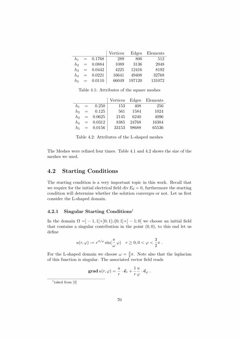
Vertices Edges Elements

h1 = 0.1768 289 800 512h2 = 0.0884 1089 3136 2048h3 = 0.0442 4225 12416 8192h4 = 0.0221 16641 49408 32768h5 = 0.0110 66049 197120 131072

Table 4.1: Attributes of the square meshes

Vertices Edges Elements

h1 = 0.250 153 408 256h2 = 0.125 561 1584 1024h3 = 0.0625 2145 6240 4096h4 = 0.0312 8385 24768 16384h5 = 0.0156 33153 98688 65536

Table 4.2: Attributes of the L-shaped meshes

The Meshes were refined four times. Table 4.1 and 4.2 shows the size of themeshes we used.

4.2 Starting Conditions

The starting condition is a very important topic in this work. Recall thatwe require for the initial electrical field divE0 = 0, furthermore the startingcondition will determine whether the solution converges or not. Let us firstconsider the L-shaped domain.

4.2.1 Singular Starting Conditions1

In the domain Ω =] − 1, 1[×]0; 1[∪[0; 1]×] − 1; 0[ we choose an initial fieldthat contains a singular contribution in the point (0, 0), to this end let usdefine

u(r, ϕ) := rπ/ω sin(π

ωϕ) r ≥ 0, 0 < ϕ <

3

2π .

For the L-shaped domain we choose ω = 32π. Note also that the laplacian

of this function is singular. The associated vector field reads

gradu(r, ϕ) =u

r· ~er +

1

r

u

ϕ· ~eϕ .

1taked from [3]

70

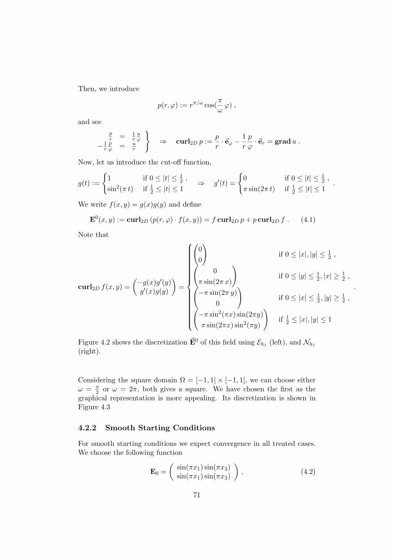
Then, we introduce

p(r, ϕ) := rπ/ω cos(π

ωϕ) ,

and see

pr = 1

ruϕ

−1rpϕ = u

r

⇒ curl2D p :=p

r· ~eϕ −

1

r

p

ϕ· ~er = gradu .

Now, let us introduce the cut-off function,

g(t) :=

1 if 0 ≤ |t| ≤ 12 ,

sin2(π t) if 12 ≤ |t| ≤ 1

⇒ g′(t) =

0 if 0 ≤ |t| ≤ 12 ,

π sin(2π t) if 12 ≤ |t| ≤ 1

.

We write f(x, y) = g(x)g(y) and define

E0(x, y) := curl2D (p(r, ϕ) · f(x, y)) = f curl2D p+ p curl2D f . (4.1)

Note that

curl2D f(x, y) =

(−g(x)g′(y)g′(x)g(y)

)

=

(

0

0

)

if 0 ≤ |x|, |y| ≤ 12 ,

(

0

π sin(2π x)

)

if 0 ≤ |y| ≤ 12 , |x| ≥

12 ,

(

−π sin(2π y)

0

)

if 0 ≤ |x| ≤ 12 , |y| ≥

12 ,

(

−π sin2(πx) sin(2πy)

π sin(2πx) sin2(πy)

)

if 12 ≤ |x|, |y| ≤ 1

.

Figure 4.2 shows the discretization ~E0 of this field using Eh1 (left), and Nh1

(right).

Considering the square domain Ω = [−1, 1] × [−1, 1], we can choose eitherω = π

2 or ω = 2π, both gives a square. We have chosen the first as thegraphical representation is more appealing. Its discretization is shown inFigure 4.3

4.2.2 Smooth Starting Conditions

For smooth starting conditions we expect convergence in all treated cases.We choose the following function

E0 =

(sin(πx1) sin(πx2)sin(πx1) sin(πx2)

)

, (4.2)

71

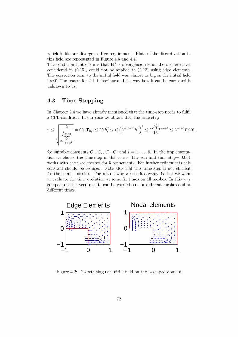
which fulfils our divergence-free requirement. Plots of the discretization tothis field are represented in Figure 4.5 and 4.4.The condition that ensures that ~E0 is divergence-free on the discrete levelconsidered in (2.15), could not be applied to (2.12) using edge elements.The correction term to the initial field was almost as big as the initial fielditself. The reason for this behaviour and the way how it can be corrected isunknown to us.

4.3 Time Stepping

In Chapter 2.4 we have already mentioned that the time-step needs to fulfila CFL-condition. In our case we obtain that the time step

τ ≤

√√√√√√

2

λmax︸︷︷︸

≈C1

|Thi|2

= C2|Thi| ≤ C3h

2i ≤ C

(

2−(i−1)h1

)2≤ C

h2116

2−i+1 ≤ 2−i+10.001 ,

for suitable constants C1, C2, C3, C, and i = 1, . . . , 5. In the implementa-tion we choose the time-step in this sense. The constant time step= 0.001works with the used meshes for 5 refinements. For further refinements thisconstant should be reduced. Note also that this time step is not efficientfor the smaller meshes. The reason why we use it anyway, is that we wantto evaluate the time evolution at some fix times on all meshes. In this waycomparisons between results can be carried out for different meshes and atdifferent times.

−1 0 1−1

0

1Edge Elements

−1 0 1−1

0

1Nodal elements

Figure 4.2: Discrete singular initial field on the L-shaped domain

72

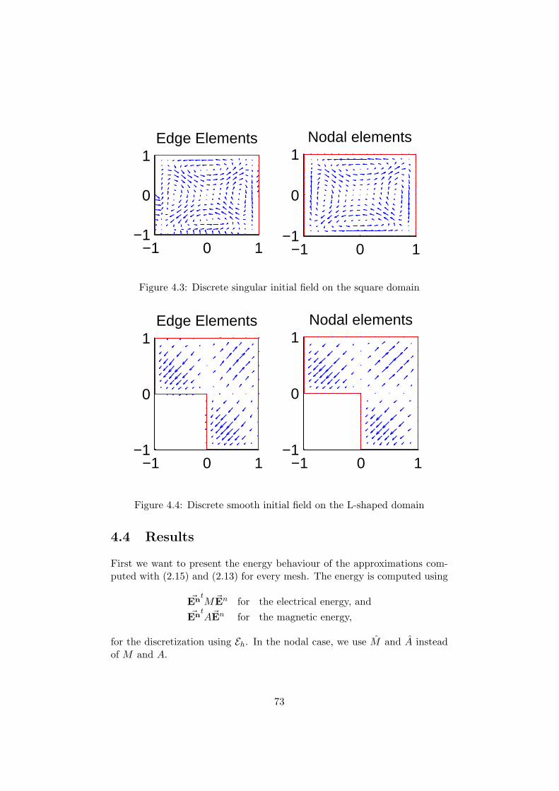
−1 0 1−1

0

1Edge Elements

−1 0 1−1

0

1Nodal elements

Figure 4.3: Discrete singular initial field on the square domain

−1 0 1−1

0

1Edge Elements

−1 0 1−1

0

1Nodal elements

Figure 4.4: Discrete smooth initial field on the L-shaped domain

4.4 Results

First we want to present the energy behaviour of the approximations com-puted with (2.15) and (2.13) for every mesh. The energy is computed using

~EntM~En for the electrical energy, and

~EntA~En for the magnetic energy,

for the discretization using Eh. In the nodal case, we use M and A insteadof M and A.

73

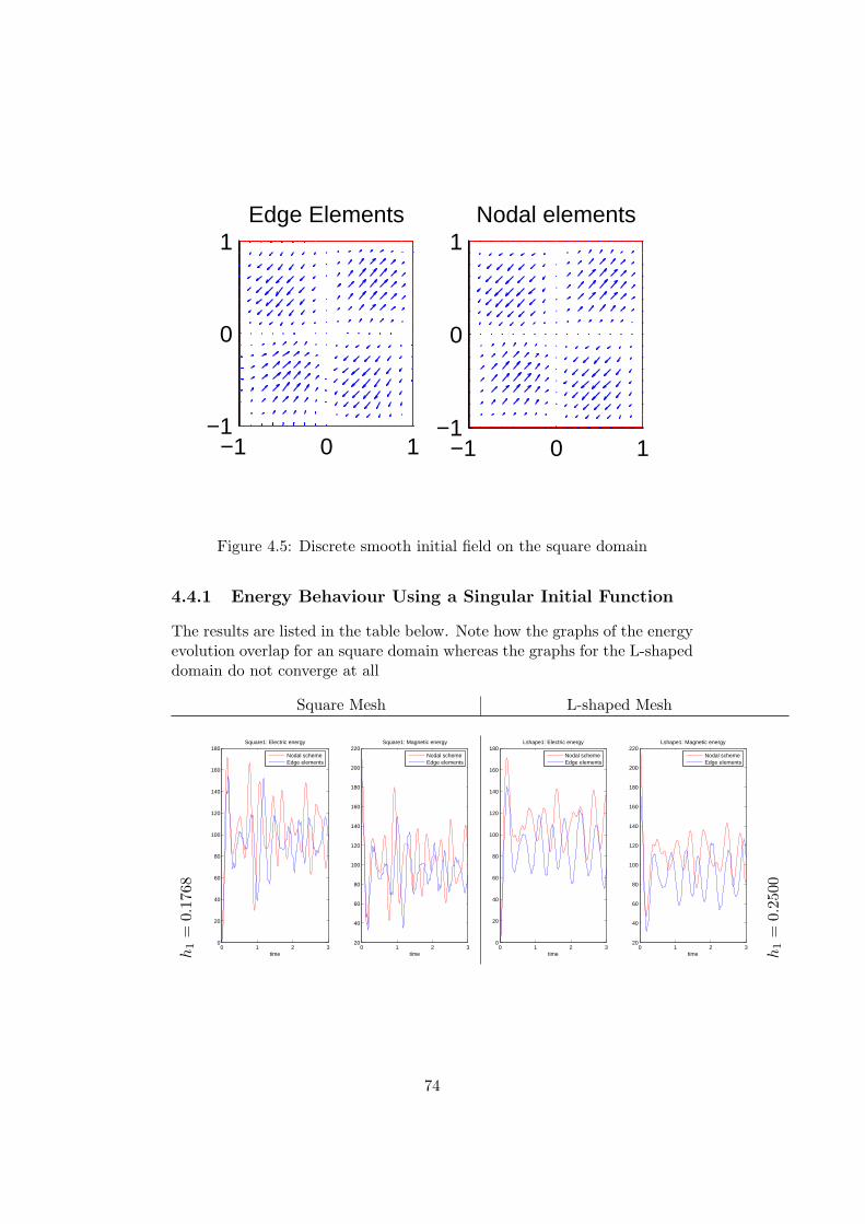
−1 0 1−1

0

1Edge Elements

−1 0 1−1

0

1Nodal elements

Figure 4.5: Discrete smooth initial field on the square domain

4.4.1 Energy Behaviour Using a Singular Initial Function

The results are listed in the table below. Note how the graphs of the energyevolution overlap for an square domain whereas the graphs for the L-shapeddomain do not converge at all

Square Mesh L-shaped Mesh

h1=

0.1768

0 1 2 30

20

40

60

80

100

120

140

160

180

time

Square1: Electric energy

Nodal schemeEdge elements

0 1 2 320

40

60

80

100

120

140

160

180

200

220

time

Square1: Magnetic energy


0 1 2 30

20

40

60

80

100

120

140

160

180

time

Lshape1: Electric energy


0 1 2 320

40

60

80

100

120

140

160

180

200

220

time

Lshape1: Magnetic energy


h1=

0.2500

74

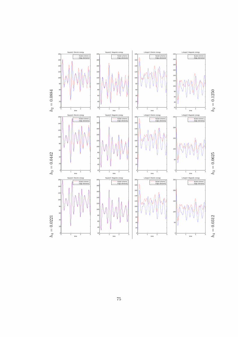
h2=

0.0884

0 1 2 30

20

40

60

80

100

120

140

160

180

time



0 1 2 320

40

60

80

100

120

140

160

180

200

time



0 1 2 30

20

40

60

80

100

120

140

160

180

time



0 1 2 320

40

60

80

100

120

140

160

180

200

220

time



h2=

0.1250

h3=

0.0442

0 1 2 30

20

40

60

80

100

120

140

160

time



0 1 2 320

40

60

80

100

120

140

160

180

200

time



0 1 2 30

20

40

60

80

100

120

140

160

180

time



0 1 2 30

50

100

150

200

250

time



h3=

0.0625

h4=

0.0221

0 1 2 30

20

40

60

80

100

120

140

160

time



0 1 2 320

40

60

80

100

120

140

160

180

200

time



0 1 2 30

20

40

60

80

100

120

140

160

180

200

time



0 1 2 30

50

100

150

200

250

time



h4=

0.0312

75

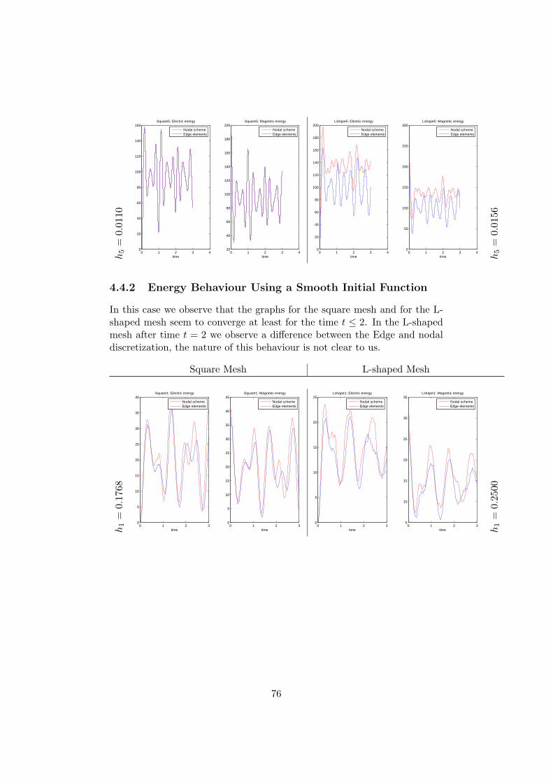
h5=

0.0110

0 1 2 3 40

20

40

60

80

100

120

140

160

time



0 1 2 3 420

40

60

80

100

120

140

160

180

200

time



0 1 2 3 40

20

40

60

80

100

120

140

160

180

200

time



0 1 2 3 40

50

100

150

200

250

300

time



h5=

0.0156

4.4.2 Energy Behaviour Using a Smooth Initial Function

In this case we observe that the graphs for the square mesh and for the L-shaped mesh seem to converge at least for the time t ≤ 2. In the L-shapedmesh after time t = 2 we observe a difference between the Edge and nodaldiscretization, the nature of this behaviour is not clear to us.

Square Mesh L-shaped Mesh

h1=

0.1768

0 1 2 30

5

10

15

20

25

30

35

40

time



0 1 2 30

5

10

15

20

25

30

35

40

45

time



0 1 2 30

5

10

15

20

25

time



0 1 2 35

10

15

20

25

30

35

time



h1=

0.2500

76

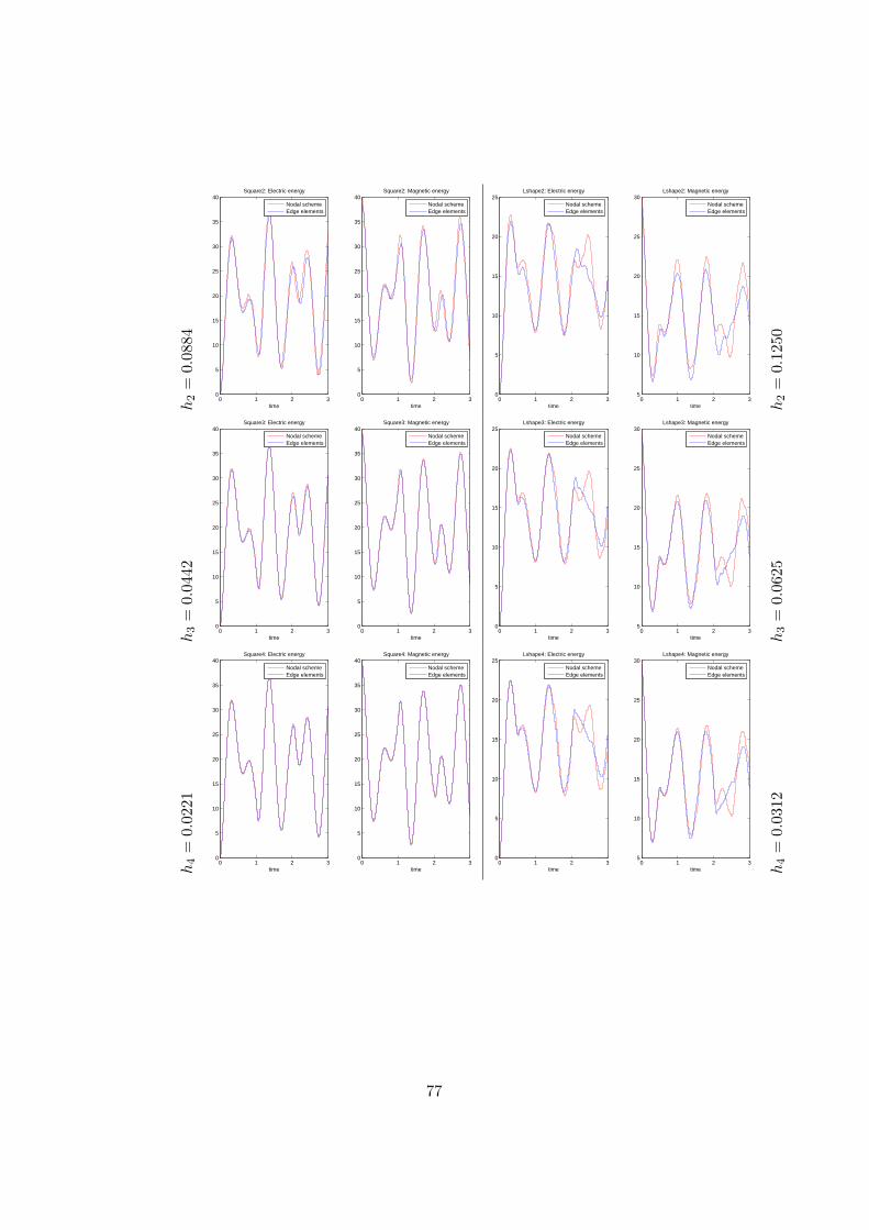
h2=

0.0884

0 1 2 30

5

10

15

20

25

30

35

40

time



0 1 2 30

5

10

15

20

25

30

35

40

time



0 1 2 30

5

10

15

20

25

time



0 1 2 35

10

15

20

25

30

time



h2=

0.1250

h3=

0.0442

0 1 2 30

5

10

15

20

25

30

35

40

time



0 1 2 30

5

10

15

20

25

30

35

40

time



0 1 2 30

5

10

15

20

25

time



0 1 2 35

10

15

20

25

30

time



h3=

0.0625

h4=

0.0221

0 1 2 30

5

10

15

20

25

30

35

40

time



0 1 2 30

5

10

15

20

25

30

35

40

time



0 1 2 30

5

10

15

20

25

time



0 1 2 35

10

15

20

25

30

time



h4=

0.0312

77

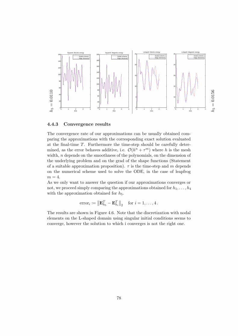
h5=

0.0110

0 1 2 3 40

20

40

60

80

100

120

140

160

time



0 1 2 3 420

40

60

80

100

120

140

160

180

200

time



0 1 2 3 40

5

10

15

20

25

time



0 1 2 3 45

10

15

20

25

30

time



h5=

0.0156

4.4.3 Convergence results

The convergence rate of our approximations can be usually obtained com-paring the approximations with the corresponding exact solution evaluatedat the final-time T . Furthermore the time-step should be carefully deter-mined, as the error behaves additive, i.e. O(hn + τm) where h is the meshwidth, n depends on the smoothness of the polynomials, on the dimension ofthe underlying problem and on the grad of the shape functions (Statementof a suitable approximation proposition). τ is the time-step and m dependson the numerical scheme used to solve the ODE, in the case of leapfrogm = 4.As we only want to answer the question if our approximations converges ornot, we proceed simply comparing the approximations obtained for h1, . . . , h4with the approximation obtained for h5.

errori :=∥∥ET

h5−ET

hi

∥∥2

for i = 1, . . . , 4 .

The results are shown in Figure 4.6. Note that the discretization with nodalelements on the L-shaped domain using singular initial conditions seems toconverge, however the solution to which i converges is not the right one.

78

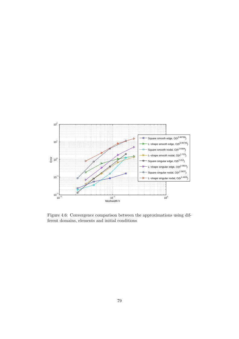
10−2

10−1

100

10−2

10−1

100

101

102

Meshwidth h

Err

or

Square smooth edge, O(h0.90786)

L−shape smooth edge, O(h0.99745)

Square smooth nodal, O(h2.0304)

L−shape smooth nodal, O(h1.723)

Square singular edge, O(h2.412)

L−shape singular edge, O(h2.0914)

Square singular nodal, O(h2.3637)

L−shape singular nodal, O(h1.4426)

Figure 4.6: Convergence comparison between the approximations using dif-ferent domains, elements and initial conditions

79

Bibliography

[1] R. Hiptmair. Finite Elements in computational electromagnetism, Uni-versitat Tubingen, Acta Numerica (2002), pp.237-339

[2] D. Sun, J. Manges, X. Yuan, Z. Cendes. Spurious Modes in Finite-Element Methods, IEEE Antennas and Propagation Magazine, Vol. 37,No. 5, October 1995.

[3] D. Arnold, R. Hiptmair. Discretizing transient Maxwell’s equations,

80

spurious solutions for transient maxwell equations … zurich¨ spurious solutions for transient...

Documents