Michigan Technological UniversityDigital Commons @ Michigan

Tech

Dissertations, Master's Theses and Master's Reports

2016

SPRING DISCHARGE MODELING: A CASESTUDY IN THE COMARCA NGÄBE-BUGLÉ,WESTERN PANAMAJordan MayerMichigan Technological University, jamayer@mtu.edu

Copyright 2016 Jordan Mayer

Follow this and additional works at: http://digitalcommons.mtu.edu/etdr

Recommended CitationMayer, Jordan, "SPRING DISCHARGE MODELING: A CASE STUDY IN THE COMARCA NGÄBE-BUGLÉ, WESTERNPANAMA", Open Access Master's Report, Michigan Technological University, 2016.http://digitalcommons.mtu.edu/etdr/191

SPRING DISCHARGE MODELING: A CASE STUDY IN THE COMARCA NGÄBE-BUGLÉ, WESTERN PANAMA

By

Jordan A. Mayer

A REPORT

Submitted in partial fulfillment of the requirements for the degree of

MASTER OF SCIENCE

In Geology

MICHIGAN TECHNOLOGICAL UNIVERSITY

2016

© 2016 Jordan A. Mayer

This report has been approved in partial fulfillment of the requirements for the Degree of MASTER OF SCIENCE in Geology.

Department of Geological & Mining Engineering and Sciences

Report Advisor: Dr. John Gierke

Committee Member: Dr. Alex Mayer

Committee Member: Dr. David Watkins

Department Chair: Dr. John Gierke

3

Table of Contents Acknowledgements ......................................................................................................................... 4

Abstract ........................................................................................................................................... 5

1.0 Introduction ............................................................................................................................... 6

1.1 Cultural Context .................................................................................................................................. 6

1.2 Motivation ........................................................................................................................................... 7

1.3 Scope of Study/Objectives .................................................................................................................. 7

2.0 Background ............................................................................................................................... 8

2.1 Geography ........................................................................................................................................... 8

2.2 Hydrogeology ................................................................................................................................... 11

3.0 Methods................................................................................................................................... 12

3.1 Water Budget .................................................................................................................................... 12

3.1.1 Weather Data Collection ............................................................................................................ 13

3.1.2 Evapotranspiration ..................................................................................................................... 14

3.1.3 NRCS Curve Number Method ................................................................................................... 14

3.1.4 Hydraulic Conductivity .............................................................................................................. 16

3.2 Spring Base Flow Recession ............................................................................................................. 18

3.3 Groundwater Flow Model ................................................................................................................. 19

3.3.1 Hewett-Hibbert Test Model ....................................................................................................... 20

3.3.2 Salto Dupi Flow Model Configuration ...................................................................................... 21

3.3.3 Salto Dupi Flow Model Configuration and Calibration ............................................................. 22

3.3.3 Climate Scenario Testing ........................................................................................................... 23

4.0 Results and Discussion ........................................................................................................... 24

4.1 Water Budget .................................................................................................................................... 24

4.2 Hydraulic Conductivity ..................................................................................................................... 27

4.3 Hewlett-Hibbert Model ..................................................................................................................... 27

4.4 Salto Dupi Model .............................................................................................................................. 30

4.5 Climate Scenario Testing .................................................................................................................. 34

4.6 Impact on the Ngäbe People ............................................................................................................. 35

5.0 Conclusion .............................................................................................................................. 36

Works Cited .................................................................................................................................. 37

4

Acknowledgements I would like to thank Peace Corps and Michigan Technological University for the

opportunity to live and serve in another country for two years and do what I am passionate about.

I would like to thank Dr. John Gierke for all his support both in the field and on campus. I would

like to thank Dr. Alex Mayer and Dr. David Watkins for serving on my committee.

I would like to thank my friends and family for all your support through Peace Corps and

beyond. With your support I was able to make the most out of my PC experience. A thank you to

my Peace Corps Volunteer neighbors who helped me with data collection, offered a place to

stay, and kept me company.

Por ultimo, me gustaría agradecer a la gente de Salto Dupi. Gracias por hacerme uno de

suyos. Un agradecimiento especial a Alvaro Benjerano por ser mi mentor y amigo.

5

Abstract Contact (seepage) springs are frequently the only source of potable drinking water for the

Ngäbe people located in the Comarca Ngäbe-Buglé, Western Panama. Dry season flows

drastically diminish and sometimes dry up, greatly affecting locals’ access to clean drinking

water. This study uses MODFLOW 2005 to model two aquifer systems. One is a lab-created,

idealized system, and the other is a small, steeply-sloping aquifer in the Comarca Ngäbe-Buglé.

Modeling the idealized aquifer demonstrated that MODFLOW 2005 has the capacity to model

the dewatering of a steeply sloping aquifer. Modeling the field based aquifer demonstrated that a

changing climate (increased temperature and decreased rainfall) will affect wet season discharge

and have a small effect on late dry season discharge.

6

1.0 Introduction Panama is a country located in the southern portion of Central America between

Columbia and Costa Rica. It is home to the Comarca Ngäbe-Buglé which is located in the

western portion of the country. This study looks at the drainage of two separate aquifer systems.

One an idealized sloping aquifer in the lab created by Hewlett and Hibbert (Hewlett, 1963), and

the other a sloping aquifer in western Panama. MODFLOW 2005 was used to model both of the

aquifer’s discharges and compare it to the observed data. Different recharge rates were entered

into the Panama model to forecast how a changing climate will affect dry season flows in the

Comarca Ngäbe-Buglé.

1.1 Cultural Context As a Peace Corps Volunteer (PCV) serving as a sustainable agricultural systems, I

volunteered in Panama from June 19, 2013 to August 21, 2015. I was assigned to Salto Dupi, a

medium sized village in the Comarca Ngäbe-Buglé, roughly 350 km west of Panama City. Salto

Dupi is a rural village with limited access to electricity, running water, and modern

transportation. The region is defined by steep, mountainous terrain and a tropical climate.

My work as a PCV included teaching soil conservation techniques to rural farmers. Much

time was spent teaching locals how to prune coffee and cacao in order to increase their yields

and better their standard of living. In addition to agricultural work, I spent time educating locals

about the springs in the area. Locals had many questions about where spring water is derived,

how they could prevent spring flows from diminishing in the dry season, and how they could use

spring water for crop irrigation to extend the growing season into the dry season. This proved to

be a natural connection between Peace Corps work and my geology background.

The Comarca Ngäbe-Buglé is primarily composed of the Ngäbe people. The Ngäbe

people, also known as the Guaymi, represent the largest population of indigenous people in

Panama at 65.5%. They traditionally live in small family compounds with no access to running

water, electricity, and sanitation facilities. Because of this, 73% of households live in extreme

poverty (Inchauste & Cancho, 2010). As of 2008, 71% of Ngäbes were receiving their water

from local mountainous springs or aqueducts, which ultimately are fed by mountainous springs

(Inchauste & Cancho, 2010).These springs in many cases are the only source of potable drinking

water in the area, thus the Ngäbe people are highly dependent on these springs for daily life.

7

1.2 Motivation Growing population worldwide continues to put stress on water resources. Not only is

there an increased demand for potable water, but more water is needed for agriculture to provide

increased yields for a growing population. These factors will put more pressure on an already

threatened resource (Molden, 2007). These problems will only be exacerbated with global

climate change. Rainfall in Panama is forecasted to change up to 50% by 2100, and temperatures

are expected to increase by 3°C to 6°C due to a changing climate (Magrin & Marengo, 2014).

Higher temperatures coupled with an alteration of the wet/dry season cycle could have extreme

effects on the Ngäbe people.

Panama’s climate has distinct wet and dry seasons. Groundwater recharge and storage in

the wet season provides base flow throughout the dry season which is the sole source of potable

drinking water. Being able to better predict how climate change may affect these springs could

provide more resiliency to locals and allow them to better prepare for a changing climate. As a

PCV living in the community, there was great potential to study these mountainous springs and

then pass this knowledge on to the local Ngäbe people.

As a resident of the community, I was proximal to many springs. This presented an

opportunity to collect flow data on these springs to monitor them temporally. It also presented

the opportunity to collect site specific climatic data with a high temporal resolution.

1.3 Scope of Study/Objectives This study focused on a small (<1 hectare), shallow, steeply sloping aquifer in the

Comarca Ngäbe-Buglé in western Panama. Eleven months of meteorological data were collected

from August 2014-July 2015 for this study. Flow measurements were recorded for those 11

months on a spring draining this aquifer. Soil infiltration rates were deduced using permeameter

data collected on the watershed. Groundwater Modeling Systems (AquaveoTM, Provo, Utah) was

used to investigate how sensitive spring discharge of the aquifer is to different aquifer parameters

and a changing climate.

The overall goal of this study was to forecast how a changing climate will affect late dry season

flows. To achieve this goal, the following objectives were created:

8

• Perform a water budget analysis on the spring catchment.

• Model published observations from an idealized, steeply sloping aquifer apparatus using

a groundwater flow model (MODFLOW-2005) to ascertain how to use MODFLOW-

2005 to simulate the spring catchment.

• Ascertain aquifer properties that affect summer base flow conditions using MODFLOW

2005.

• Compare different model geometries in MODFLOW 2005 and compare them to base

flow conditions observed in the field.

• Once an appropriate model geometry is selected, calibrate MODFLOW 2005 to observed

data in the field.

• Use the calibrated MODFLOW 2005 model to evaluate how various climatic scenarios

will affect summer base flow conditions.

2.0 Background

2.1 Geography

Panama is an equatorial (N 7-10˚) country in Central America. It is bordered by the

Atlantic Ocean to the north and the Pacific Ocean to the south, as well as Costa Rica to the west

and Columbia to the east. A defining feature of the country is the Cordillera Central, a spine of

mountains that trends east-west and forms the continental divide.

Panama experiences a tropical climate. Temperatures remain fairly constant around 25°C

at night and 30°C during the daytime throughout the year. The western highlands stay relatively

wet and cool throughout most of the year due to their higher elevation. There are distinct wet and

dry seasons, with the dry season starting around the end of December and the wet season starting

in late April or early May. Much of the country receives annually between 3-4 meters of rainfall

(ESTESA, 2016).

The study site was based in Salto Dupi, a small indigenous community located roughly

350 km west of Panama City in the Comarca Ngäbe-Buglé (Figure 1). The community is located

9

at 8.350137N, 81.888083W, which is in the foothills of the central spine of the mountains on the

Pacific side of the country. The author lived in Salto Dupi for two years as a PCV and was

proximal to the study site (Figure 2). The area of study is defined by steep mountainous terrain.

Small streams are abundant and have cut steep valleys down to bedrock. This contact with

bedrock in the valleys is usually the location of contact springs.

Figure 1: Map of Panama showing study site. (Map created in ArcGIS 10.3.1, Basemap and outline of the Comarca obtained from ArcGIS online. Projection: WGS 1984.)

10

Figure 2: Satellite image of the author’s community (Map created using Google Maps map creator. Imagery Date: 3/5/2006)

Land use is dedicated mostly to agriculture, including the cultivation of rice, banana,

corn, beans, coffee, and cacao. The land cover of the watershed studied was a mix of coffee and

cacao fields. Banana and large wood (timber) trees were also present but at much lower density.

Cacao and coffee trees were established, from 5 to 20 years old. They were spaced roughly 1.5

meters apart. Banana and large wood trees were spaced at 10 meters apart. The ground surface

was shaded most of the time due to the full canopy cover. Soil was covered by a small amount of

grass and small plants. This left soil mostly bare. Little decomposing organic matter was present

on the soil surface. Slash and burn agriculture is still practiced by most of the community

members. This process leaves the loose unconsolidated soil exposed to rainfall. The exposed

soils combined with high rain intensity promotes high rates of erosion and has left the soil in

very poor condition.

11

2.2 Hydrogeology The geology in Salto Dupi is dominated by highly weathered ocean sediments that were

deposited during the Miocene and Pliocene. Underlining these ocean sediments are Tertiary and

Quaternary volcanics (Coates & Obando, 1996).

High rates of erosion have cut steep valleys into the ocean sediments. At the base of these

valleys, erosion has cut down to bedrock. Valleys typically have ephemeral or perennial streams

that are fed by springs. These springs are located where surface topography contacts bedrock to

form seepage/contact springs (Figure 3). In addition to spring flow, streams in the area are fed

by surface runoff during most rain events. Because of the steep topographic gradient, surface

runoff flows downslope relatively quickly. During the dry season, flow from springs is the only

source of streamflow. In the dry season, flow decreases in springs and thus, some streams dry up.

Figure 3: Conceptual model of seepage springs (Drawn by author)

Springs are very important for the local Ngäbe people, often providing the only source of

clean drinking water. Some community members have built crude spring boxes around springs to

reduce sediment load from surface runoff. Spring boxes also serve as crude catchment systems to

funnel spring flow into PVC pipes which channel water downslope into crude water distribution

systems. More information on the importance of spring catchments on rural health can be found

in (Fry, 2004). More information about spring catchments in the Comarca Ngäbe-Buglé can be

found in (Jones, 2014).

12

3.0 Methods To better understand steeply sloping aquifers in the tropics and simulate how a changing

climate might affect base flow discharge, a numerical model was developed and applied to

simulate the observed flows in the spring catchment. This aquifer was selected because of its

size, uniformity of land cover, and proximity to the author’s work area. Spring flow discharge

was continuously captured by the owner of the watershed before the author’s arrival, allowing

for easy spring base flow measurements. The spring catchment area was delineated using the

track feature on a Garmin GPS (GPSmap 60CSx, Olathe, KS). GPS points were taken every 30

seconds while the author walked the border of the watershed. The border of the aquifer was

defined by a ridgeline to the west and north, and steeply sloping valley to the east.

Hydrologic and meteorological data was collected for this aquifer along with spring flow

measurements and soil infiltration rates. Spring flow data was collected for 11 months using a

DLJ totalizer meter (DLJ50, Hackensack, NJ). Hydraulic conductivity was measured on the

aquifer using a soil infiltrometer and the Glover solution (Amoozegar, 1989). Evapotranspiration

was estimated using climatic data collected by the author in site. The NRCS curve number

method was used to estimate surface storm related runoff (USDA, 1986). Hydrological data was

entered into Groundwater Modeling Software 10.0 (GMS) by Aquaveo, and MODFLOW 2005

was used to model spring discharge. Computed flow was compared to observed flow, and aquifer

geometry was calibrated to match flows. Once calibrated, different climate scenarios were

entered into the groundwater model, and spring discharge was forecasted.

3.1 Water Budget The water budget, or water balance, is a useful tool for understanding and evaluating

components of the hydrologic cycle. A water balance assumes a conservation of water (mass or,

as is often the case, because water density can be treated as a constant, volume) for a closed

system such as a watershed or aquifer. In this study, it was assumed that all recharge served as

aquifer storage or aquifer discharge.

Recharge was broken down into three components in this study and is reflected by the

following equation:

𝑅𝑅 = 𝑃𝑃 − 𝐸𝐸𝐸𝐸 − 𝑄𝑄𝑟𝑟𝑟𝑟

13

Where:

R = Recharge

P = Precipitation

ET = Evapotranspiration

Qro = Surface runoff

A year was chosen as the time scale for this study because of available data. In this study,

water balance parameters were entered into groundwater modeling software to deduce how

hydraulic conductivity and aquifer storage properties affect flow over time.

3.1.1 Weather Data Collection

The project site has a climate that is defined as hot and humid. There is a network of

weather stations in Panama operated by the Panamanian electric transmission network (ESTESA,

2016). The network had two stations within 5 miles of the project site. In addition to these

stations, an Ambient Weather WS 1090 wireless home weather station was installed in the

author’s home to record weather in situ. This weather station has a data logging feature with a

30-minute temporal resolution. Data was collected starting Aug 25, 2014 until July 24, 2015.

Temperature, relative humidity, rainfall, wind speed and wind direction were collected every

thirty minutes. Temperature and rainfall accuracy were verified with a hand thermometer and

volumetric cylinder, respectively.

A total of 3.58 meters of rainfall was measured for the 11-month period that the weather

station was installed. Missing data spanned from mid-July to mid-August because the author had

to leave the study site in mid-July. Measured rainfall was compared to ETESA data for the

stations proximal to the study site. An amount of 0.3 meters of rainfall (0.1 meter in July and 0.2

meters in August) was added in order to compensate for the lack of a month of data. 0.3 meters

was chosen to achieve a year total of 3.88 meters. This is 0.2 meters less than the average

proximal to the study site. 0.3 was chosen because the study year was a dry year and climate is

becoming dryer in the study site.

In the study site, seasons are defined by differences in precipitation rather than a

difference in temperature. The dry season typically starts at the end of December, and the wet

usually begins at the start of May. During the dry season there were 3 rain events that resulted in

a total of 7.5 mm of rainfall. These small and very localized storms served only to wet the

14

ground cover and evaporated within minutes. Thus they were not included in the total rainfall.

The last rainfall of the wet season in 2014 occurred on Dec 20, 2014, and the first rainfall

initiating the 2015 wet season started on April 20, 2015. The first appreciable amount of rain in

the 2015 wet season happened on April 29, 2015 (82 mm). These dates were used to define the

end and the start of the wet season in the MODFLOW model.

3.1.2 Evapotranspiration

Evapotranspiration (ET) can be a very large portion of any water balance, but it is often

one of the hardest parameters to measure. Various methods have been developed for measuring

ET, but they are often extensive and expensive. Many methods have been developed for

estimating potential evapotranspiration (PET), most notably the Thornthwaite-Mather

(Thornthwaite, 1948) and the Penman-Monteith (Penman, 1948). Both of these methods use

average temperatures and relative humidity to estimate PET. For this study, both of these

methods were considered for analysis. The Penman-Monteith method was performed using daily

maximum and minimum temperature and relative humidity that was collected in the study site

(Richard, Luis, & Smith, 1998). This method also took into account solar shine hours that were

collected by a government-operated weather station about 31 km away. The Thornthwaite-

Mather method was performed using monthly average temperature collected in the study site.

PET was calculated using the Hamon equation (Dingman, 2015). Actual ET was estimated using

a soil moisture budget. Assumed soil field capacity of 30% and a rooting depth of 0.5 meters

were used. The results were not sensitive to these assumed values.

3.1.3 NRCS Curve Number Method

The amount of rainfall that actually infiltrates into the aquifer is dependent on the slope

of the surface, land cover, rainfall intensity and duration, and the nature of the soil. In the

mountainous tropics, high precipitation intensity and steep topography causes high amounts of

surface runoff. Thus, it is important to estimate this runoff so it can be accurately accounted for

in the water balance. The United States Department of Agriculture’s Natural Resources

Conservation Service (NRCS) developed the curve number method from runoff observed from

15

test plots (USDA, 1986). It is used in the federal, state, and private sectors to estimate the

amount of surface runoff that is present for a given precipitation event.

The NRCS curve method assigns a curve number from 30 to 100, with higher numbers

resulting in high runoff potential. A forest cover type was chosen for the study site due to the

large amount of woody plants in the area. Poor hydrological conditions and a poor soil type

yielded a curve number of 83 within this cover type. This curve number was used to calculate

surface runoff.

Another important aspect to consider when simulating soil infiltration is the antecedent

moisture condition (AMC). This relates to the soil moisture conditions prior to the rain event.

Dry soil will absorb more moisture from a storm event than wet soil. The average moisture curve

number (AMC II) must be adjusted for dry (AMC I) or wet (AMC III) soils. The following

equations were used to convert AMC II to an antecedent wet and dry curve numbers (USDA,

1986).

AMC I = AMC II / (2.3) – (0.013*AMCII)

AMC III = AMC II / (0.43) – (0.0057*AMCII)

Where:

AMC I = Antecedent dry conditions curve number

AMC II = Average conditions curve number

AMC III = Antecedent wet conditions curve number

Based on the equations above, for example, if in the previous 5 days it rained more than

53 mm, the soil had wet antecedent conditions and a curve number of 93.5 was used. If in the

previous 5 days it rained 35-53 mm, the soil had average antecedent conditions and a curve

number of 83 was used. If in the previous 5 days it rained less than 35 mm, the soil had

antecedent dry conditions and a curve number of 72.7 was used. The NRCS method was

performed for each storm event. A storm event was defined as any amount of rain that fell in a

given day.

16

3.1.4 Hydraulic Conductivity

Saturated hydraulic conductivity was measured in the vadose zone using an

amoozemeter. The infiltrometer methodology was developed by A. Amoozegar and it allows one

to determine the saturated hydraulic conductivity (Ksat) of the vadose zone with limited materials

(Amoozegar, 1989). This method was advantageous because it allows Ksat to be determined in

about an hour using small boreholes and a few liters of water. Figure 4 shows the general design

of the amoozemeter used. A borehole with a diameter of 6.2 cm and 56.6 cm deep was dug using

a PVC auger fabricated by the author. The permeameter was filled with water and then inverted

into the borehole. Water flowed out of the permeameter forming a constant head in the borehole.

The flow (change in height in the reservoir over time) was recorded until the flow reached a

steady state.

17

Figure 4: Design of the amoozemeter used in this study (drawn by Author)

The Glover solution (Zangar, 1953) was used to determine Ksat from a flow rate

determined from the amoozemeter. The Glover solution only takes into consideration the

saturated flow emanating from the borehole. The equation has been used to provide an accurate

estimation of Ksat. The equation is as follows:

𝑲𝑲𝒔𝒔𝒔𝒔𝒔𝒔 = 𝑸𝑸

⎝

⎜⎛𝐬𝐬𝐬𝐬𝐬𝐬𝐬𝐬−𝟏𝟏 𝑯𝑯𝒓𝒓 −���

𝒓𝒓𝑯𝑯�

𝟐𝟐+ 𝟏𝟏� + �𝒓𝒓𝑯𝑯�

𝟐𝟐𝟐𝟐𝟐𝟐

⎠

⎟⎞

18

Where:

Ksat = Saturated hydraulic conductivity (cm/day)

Q = Steady flow rate from amoozemeter (cc/day)

H = Height of water in borehole (cm)

r = radius of borehole (cm)

A total of three Ksat tests were conducted in the area. An average Ksat of 10 cm/day was

measured for the area. A Ksat of 16 cm/day was measured in the aquifer that was studied. This

value was chosen as the saturated hydraulic conductivity of the study site to be entered into the

groundwater flow model because it was collected in the watershed under study.

3.2 Spring Base Flow Recession Key aquifer parameters can be deduced from performing a base flow recession analysis.

In this study, a base flow recession analysis was performed during the dry season to deduce

aquifer storage and aquifer geometry. Spring discharge rates were collected using a DLJ totalizer

meter. Spring discharge was collected and funneled into a 2-inch pvc pipe by a crude spring box

that was built prior to the author’s arrival (Figure 5).

19

Figure 5: Picture of the spring box and seepage spring for this study (Photo taken by author)

The base of the spring box was bedrock and assumed to be impermeable. It was assumed

that the spring box only captured spring flow and not surface runoff during storm events because

the spring box was covered during normal operation. The author visited the DLJ meter

throughout the 11 months to record the time and total gallons of discharge. This discharge

provided a hydrograph to which a flow model could be calibrated.

3.3 Groundwater Flow Model A three-dimensional groundwater flow model was constructed in Groundwater Modeling

Systems 10.0.1 (GMS). GMS is computer software that combines a GIS user interface with

United States Geological Survey’s (USGS) MODFLOW package (Aquaveo, 2016). GMS was

used for this study because of its ability to incorporate geographic data such as location and

elevations and its ability to map them to the MODFLOW flow equations. MODFLOW is a

modular finite-difference flow model that was developed by USGS (McDonald & Harbaugh,

1988). This study used the 2005 version of MODFLOW. MODFLOW incorporates aquifer

parameters such as hydraulic conductivity, specific storage, sources, and sinks and applies them

to 3D flow calculations.

20

3.3.1 Hewett-Hibbert Test Model

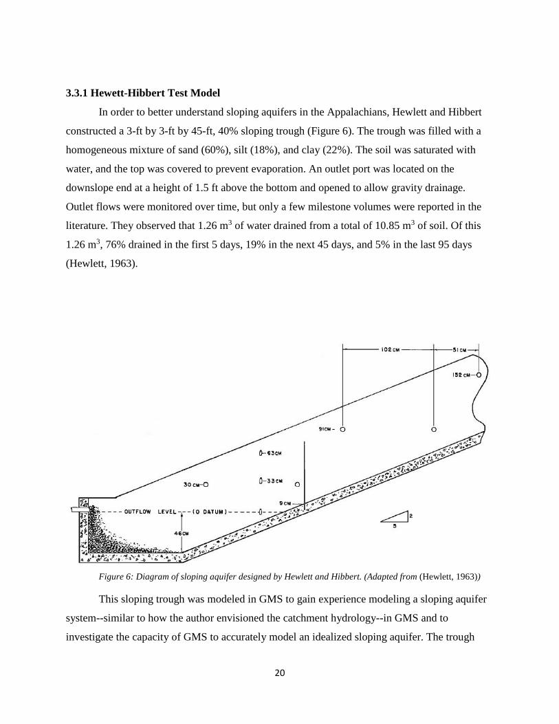
In order to better understand sloping aquifers in the Appalachians, Hewlett and Hibbert

constructed a 3-ft by 3-ft by 45-ft, 40% sloping trough (Figure 6). The trough was filled with a

homogeneous mixture of sand (60%), silt (18%), and clay (22%). The soil was saturated with

water, and the top was covered to prevent evaporation. An outlet port was located on the

downslope end at a height of 1.5 ft above the bottom and opened to allow gravity drainage.

Outlet flows were monitored over time, but only a few milestone volumes were reported in the

literature. They observed that 1.26 m3 of water drained from a total of 10.85 m3 of soil. Of this

1.26 m3, 76% drained in the first 5 days, 19% in the next 45 days, and 5% in the last 95 days

(Hewlett, 1963).

Figure 6: Diagram of sloping aquifer designed by Hewlett and Hibbert. (Adapted from (Hewlett, 1963))

This sloping trough was modeled in GMS to gain experience modeling a sloping aquifer

system--similar to how the author envisioned the catchment hydrology--in GMS and to

investigate the capacity of GMS to accurately model an idealized sloping aquifer. The trough

21

was represented by a uniform grid that was 3 cells wide, 1 cell high, and 45 cells long, each

having a cubic volume of 3 ft3. A MODFLOW 2005 model was initiated for the grid. The model

was set to transient, and a stress period of 145 days was used. A drain was placed at the lower

end of the model at an elevation of 1.5 feet. A drain was used because it allows water to flow out

of the model as long as the surrounding head is above the elevation of the drain. If head falls

below the elevation of the drain, the flow becomes zero. Drain conductance was set at 500

ft2/day, and this conductance was high enough that all resistance to flow was due to the hydraulic

conductivity of the soil in the trough. Starting heads were set to the surface elevation.

It is known that 1.26 m3 (44.5 cubic feet) was drained from this trough over 145 days.

This provided a target total discharge for the model. Specific storage was set at 0.0001

(dimensionless) and had little effect on the model due to this being modeled as an unconfined

aquifer. An initial specific yield of 2% and a hydraulic conductivity of 3 ft/day were used. The

model was allowed to drain, and flow variations with time were observed. Specific yield was

adjusted to 0.113 to achieve a total volume out of 44.5 cubic feet. Hydraulic conductivity was

adjusted to 2.45 ft/day to achieve 76% volume outflow in the first 5 days and the remaining 24%

in the following 140 days of the simulation. The hydraulic conductivity of the soil was not

independently measured. The model results are presented in Section 4.3.

3.3.2 Salto Dupi Flow Model Configuration

A model was created in GMS for the author’s watershed in Salto Dupi using a similar

approach to that used for the Hewlett-Hibbert model. Surface topography and lateral boundaries

were more irregular and complex in the field, so these had to be incorporated into the model in a

different fashion than the simple specifications used for the Hewlett-Hibbert experiment. GPS

coordinates from the watershed delineation were imported into GMS. These coordinates served

as the boundary of the watershed and also served as the surface elevations in the model. A

MODFLOW 2005 simulation was created and the GIS data was applied to it to form the model

boundaries. The model was set to transient conditions, and four stress periods were set up to

represent evapotranspiration estimates for January, February, March, and April.

Evapotranspiration rates were estimated to decrease during the dry season because the water

table would naturally deepen with drainage. The rates were estimated using the Thornthwaite

type water budget method. These months coincide with the dry season in the study site. Cell size

22

was 1.5 by 1.5 meters in the horizontal, and 12 meters vertically, with a total of 2765 cells and

total area of 6221.25 m2. The starting geometry of the aquifer was a uniform sloping lens that

mimicked surface topography. This lens was set to become flat and pinch out at the drain

elevation. The drain was set at 359.5 mamls and was four cells wide. The drain conductance was

set to 500 m2/day for each of the four drain cells. Like in the Hewlett-Hibbert simulations, this

conductance was nonrestrictive. Starting heads were set to the surface elevation because the

bottom elevations of the aquifer were unknown and it was conceptualized that the water table

mimicked the bottom topography at the beginning of the dry season.

3.3.3 Salto Dupi Flow Model Configuration and Calibration

Modeling the Hewlett-Hibbert trough in GMS demonstrated that modeling the

dewatering of a sloping aquifer can allow one to use known aquifer parameters to estimate

unknown parameters. Spring discharge, hydraulic conductivity, and groundwater recharge were

estimated from measurements and used to calibrate aquifer thickness for the aquifer in Dupi.

Specific storage was set at 0.0001 (dimensionless). Hydraulic conductivity was set at 0.16

m/day. Evapotranspiration was modeled as a negative recharge to accurately depict the water

leaving the surface of the aquifer. This was entered at -0.0026 m/day, -0.0013 m/day, -0.0005

m/day, and 0 m/day for January, February, March, and April, respectively. Although specific

yield was an unknown, it was entered as 2%, which is consistent with average values for clays

from textbooks (Fetter, 2001). Aquifer thickness was manually adjusted until modeled discharge

matched observed flows.

A thickness of 10 meters was used for the first simulation of the model. Spring discharge

values were taken from the model and entered into a spreadsheet to visualize and calculate spring

discharge. A total volume of water discharged from the spring was calculated. The aquifer

thickness was changed until the modeled total discharge during the dry season matched the

observed total of 435 cubic meters, resulting in a model-adjusted aquifer thickness of 12 m.

After calibrating thickness, additional stress periods were added to the model to simulate

the wet season. Table 1 shows the parameters that were used for the wet season model and an

explanation of the values. Spring discharge was plotted in the spreadsheet.

23

Table 1: Parameters and stress periods that were entered into the groundwater flow model

3.3.3 Climate Scenario Testing

In order to estimate the sensitivity of the model to a changing climate and to forecast the

effect that a changing climate has on the dry season spring flows, different climate scenarios

were implemented into the model. The 2014 Intergovernmental Panel on Climate Change

predicts that average temperatures could increase by 3˚C by 2050 in Panama (Magrin &

Aquifer Parameters Values Used Explanation Cell Area 1.5 by 1.5 meters

Aquifer thickness

12 meters

Thickness was calibrated using

observed flow data from the spring

Specific storage 0.0001 Estimated (not significant because this is a unconfined aquifer)

Specific yield 0.02 Estimated using published data

Hydraulic conductivity 0.16 m/day Measured in the study site with an

amoozemeter Stress Periods Recharge Rate (M/Day)

5/1/2014 0.0045 Calculated using water budget and collected

data 12/20/2014 -0.0026 Calculated using TM 2/1/2015 -0.0013 Calculated using TM 3/1/2015 -0.0005 Calculated using TM 4/1/2015 0 No recharge 5/1/2015 0.05 Initial recharge rate to

initiate recharge 5/2/2015 0.0045 Calculated using water

budget and collected data

12/20/2015 end

24

Marengo, 2014). This 3˚C increase was entered into the Thornthwaite ET equation to estimate

changes to ET. It was entered as a 3 ˚C increase for each month’s average temperature. The

resulting change in PET was then used to estimate actual ET which was incorporated into a new

water budget. The new recharge rate was then entered into the model and changes in spring

flows were calculated.

Climate models for Panama predict a change in yearly precipitation by up the 50% by

2100 (Magrin & Marengo, 2014). A 10% change in precipitation total was modeled to observe

the effect it had on dry season spring discharge. Every rain event was multiplied by 0.9 to

simulate a decrease of precipitation of 10%. The NRCS method was performed to estimate the

runoff. ET was subtracted and a recharge rate for the model was obtained. This was entered into

the model and flow was observed. Table 2 shows the parameters that were entered into the model

for both the 3 degree increase in temperature and the 10% decrease in precipitation.

Climate Scenario Inputs

Recharge Rate (m/day) Stress Period 3˚C Increase 10%

decrease 5/1/2014 0.0037 0.0042

12/20/2014 -0.03 -0.0027 2/1/2015 -0.0012 -0.0013 3/1/2015 -0.0004 -0.0005 4/1/2015 0 0 5/1/2015 0.05 0.05 5/2/2015 0.0037 0.0042

12/20/2015 end end Table 2: Stress periods and values used in the model for different climate scenarios

4.0 Results and Discussion 4.1 Water Budget Precipitation:

The total precipitation for the year in the study site was 3880 mm, all falling within the

wet season from April 20 to December 20. The rainiest month was September with 831mm of

total rainfall. Table 3 summarizes rainfall on a monthly basis in the study site. Amounts of 100

mm and 200 mm were added to July and August, respectively, to make up for a month of

missing data. These were selected based on historical data that was collected by a government

station roughly 7 kilometers from the study site (ESTESA, 2016). The dry season is January-

25

April. April was modeled in the dry season because 169 mm of precipitation fell in the last 9

days of the month, with the majority of that on the last two days.

Measured Precipitation Month Rainfall (mm)

January 0 February 0

March 0 April 169 May 278 June 756 July 379

August 402 September 832

October 524 November 390 December 152

Year Total 3880 Table 3: Summary of monthly precipitation in the study site

Evapotranspiration:

Various methods were considered to estimate evapotranspiration. The first method

analyzed was the Penman-Montieth method. This method is advantageous because of its diurnal

resolution. It also has the ability to incorporate daily cloud cover by considering the sunshine

hours (sunshine duration) of the area in addition to the average day length. A total PET of 1011

mm was estimated for the year. If the cloud cover is not taken into consideration, a total PET of

1957 mm is estimated. This is an overestimation as it assumes that there is no cloud cover

throughout the day. During the wet season, significant cloud cover is present for half of the day

or more. This method uses a crop conversion coefficient to estimate actual ET. A crop of coffee

and cacao was used which yielded a crop conversion coefficient of 1. This results in PET

equaling actual ET. This method assumes that the crops were grown in large fields under

excellent soil moisture conditions. These assumptions do not take into consideration diminishing

soil moisture conditions in the dry season. Thus, this method was not used for this study because

it could not accurately predict actual ET in the dry season. Additionally, the higher accuracy of

this method would be out-weighted in lesser accuracy of the other measurements.

26

The Thornthwaite-Mather method was performed using data that was collected in the

study site. This method has a monthly temporal resolution. A yearly PET total of 1518 mm was

estimated. Actual yearly ET was estimated to be 1261 mm from this method using the Hamon

equation, with 1123 mm of this during the wet season and 138 mm during the dry season. ET

deviated from PET in the dry season because of a reduction in soil moisture conditions. Soil field

capacity was selected to be 0.30 m3/m3 due to the nature of clay soils (Fetter, 2001). A rooting

depth of 0.5 meters was estimated. In performing soil infiltration tests, the soil was dense and

compacted in the top 0.5 meters. This created a substrate that is difficult for roots to penetrate,

thus promoting them to grow laterally instead of horizontally. Clay also has a relatively high

water retention rate. Both of these factors promote root growth in the upper 0.5 meters of the soil

column. A yearly total summary of ET for both methods are compiled in Table 4.

Evaporation

Thornthwaite Penman

Month PET (mm) ET (mm) PET (mm) ET (mm)

January 126 85 107 107

February 130 37 113 113

March 138 16 125 125

April 138 138 103 103

May 134 134 81 81

June 136 136 64 64

July 132 132 68 68

August 121 121 73 73

September 118 118 67 67

October 114 114 66 66

November 115 115 65 65

December 116 116 79 79

Totals 1518 1261 1011 1011 Table 4: summary of PET and ET for the Thornthwaite and Penman equations

27

Surface runoff:

Surface runoff was calculated using the NRCS curve number method. Using a curve

number of 83 and a total rainfall of 3880 mm, a total of 1615 mm of runoff was calculated. This

left 2265 mm as potential recharge.

Water Budget:

To accurately estimate groundwater recharge, a water budget was performed using

rainfall, runoff, and ET for the Salto Dupi aquifer. Recharge was broken up into wet season and

dry season recharge to allow it to be conceptually modeled in GMS. A yearly precipitation of

3880 mm fell within the wet season. After surface runoff, 2265 mm of potential recharge was

available. A value of 1123 mm for the wet season evapotranspiration was subtracted from the

potential recharge to represent the water lost due to ET. A recharge of 1142 mm was the resultant

recharge during the wet season. Recharge in the dry season was modeled as a negative value to

simulate ET in the dry season. These values were 85, 37, 16 and 0 mm for January, February,

March, and April, respectively.

4.2 Hydraulic Conductivity A total of three amoozemeter infiltration tests were performed to measure soil-surface

hydraulic conductivity. Two measurements were made outside the watershed and one inside the

watershed. The measurements outside the watershed were 6 cm/day and 9 cm/day, and inside the

watershed the measurement was 16 cm/day. The 16 cm/day measurement was used for the model

as it was taken from the study site aquifer and was thought to be the most representative for the

watershed.

4.3 Hewlett-Hibbert Model The Hewlett-Hibbert trough was modeled in GMS in order to evaluate the capacity of

GMS to model sloping aquifers. The model showed that the dewatering of the trough can be

modeled with some limitations. After the trough was constructed, MODFLOW 2005 was

initiated and flow was observed. Figure 7 shows a side profile of the trough with corresponding

head values early in the simulation. Flow from the drain was imported into a spreadsheet to

better visualize and compute flow.

28

Figure 7: Side profile of the modeled Hewlett-Hibbert Trough. Each cell is 1 foot wide and 3 feet tall. Colored lines within each cell represents the water table.

The total flow volume of discharge was reported by Hewlett to be 1.26 m3 (44.5 ft3). In

addition to this, it was reported that 76% of the outflow was within the first five days, 19% in the

following 45 days, and 5% during the last five days. Specific storage was set to 0.0001 and had

little effect on the model because of its unconfined nature. Specific yield determined how much

water is able to drain due to gravity. This value was manually adjusted in the model to yield a

total volume of 44.5 ft3. Hydraulic conductivity determined how fast the water was able to flow

within and out of the trough. This was manually adjusted in the model to match that 76% of the

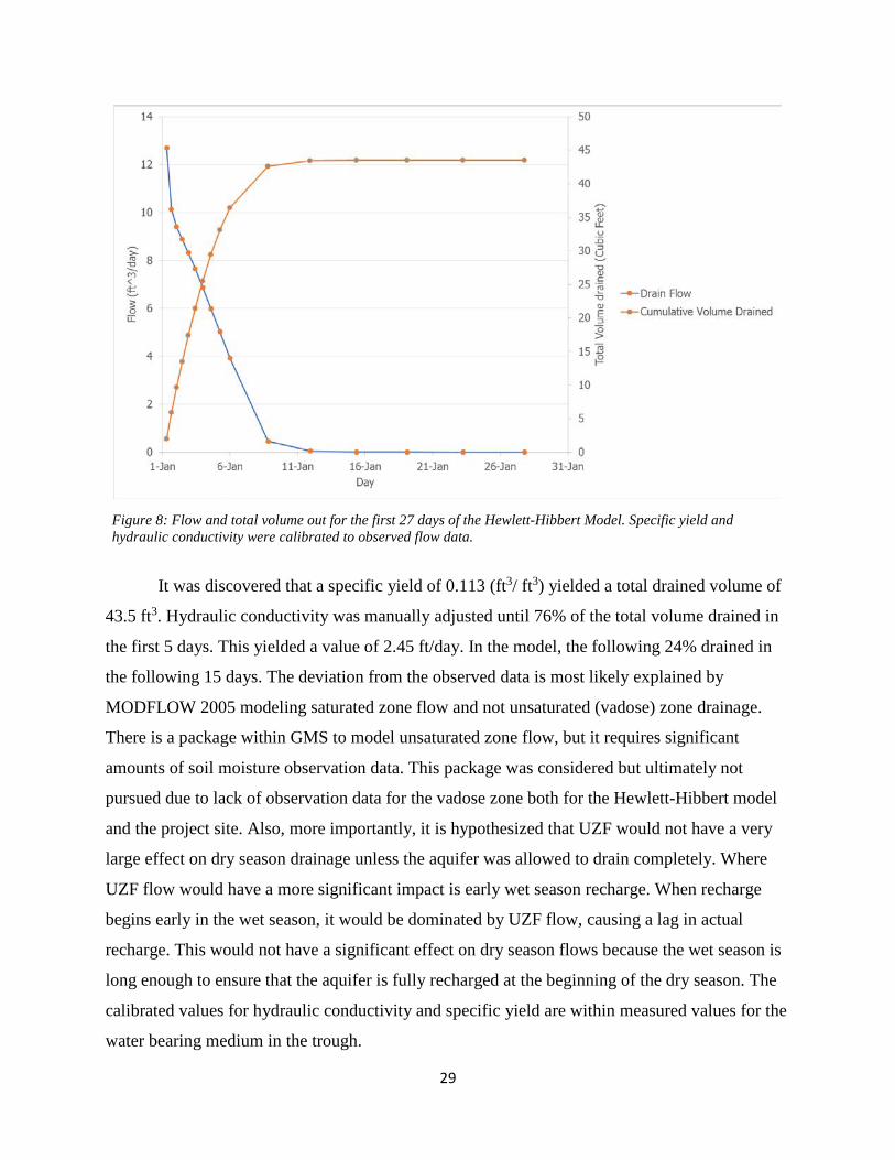
modeled discharge was within the first five days. Figure 8 shows flow over time as well as total

discharge for the first 27 days of the model.

29

Figure 8: Flow and total volume out for the first 27 days of the Hewlett-Hibbert Model. Specific yield and hydraulic conductivity were calibrated to observed flow data.

It was discovered that a specific yield of 0.113 (ft3/ ft3) yielded a total drained volume of

43.5 ft3. Hydraulic conductivity was manually adjusted until 76% of the total volume drained in

the first 5 days. This yielded a value of 2.45 ft/day. In the model, the following 24% drained in

the following 15 days. The deviation from the observed data is most likely explained by

MODFLOW 2005 modeling saturated zone flow and not unsaturated (vadose) zone drainage.

There is a package within GMS to model unsaturated zone flow, but it requires significant

amounts of soil moisture observation data. This package was considered but ultimately not

pursued due to lack of observation data for the vadose zone both for the Hewlett-Hibbert model

and the project site. Also, more importantly, it is hypothesized that UZF would not have a very

large effect on dry season drainage unless the aquifer was allowed to drain completely. Where

UZF flow would have a more significant impact is early wet season recharge. When recharge

begins early in the wet season, it would be dominated by UZF flow, causing a lag in actual

recharge. This would not have a significant effect on dry season flows because the wet season is

long enough to ensure that the aquifer is fully recharged at the beginning of the dry season. The

calibrated values for hydraulic conductivity and specific yield are within measured values for the

water bearing medium in the trough.

30

4.4 Salto Dupi Model Applying what was learned in modeling the Hewlett-Hibbert trough, a model was

constructed and evaluated for the Salto Dupi aquifer. Modeling the Hewlett-Hibbert trough

demonstrated that aquifer characteristics can be estimated when modeling the dewatering of a

sloping aquifer. Spring discharge, hydraulic conductivity, and evapotranspiration were known

and used to calibrate aquifer geometry (aquifer thickness) for the aquifer in Dupi. Two possible

geometries were considered for the Dupi watershed. Scenario one involves a wedge shaped

aquifer where impermeable bedrock remains at a constant elevation while surface topography

elevation increases as it nears the headwaters of the aquifer. Scenario two involves a lens shaped

aquifer where impermeable bedrock mimics surface topography at a constant depth. Figure 9

shows a conceptual model of these two geometries.

31

Figure 9: Side profile view of the wedge and lens model comparing their geometries. Wedge shape geometry was not used as it was compared in another study (VanSickle, 2016).

The wedge shaped geometry is GMS has large amounts of water storage. The modeled

discharge flows at the end of the dry season were high compared to the observed flows. The

author also observed that bedrock streams in the study area have a slope similar to surface

topography, implying that bedrock mimics surface topography. Thus, the lens shape geometry

32

was used for the model because of the author’s bedrock observations in the field. Additionally, a

study was conducted by Jordan VanSickle in a watershed proximal (5km) to the Salto Dupi study

site, comparing different aquifer geometries (lens and wedge shape) and their influence of spring

discharge (VanSickle, 2016). Because of the author’s bedrock observations and VanSickle’s

work regarding the wedge/lens shape comparison, the wedge geometry was not explored in this

study.

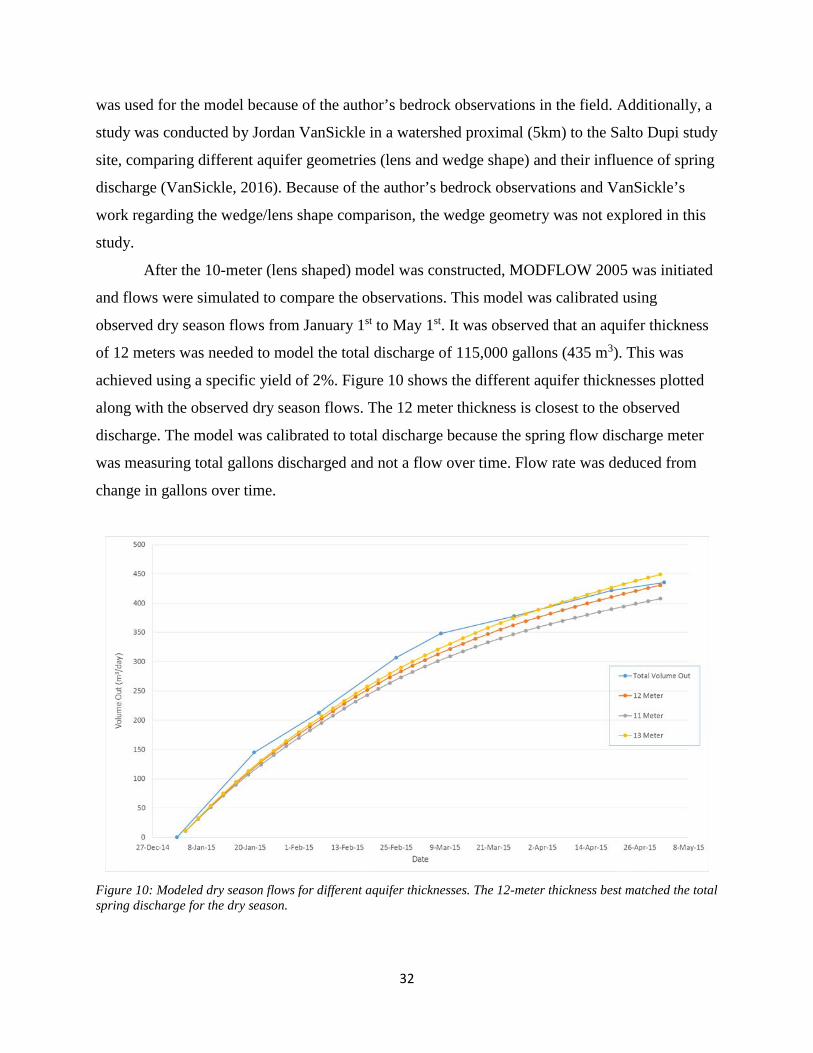
After the 10-meter (lens shaped) model was constructed, MODFLOW 2005 was initiated

and flows were simulated to compare the observations. This model was calibrated using

observed dry season flows from January 1st to May 1st. It was observed that an aquifer thickness

of 12 meters was needed to model the total discharge of 115,000 gallons (435 m3). This was

achieved using a specific yield of 2%. Figure 10 shows the different aquifer thicknesses plotted

along with the observed dry season flows. The 12 meter thickness is closest to the observed

discharge. The model was calibrated to total discharge because the spring flow discharge meter

was measuring total gallons discharged and not a flow over time. Flow rate was deduced from

change in gallons over time.

Figure 10: Modeled dry season flows for different aquifer thicknesses. The 12-meter thickness best matched the total spring discharge for the dry season.

33

Once the aquifer thickness was calibrated to simulate the observed dry season flows,

more stress periods were added along with wet season recharge to model a full-year hydrological

cycle. The dry season was set to begin on December 20th, which was the last day of observed

rainfall in the wet season. The wet season begins on May 1st. Figure 11 shows modeled flow

along with observed data. The model reaches steady-state conditions in the wet season where

recharge is equal to discharge. Flow at this steady state in the wet season is 27.9 m3/day. This

compared closely to the observed flow rate of 26.5 m3/day during the wet season. Flow

drastically decreases at the beginning of the dry season and decreases exponentially as the dry

season continues. The modeled flow on the last day of the dry season 1.34 m3/day. That

compared very well to the observed flow on 1.04 m3/day. This model assumes that recharge is

constant over the wet season, when in reality recharge varies monthly and daily with

precipitation.

Figure 11: Modeled wet and dry season flows for the 12 meter aquifer thickness. Hydraulic conductivity and recharge were specified, and specific yield and aquifer thickness were calibrated to observed flow.

Specific yield and aquifer thickness are the two unknown variables in this model. As

stated before, a specific yield of 2% was used as this is the average value for clays. Then model

thickness was calibrated to the data. The model was calibrated in this way because aquifer

thickness was the greater unknown. A separate model was designed where aquifer thickness was

constant at 10 meters and specific yield was calibrated to observed flow. Not only was the

34

calibration successful, but modeled flow was very similar to that of the thickness calibrated

model. Thus, this model demonstrated non-uniqueness. One could calibrate the model for aquifer

thickness keeping specific yield constant, or one could calibrate for specific yield keeping

thickness constant. Similarly, one could adjust both parameters to model observed flow.

Ultimately, the base flow recession is similar for a model calibrated for thickness or one

calibrated for specific yield. The author estimated that the aquifer thickness was 9-11 meters due

to observations in site. A calibrated aquifer thickness of 12 meters is very plausible for the study

site. The incorporated wet season model modeled peak wet season flows without the author

having to modify and re-adjust ET or runoff. All of these gave credit to the model.

4.5 Climate Scenario Testing

Two different climate scenarios were explored to forecast how changing climate would

affect spring flow. The first was an increase of average monthly temperatures of 3 °C, resulting

in an increased PET of 1.79 meters per year and actual ET of 1.47 meters. Most of this (1.32

meters) was in the wet season, with only 0.14 m in the dry season. After incorporating this into

the water budget, recharge was 0.938 meters for the wet season. This was entered into the model

and flow was simulated. Flow in the wet season was 22.5 m3/day. Flow at the end of the dry

season was 1.06 m3/day.

The second climate scenario was a 10% reduction in precipitation. Rainfall was reduced

to 3.50 meters before runoff and 2.17 meters after runoff. After ET was incorporated, a recharge

of 1.05 meters was entered into the model and flow was simulated. Flow in the wet season was

25.5 m3/day, while flow at the end of the dry season was 1.29 m3/day.

After running these two climate scenarios, a pattern started to emerge. It was observed

that changing the recharge rate had an effect on wet season flows but had little effect on dry

season flows. The model is most sensitive in the wet season flows. In order to estimate how long

it would take for the simulated aquifer to de-water, a simulation was run where the model was

left to drain for one year. After 6 months flow was 0.90 m3/day, and after one year flow was 0.24

m3/day. This showed that spring discharge drastically changes at the beginning of the dry season,

but as the dry season continues, change in flow over time becomes reduced. Figure 12 shows

modeled flow for the climatic scenarios compared to the baseline model.

35

Figure 12: Modeled flow for various climate scenarios

4.6 Impact on the Ngäbe People

The primary goal of this study was to forecast how a changing climate would affect the

local Ngäbe people who depend on these springs for potable water. The author observed that in

the wet season, there is more than enough water for everyone. The study site is a good example.

Wet season flows were in excess of 25 m3/day (6604 gallons/day). For one family this is

sufficient. But, it was also observed that at the end of the dry season flows were around 1 m3/day

(264 gallons). This is roughly 50 gallons a day for a family of five. The model showed that a

changing climate has little effect on late dry season flows and that these flows will be resilient to

climate change.

Forecasting different climate scenarios showed that peak wet season flows were most

sensitive to changes in recharge. This has the potential to affect large scale water distribution

systems in the Comarca. In some small towns, larger spring flow is captured and piped to small

distribution systems. These systems are engineered for peak wet season flows, allowing

community members to receive water from a spigot for 8 months out of the year. During the dry

season, these systems become unusable due to diminishing flows. Community members are then

forced to find their own personal springs to support their family. Diminishing wet season flows

will limit the capacity of these community-scale water distribution systems, making them

unusable for longer periods due to reduced wet season flows. This will ultimately burden family

members because they will have to spend more time collecting water from springs farther away.

36

5.0 Conclusion This study demonstrated that MODFLOW 2005 has the capacity to model steeply

sloping aquifers. The Dupi groundwater model showed non-uniqueness, but ultimately this was

not significant because no one parameter had a significant impact on late dry season spring

discharge. The calibrated Dupi model forecasted that a changing climate will have a large impact

on peak wet season flows and a small impact on late dry season flows. This will impact

community members who receive their water during the wet season from water distribution

systems while having little impact on families who rely on smaller personal springs for their

daily water needs.

6.0 Future Work Opportunities exist for future studies. Soil moisture data could be collected to explore the

unsaturated zone flow of the springs. This would allow the opportunity to quantify how much of

an effect unsaturated zone flow has on small, steeply sloping aquifers. In addition to this, more

climatic data, soil infiltration rates, and spring discharge data could be included to increase the

temporal resolution of the model. More data could be collected on the bedrock geology to deduce

the thickness and geometry of the aquifer. More springs in the area could be modeled, and their

results should be compared to the study site. In addition to more data, other models could be

explored. This includes performing climate scenario testing on a model where specific yield is

calibrated instead of aquifer thickness.

Members of the community were interested in how they could increase the flow of the

springs both in the wet season and the dry season. Community members knew that deforestation

and changing climate were the impetus for reduced spring flow, but to what extent was

unknown. The effect of land cover on spring flow could be explored. One could observe forested

and deforested lands, but also different agricultural crops as well. This would help to show what

could be planted in the watershed to alleviate the effects of climate change. Slash and burn

agriculture is still practiced in the area of study. It would be interesting to study the effect that

burning has on the water budget and spring flow.

37

Works Cited Amoozegar, A. (1989). A Compact Constant-Head Permeameter for Measuring Saturated Hydraulic

Conductivity of the Vadose Zone. Soil Science Society of America Journal Vol. 53 no. 5.

Amoozegar, A. (1989). Comparison of the Glover Solution with the Simultaneous-Equations Approach for Measuring Hydraulic Conductivity. Soil Science Society of America Journal Vol. 53 no. 5.

Aquaveo. (2016). Groundwater Modeling Systems Overview. Retrieved from Aquaveo: http://www.aquaveo.com/software/gms-groundwater-modeling-system-introduction

Coates, A. G., & Obando, J. A. (1996). The Geologis Evolution of the Central American Isthmus. In Evolution and environment in tropical America (pp. 21-56).

Dingman, S. L. (2015). Physical Hydrology. Waveland Press.

ESTESA. (2016). Empresa de Transmision Electrica S.A. Retrieved November 15, 2015, from http://www.hidromet.com.pa/clima_historicos.php?idioma=ing

Fetter, C. W. (2001). Applied Hydrology. Upper Sadle River: Prentice Hall.

Fry, L. (2004). Spring Improvement as a tool for Prevention of Water-related Illness in Four Villages of the Center Province of Cameroon. Houghton, MI: Michigan Technological University.

Hewlett, J. D. (1963). Moisture and energy conditions within a sloping soil mass during drainage. Journal of Geophysical Research 64.8, 1081-1087.

Inchauste, G., & Cancho, C. (2010). Inclusion Social en Panama: la poblacion indigena. 1-44.

Jones, E. K. (2014). IMPROVEMENTS IN SUSTAINABILITY OF GRAVITY-FED WATER SYSTEMS IN THE COMARCA NGÄBE-BUGLÉ, PANAMA: SPRING CAPTURES AND CIRCUIT RIDER MODEL. Houghton, MI: Michigan Technological University.

Magrin, G. O., & Marengo, J. A. (2014). Central and South America In: Climate Change 2014: Impacts, Adaptation, and Vulnerability. Part B: Regional Aspects. Contribution of Working Group II to the Fifth Assessment Report of the Intergovernmental Panel on Climate Change. Climate Change 2014: Impacts, Adaptation, Vulnerability. Part B: Regional Aspects. Contribution of Working Group II to the Fifth Assessment Report of the Intergovernmental Panel on Climate Change, 1499-1566.

McDonald, M. G., & Harbaugh, A. W. (1988). A Modular Three-Dimensional Finite-Difference Ground-Water Flow Model. Virginia: United States Geological Survey .

Molden, D. (2007). Water for food, water for life : a comprehensive assessment of water management in agriculture.

Penman, H. L. (1948). Natural evaporation from open water, bare soil and grass. Proceedings of the Royal Society of London A: Mathematical, Physical and Engineering Sciences (Vol. 193, No. 1032), 120-145.

38

Richard, G. A., Luis, S. P., & Smith, D. R. (1998). Crop evapotranspiration - Guidelines for computing crop water requirements - FAO Irrigation and drainage paper 56. Rome: FAO - Food and Agriculture Organization of the United Nations.

Thornthwaite, C. W. (1948). An Approach toward a Rational Classification of Climate. Geographical Review, 38(1), 55-94.

USDA, U. S. (1986). Urban Hydrology for Small Watersheds. Technical Release 55 (TR-55).

VanSickle, J. (2016). MODELING SPRING CATCHMENT DISCHARGE: A CASE STUDY FOR CANDELA, PANAMA, CENTRAL AMERICA. Houghton, MI: Michigan Technological University.

Zangar, C. N. (1953). Theories and Problems of Water Percolation. Denver, CO: United States Department of the Interior, Bureau of Reclamation.