spring 2013 stat 512 project key project key part 1 (90 ...lfindsen/stat512/projectkey.pdf ·...

Spring 2013 STAT 512 Project Key

1

Project Key Part 1 (90 pts.) due April 18

A reminder – Please do not hand in any unlabeled or unedited SAS output. Include in your write-up only those results that are necessary to present a complete solution (what you want the grader to grade). In particular, questions must be answered in order (including graphs), and all graphs must be fully labeled. Don’t forget to put all necessary information (see course policies) on the first page including names for each group member. Include the SAS input for all questions at the very end of your project; this could be important even though it won’t be graded. This project is concerning the complete analysis using multiple regression of the Real Estate Sales Data set described in Data Set C.7 (APPENC07.DAT). In brief, a city tax assessor is interested in what factors are affecting residential home sale prices. In this project, no interaction terms will be used (until 8.e). Note: there are five qualitative variables in this data set. Three of them are correctly coded: Air conditional, Pool and Highway. Quality has 3 choices so that would be two additional variables, I am calling them qual1 and qual2. Style has possible values of 1 – 11 with no 8 so that is 9 additional variables which I am calling style1 to style10 with no style8. My results reflect this choice of the variables. Because of the length of the project, I will provide the code in a separate file.

1. (4 pts.) The project begins by determining if a multiple regression is appropriate. Remember, if there are qualitative variables with more than two options, you will need to make dummy variables before you run the regression. To perform this step, test the regression relation using all of the explanatory variables. State the hypotheses, test statistic and degrees of freedom, the p-value, the decision and the conclusion in words.

Analysis of Variance

Source DF Sum of Squares

Mean Square

F Value Pr > F

Model 20 8.27019E12 4.135095E11 126.27 <.0001

Error 501 1.640722E12 3274893675

Corrected Total 521 9.910912E12

H0: i = 0 for i = 1, …, 20 Ha: at least one i ≠ 0 for i = 1, …, 20 F = 126.27, df(numerator) = 20, df(denominator) = 501, p-value < 0.0001, decision: reject H0

This data strongly supports that at least one of the predictor variables is important in the regression.


2

2. (7 pts.) The next step is to check the assumptions and look at the original variables. Use all of the “usual plots” (no partial residual plots). It is acceptable to just show the histograms for the explanatory variables. This step does not require any quantitative analysis. (You may use the automated plots generated in SAS.) Be sure to list all of the assumptions and whether they are appropriate or not using the graphs displayed in this step.

Each of the assumptions will be discussed for the individual plots except for Independent Observations which has to be assumed from the experimental data. The results will be summarized at the end.

Original Variables:

Note: I am only going to comment on the non-qualitative variables except if they are so lopsided, that the ‘other’ value is considered an outlier.

right skewed right skewed looks approximately normal

looks approximately normal qualitative looks approximately normal


3

qualitative – maybe outliers left skewed qualitative

qualitative qualitative qualitative


4

qualitative qualitative – maybe outliers qualitative – maybe outliers

qualitative – maybe outliers qualitative qualitative – maybe outliers


5

qualitative – maybe outliers right skewed qualitative – maybe outliers

Conclusion: possible outliers in Xi’s.

Scatterplot:

To make this easier to look at, I have am using the original variables for style and quality. It is hard to see linearity with a qualitative variable so the only thing that can be looked for is outliers


6


7

problems with constant variance with: sqft, bed, bath, year. problems with outliers with: garage, style and maybe bed and bath. To look at linearity, I will regenerate the scatterplot with only quantitative variables:

Possible problems with linearity: bed, bath, year, lot.


8

Residual Plots:


9


10

Comments:

It looks like there is a problem with constant variance in the residual vs. predicted value, sqft, bed, bath, garage, year, some of the style quantitative variables, highway and maybe ac, lot.

I cannot tell if there is a problem with linearity on these plots.

It looks like there is a problem with outliers in the following plots: bed, bath, garage, year. There might be a problem in: predicted value, sq ft, lot. Since there is only one style9 and style10, by definition these are outliers.

Normality plots

From these plots, it looks like there might be a problem with normality of the residuals due to long tails. Note that this might be caused by the outlier problem mentioned above.


11

Conclusion:

linearity: problem constant variance: a problem outliers: a problem normality: a problem independence: assumed

3. (4 pts.) The next step is to look at multicollinearity.

(a) Do the results from the regression indicate that there might be a problem with multicollinearity? Explain your answer. You might need to include additional output from what you displayed in part 1.

This is the output from part 1)


12

Parameter Estimates

Variable DF Parameter Estimate

Standard Error

t Value Pr > |t|

Intercept 1 -2886487 406877 -7.09 <.0001

sqft 1 99.92248 7.61615 13.12 <.0001

bed 1 -4483.24551 3254.24167 -1.38 0.1689

bath 1 10115 4217.24827 2.40 0.0168

ac 1 2164.50354 7938.13709 0.27 0.7852

garage 1 9113.19604 4953.47083 1.84 0.0664

pool 1 12527 10337 1.21 0.2261

year 1 1406.35732 205.61821 6.84 <.0001

qual1 1 143036 14187 10.08 <.0001

qual2 1 10751 8078.28525 1.33 0.1838

style1 1 100125 57955 1.73 0.0847

style2 1 72886 58313 1.25 0.2119

style3 1 85781 58186 1.47 0.1410

style4 1 115098 60575 1.90 0.0580

style5 1 74984 59909 1.25 0.2113

style6 1 94069 59832 1.57 0.1165

style7 1 56874 58344 0.97 0.3301

style9 1 11943 81606 0.15 0.8837

style10 1 13081 83159 0.16 0.8751

lot 1 1.34315 0.23433 5.73 <.0001

highway 1 -35839 17721 -2.02 0.0437

Since at least one of these is significant, we cannot determine if there is a problem with multicollinearity from this data.


13

The two possible methods of testing this are using the SS’s and VIF (Tol). I will show both, though only one of the two

methods is required. Note: VIF is much better than looking at the SS’s

Parameter Estimates


Standard Error

t Value Pr > |t| Type I SS Type II SS Variance Inflation

Intercept 1 -2886487 406877 -7.09 <.0001 4.031153E13 1.648197E11 0

sqft 1 99.92248 7.61615 13.12 <.0001 6.655486E12 5.637065E11 4.66585

bed 1 -4483.24551 3254.24167 -1.38 0.1689 27612564716 6215594105 1.73350

bath 1 10115 4217.24827 2.40 0.0168 1.427102E11 18840321852 3.20420

ac 1 2164.50354 7938.13709 0.27 0.7852 33417146001 243487468 1.40780

garage 1 9113.19604 4953.47083 1.84 0.0664 2.001904E11 11084584306 1.66946

pool 1 12527 10337 1.21 0.2261 123140234 4809893561 1.09352

year 1 1406.35732 205.61821 6.84 <.0001 2.352098E11 1.532023E11 2.09247

qual1 1 143036 14187 10.08 <.0001 6.954309E11 3.328922E11 3.63480

qual2 1 10751 8078.28525 1.33 0.1838 6843097373 5800827317 2.56836

style1 1 100125 57955 1.73 0.0847 76594239754 9774679192 129.50097

style2 1 72886 58313 1.25 0.2119 52624538 5116358792 53.53091

style3 1 85781 58186 1.47 0.1410 15915626022 7117773942 58.05187

style4 1 115098 60575 1.90 0.0580 27618229488 11823303159 12.06533

style5 1 74984 59909 1.25 0.2113 3600622620 5130437942 19.04656

style6 1 94069 59832 1.57 0.1165 28385447805 8095036280 18.99777

style7 1 56874 58344 0.97 0.3301 5066977228 3111930262 104.53207

style9 1 11943 81606 0.15 0.8837 67730682 70140204 2.02964

style10 1 13081 83159 0.16 0.8751 38407398 81030802 2.10759

lot 1 1.34315 0.23433 5.73 <.0001 1.024325E11 1.075968E11 1.19255

highway 1 -35839 17721 -2.02 0.0437 13394228041 13394228041 1.03262


14

From the SS1 and SS2: The predictors which look like they are different are: bed, bath, ac, garage, pool, and the styles.

From VIF: It looks like there is a problem with style1 – style7, remember, there is only one non-zero value for style9 and style10. There might be a problem with sqft.

My conclusion is that the style information is contained in the other data.

(b) Roughly determine which variables (if any) might cause a problem with multicollinearity by looking at the correlations between the explanatory variables both visually (scatterplot) and quantitatively (proc corr). The scatterplot should be repeated from question 2. Which variables do you think might be causing problems? Explain your answer.

Since we are only looking at multicollinearity, I do not need to include the ‘cost’ in the output.

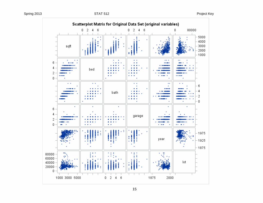
scatterplot:

Since it is very hard to see if qualitative predictors are correlated, I will only included quantitative variables below.


15


16

variable correlation

sqft bed, bath, garage, year, lot

bed sqft, bath, maybe garage, year

bath sqft, bed, year

garage, sqft, bed

year sqft, lot

lot sqft, year

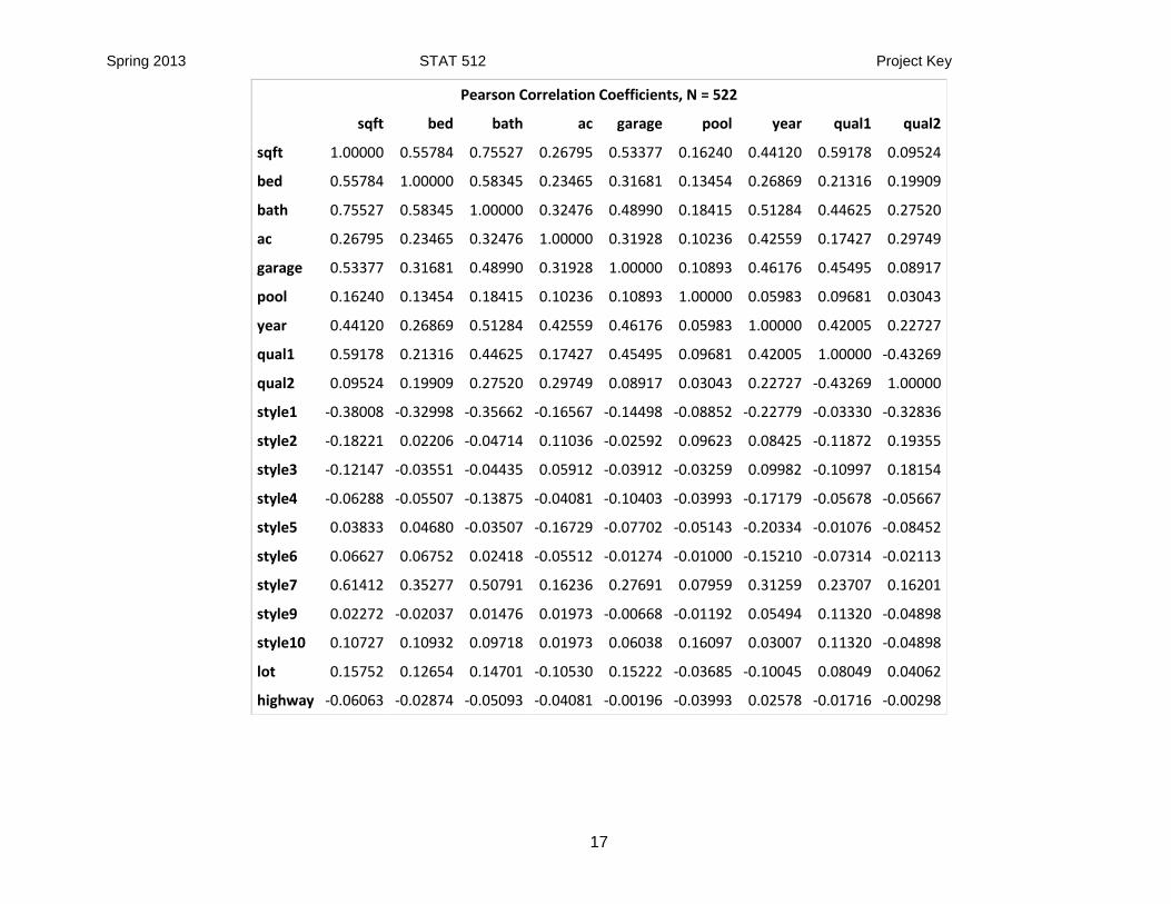
I am including all of the predictor variables in the proc corr.


17

Pearson Correlation Coefficients, N = 522

sqft bed bath ac garage pool year qual1 qual2

sqft 1.00000 0.55784 0.75527 0.26795 0.53377 0.16240 0.44120 0.59178 0.09524

bed 0.55784 1.00000 0.58345 0.23465 0.31681 0.13454 0.26869 0.21316 0.19909

bath 0.75527 0.58345 1.00000 0.32476 0.48990 0.18415 0.51284 0.44625 0.27520

ac 0.26795 0.23465 0.32476 1.00000 0.31928 0.10236 0.42559 0.17427 0.29749

garage 0.53377 0.31681 0.48990 0.31928 1.00000 0.10893 0.46176 0.45495 0.08917

pool 0.16240 0.13454 0.18415 0.10236 0.10893 1.00000 0.05983 0.09681 0.03043

year 0.44120 0.26869 0.51284 0.42559 0.46176 0.05983 1.00000 0.42005 0.22727

qual1 0.59178 0.21316 0.44625 0.17427 0.45495 0.09681 0.42005 1.00000 -0.43269

qual2 0.09524 0.19909 0.27520 0.29749 0.08917 0.03043 0.22727 -0.43269 1.00000

style1 -0.38008 -0.32998 -0.35662 -0.16567 -0.14498 -0.08852 -0.22779 -0.03330 -0.32836

style2 -0.18221 0.02206 -0.04714 0.11036 -0.02592 0.09623 0.08425 -0.11872 0.19355

style3 -0.12147 -0.03551 -0.04435 0.05912 -0.03912 -0.03259 0.09982 -0.10997 0.18154

style4 -0.06288 -0.05507 -0.13875 -0.04081 -0.10403 -0.03993 -0.17179 -0.05678 -0.05667

style5 0.03833 0.04680 -0.03507 -0.16729 -0.07702 -0.05143 -0.20334 -0.01076 -0.08452

style6 0.06627 0.06752 0.02418 -0.05512 -0.01274 -0.01000 -0.15210 -0.07314 -0.02113

style7 0.61412 0.35277 0.50791 0.16236 0.27691 0.07959 0.31259 0.23707 0.16201

style9 0.02272 -0.02037 0.01476 0.01973 -0.00668 -0.01192 0.05494 0.11320 -0.04898

style10 0.10727 0.10932 0.09718 0.01973 0.06038 0.16097 0.03007 0.11320 -0.04898

lot 0.15752 0.12654 0.14701 -0.10530 0.15222 -0.03685 -0.10045 0.08049 0.04062

highway -0.06063 -0.02874 -0.05093 -0.04081 -0.00196 -0.03993 0.02578 -0.01716 -0.00298


18


style1 style2 style3 style4 style5 style6 style7 style9 style10 lot highway

sqft -0.38008 -0.18221 -0.12147 -0.06288 0.03833 0.06627 0.61412 0.02272 0.10727 0.15752 -0.06063

bed -0.32998 0.02206 -0.03551 -0.05507 0.04680 0.06752 0.35277 -0.02037 0.10932 0.12654 -0.02874

bath -0.35662 -0.04714 -0.04435 -0.13875 -0.03507 0.02418 0.50791 0.01476 0.09718 0.14701 -0.05093

ac -0.16567 0.11036 0.05912 -0.04081 -0.16729 -0.05512 0.16236 0.01973 0.01973 -0.10530 -0.04081

garage -0.14498 -0.02592 -0.03912 -0.10403 -0.07702 -0.01274 0.27691 -0.00668 0.06038 0.15222 -0.00196

pool -0.08852 0.09623 -0.03259 -0.03993 -0.05143 -0.01000 0.07959 -0.01192 0.16097 -0.03685 -0.03993

year -0.22779 0.08425 0.09982 -0.17179 -0.20334 -0.15210 0.31259 0.05494 0.03007 -0.10045 0.02578

qual1 -0.03330 -0.11872 -0.10997 -0.05678 -0.01076 -0.07314 0.23707 0.11320 0.11320 0.08049 -0.01716

qual2 -0.32836 0.19355 0.18154 -0.05667 -0.08452 -0.02113 0.16201 -0.04898 -0.04898 0.04062 -0.00298

style1 1.00000 -0.29470 -0.31159 -0.12230 -0.15753 -0.15753 -0.49477 -0.03652 -0.03652 0.07336 0.12178

style2 -0.29470 1.00000 -0.13216 -0.05187 -0.06682 -0.06682 -0.20986 -0.01549 -0.01549 -0.07117 -0.00943

style3 -0.31159 -0.13216 1.00000 -0.05485 -0.07064 -0.07064 -0.22189 -0.01638 -0.01638 -0.08161 -0.01418

style4 -0.12230 -0.05187 -0.05485 1.00000 -0.02773 -0.02773 -0.08709 -0.00643 -0.00643 0.00480 -0.02153

style5 -0.15753 -0.06682 -0.07064 -0.02773 1.00000 -0.03571 -0.11218 -0.00828 -0.00828 0.06192 -0.02773

style6 -0.15753 -0.06682 -0.07064 -0.02773 -0.03571 1.00000 -0.11218 -0.00828 -0.00828 0.06818 -0.02773

style7 -0.49477 -0.20986 -0.22189 -0.08709 -0.11218 -0.11218 1.00000 -0.02601 -0.02601 -0.02657 -0.08709

style9 -0.03652 -0.01549 -0.01638 -0.00643 -0.00828 -0.00828 -0.02601 1.00000 -0.00192 0.00153 -0.00643

style10 -0.03652 -0.01549 -0.01638 -0.00643 -0.00828 -0.00828 -0.02601 -0.00192 1.00000 -0.00291 -0.00643

lot 0.07336 -0.07117 -0.08161 0.00480 0.06192 0.06818 -0.02657 0.00153 -0.00291 1.00000 0.07845

highway 0.12178 -0.00943 -0.01418 -0.02153 -0.02773 -0.02773 -0.08709 -0.00643 -0.00643 0.07845 1.00000

I used an arbitrary cutoff of 0.5 to determine correlation.


19

variable correlation

sqft bed, bath, garage, qual1, style7

bed sqft, bath

bath sqft, bed, year, style7

garage sqft

year bath, quality

qual1 sqft

style7 sqft, bath

not correlated: ac, pool, qual2, stylei (i ≠ 7), lot, highway

(c) Is your analysis consistent in parts a) and b)? Explain your answer.

Some of the correlations are the same and some are different. In general, it looks like sqft, bed, bath, year and garage are correlated. The only qualitative variables that are correlated are qual1 (high quality) and style7.

4. (11.5 pts.) Before we run model selection, it is a good idea to make some predictions on which variables might be included in the final model.

(a) From the regression analysis, which variables do you think might be important in the final model. Explain your answer.


20

Parameter Estimates


Standard Error

t Value Pr > |t|

Intercept 1 -2886487 406877 -7.09 <.0001

sqft 1 99.92248 7.61615 13.12 <.0001

bed 1 -4483.24551 3254.24167 -1.38 0.1689

bath 1 10115 4217.24827 2.40 0.0168

ac 1 2164.50354 7938.13709 0.27 0.7852

garage 1 9113.19604 4953.47083 1.84 0.0664

pool 1 12527 10337 1.21 0.2261

year 1 1406.35732 205.61821 6.84 <.0001

qual1 1 143036 14187 10.08 <.0001

qual2 1 10751 8078.28525 1.33 0.1838

style1 1 100125 57955 1.73 0.0847

style2 1 72886 58313 1.25 0.2119

style3 1 85781 58186 1.47 0.1410

style4 1 115098 60575 1.90 0.0580

style5 1 74984 59909 1.25 0.2113

style6 1 94069 59832 1.57 0.1165

style7 1 56874 58344 0.97 0.3301

style9 1 11943 81606 0.15 0.8837

style10 1 13081 83159 0.16 0.8751

lot 1 1.34315 0.23433 5.73 <.0001

highway 1 -35839 17721 -2.02 0.0437

The predictor variables that have low P-values are: sqft, bath, garage (maybe), year, qual1, style1 (maybe), style4 (maybe), lot and highway.


21

(b) Which variables do you think might be important by looking at the correlations between the sales price and each of the explanatory variables. Your SAS output should include both a visual representation (scatterplot) and quantitative data (proc corr). Which variables do you think should be included in the final model and which variables do you think might be dropped. Explain your answer.


22

From the scatterplot: sqft, bed, bath, ac (maybe), pool (maybe), year (looks quadratic), and lot are correlated, therefore quality (can’t tell), style (can’t tell) and highway (looks like outliers) should be dropped. It is difficult to tell if a qualitative variable is correlated using this method.


sqft bed bath ac garage pool year qual1 qual2

cost 0.81947 0.41332 0.68369 0.28860 0.57779 0.14661 0.55552 0.74632 -0.03349


style1 style2 style3 style4 style5 style6 style7 style9 style10 lot highway

cost -0.17866 -0.14849 -0.08102 -0.06423 -0.03625 0.00323 0.39308 0.03851 0.08648 0.22417 -0.05097

It looks like sqft, bed (maybe), bath, garage, year, qual1 are correlated, therefore ac, pool, qual2, styles, lot and highway should be dropped.

(c) Generate partial regression plots (it is extremely useful to have the best fit line on the plot). Which variables do you think should be included in the final model. Explain your answer. Please comment on each of the plots.


23

sqft: definitely significant

bed: might or might not be significant especially since the cost goes down as the number of bedrooms increases.

bath: might or might not be significant but more likely

ac: not significant

garage: might or might not be significant


24

pool: probably not significant

year: significant

qual1 significant

qual2: not significant

style1, style2: curve due to outliers


25

style3, style4, style5, style6, style7, style9: curve due to outliers


26

style10: curve due to outliers

lot: significant or is there a problem with outliers

highway: might be significant, is the curve due to outliers?

(d) Compare the methods used in parts a), b) and c). Are the results the same? different? Which variables do you think should be included in the final model?

procedure significance

t-tests sqft, bed, garage, year, qual1, style1, style4, lot, highway

scatterplot sqrt, bed, bath, ac, pool, year, lot

proc corr sqrt, bed, bath, garage, year, qual1

partial residual plots sqrt, bath, garage, year, qual1, lot, highway

The results are generally the same. Remember that I did not include any qualitative variables from the scatterplot. From the above information, I would expect sqft, bed or bath, garage, year, qual1, lot and highway to be in the final model. There is a possibility of both bed and bath and some of the style dummy variables.

(e) Does multicollinearity (question 3) affect your answer in part d)? Explain your answer.

Multicollinearity could be a problem. From the VIF’s, it shows that the style dummy variables are correlated with the other variables so that could be a problem. From the SS, bed, bath, garage and year might also have difficulties. The pairwise correlations might be showing some problems here also since sqft should be included in the model and it is correlated with bed, bath, garage, year and lot.


27

5. (9.5 pts.) In this step, we will run the model selection. Remember, the best model has the least number of explanatory variables that can adequately predict the response variable.

(a) Determine the three best regression models using the Cp criterion. Summarize your results (include the explanatory

variables but not their values, and values of R2, adjusted R2 and Cp). Explain your answer.

Note: I am including at least one model from each number of predictor variables and all models that are included elsewhere in

the discussion.

Number in

Model

R-Square

Adjusted R-

Square

C(p) C(p)-p Variables in Model

1 0.6715 0.6709 476.0554 474.0554 sqft

2 0.7767 0.7758 159.8867 156.8867 sqft qual1

3 0.7987 0.7976 95.1274 91.1274 sqft year qual1

4 0.8163 0.8149 43.8837 38.8837 sqft year qual1 lot

5 0.8219 0.8201 29.1254 23.1254 sqft year qual1 style7 lot

6 0.8240 0.8220 24.5500 17.55 sqft bath year qual1 style7 lot

7 0.8265 0.8242 18.9857 10.9857 sqft bath year qual1 style1 style7 lot

8 0.8279 0.8253 16.7104 7.7104 sqft bath year qual1 style1 style7 lot highway

9 0.8293 0.8263 14.4585 4.4585 sqft bath garage year qual1 style1 style7 lot highway

9 0.8291 0.8261 15.1777 5.1777 sqft bath garage year qual1 style1 style4 style7 lot

9 0.8290 0.8260 15.3771 5.3771 sqft bath year qual1 style1 style4 style7 lot highway

10 0.8305 0.8272 12.9165 1.9165 sqft bath garage year qual1 style1 style4 style7 lot highway

10 0.8300 0.8267 14.4116 3.4116 sqft bed bath garage year qual1 style1 style7 lot highway

10 0.8299 0.8266 14.6932 3.6932 sqft bath garage year qual1 qual2 style1 style7 lot highway

11 0.8312 0.8275 12.9451 0.9451 sqft bed bath garage year qual1 style1 style4 style7 lot highway

11 0.8311 0.8275 13.0154 1.0154 sqft bath garage year qual1 qual2 style1 style4 style7 lot highway

11 0.8311 0.8274 13.2381 1.2381 sqft bath garage year qual1 style1 style3 style4 style7 lot highway

12 0.8317 0.8278 13.2255 0.2255 sqft bath garage year qual1 style1 style2 style3 style4 style6 lot highway


28

12 0.8317 0.8278 13.2438 0.2438 sqft bed bath garage year qual1 qual2 style1 style4 style7 lot highway

12 0.8317 0.8277 13.4624 0.4624 sqft bed bath garage year qual1 style1 style3 style4 style7 lot highway

13 0.8324 0.8281 13.3098 -0.6902 sqft bath garage year qual1 qual2 style1 style2 style3 style4 style6 lot highway

14 0.8329 0.8282 13.8076 -1.1924 sqft bed bath garage year qual1 qual2 style1 style2 style3 style4 style6 lot highway

15 0.8333 0.8284 14.4061 -1.5939 sqft bath garage year qual1 qual2 style1 style2 style3 style4 style5 style6 style7 lot highway

16 0.8339 0.8286 14.6421 -2.3579 sqft bed bath garage year qual1 qual2 style1 style2 style3 style4 style5 style6 style7 lot highway

17 0.8344 0.8288 15.1033 -2.8967 sqft bed bath garage pool year qual1 qual2 style1 style2 style3 style4 style5 style6 style7 lot highway

18 0.8344 0.8285 17.0308 -1.9692 sqft bed bath ac garage pool year qual1 qual2 style1 style2 style3 style4 style5 style6 style7 lot highway

19 0.8344 0.8282 19.0214 -0.9786 sqft bed bath ac garage pool year qual1 qual2 style1 style2 style3 style4 style5 style6 style7 style10 lot highway

20 0.8345 0.8278 21.0000 0 sqft bed bath ac garage pool year qual1 qual2 style1 style2 style3 style4 style5 style6 style7 style9 style10 lot highway

Model # of variables Cp adjusted R2 R2 predictors

AA 12 13.2255 0.8278 0.8317 sqft bath garage year qual1 style1 style2 style3 style4 style6 lot highway

B 12 13.2438 0.8278 0.8317 sqft bed bath garage year qual1 qual2 style1 style4 style7 lot highway

C 12 13.4624 0.8277 0.8317 sqft bed bath garage year qual1 style1 style3 style4 style7 lot highway

D 10 12.9165 0.8272 0.8305 sqft bath garage year qual1 style1 style4 style7 lot highway E 11 12.9451 0.8271 0.8312 sqft bed bath garage year qual1 style1 style4 style7 lot highway

F 11 0.8271 0.8307 sqft bath garage year qual1 style1 style3 style4 style6 lot highway

G 9 14.4585 0.8263 0.8293 sqft bath garage year qual1 style1 style7 lot highway

The answer to part a are the green models. I choose them because they had CP’s closest to the number of parameters which

is the number of predictors in the model + 1. To help me with my answer, I placed an extra column in the SAS output above.

(b) Determine the best regression method using each of the automatic methods, forward stepwise regression, forward

selection and backward elimination. Again just include the explanatory variables for each of them. Are these models

the same or different from each other and of the models chosen in part a)?


29

forward stepwise

Summary of Stepwise Selection

Step Variable Entered

Variable Removed

Number Vars In

Partial R-Square

Model R-Square

C(p) F Value Pr > F

1 sqft 1 0.6715 0.6715 476.055 1063.10 <.0001

2 qual1 2 0.1051 0.7767 159.887 244.32 <.0001

3 year 3 0.0221 0.7987 95.1274 56.77 <.0001

4 lot 4 0.0176 0.8163 43.8837 49.52 <.0001

5 style7 5 0.0055 0.8219 29.1254 16.04 <.0001

6 bath 6 0.0022 0.8240 24.5500 6.36 0.0120

7 style1 7 0.0025 0.8265 18.9857 7.41 0.0067

8 highway 8 0.0014 0.8279 16.7104 4.21 0.0406

9 garage 9 0.0014 0.8293 14.4585 4.22 0.0406

10 style4 10 0.0012 0.8305 12.9165 3.53 0.0609

This is model D above.


30

forward selection

Summary of Forward Selection

Step Variable Entered

Number Vars In

Partial R-Square

Model R-Square

C(p) F Value Pr > F

1 sqft 1 0.6715 0.6715 476.055 1063.10 <.0001

2 qual1 2 0.1051 0.7767 159.887 244.32 <.0001

3 year 3 0.0221 0.7987 95.1274 56.77 <.0001

4 lot 4 0.0176 0.8163 43.8837 49.52 <.0001

5 style7 5 0.0055 0.8219 29.1254 16.04 <.0001

6 bath 6 0.0022 0.8240 24.5500 6.36 0.0120

7 style1 7 0.0025 0.8265 18.9857 7.41 0.0067

8 highway 8 0.0014 0.8279 16.7104 4.21 0.0406

9 garage 9 0.0014 0.8293 14.4585 4.22 0.0406

10 style4 10 0.0012 0.8305 12.9165 3.53 0.0609

11 bed 11 0.0007 0.8312 12.9451 1.97 0.1613

12 qual2 12 0.0006 0.8317 13.2438 1.70 0.1928

13 style9 13 0.0004 0.8322 13.9149 1.33 0.2495

14 style3 14 0.0004 0.8325 14.7781 1.14 0.2867

15 style6 15 0.0006 0.8331 14.9437 1.84 0.1758

16 pool 16 0.0004 0.8336 15.7143 1.23 0.2674

17 style10 17 0.0004 0.8339 16.6540 1.06 0.3030

This is not listed in the above table and it has too many parameters so it will not be considered.


31

backward elimination

Variable Parameter Estimate

Standard Error

Type II SS F Value Pr > F

Intercept -2872765 369207 1.983577E11 60.54 <.0001

sqft 100.26719 7.20755 6.340619E11 193.53 <.0001

bath 10431 3867.64533 23829565134 7.27 0.0072

garage 9944.21164 4890.66967 13545454701 4.13 0.0425

year 1424.24280 190.00471 1.840894E11 56.19 <.0001

qual1 131339 10025 5.623093E11 171.63 <.0001

style1 41991 7966.28882 91030027055 27.78 <.0001

style2 17832 10251 9914528711 3.03 0.0825

style3 29965 9616.04294 31814945318 9.71 0.0019

style4 55669 18722 28966610963 8.84 0.0031

style6 32452 14634 16112117938 4.92 0.0270

lot 1.34206 0.22887 1.126605E11 34.39 <.0001

highway -36422 17700 13872192851 4.23 0.0401

This is model A above.

(c) Normally, what we would do is to perform the rest of the project on each of the best models and then determine which model is the best at the end. However, to save time, we will choose the best model first and then only perform diagnostics and remedial actions on that one model.

i. Run a linear regression on each of the best methods from parts a) and b). If necessary, run a manual backwards elimination and repeat the calculation. (p-values of close to 0.05 are still acceptable.) Give the equation of the fitted regression line for your final model. Explain your choice.

A problem occurs because both of the predictors with multiple dummy variables, quality and style are in the final selection. However, it does make sense to not include all of possible permutations. If qual1 is in the model and qual2 is not in the model, that just means that low and medium quality are treated the same. The problem is more complicated with style since we don’t know what each of the choices stands for. However, we do not have to include all of the choices, because the ones not included are not relevant to the final sales price.


32

To run this part, start off with the models with the most predictors and see if they reduce to the ones with lower numbers of predictors.

Note: I am labeling all of my models with letters. If they are on the table above, they will be in grey. I am also not including the adjusted R2 below, because all of the data is in the table above.

Model A

Parameter Estimates


Standard Error

t Value Pr > |t|

Intercept 1 -2872765 369207 -7.78 <.0001

sqft 1 100.26719 7.20755 13.91 <.0001

bath 1 10431 3867.64533 2.70 0.0072

garage 1 9944.21164 4890.66967 2.03 0.0425

year 1 1424.24280 190.00471 7.50 <.0001

qual1 1 131339 10025 13.10 <.0001

style1 1 41991 7966.28882 5.27 <.0001

style2 1 17832 10251 1.74 0.0825

style3 1 29965 9616.04294 3.12 0.0019

style4 1 55669 18722 2.97 0.0031

style6 1 32452 14634 2.22 0.0270

lot 1 1.34206 0.22887 5.86 <.0001

highway 1 -36422 17700 -2.06 0.0401

In this model nothing should be removed. The largest p-value is 0.0825 which is for style2. See below for what happens when this parameter is removed.


33

Model B

Parameter Estimates


Standard Error

t Value Pr > |t|

Intercept 1 -2762411 381771 -7.24 <.0001

sqft 1 101.74278 7.21604 14.10 <.0001

bed 1 -4264.55579 3204.76883 -1.33 0.1839

bath 1 10671 4193.19909 2.54 0.0112

garage 1 9860.01871 4902.02032 2.01 0.0448

year 1 1382.08473 195.39018 7.07 <.0001

qual1 1 138635 13781 10.06 <.0001

qual2 1 10015 7679.68857 1.30 0.1928

style1 1 20664 6446.52641 3.21 0.0014

style4 1 34635 18265 1.90 0.0585

style7 1 -23497 7998.56259 -2.94 0.0035

lot 1 1.30690 0.23057 5.67 <.0001

highway 1 -36294 17706 -2.05 0.0409

In this model, qual2 should be removed first because it has the highest p-value. This is Model E.


34

Model C

Parameter Estimates


Standard Error

t Value Pr > |t|

Intercept 1 -2871904 362734 -7.92 <.0001

sqft 1 103.16223 7.16051 14.41 <.0001

bed 1 -4270.05951 3205.89622 -1.33 0.1835

bath 1 12192 4031.68811 3.02 0.0026

garage 1 10488 4881.91382 2.15 0.0322

year 1 1434.82774 186.08733 7.71 <.0001

qual1 1 126925 10179 12.47 <.0001

style1 1 23473 7311.96443 3.21 0.0014

style3 1 11401 9367.36243 1.22 0.2241

style4 1 38008 18559 2.05 0.0411

style7 1 -20157 8740.23561 -2.31 0.0215

lot 1 1.34052 0.22966 5.84 <.0001

highway 1 -36087 17708 -2.04 0.0421

In this model, style3 should be removed first because it has the highest p-value. This is again Model E.


35

Model E

Parameter Estimates


Standard Error

t Value Pr > |t|

Intercept 1 -2929927 359757 -8.14 <.0001

sqft 1 102.94627 7.16169 14.37 <.0001

bed 1 -4491.99679 3202.21622 -1.40 0.1613

bath 1 12178 4033.57340 3.02 0.0027

garage 1 10454 4884.13900 2.14 0.0328

year 1 1467.38746 184.24128 7.96 <.0001

qual1 1 126509 10178 12.43 <.0001

style1 1 18997 6322.88921 3.00 0.0028

style4 1 33986 18271 1.86 0.0634

style7 1 -24552 7963.02914 -3.08 0.0022

lot 1 1.33491 0.22972 5.81 <.0001

highway 1 -36045 17717 -2.03 0.0424

In this model, bed should be removed first because it has the highest p-value. This is again Model D.


36

Model D

Parameter Estimates


Standard Error

t Value Pr > |t|

Intercept 1 -2952236 359746 -8.21 <.0001

sqft 1 100.52514 6.95718 14.45 <.0001

bath 1 10581 3873.20977 2.73 0.0065

garage 1 10303 4887.57339 2.11 0.0355

year 1 1475.54739 184.32372 8.01 <.0001

qual1 1 128682 10069 12.78 <.0001

style1 1 19984 6289.59900 3.18 0.0016

style4 1 34351 18287 1.88 0.0609

style7 1 -23737 7949.34070 -2.99 0.0030

lot 1 1.32585 0.22985 5.77 <.0001

highway 1 -36531 17730 -2.06 0.0399

The P-value for style4 is a little high, but nothing should be removed.

The final models that I obtained for models A and D which are the two models that were obtained by the automatic methods. I would choose D because it has fewer parameters even though model A has less bias (CP is closer to p).

I am going to continue the backward elimination process on models A and D until there are no further p-values higher than 0.05 for your information even though my final answer is above.


37

Model F (generated from model A by removing style2)

Parameter Estimates


Standard Error

t Value Pr > |t|

Intercept 1 -2946930 367465 -8.02 <.0001

sqft 1 94.95758 6.54232 14.51 <.0001

bath 1 10575 3874.42339 2.73 0.0066

garage 1 10593 4886.10977 2.17 0.0306

year 1 1470.00925 188.54786 7.80 <.0001

qual1 1 132634 10018 13.24 <.0001

style1 1 34246 6619.01497 5.17 <.0001

style3 1 22414 8597.43989 2.61 0.0094

style4 1 49248 18391 2.68 0.0077

style6 1 28145 14452 1.95 0.0520

lot 1 1.36633 0.22889 5.97 <.0001

highway 1 -35873 17733 -2.02 0.0436

This model was not generated in part a), however, the CP value witll be greater than 13.2381 so the difference will be greater than 1.2381 and so it is probability not the best model.


38

Model G (generated from Model D by removing style4)

Parameter Estimates


Standard Error

t Value Pr > |t|

Intercept 1 -2865457 357647 -8.01 <.0001

sqft 1 101.27161 6.96296 14.54 <.0001

bath 1 9798.35842 3860.26032 2.54 0.0114

garage 1 10056 4897.84752 2.05 0.0406

year 1 1432.88644 183.37049 7.81 <.0001

qual1 1 129561 10083 12.85 <.0001

style1 1 17433 6156.49251 2.83 0.0048

style7 1 -25430 7917.57022 -3.21 0.0014

lot 1 1.33104 0.23040 5.78 <.0001

highway 1 -36594 17774 -2.06 0.0400

There are no p-values here above 0.05.

Even though a better answer would be model D, I am going to complete the analysis using model G because more students would choose this model. Model D is better even though it has one more predictor because the CP value is closer to p so the answer is less biased. The Adjusted R2 are approximately the same.

Final Model: Yi = β0 + β1 sqft + β2 bath + β3 garage + β4 year + β5 qual1 + β6 style1 + β7 style7 + β8 lot + β9 highway


39

Even though it is not required, I am including the complete output from model G:



Mean Square

F Value Pr > F

Model 9 8.219565E12 9.13285E11 276.47 <.0001

Error 512 1.691347E12 3303411517


Root MSE 57475 R-Square 0.8293

Dependent Mean 277894 Adj R-Sq 0.8263

Coeff Var 20.68245

Parameter Estimates


Standard Error

t Value Pr > |t|

Intercept 1 -2865457 357647 -8.01 <.0001

sqft 1 101.27161 6.96296 14.54 <.0001

bath 1 9798.35842 3860.26032 2.54 0.0114

garage 1 10056 4897.84752 2.05 0.0406

year 1 1432.88644 183.37049 7.81 <.0001

qual1 1 129561 10083 12.85 <.0001

style1 1 17433 6156.49251 2.83 0.0048

style7 1 -25430 7917.57022 -3.21 0.0014

lot 1 1.33104 0.23040 5.78 <.0001

highway 1 -36594 17774 -2.06 0.0400


40

ii. Is your answer in part i) consistent with the results from questions 3 and 4? Do you expect a problem with multicollinearity?

From questions 4, I expected to have sqft, bed or bath, garage, year, qual1, lot and highway. I was not sure about the style dummy variables. Therefore, the previous model is consistent with what was stated before. From question 3, I would expect some problem with multicollinearity because a) style7 has a large VIF and it was not certain which variables this was correlated with and b) sqft, bath, garage, year and lot showed some problems with pairwise correlation.

6. (28 pts.) We are now going to check our assumptions on the best model obtained in Step 5. For ease in grading, I am splitting your answer into the type of information that you are checking. Each assumption will be addressed in at least one (normally more than one) of the parts. Please comment on all graphs shown and write at least one sentence of conclusion for each part. We have already looked at the original variables and the scatterplots between them so you do not need to repeat that here.

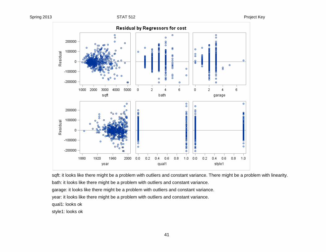
(a) residual plots.

predicted value: there is a problem with constant variance and might be a problem with outliers. It is hard to determine if there is a problem with linearity.


41

sqft: it looks like there might be a problem with outliers and constant variance. There might be a problem with linearity.

bath: it looks like there might be a problem with outliers and constant variance.

garage: it looks like there might be a problem with outliers and constant variance.

year: it looks like there might be a problem with outliers and constant variance.

qual1: looks ok

style1: looks ok


42

style7: looks ok

lot: there might be a problem with outliers, I am not sure about constant variance.

highway: There is a problem with constant variance; are the points at highway=1, outliers?

(b) normality plots.

normality still looks like there is a problem with too long tails which might be due to outliers.


43

(c) partial regression plots.

sqft: this is definitely significant and it looks like there is a problem with outliers since the fitted line doesn’t look like it goes through the points.

bath: this is significant and again there is a problem with the outliers.

garage: this is significant and again there is a problem with the outliers.

year: this is significant and again there is a problem with the outliers. It also looks like there is some curvature.

qual1: this is significant and again there is a problem with the outliers in this case, the best line isn’t close to going through the line of the majority of the points.


44

style1: this doesn’t look significant if you ignore the outliers.

style7: this looks like it might be significant.

lot: this is significant and again there is a problem with the outliers.

highway: this is hard to tell because of the small number of points at 1.


45

(d) qualitative (quantitative) outlier and influential points (Note: this is considered a large data set). Be sure to include your results from looking at the interactive scatterplot. Do not consider non-outliers as being influential.

type element cutoff

Y outliers RStudent tn-p-1(1 -

) = t522-9-1(1 –

) = t512(1 – 4.79 x 10-5) = 3.93214

X outliers hat diagonal element

= 0.03831

influential DFFITS

= 0.2768

influential Cook’s Distance

Fp,n-p (50th percentile) = F10,522-10 (50th) = F10,512 (50th) = 0.93541

Influential DFBETAS

= 0.08763

influential variance COV RATIO

Because of the large number of outliers and influential points in this project, I am only going to list the problem points for each of the above types. I did my analysis using Excel by first copying the matrix to a word document and then copying the table into Excel. I then repeatedly used the sort function to find the points that were outside of each of the above cutoffs. After I identified each of the outliers, I then looked at the interactive scatterplot to determine if I thought they were outliers. Both of the Y outliers were really outliers. For the X outliers, the observations that I did not consider outliers have a ‘no’ in parentheses after the number. For the observations that I thought were outliers, I indicated which predictors, the observation was an outlier for.


46

type problem points

Y outliers 72, 73

X outliers 6 (garage), 25 (no), 37 (no), 49 (no), 50 (no), 52 (no), 55 (year), 56 (lot), 58 (no), 59 (no), 60 (no), 61 (no), 62 (no), 63 (lot), 64 (no), 65 (no), 66 (no), 67 (no), 68 (lot), 81 (many), 96 (year, lot), 103 (sqft), 104 (sqft, bath, lot), 108 (bath), 120 (bath), 123 (lot), 132 (no), 146 (year?), 148 (year), 155 (sqft, year), 161 (garage), 177 (lot), 201 (bath), 203 (sqft, year, lot), 211 (year), 241 (lot), 314 (lot), 344 (no), 466 (lot), 511 (no) (note: it considered all points with highway = 1 as outliers so none were included here)

Outliers to be considered:

6, 55, 56, 68, 72, 73, 81, 96, 103, 104, 108, 120, 123, 146, 148, 155, 161, 177, 201 203, 211, 241, 314, 466


47

In the following table, I only included the outliers to be considered and I have highlighted the influential points.

(e) multicollinearity including visual (scatter plots), pairwise correlation and quantitative information.

Note: this information is the same as in Question 3 but with fewer variables so it should be easier to tell what is happening.

Obs Cook's

D Cov

Ratio DFFITS

DFBETA

Intercept sqft bath garage year qual1 style1 style7 lot highway

6 0.003 1.0902 -0.1678 -0.0293 0.0358 -0.0164 -0.1569 0.0317 0.0373 -0.031 0.0004 0.0358 0.0078

55 0 1.0996 -0.0435 -0.0372 0.0008 0.0005 -0.0089 0.0372 -0.006 0.0052 -0.0147 -0.0036 -0.0024

56 0.001 1.065 -0.0871 0.0192 0.0161 -0.0229 -0.0148 -0.0178 0.0202 -0.0204 0.0022 -0.0659 0.0123

68 0.014 1.1392 -0.372 -0.0013 -0.0332 0.0894 0.002 0.0028 0.0052 0.0023 -0.0285 -0.1601 -0.3

72 0.033 0.7354 0.5846 -0.0518 0.122 -0.1528 -0.0109 0.0498 0.288 -0.0425 0.1174 0.0457 -0.0041

73 0.073 0.683 0.871 -0.1553 0.2937 0.1979 -0.1134 0.1399 0.1396 0.2987 -0.3862 0.004 -0.0708

81 0.001 1.1841 0.0732 0.0106 0.0101 -0.0039 0.0591 -0.0126 -0.0068 0.0095 -0.016 0.0072 -0.0038

96 0.086 0.9521 0.9326 0.3247 -0.2565 0.1316 -0.0962 -0.323 0.5143 -0.0228 0.0868 0.643 -0.0563

103 0.096 0.8257 -0.9935 0.1265 -0.7929 0.6489 0.0732 -0.1143 -0.0127 -0.024 0.1035 0.0968 -0.0038

104 0.061 0.812 -0.7877 -0.001 -0.3071 -0.0955 0.1831 0.0161 -0.086 -0.0322 0.0703 -0.3351 0.019

108 0.022 1.029 0.4705 -0.1752 0.0214 -0.3463 0.0783 0.1777 0.1967 0.0059 0.0402 0.1463 -0.0466

120 0.054 0.9851 -0.74 -0.1331 0.431 -0.6061 0.1962 0.1253 -0.3628 0.0153 -0.1475 0.044 -0.0178

123 0.005 1.0494 -0.2311 0.0605 0.0455 -0.0202 0.0101 -0.0589 -0.0904 -0.0276 0.0142 -0.1704 0.03

146 0.01 1.0386 0.316 0.0236 0.287 -0.0708 -0.0509 -0.031 -0.1555 0.1136 -0.129 -0.0378 -0.0121

148 0.021 0.9784 0.4611 0.3268 0.0204 -0.0777 0.262 -0.3278 -0.0137 -0.0319 0.1611 -0.1603 0.0303

155 0 1.0805 0.0256 0.0123 0.0172 -0.0078 0.0074 -0.0128 -0.0096 0.0017 0.0001 -0.0064 0.0012

161 0.037 0.9963 0.6083 -0.3868 0.2877 -0.1573 -0.4791 0.3879 -0.1224 0.1646 -0.0927 0.1165 -0.0547

177 0.021 1.0119 -0.46 0.1 -0.1194 0.1387 0.0625 -0.0938 0.0841 -0.073 0.013 -0.405 0.0601

201 0.009 1.0378 -0.2995 0.0153 0.0529 -0.2301 -0.0075 -0.0108 0.108 -0.0484 -0.0208 -0.0208 0.0049

203 0.067 0.8994 0.8281 -0.0321 -0.1305 0.0358 0.1787 0.0205 -0.0897 0.1005 0.0522 0.7239 -0.1035

211 0.011 1.0072 0.3381 0.2957 -0.0687 0.0916 0.0645 -0.2942 0.0467 -0.0283 0.1418 -0.0472 0.0244

241 0.001 1.0718 0.0884 0.02 0.0089 -0.0059 0.0244 -0.0213 -0.0117 -0.0254 -0.0189 0.0644 -0.0053

314 0.002 1.1185 -0.142 0.0397 -0.0133 0.0531 0.047 -0.0401 -0.0072 0.0385 0.0046 -0.1269 0.0125

466 0 1.0882 0.0259 -0.0038 -0.002 -0.0034 -0.0018 0.0036 -0.0006 0.0025 0.0028 0.0247 -0.0034


48

It looks like sqft is correlated with bath, garage, year and lot size. It also looks like bath is correlated with year, year is correlated with lot size.


49


sqft bath garage year qual1 style1 style7 lot highway

sqft 1.00000 0.75527 0.53377 0.44120 0.59178 -0.38008 0.61412 0.15752 -0.06063

bath 0.75527 1.00000 0.48990 0.51284 0.44625 -0.35662 0.50791 0.14701 -0.05093

garage 0.53377 0.48990 1.00000 0.46176 0.45495 -0.14498 0.27691 0.15222 -0.00196

year 0.44120 0.51284 0.46176 1.00000 0.42005 -0.22779 0.31259 -0.10045 0.02578

qual1 0.59178 0.44625 0.45495 0.42005 1.00000 -0.03330 0.23707 0.08049 -0.01716

style1 -0.38008 -0.35662 -0.14498 -0.22779 -0.03330 1.00000 -0.49477 0.07336 0.12178

style7 0.61412 0.50791 0.27691 0.31259 0.23707 -0.49477 1.00000 -0.02657 -0.08709

lot 0.15752 0.14701 0.15222 -0.10045 0.08049 0.07336 -0.02657 1.00000 0.07845

highway -0.06063 -0.05093 -0.00196 0.02578 -0.01716 0.12178 -0.08709 0.07845 1.00000

It still looks like there is a problem between sqft and bath, garage, qual1, style7. But those seem to be the major problems.

Parameter Estimates


Standard Error

t Value Pr > |t| Variance Inflation

Intercept 1 -2865457 357647 -8.01 <.0001 0

sqft 1 101.27161 6.96296 14.54 <.0001 3.86618

bath 1 9798.35842 3860.26032 2.54 0.0114 2.66152

garage 1 10056 4897.84752 2.05 0.0406 1.61809

year 1 1432.88644 183.37049 7.81 <.0001 1.64979

qual1 1 129561 10083 12.85 <.0001 1.82010

style1 1 17433 6156.49251 2.83 0.0048 1.44877

style7 1 -25430 7917.57022 -3.21 0.0014 1.90843

lot 1 1.33104 0.23040 5.78 <.0001 1.14296

highway 1 -36594 17774 -2.06 0.0400 1.02976

Whatever the problem was with multicollinearity in the original model, this model does not have any problem with it.


50

(f) Please summarize your answer by listing each of the assumptions (and multicollinearity) and whether there is a problem or not.

linearity: It is hard to determine if there is a problem with linearity or not with the size of the default graphs but it looks like there might be a problem.

constant variance: there is a problem with constant variance.

outliers: there is a problem with outliers and influential points.

normality: there is a problem with normality.

independence: This can only be determined experimentally.

multicollinearity: there is no problem with multicollinearity.

7. (12.5 pts.) The next step is to perform remedial actions. Please do not correct for influential points.

(a) Only perform one of the following possible actions. Please explain your choice and provide the results of your action.

i. if there is a problem in normality/constant variance and linearity, perform a Y transformation.

ii. if there is a problem in just constant variance, perform a weighted regression.

iii. If there is a problem with multicollinearity, perform a ridge regression.

iv. if there is a problem with linearity that is due to a curve in one of the explanatory variables, center the variable and include the quadratic term in the regression.

Because there is a problem with constant variance, normality and maybe linearity, I would choose the Y transformation. If you stated that there was no problem with normality and/or linearity, then weighted least squares regression is correct also. Note: if you have a problem with ANY of the assumptions, it is incorrect to choose ridge regression to correct multicollinarity problems. I will give the results of the Y transformation and a weighted regression with all of the predictor variables in the model to determine the weights. In addition, I will provide the answer to ridge regression because a number of students also did that method. It is also acceptable to perform the weighted regression with only the predictor variables that are causing problem but I will not provide that output.


51

Y-transformation

The best transformation is Y’ = Y-0.1 but since = 0 is in the confidence interval, I will choose the transformation of Y’ = log Y.


52



Mean Square

F Value Pr > F

Model 9 80.65517 8.96169 279.31 <.0001

Error 512 16.42775 0.03209

Corrected Total 521 97.08292

Root MSE 0.17912 R-Square 0.8308

Dependent Mean 12.43463 Adj R-Sq 0.8278

Coeff Var 1.44053

Parameter Estimates


Standard Error

t Value Pr > |t|

Intercept 1 1.24883 1.11462 1.12 0.2631

sqft 1 0.00031482 0.00002170 14.51 <.0001

bath 1 0.06331 0.01203 5.26 <.0001

garage 1 0.04499 0.01526 2.95 0.0034

year 1 0.00513 0.00057148 8.97 <.0001

qual1 1 0.23533 0.03142 7.49 <.0001

style1 1 0.01028 0.01919 0.54 0.5922

style7 1 -0.08416 0.02468 -3.41 0.0007

lot 1 0.00000490 7.180518E-7 6.83 <.0001

highway 1 -0.08961 0.05539 -1.62 0.1063

The F value increased from 276.47 (Model G) to, 279.31.

The R2 also increased from 0.8293 to 0.8308.

The root MSE is drastically reduced from 3303411517 to 0.03209


53

However, with this transformation, style1 now has too high a P-value so should be removed. However, since I did not ask for further model selection, no further actions will be performed.

Weighted Least Squares

We first need to decide whether to use |resid| or resid2 to form the weights: The plots for |resid| are in the left column and

the plots for resid2 are in the right column.


54


55


56


57

From the plots, I would choose to use |resid| for the plots, but I will run both of the methods to see which generates the smallest confidence intervals and generates and MSE closest to 1.


58

|resid|



Mean Square

F Value Pr > F

Model 9 4185.38845 465.04316 218.94 <.0001

Error 512 1087.51118 2.12405


Parameter Estimates


Standard Error

t Value Pr > |t| 95% Confidence Limits

Intercept 1 -752979 186304 -4.04 <.0001 -1118993 -386965

sqft 1 91.34065 5.37314 17.00 <.0001 80.78454 101.89676

bath 1 10107 2372.49490 4.26 <.0001 5446.30375 14768

garage 1 4213.24024 2608.30879 1.62 0.1069 -911.06437 9337.54484

year 1 389.67565 96.84848 4.02 <.0001 199.40634 579.94496

qual1 1 172119 15551 11.07 <.0001 141567 202672

style1 1 -7983.77329 3505.42517 -2.28 0.0232 -14871 -1096.98656

style7 1 -23863 5670.11571 -4.21 <.0001 -35002 -12723

lot 1 0.26115 0.19953 1.31 0.1912 -0.13084 0.65315

highway 1 -29805 3670.30441 -8.12 <.0001 -37016 -22594


59

resid2



Mean Square

F Value Pr > F

Model 9 1629.06364 181.00707 172.22 <.0001

Error 442 464.56416 1.05105


Parameter Estimates


Standard Error

t Value Pr > |t| 95% Confidence Limits

Intercept 1 -1695520 253735 -6.68 <.0001 -2194197 -1196842

sqft 1 100.67212 7.11372 14.15 <.0001 86.69121 114.65303

bath 1 13092 2655.51871 4.93 <.0001 7872.50663 18311

garage 1 -2875.78464 4110.07440 -0.70 0.4845 -10954 5201.93195

year 1 849.79353 129.63545 6.56 <.0001 595.01507 1104.57199

qual1 1 151917 14768 10.29 <.0001 122892 180942

style1 1 -112.19468 3574.49661 -0.03 0.9750 -7137.31583 6912.92647

style7 1 -26711 5695.29627 -4.69 <.0001 -37904 -15517

lot 1 1.31559 0.21642 6.08 <.0001 0.89025 1.74093

highway 1 -21302 16403 -1.30 0.1948 -53540 10937

|resid| does have the more precise confidence intervals, however, the MSE is closer to 1 with the resid2. Since both are close 1, they both should be ok.

Ridge Regression

This should not change much since the VIF factors state that there is no problem with multicollinearity in this model.

To determine the value of c:


60

1) Output from the ridge trace plot:

You can see when you increase the bias, the values of the parameters do change. However, because there is no extreme change at c close to 0, I would say that there is little problem with multicollinearity in this data set. I cannot determine a reasonable value of c from this plot.


61

2) from the VIF factor plot and printout.

In this plot, you are looking for the values when all of the VIF’s are close to 1. It is hard to tell the value of c from this plot.


62

Obs _RIDGE_ sqft bath garage year qual1 style1 style7 lot highway

2 0.00 3.86618 2.66152 1.61809 1.64979 1.82010 1.44877 1.90843 1.14296 1.02976

4 0.02 3.16918 2.30823 1.50076 1.51831 1.63887 1.34976 1.72222 1.08257 0.98728

6 0.04 2.65140 2.02961 1.39684 1.40482 1.49075 1.26177 1.56712 1.02784 0.94749

8 0.06 2.25576 1.80448 1.30418 1.30563 1.36688 1.18309 1.43561 0.97797 0.91016

10 0.08 1.94630 1.61899 1.22106 1.21807 1.26141 1.11235 1.32256 0.93230 0.87507

12 0.10 1.69941 1.46371 1.14615 1.14016 1.17030 1.04844 1.22428 0.89031 0.84204

14 0.12 1.49909 1.33198 1.07833 1.07037 1.09066 0.99046 1.13802 0.85154 0.81091

16 0.14 1.33416 1.21896 1.01670 1.00750 1.02037 0.93766 1.06171 0.81563 0.78152

18 0.16 1.19664 1.12105 0.96050 0.95058 0.95782 0.88939 0.99375 0.78226 0.75374

20 0.18 1.08067 1.03552 0.90908 0.89882 0.90177 0.84513 0.93286 0.75117 0.72745

22 0.20 0.98190 0.96025 0.86190 0.85156 0.85125 0.80442 0.87802 0.72213 0.70254

24 0.22 0.89703 0.89359 0.81849 0.80827 0.80545 0.76687 0.82840 0.69495 0.67892

26 0.24 0.82351 0.83420 0.77844 0.76848 0.76375 0.73213 0.78330 0.66944 0.65650

28 0.26 0.75938 0.78102 0.74142 0.73180 0.72562 0.69993 0.74216 0.64545 0.63518

30 0.28 0.70306 0.73316 0.70711 0.69789 0.69063 0.67000 0.70450 0.62287 0.61491

32 0.30 0.65330 0.68992 0.67526 0.66647 0.65841 0.64213 0.66991 0.60156 0.59561

34 0.32 0.60911 0.65069 0.64561 0.63729 0.62865 0.61613 0.63806 0.58142 0.57722

36 0.34 0.56966 0.61498 0.61798 0.61013 0.60108 0.59181 0.60864 0.56236 0.55968

38 0.36 0.53428 0.58236 0.59217 0.58480 0.57548 0.56903 0.58140 0.54431 0.54295

40 0.38 0.50241 0.55246 0.56804 0.56112 0.55165 0.54766 0.55611 0.52717 0.52696

42 0.40 0.47359 0.52500 0.54542 0.53896 0.52942 0.52757 0.53259 0.51089 0.51167

I would say that a value of c = 0.18 would be the appropriate value.


63

Obs _RIDGE_ _RMSE_ Intercept sqft bath garage year qual1 style1 style7 lot highway

3 0.00 57475.31 -2865456.83 101.272 9798.36 10055.76 1432.89 129560.55 17433.40 -25430.33 1.33104 -36593.72

5 0.02 57523.68 -2782942.38 95.572 11418.06 11441.16 1393.56 130340.20 16711.23 -21914.28 1.32268 -35523.53

7 0.04 57642.48 -2714299.12 90.839 12700.79 12643.47 1360.93 130564.40 16061.10 -18935.20 1.31313 -34540.19

9 0.06 57805.44 -2655965.60 86.834 13733.61 13697.50 1333.27 130399.89 15465.15 -16369.62 1.30279 -33628.17

11 0.08 57997.19 -2605492.93 83.391 14576.31 14628.85 1309.42 129959.05 14911.50 -14130.69 1.29192 -32776.42

13 0.10 58208.36 -2561143.99 80.392 15271.33 15456.94 1288.52 129319.82 14391.98 -12155.36 1.28072 -31976.72

15 0.12 58433.04 -2521653.92 77.749 15849.54 16196.91 1269.97 128537.45 13900.80 -10396.55 1.26932 -31222.77

17 0.14 58667.35 -2486080.96 75.397 16333.92 16860.84 1253.31 127651.92 13433.78 -8818.31 1.25781 -30509.57

19 0.16 58908.70 -2453710.41 73.286 16741.93 17458.53 1238.19 126692.58 12987.77 -7392.64 1.24626 -29833.10

21 0.18 59155.31 -2423990.67 71.378 17087.05 17998.07 1224.36 125681.28 12560.40 -6097.34 1.23473 -29190.00

23 0.20 59405.90 -2396489.79 69.641 17379.84 18486.20 1211.59 124634.42 12149.80 -4914.53 1.22326 -28577.43

25 0.22 59659.56 -2370865.01 68.050 17628.70 18928.64 1199.73 123564.48 11754.50 -3829.67 1.21187 -27992.99

27 0.24 59915.58 -2346841.22 66.586 17840.36 19330.25 1188.64 122480.97 11373.29 -2830.73 1.20059 -27434.56

29 0.26 60173.44 -2324195.24 65.232 18020.32 19695.22 1178.21 121391.17 11005.18 -1907.70 1.18944 -26900.29

31 0.28 60432.74 -2302744.34 63.974 18173.06 20027.17 1168.35 120300.71 10649.31 -1052.14 1.17842 -26388.54

33 0.30 60693.15 -2282337.54 62.801 18302.30 20329.26 1159.00 119213.91 10304.98 -256.89 1.16754 -25897.84

35 0.32 60954.39 -2262849.17 61.703 18411.14 20604.27 1150.08 118134.11 9971.55 484.18 1.15682 -25426.88

37 0.34 61216.25 -2244173.82 60.672 18502.20 20854.66 1141.55 117063.87 9648.47 1176.35 1.14625 -24974.43

39 0.36 61478.53 -2226222.51 59.701 18577.67 21082.58 1133.37 116005.12 9335.24 1824.19 1.13584 -24539.43

41 0.38 61741.09 -2208919.62 58.785 18639.43 21289.96 1125.50 114959.35 9031.41 2431.71 1.12559 -24120.86

43 0.40 62003.78 -2192200.54 57.917 18689.08 21478.53 1117.90 113927.65 8736.58 3002.40 1.11550 -23717.80


64

Therefore, the final parameters would be for c = 0.18:

Variable Parameter

Estimate Original

Parameter Estimate

Ridge Regression Intercept -2865457 -2423990.67 sqft 101.27161 71.378 bath 9798.35842 17087.05 garage 10056 17998.07 year 1432.88644 1224.36 qual1 129561 125681.28 style1 17433 12560.40 style7 -25430 -6097.34 lot 1.33104 1.23473 highway -36594 -29190.00

None of these changed dramatically. Therefore, in this model, there is not enough justification to say that multicollinearity affects the parameter estimates and this remedial action should NOT be performed.

(b) Did your remedial action, correct the problem? Explain your answer by displaying the appropriate plots or other SAS output.

Note: The scatterplot is of the original data, so it will not change:

Y transformation

Residual Plots

In the original model, this plot might have been curved with a problem of constant variance. It looks like these problems have been corrected. There still is a problem with outliers which might have been increased.


65

sqft: corrected problem with constant variance. Made the outliers worse.

bath: corrected problem with constant variance. No change with outliers.

garage: partially corrected problem with constant variance. No change with outliers.

year: corrected problem with constant variance. Partially corrected problem with outliers..

qual1: looks ok

style1: looks ok


66

style7: looks ok, possibly increased a problem with outliers

lot: The variance is more constant then before. there is still a problem with outliers.

highway: It helped correct the problem with constant variance, but there is still a problem.

Normal Plots

This is close to being corrected well enough for the assumption to be considered valid


67

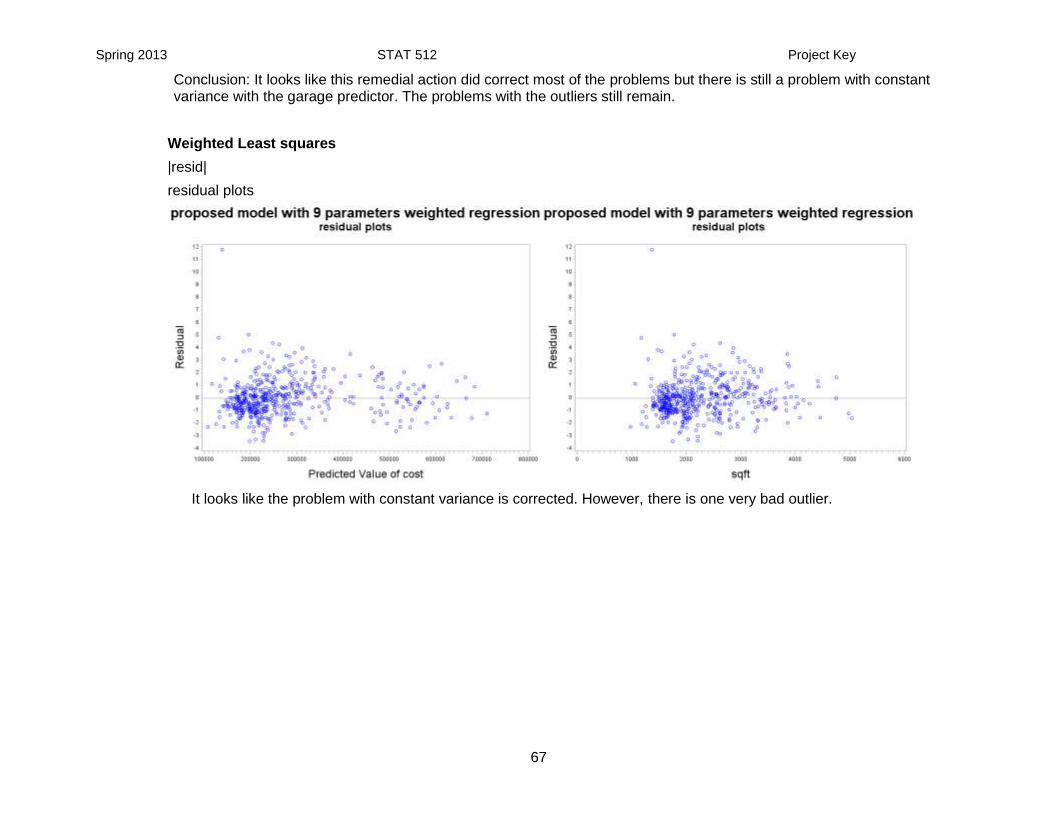
Conclusion: It looks like this remedial action did correct most of the problems but there is still a problem with constant variance with the garage predictor. The problems with the outliers still remain.

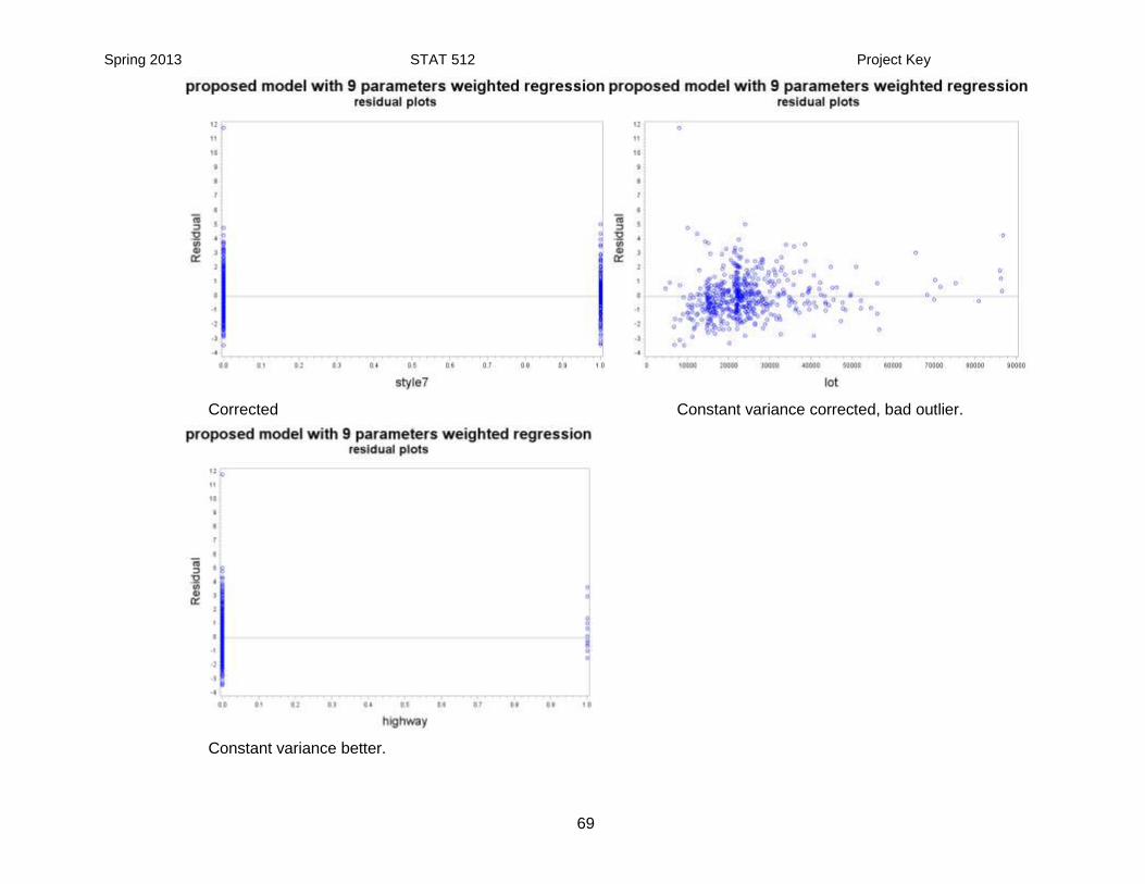
Weighted Least squares

|resid|

residual plots

It looks like the problem with constant variance is corrected. However, there is one very bad outlier.


68

Constance variance: corrected, bad outlier Constant variance better, bad outliers.

Constant variance better, bad outlier Constant variance better.


69

Corrected Constant variance corrected, bad outlier.

Constant variance better.


70

normality plots

Now, the data looks slightly right skewed, but this is due to one outlier.


71

resid2

residual plots

problems have been corrected.

Constant variance seems to be mostly corrected, but there is still a problem with outliers.


72

Constant variance is better, still outliers Constant variance better. No outliers

Constant variance corrected. No outliers Constant variance corrected, still outliers.


73

Constant variance better, still a problem with highway = 1

normality plots

The normality is slightly improved, but still a problem with long tails.


74

Because |resid| plots have a very bad outliers and resid2 plots don’t have this problem, the better weighting system is with resid2.

Ridge Regression

Since this method does not correct a problem with assumptions, no output is required.

(c) Regenerate any of the other parts (a) – (e) in question 6 that are required to be sure that all of the assumptions are met. Again, comments are necessary on all plots. If any assumptions are still not met, what would you do next to correct the problem? Please explain your answer. YOU DO NOT NEED TO PERFORM ANY MORE REMEDIAL ACTIONS!

Y transformations

I am not going to redo the outlier/influential points information because we didn’t perform a full analysis of the points in the first place. The only additional plots required are for the partial regression plots.

sqft: this is definitely significant, it does look linear and the problems with the outliers seems to be less.


garage: this is significant and again there is a problem with the outliers.

year: this is significant and again there is a problem with the outliers. It looks like the curvature has been corrected.

qual1: this is significant and it looks like the problems with the outliers is less than before.


75

style1: this does not look significant

style7: this looks significant and there is a problem with outliers.

lot: this is significant and again there is a problem with the outliers.

highway: this is hard to tell because of the small number of points at 1.

This method makes the assumptions more appropriate.


76

WLS

I am not going to redo the outlier/influential points information because we didn’t perform a full analysis of the points in the first place. The only additional plots required are for the partial regression plots.

|resid|

sqft: this is definitely significant, it does look linear and the problems with the outliers seems to be less.


garage: this seems to make it more bunched up so there is more of a problem with outliers then before.

year: similar to garage, this seem to increase the problem with the outliers.

qual1: this separated this variable into two distinct groups.


77

style1: this does not look significant and made the outliers worse.

style7:this looks significant and increased the problem with outliers.

lot: this is less significant and increased the problem with outliers.

highway: this made this better and more linear though there is still a problem with outliers.

In general, this method made the outliers worse so I would not use this particular weighting scheme.


78

resid2

sqft: this is definitely significant, it looks like there is some curvature now and the variance is larger.

bath: this is significant and it looks like there is a serious problem with the outliers.

garage: this is more spread out but there are still outlier problems.

year: this looks a little more bunched up so it increases the problem with the outliers.

qual1: this separated this variable into two distinct groups.


79

style1: this does not look significant and made the outliers worse.

style7:this looks significant; the problems with the outliers is similar to before

lot: this is more bunched up so the problems with the outliers increases.

highway: improves the situation a little.

This method does help with the assumptions though there are still serious problems.


80

Ridge Regression

Since this method does not correct a problem with assumptions, no output is required.

Further remedial action: There is still a problem with constant variance, so performing a weighted regression with different weighting method or a non-parametric regression might be needed. In addition, the large number of outliers in this data set might be causing both the problem with constant variance and normality. I would look at the outliers/influential points in more detail and see if the points really do look influential. A possible remedial action for this is to rerun the analysis without the outlying points (one at a time) and see if the results change. In addition, robust regression might be performed or another method that is not as influenced by these points.

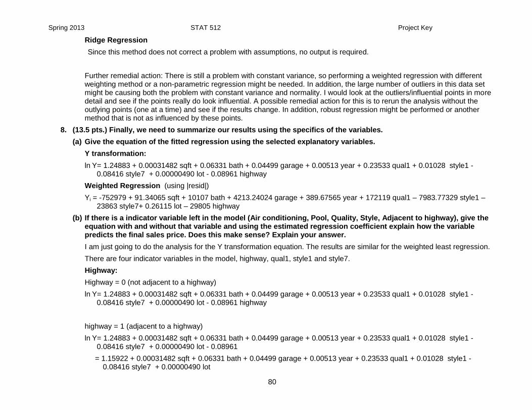
8. (13.5 pts.) Finally, we need to summarize our results using the specifics of the variables.

(a) Give the equation of the fitted regression using the selected explanatory variables.

Y transformation:

ln Y= 1.24883 + 0.00031482 sqft + 0.06331 bath + 0.04499 garage + 0.00513 year + 0.23533 qual1 + 0.01028 style1 - 0.08416 style7 + 0.00000490 lot - 0.08961 highway

Weighted Regression (using |resid|)

Yi = -752979 + 91.34065 sqft + 10107 bath + 4213.24024 garage + 389.67565 year + 172119 qual1 – 7983.77329 style1 – 23863 style7+ 0.26115 lot – 29805 highway

(b) If there is a indicator variable left in the model (Air conditioning, Pool, Quality, Style, Adjacent to highway), give the equation with and without that variable and using the estimated regression coefficient explain how the variable predicts the final sales price. Does this make sense? Explain your answer.

I am just going to do the analysis for the Y transformation equation. The results are similar for the weighted least regression.

There are four indicator variables in the model, highway, qual1, style1 and style7.

Highway:

Highway = 0 (not adjacent to a highway)

ln Y= 1.24883 + 0.00031482 sqft + 0.06331 bath + 0.04499 garage + 0.00513 year + 0.23533 qual1 + 0.01028 style1 - 0.08416 style7 + 0.00000490 lot - 0.08961 highway

highway = 1 (adjacent to a highway)

ln Y= 1.24883 + 0.00031482 sqft + 0.06331 bath + 0.04499 garage + 0.00513 year + 0.23533 qual1 + 0.01028 style1 - 0.08416 style7 + 0.00000490 lot - 0.08961

= 1.15922 + 0.00031482 sqft + 0.06331 bath + 0.04499 garage + 0.00513 year + 0.23533 qual1 + 0.01028 style1 - 0.08416 style7 + 0.00000490 lot


81

Because there are no interaction terms, this has the effect of decreasing the intercept. The coefficient is negative which means being adjacent to the highway decreased the cost. This makes sense because the area around the house is more congested, etc. To me, I want to be close to the main roads, but not on them; again this is personal preference.

Qual1

Qual1 = 0 (low or medium quality)

ln Y= 1.24883 + 0.00031482 sqft + 0.06331 bath + 0.04499 garage + 0.00513 year + 0.01028 style1 - 0.08416 style7 + 0.00000490 lot - 0.08961 highway

qual1 = 1 (high quality)

ln Y= 1.48416 + 0.00031482 sqft + 0.06331 bath + 0.04499 garage + 0.00513 year + 0.01028 style1 - 0.08416 style7 + 0.00000490 lot - 0.08961 highway

Because there are no interaction terms, this has the effect of increasing the intercept. The coefficient is positive which means that if the quality of the house is high the house costs more. This makes sense.

Style1

Style1 = 0 (all styles except 1)

ln Y= 1.24883 + 0.00031482 sqft + 0.06331 bath + 0.04499 garage + 0.00513 year + 0.23533 qual1 - 0.08416 style7 + 0.00000490 lot - 0.08961 highway

style1 = 1 (style 1)

ln Y= 1.25911 + 0.00031482 sqft + 0.06331 bath + 0.04499 garage + 0.00513 year + 0.23533 qual1 - 0.08416 style7 + 0.00000490 lot - 0.08961 highway

This data implies that if the house has style 1, it costs more. Since I don’t know what that style is, I can’t state if it makes sense or not.

Style7

Style7 = 0 (all styles except 7)

ln Y= 1.24883 + 0.00031482 sqft + 0.06331 bath + 0.04499 garage + 0.00513 year + 0.23533 qual1 + 0.01028 style1 + 0.00000490 lot - 0.08961 highway

style7 = 1 (style 7)

ln Y= 1.16467 + 0.00031482 sqft + 0.06331 bath + 0.04499 garage + 0.00513 year + 0.23533 qual1 + 0.01028 style1 + 0.00000490 lot - 0.08961 highway

This data implies that if the house has style 7, it costs less. Again, I can’t state if it makes sense or not.


82

(c) For the continuous variables, explain how each variable predicts the final sales price. Does this make sense? Explain your answer.

sqft: this has a positive slope which makes sense, the larger the square feet, the sales price is higher.

bath: again, this has a positive slope which makes sense, the more bathrooms, the sales price is higher.

garage: this makes sense for the same reason as before.

year: the newer the house, the higher the sales price.

lot: the larger the lot, the higher the sales price.

(d) To me (having recently bought a house), all of the predictor variables are important in the sales price. Can you think of a reason why not all of the predictors are in the final model. (Possible reasons: multicollinearity, all houses have it, very few houses have it, variety of preferences.) There should be one statement per predictor variable NOT in the final model.

number of bedrooms: A reason why this might not be included is because this is related to the number of bathrooms and size of the house. There was a pairwise correlation in this study.

air conditioning: Maybe an equal number of people wanted it or didn’t want it. I did check the data, not all of the houses had air conditioning. However, most of them did include it.

Pool: Again, this might be a non-issue because of different preferences of the buyers. If you don’t want a pool and the house has a pool, it might lower the price. If you want a pool and the house doesn’t have a pool it could lower the price, etc.

quality: A reason why low quality is the only one that is included is that most people cannot determine the difference between medium and high quality when buying a house.

style: Since we don’t know what the individual styles are, it is hard to answer this part. However, this could go back to personal preference. For example, when I bought a house, I wanted a ‘split design’ one story. However, if there are young kids, it might be preferable to not have the split design with more than one story.

(e) Though we are not including any interaction terms in this model, can you think any of the possible interaction terms might have been important in this model? Why or why not? (You just need to include one possibility.) Rerun your chosen model given in part a) including your chosen interaction term (remember that both of the first order terms need to be included if they are not already there). Is this interaction term important? Please comment.

I can think of a couple of obvious interactions that might be relevant in this study.

1) number of bedrooms/number of bathrooms – think about this situation, if there are two bedrooms then there might be little difference between the price of 1 and 2 bathrooms, however, if there are 3 bedrooms, I would expect the price to be much lower for 1 bathroom versus 2 bathrooms.

2) square feet/lot size: I would hope that the lot size is a certain percentage larger than the square feet of the house.

3) pool/square feet/lot size: If there is a pool, the lot size should be even larger.

4) bedrooms/garage: If there are more bedrooms, there might need to be a larger garage.


83

I am sure there are other interaction terms that might have been important in this model. This part is going to be graded on if the reason makes sense.

Results using the Y-transformed data.



Mean Square

F Value Pr > F

Model 11 81.56512 7.41501 243.70 <.0001

Error 510 15.51780 0.03043


Root MSE 0.17443 R-Square 0.8402

Dependent Mean 12.43463 Adj R-Sq 0.8367

Coeff Var 1.40280


84

Parameter Estimates


Standard Error

t Value Pr > |t|

Intercept 1 1.17299 1.08649 1.08 0.2808

sqft 1 0.00032702 0.00002191 14.92 <.0001

bed 1 0.09630 0.01975 4.88 <.0001

bath 1 0.17982 0.02473 7.27 <.0001

garage 1 0.03334 0.01502 2.22 0.0269

year 1 0.00500 0.00055727 8.97 <.0001

qual1 1 0.25353 0.03112 8.15 <.0001

style1 1 0.02323 0.01894 1.23 0.2205

style7 1 -0.07115 0.02420 -2.94 0.0034

lot 1 0.00000503 6.999645E-7 7.19 <.0001

highway 1 -0.10695 0.05404 -1.98 0.0483

bedbath 1 -0.03453 0.00632 -5.46 <.0001

In this model, the interaction term IS important because the interaction term has a P-value of <0.0001. See my explanation above concerning why this is relevant. Remember that even though bed was originally not significant, it still needs to be included in the model because we added the interaction term. Since bed is now significant, this means that this is not an appropriate method of adding interaction terms. The preferred method is to include all of the interaction terms in the original model and then perform the model selection and continue the project from there. I did not use this method in this project because of the complexity of the full model even if you only include pairwise interactions.

Note: To perform this step with the weighted regression, the following steps are required: 1) Generate the new weights using the different model (you may use the same methodology either |resid| or resid2 as before, 2) run the regression.

Instead of adding the interaction term AFTER remedial actions were performed as was stated in the project, this should really be added before the remedial actions were performed in step 7. The following is the output from the model of

Y= 0 + 1 sqft + 2 bed + 3 bath + 4 garage + 5 year + 6 qual1 + 7 style1 + 8 style7 + 8 lot + 9 highway + 10 bed*bath


85



Mean Square

F Value Pr > F

Model 11 8.247384E12 7.497622E11 229.86 <.0001

Error 510 1.663528E12 3261819101


Root MSE 57112 R-Square 0.8322

Dependent Mean 277894 Adj R-Sq 0.8285

Coeff Var 20.55183

Parameter Estimates


Standard Error

t Value Pr > |t|

Intercept 1 -2853418 355734 -8.02 <.0001

sqft 1 105.79513 7.17443 14.75 <.0001

bed 1 9727.78050 6465.37974 1.50 0.1330

bath 1 29338 8095.37168 3.62 0.0003

garage 1 8448.32919 4917.26528 1.72 0.0864

year 1 1405.39805 182.45805 7.70 <.0001

qual1 1 129928 10190 12.75 <.0001

style1 1 18349 6200.29441 2.96 0.0032

style7 1 -24326 7923.78392 -3.07 0.0023

lot 1 1.36095 0.22918 5.94 <.0001

highway 1 -38701 17694 -2.19 0.0292

bedbath 1 -5266.53432 2069.92765 -2.54 0.0112


86

This time the interaction term is still significant (and style1), but bed, garage are not significant. Remember, bed is required to be in the model. Again, you can see that adding additional terms does change which factors are significant. Please keep this in mind when you are doing model selection in your future career. It is a very complicated process to figure out which predictor variables are significant and the answer is not necessarily unique. Therefore, you need to be very careful when you report your conclusions.

spring 2013 stat 512 project key project key part 1 (90 ...lfindsen/stat512/projectkey.pdf ·...

Documents