spring 2002 ©, 2002, m.s. daskin, northwestern u. 1...

Spring 2002 ©, 2002, M.S. Daskin, Northwestern U. 1

Example Use of SITATION

Mark S. Daskin

Department of IE/MS

Northwestern U.

Evanston, IL


Two problems to be solved

1. Minimize the demand weighted total distance (or average distance)• Using 10 facilities

• To serve the 150 largest demands in the continental US

2. Find tradeoff between the % of covered demands and the average distance with• A coverage distance of 300 miles

• And 8 facilities


First step

Double click on the SITATION.EXE software.

This will load the software. You will see an

ABOUT box for about 2-3 seconds followed by

the main menu


Here is the main menu

First you have to load

the dataset you want to

load.

Click on Load Data


To load the data ….

First tell SITATION what

kind of distances you are

using

• Euclidean (straight line)

• Great Circle (shortest distance

on a sphere)

• Manhattan (right angle)

• Network

Click on GREAT CIRCLE


Now

Click on Specify

Demand File


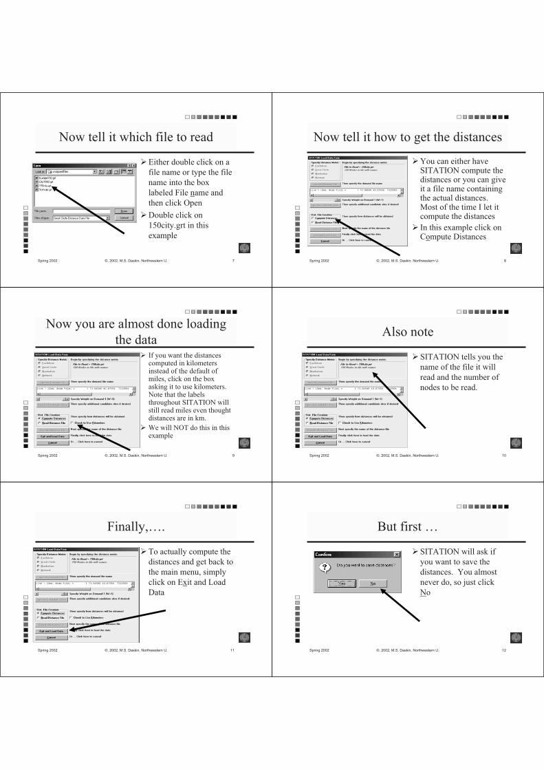
Now tell it which file to read

Either double click on a

file name or type the file

name into the box

labeled File name and

then click Open

Double click on

150city.grt in this

example


Now tell it how to get the distances

You can either have SITATION compute the distances or you can give it a file name containing the actual distances.Most of the time I let it compute the distances

In this example click on Compute Distances


Now you are almost done loading

the dataIf you want the distances computed in kilometers instead of the default of miles, click on the box asking it to use kilometers.Note that the labels throughout SITATION will still read miles even thought distances are in km.

We will NOT do this in this example


Also note

SITATION tells you the

name of the file it will

read and the number of

nodes to be read.


Finally,….

To actually compute the

distances and get back to

the main menu, simply

click on Exit and Load

Data


But first …

SITATION will ask if

you want to save the

distances. You almost

never do, so just click

No


Now you are back at the Main Menu

You must now specify the coverage distance and a cost per mile evenif the model to be run does not call for these values. They are used for reporting purposes

Click on Set Parameters


Now …

Type in a coverage

distance (e.g., 300)

And a cost per mile (e.g.,

1)


Now

If you notice the Done and Run box is now available.Clicking this will allow you to go back to the Main Menu. You can also force sites in or out of the solution using the Force Nodes option. We will not do that in this example.

Click Done and Run


Before getting back to the Main

MenuSITATION tells you

how large the cover list

is. This is just for

information purposes

and you can usually

ignore it.

Click OK


Now

SITATION will let you

run either single or

multiple objective

(Tradeoff Curve)

problems. We want a

single objective problem

(the P-median problem)

so click on Run Models


First you must tell SITATION

which problem to solveClick on the

problem to be

solved. In our

case we want the

P-median

problem


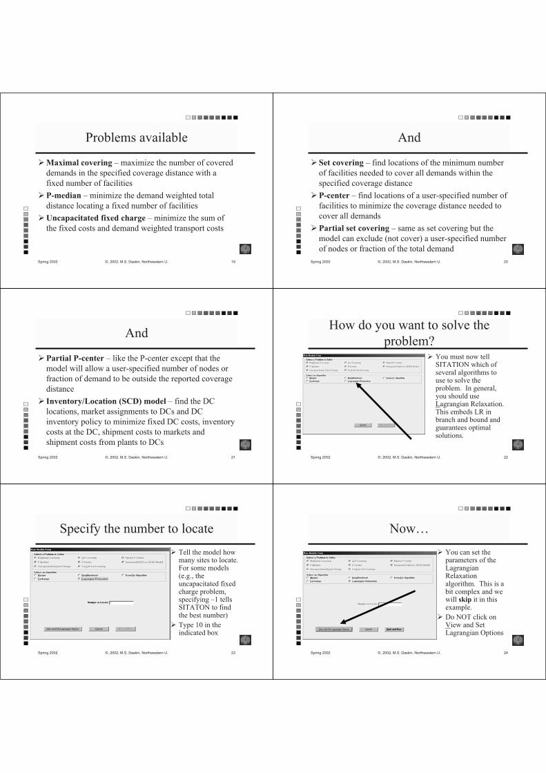
Problems available

Maximal covering – maximize the number of covered

demands in the specified coverage distance with a

fixed number of facilities

P-median – minimize the demand weighted total

distance locating a fixed number of facilities

Uncapacitated fixed charge – minimize the sum of

the fixed costs and demand weighted transport costs


And

Set covering – find locations of the minimum number

of facilities needed to cover all demands within the

specified coverage distance

P-center – find locations of a user-specified number of

facilities to minimize the coverage distance needed to

cover all demands

Partial set covering – same as set covering but the

model can exclude (not cover) a user-specified number

of nodes or fraction of the total demand


And

Partial P-center – like the P-center except that the

model will allow a user-specified number of nodes or

fraction of demand to be outside the reported coverage

distance

Inventory/Location (SCD) model – find the DC

locations, market assignments to DCs and DC

inventory policy to minimize fixed DC costs, inventory

costs at the DC, shipment costs to markets and

shipment costs from plants to DCs


How do you want to solve the

problem?You must now tell SITATION which of several algorithms to use to solve the problem. In general, you should use Lagrangian Relaxation. This embeds LR in branch and bound and guarantees optimal solutions.


Specify the number to locate

Tell the model how many sites to locate.For some models (e.g., the uncapacitated fixed charge problem, specifying –1 tells SITATON to find the best number)

Type 10 in the indicated box


Now…

You can set the parameters of the LagrangianRelaxationalgorithm. This is a bit complex and we will skip it in this example.

Do NOT click on View and Set Lagrangian Options


We are now ready to run the model

By clicking on

Quit and Run

you ask

SITATION to

solve the

problem


Lagrangian Progess Form

This form tells you

information about

the progress of the

algorithm

including the

bounds on the

solution


The total number of iterations


And

Information on

the branch and

bound tree


And …

Which nodes are

forced in (+) out

(-) and

undecided (0) at

this point in the

branch and

bound algorithm


And …

What percent of

the branch and

bound tree has

been explored

so far


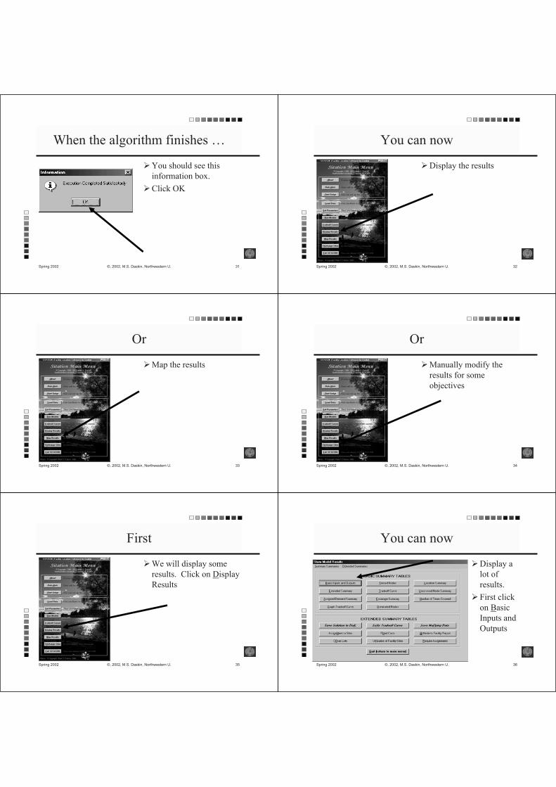
When the algorithm finishes …

You should see this

information box.

Click OK


You can now

Display the results


Or

Map the results


Or

Manually modify the

results for some

objectives


First

We will display some

results. Click on Display

Results


You can now

Display a

lot of

results.

First click

on Basic

Inputs and

Outputs


This summary shows

A summary

of the basic

model inputs


And

Model outputs including the problem and algorithm being solved, statistics on how long it took to solve it, and the objectivefunction values


Go back

Once you

have studied

this report

click Cancel

to return to

the menu of

reports


Now see where you locate

Click on

Extended

Summary to

see where

SITATION

located

facilities


Extended Summary

This tells you where you locate facilities, the number of covered demands, the % of demands covered, the average weighted distance, and the total cost


And the verdict is…

Note that

the

average

weighted

distance

should be

127.13

miles if

you solved

this

correctly


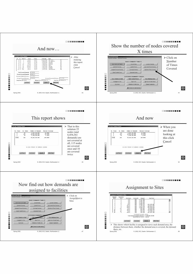
And now…

After

studying

this report

click

Cancel


Show the number of nodes covered

X timesClick on

Number

of Times

Covered


This report shows

That in this solution 25 nodes (and 6,454,361demands) are not covered at all, 115 nodes are covered once and 10 are covered twice


And now

When you

are done

looking at

this click

Cancel


Now find out how demands are

assigned to facilitiesClick on

AssignMent to

Sites


Assignment to Sites

This shows which facility is assigned to serve each demand area, the distance between them, whether the demand area is covered, the demand there, etc.


Assignment to Sites

As well as the maximum assigned distance and the total demand

weighted distance


Go back ….

Click on Cancel to go back to the reports menu


And so on

There are many

other reports,

graphs (for

some

problems) and

options to save

results.

Experiment

with them.

They should be

self

explanatory.


Go back to the Main Menu

To get

back to the

main

menu,

click Quit

(return to

main

menu)


Now we can Map the solution

Click on Map Results


Tell it what the border file is

If you have a file giving

the coordinates of the

border of the region

under study, click Yes;

otherwise click No

Click Yes now


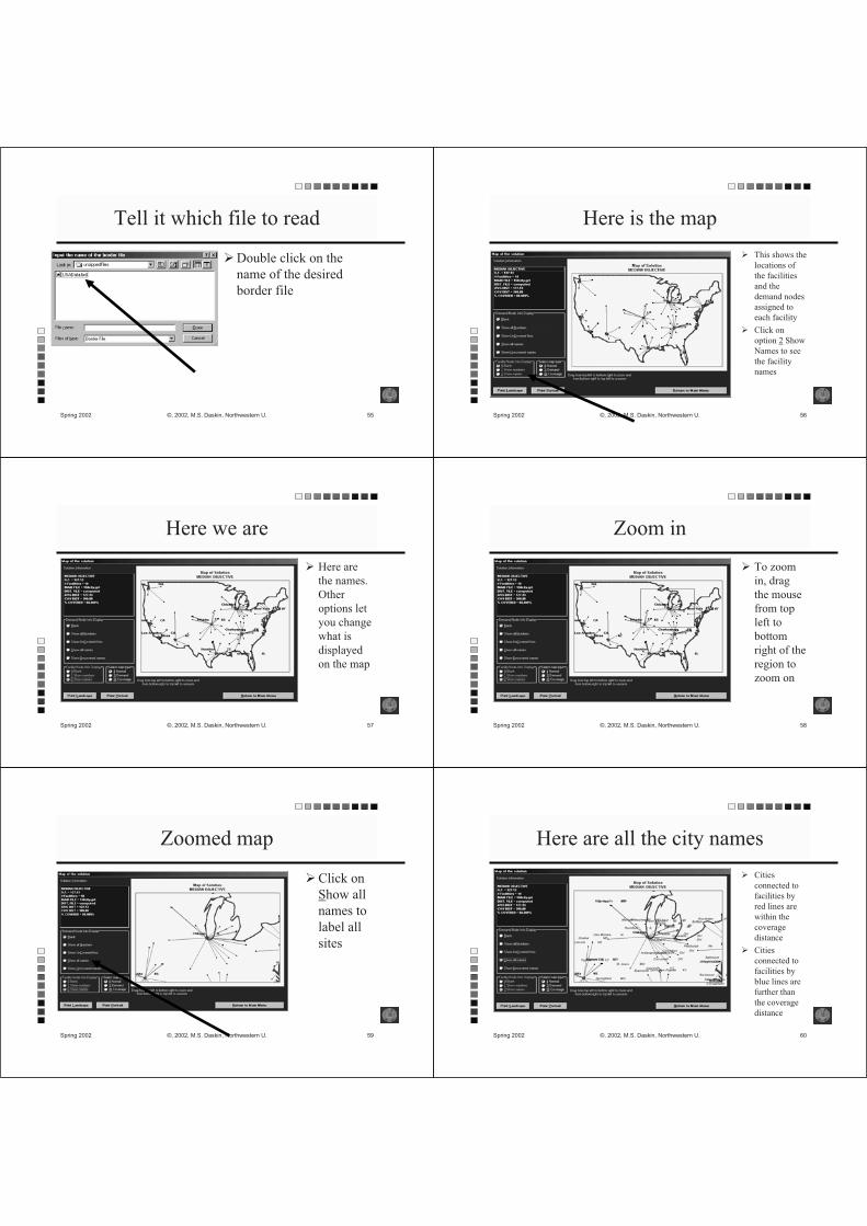
Tell it which file to read

Double click on the

name of the desired

border file


Here is the map

This shows the

locations of

the facilities

and the

demand nodes

assigned to

each facility

Click on

option 2 Show

Names to see

the facility

names


Here we are

Here are

the names.

Other

options let

you change

what is

displayed

on the map


Zoom in

To zoom

in, drag

the mouse

from top

left to

bottom

right of the

region to

zoom on


Zoomed map

Click on

Show all

names to

label all

sites


Here are all the city names

Cities

connected to

facilities by

red lines are

within the

coverage

distance

Cities

connected to

facilities by

blue lines are

further than

the coverage

distance


Zoom out

To return to

the original

map, drag a

box from

the lower

right to the

upper left


Get rid of city names

Click on

Blank to

get rid of

the city

names


Now see other maps

Click on

%

Demand

to see the

relative

demands


Map of relative demands

Note the

high bars

at New

York and

Los

Angeles

Now click

@

Coverage


Coverage map

This map

draws a line

between any

pair of cities

that are

within the

coverage

distance of

each other.


Go back

Click on $

Normal to

see the

map of the

solution

again.


Go back again…

Click on

Return to

Main

Menu to

go back to

the Main

Menu


Now try exchanging sites

Click on Exchange Sites

to manually change the

solution.

Note that this option is

not available with all

objectives.


Exchange sites

In this example, we will see what happens if we locate in Philadelphiainstead of New York

Click Exchange2 Sites


Add Philadelphia

Click on

Philadelphia


Tell SITATION to add it

Click on Pick

node to Add


Tell SITATION which node to

removeHighlight New

York (it should

already be

highlighted)


Tell it to delete New York

Click on Pick

node to Drop


Now

SITATION will show you a message telling you the impact of the change (in this case, among other impacts, the average distance will go up by 6.45 miles)

Tell SITATION whether you want to make the change

Click Yes in this case


Now

Look carefully and there is now a facility in Philadelphia and no facility in New York

Click Close to go back to the Main Menu


You could now

Display the results of

these manual changes or

map the new solution,

etc.

But we will skip all that.

You should now know

how to do all of that.


Instead

We will quickly go

through the tradeoff

curve options

Click on Tradeoff

Curves


SITAION helps you out

To prevent you from

inadvertently losing

solutions, SITATION

asks if you really want to

run a new model

Click Yes


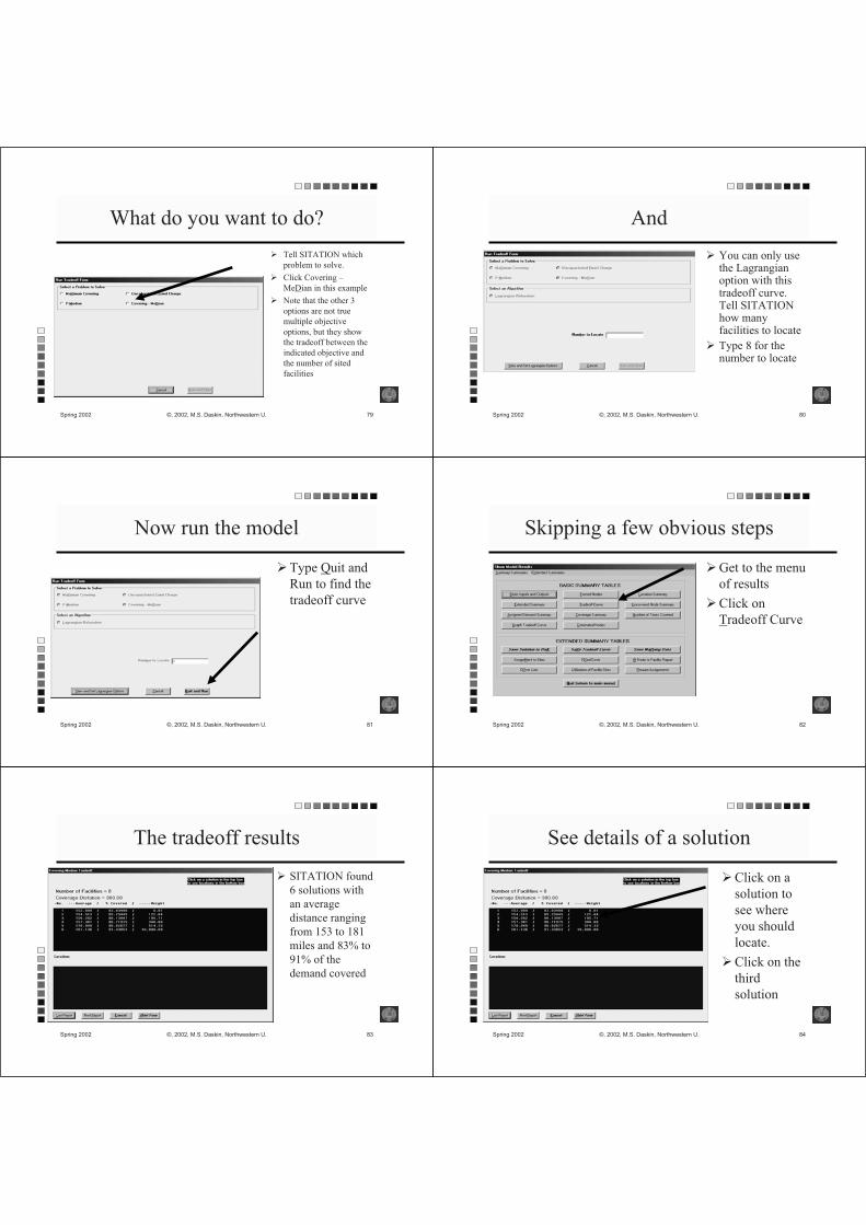
What do you want to do?

Tell SITATION which

problem to solve.

Click Covering –

MeDian in this example

Note that the other 3

options are not true

multiple objective

options, but they show

the tradeoff between the

indicated objective and

the number of sited

facilities


And

You can only use the Lagrangianoption with this tradeoff curve.Tell SITATION how many facilities to locate

Type 8 for the number to locate


Now run the model

Type Quit and

Run to find the

tradeoff curve


Skipping a few obvious steps

Get to the menu

of results

Click on

Tradeoff Curve


The tradeoff results

SITATION found

6 solutions with

an average

distance ranging

from 153 to 181

miles and 83% to

91% of the

demand covered


See details of a solution

Click on a

solution to

see where

you should

locate.

Click on the

third

solution


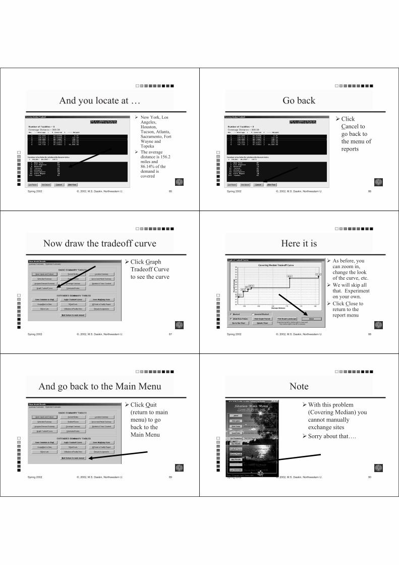
And you locate at …

New York, Los Angeles,Houston,Tucson, Atlanta, Sacramento, Fort Wayne and Topeka

The average distance is 156.2 miles and 86.14% of the demand is covered


Go back

Click

Cancel to

go back to

the menu of

reports


Now draw the tradeoff curve

Click Graph

Tradeoff Curve

to see the curve


Here it is

As before, you can zoom in, change the look of the curve, etc.

We will skip all that. Experiment on your own.

Click Close to return to the report menu


And go back to the Main Menu

Click Quit

(return to main

menu) to go

back to the

Main Menu


Note

With this problem

(Covering Median) you

cannot manually

exchange sites

Sorry about that….


Map the solutions

Click on Map results to

see where you locate for

each solution on the

tradeoff curve


You get a blank map !!!

Click on the

solution

number you

want to see in

the box in the

top left corner

Click on

solution 3

now


Now

And now, as before, ask SITATIONto show the facilitynames

Click on 2ShowNames


Here is the solution

You can click on

other solutions

and the map will

automatically

update itself

Try it and then…

Click Return to

Main Menu


Now we can get out of SITATION

Click Exit SITATION


Again

To prevent you from

inadvertently leaving

before you want to,

SITATION asks you to

confirm that you really

want to exit

Click Yes


And finally

Click OK to return to

Windows


SITATION is (hopefully)

Relatively easy to understand if you know a bit

about location models.

Relatively bullet proof. It should be very hard

to crash it.

Try other options on your own


And note

You can print any of the reports, graphs or maps

just by clicking on the appropriate Print button.


Enjoy

Have fun using SITATION. Experiment with

• Forcing facility sites into or out of the solution

• Other objective functions

• Etc.

spring 2002 ©, 2002, m.s. daskin, northwestern u. 1...

Documents