spousal joint retirement: a reform based approach to ... · pdf filespousal joint retirement:...
TRANSCRIPT
Spousal Joint Retirement:
A Reform Based Approach to Identifying Spillover Effects↑↑↑↑
Francois Gerard and Lena Nekby∗
Abstract
This study uses a recent Swedish pension reform to identify spillover effects of a change in spousal pension incentives on own pension behavior. A difference-in- difference-in-difference identification strategy is used exploiting variation across cohorts treated by national pension reforms as well as variation within cohorts across sectors treated by local public sector pension reforms which enhanced the work incentives of the national pension reform. Results indicate that pension reforms had both a direct effect on retirement behavior due to changes in own pension incentives and an indirect effect via changes in spousal retirement incentives. A conservative estimate suggests that ignoring the impact of spousal spillover effects underestimates the impact of the pension reform by as much as 14 percent.
↑ Financial support from The Institute for Labor Market Policy Evaluation (IFAU Project number 2010:126) is gratefully acknowledged. The authors are grateful for comments from Gabriella Sjögren Lindqvist as well as seminar participants at the Uppsala Center for Labor Studies Mini-workshop on Family Economics, the Institute for Labor Market Policy Evaluation (IFAU), the Department of Economics at Linnaeus University and Umeå University and the Swedish Institute for Social Research (SOFI). ∗ Gerard: Department of Economics, UC Berkeley, e-mail: [email protected]. Nekby: Department of Economics, Stockholm University and Institute for Future Studies, e-mail: [email protected]
1. Introduction
Due to aging populations and severe imbalances in pension systems, recent pension reforms in
the US and Europe aim to increase retirement ages by strengthening work incentives for the
elderly. How current and future reforms will affect the labor supply of the elderly is thus a
central question of interest for policymakers. It is, however, a complicated issue as evidence
suggests that retirement decisions, at least within couples, are highly interdependent. Coile
(2003) estimates that neglecting the influence of spousal retirement incentives on own retirement
behavior may underestimate the overall impact of a typical reform by 13% to 20%. Although
many studies analyze the determinants of joint retirement, the literature to date has not been able
to clearly identify the impact of a partner’s retirement decision on own pension behavior. In this
study, spill-over effects of a change in spousal pension incentives on own pension behavior is
analyzed exploiting a recent Swedish pension reform to identify effects of interest.
2. Previous Literature
Evidence of interdependent retirement decisions comes from three strands in the literature. First,
many studies indicate that joint retirement is a common phenomenon, accounting for nearly a
third of retirement patterns in the US and Europe (Blau, 1998; Coile, 2003; Hurd, 1990; Maestas,
2002; Pozzoli and Ranzani, 2009). Blau (1998), using the Retirement History Survey estimates
that between 11% -16% of couples exit the labor force in the same quarter and between 30%-
41% within one year of each other. Hurd (1990) finds similar proportions using the New
Beneficiary Survey. The issue of potential spill-over effects has also become more salient over
time as an increasing number of elderly wives are in the work force. Pozzoli and Ranzani (2009)
estimate that 78% of working males in Europe are married and 24% have working wives.
Participation rates of elderly females are even higher in the Scandinavian countries where 65%
of females aged 50-64 are in the labor force.
Second, numerous empirical studies estimate significant and economically relevant
correlations between individual retirement decisions and partner incentives (An et al, 1999;
Coile, 2003; Johnson and Favreault, 2001; Zweimuller et al., 1996).1 Coile (2003), for example,
finds that men are very responsive to their wives’ pension incentives but women less responsive
to their husbands' incentives. Zweimuller et al. (1996) finds a similar asymmetric correlation
where husbands react to changes in wives’ legal minimum retirement age but wives don’t react
vice versa. An et al. (1999) finds strong complementarities in leisure between spouses in
Denmark, but symmetrically for husband and wife. Pozzoli & Ranzani (2009) find asymmetries
in terms of how spousal health correlates with retirement decisions. Wives in European countries
are more likely to take care of their sick partners, and retire earlier, whereas husbands do not.
Johnson and Favreault (2001) instead find for the US, that both men and women are less likely to
retire if spouses have left the labor market for health reasons.2 Kapur and Rogowski (2007) find
that access to employer-provided health insurance is associated with increased joint retirement
probabilities among dual-earner couples.
These studies, however, lack a clear identification strategy for estimating spillover
effects. Recent work exploits exogenous changes from pension reforms to estimate causally the
impact of own retirement incentives on own retirement behavior (Glans 2008; Mastrobuoni,
2009). Glans (2008) uses the same pension reform in Sweden used in this study, a reform that
increased work incentives differentially across birth cohorts. Based on duration models, Glans
1 Note that all of the empirical studies listed here rely entirely on survey data characterized by small sample sizes, especially when restricted to couples. 2 See also Kapur and Rogowski (2007) who study if access to employer-provided health insurance increases joint retirement probabilities
finds a decline in retirement hazards among cohorts most affected by the reform indicating a
delay in retirement behavior. Results were especially noticeable among public sector workers
affected by both national and local public sector pension reforms. Mastrobuoni (2009) uses a
change in the national retirement age in 2000 to estimate the effect of Social Security incentives
on labor supply. Results indicate an increase in the mean retirement age of affected cohorts by
about half as much as the increase in the national retirement age. Our work extends this approach
to spillovers within couples.
Very few papers have studied the interdependence of retirement decisions with a clear
research design. Baker (2002) studies the retirement behavior of married couples using the
introduction of the Spousal Allowance in Canada, a targeted support for women in poor families.
Results show that the allowance is associated with a decline in labor force participation among
male spouses in eligible couples. However, benefits were means-tested (at the household level)
implying almost mechanically, a strong negative effect on husbands’ labor supply. Stancanelli
(2012) exploits retirement age legislation in France as well as a policy reform requiring younger
cohorts born after 1933 to pay longer pension contribution periods to identify spousal spillover
effects on work hours. The work hours of both spouses are found to fall significantly upon own
and partner’s retirement.3
Given difficult identification issues, the third strand in the literature instead estimates
structural models of retirement behavior within couples (Hurd, 1990; Gustman and Steinmeier,
2000; Maestas, 2002). These studies find that correlation in tastes for leisure as well as
complementarities in the value of leisure between spouses go a long way in explaining why
3 More recently, Brown and Laschever (2012) estimate peer effects in retirement decisions in the context of the workplace rather than within couples. See also numerous papers studying the interdependence of labor supply decisions within couples in other contexts such as income taxation (Gelber, 2012), unemployment benefits (Cullen and Gruber, 2000) and sick leave (Olson and Skogman Thoursie, 2010).
spouses coordinate retirement decisions (Gustman and Steinmeier, 2000). Maestas (2002) adds
bargaining power to a retirement model and shows that the impact of complementarities in
leisure on joint retirement is enhanced when wives have greater decision-making power within
couples.
Recently, Selin (2011) studies spousal spillover effects on retirement behavior using the
same reform studied here.4 Selin studies male reactions to changes in the retirement incentives
among female spouses only. His identification strategy is to analyze the retirement behavior of
men married to women aged 63 from 2000-2005, i.e. comparing the retirement behavior of men
who have 63 year old wives in 2000 and who therefore are born in 1937, the last cohort
unaffected by national and local public sector pension reforms, with men who have spouses aged
63 in each of the years from 2001 to 2005 (who therefore belong to cohorts affected by the
pension reforms). Although Selin uses the same variation across spousal cohorts and sector of
employment that we use, Selin only has one reference year, wives aged 63 in the year 2000. In
addition, he departs from a generous definition of retirement (any pension income) which
implies, as husbands are on average two years older than female spouses, that the vast majority
of husbands are defined as retired. In other words, results are driven by a smaller subset of
husbands who are closer in age or younger than their female spouses. Finally, it is unclear to
what degree Selin accounts for the direct effect of pension reforms on own pension behavior
among husbands in the analysis.
Our study follows the labor supply decisions of both married men and women belonging
to cohorts born from 1930 to 1950. We are able to observe and follow these cohorts from 1985 to
2006. As such we have information on numerous cohorts unaffected by the reform (1930-1937)
4 Our project was granted financial support by the Institute for Labor Market Policy Evaluation (IFAU) in October 2010. Selin’s working paper was published in July 2011.
as well as those affected by the reform (1938-1950). In addition, as the reform was implemented
in the year 2001 and our data extends back to 1985, our data permits a better analysis of pre-
treatment trends in retirement behavior and fewer problems with left censoring. Finally, our
identification strategy accounts for both the direct (change in own retirement incentives) and
indirect (change in spousal retirement incentives) reform effects on individual retirement
behavior.
The rest of the paper is set up as follows. Section 3 provides a description of the Swedish
pension reform while Section 4 provides a short theoretical overview of the mechanisms behind
joint retirement. Data and the identification strategy are described in Section 5 and results
reported in Section 6. Concluding remarks are found in Section 7.
3. The Swedish Pension System- Now and Before
3.1 The Swedish Pension Reform (2001)
Discussions about the need to reform the Swedish pension system commenced in the 1980s. Like
many European countries, an ageing population together with a generous public pension system
implied large projected deficits in the pension system. In 1992, a parliamentary working group
with wide political representation published a report outlining the forthcoming pension reform,
the details of which were worked out in the ensuing years. Final legislation concerning the new
pension system, which went from a defined benefit system to a defined contribution system, was
passed in June 1998. In 2001, the first pension payments were made within the new pension
system marking the implementation of the new pension system, which was fully up and running
at the end of the following year.5 Specifically, it is from 2001 that early withdrawals from the
new system could be made for cohorts affected by the pension reform (those born 1938 or later).
5 See Sundén (2006) and Sjögren Lindqvist and Wadensjö (2006) for overviews of the Swedish pension reform.

The pension reform introduced a national defined contribution system in comparison to
the old defined benefit system (described below). The new system consists of three parts, an
income pension (notional defined contribution), a premium pension and a guarantee pension.
Over and beyond are occupation-based pensions (determined by collective agreements) and
private pensions. Contributions to income pensions in the new system are recorded in individual
accounts, the value of which represents claims to future pensions. Annual contributions are
however used to finance current pension benefit obligations as in a pay-as-you-go system, hence
accounts are notional.
Income and premium pensions are based on lifetime earnings including pensionable
income from sickness benefits, parental leave, unemployment insurance, military service and
studies (if financed by national student loans). A proportion, 18.5 percent of pensionable income,
is assigned annually to an individual pension account of which 16 percentage points are credited
to notional individual income pension and 2.5 percentage points to the fully funded premium
pension account.6 Premium pensions are individually invested into at most five funds registered
by the Premium Pension Authority (PPM).7 Guarantee pensions are paid to those with low or
zero income pensions, are means tested according to earned income and premium pensions, and
are financed outside the national pension system via general tax revenues.
6 The insured pays seven percent through a national pension contribution up to a ceiling of 8.07 Basic Income Amounts (the Basic Income Amount (BIA) was SEK 37,700 in 2001 and SEK 48,000 in 2008). Employers pay 10.21 percent of wages to the pension system regardless of income level, but only contributions up to the ceiling are assigned to the individual pension account. This 17.21 percent corresponds to 18.5 percent of the pension base. The discrepancy is due to the fact that the national pension contribution of seven percent is deducted from income when the pension base is calculated (0.93*8.07BIA=7.5BIA). The pension base has a ceiling of 7.5 BIA (before taxes) per year. 7 Benefits from premium pensions can be shared between spouses or registered partners. In the event of a transfer between spouses, the amount is reduced by 14 percent as most transfers are expected to go from husbands with higher incomes to wives with longer expected lifetimes.
Pensions can be withdrawn at the earliest from age 61, with a reduction until age 65, and
there is no upper age limit for beginning pension withdrawals.8 Pension payments are adjusted
for economic growth and the lifetime expectancy of the birth cohort to which an individual
belongs. Higher life expectancy leads to lower income pensions and economic growth leads to
higher pensions through indexation. In comparison to the old defined benefit system, the new
system provides incentives for postponed retirement due to a closer link between lifetime income
and pension benefits. In addition, the automatic adjustment of benefits due to changes in life
expectancy implies that individuals in later cohorts must postpone retirement in order to gain the
same replacement rate as those belonging to earlier cohorts (Sundén, 2006).
3.2 The Old Pension System
In brief, the old pension system consisted of two parts a flat guaranteed pension (folkpension)
introduced in 1913 and a supplementary benefit (allmänn tillägspension, ATP) introduced in
1960.9 The flat guaranteed pension was independent of previous income while the supplementary
benefit was calculated as 60 percent of the Price Basic Amount (PBA) times the average ATP
points earned during the 15 highest years of income since age 16.10 ATP points were, in turn,
calculated annually as pensionable income in excess of PBA divided by the PBA.11
ATP = 0.60 * PBA* ATP points
8 The mandatory retirement age within the four main collective agreements was set to age 67 in 1991. However, this rule was negotiable until 2001 and all four of the main collective bargaining areas set the mandatory retirement age to 65. A legislative change in 2001 set the mandatory retirement age to 67. However, as current agreements were honored, the legal mandatory retirement age for the vast majority of workers changed from 65 to 67 first on January 1 2003. 9 The folkpension was initially more of a defined contribution system and means-tested. Over time, a number of reforms pushed the system towards a defined benefit system and eased means-testing. The pension reform of 1948 made pensions independent of pension contributions as well as income and wealth and increased pension levels (Sjögren Lindqvist and Wadensjö, 2006). 10 The Price Basic Amount (PBA) is calculated based on changes in the general price level, in accordance with the National Insurance Act (2010:110). Calculations are based on the change in the Consumer Price Index and established for the entire calendar year. The PBA was 36,900 SEK in the year 2001 and 41,000 SEK in 2008. 11 For those with less than 15 (but more than three) years income, ATP points were calculated as the average over the available years. In order to earn full ATP pensions, individuals must have worked 30 years. For those with less than 30 years, ATP pensions were reduced by a factor calculated as the number of years worked divided by 30.
ATP points = (pensionable income – PBA)/PBA
Pensions could be withdrawn from the beginning of the month an individual turned 61 with a
permanent reduction of 0.5 percent for each month left until age 65.12 Pension withdrawal could
also be postponed until the month an individual turned 70 with a permanent increase of 0.7
percent for each postponed month. Unlike the new system, work after age 70 did not lead to
higher pensions in the old system.13
3.3 Transition to the New Pension System
Transition to the new pension system will occur gradually over a period of 16 years. The first
cohort to participate in the new system is the 1938 cohort. For this cohort, one-fifth of pensions
are from the new system and four fifth from the old system (see Table 1 for a graphical
depiction). Each cohort thereafter increases its participation in the new system by 1/20 implying
that those born in 1954 or later participate fully in the new system. The last cohort unaffected by
the pension reform is therefore the 1937 cohort. It is this variation across cohorts that will be
used to identify the direct and indirect effects of the reform on individual retirement behavior as
well as variation in pension incentives across sectors of employment due to reforms of
occupational pensions, described below.14
12 The lower age limit changed twice. When ATP was introduced in 1960, the lower age limit for pension withdrawals was set to age 63. In 1976, the formal retirement age was reduced from 67 to 65 and the lower age limit reduced to age 60. In January 1998, the lower age limit was increased to age 61 in order to conform to the lower age limit of the new pension system. 13 Note that there was a close link between retirement pensions and disability pensions in the old system. Indeed, from 1970, disability pensions for those 63 and older could be granted for both medical and labor market reasons and from 1972, elderly unemployed without unemployment benefits were entitled to disability pensions based solely on labor market reasons. Disability pensions in the old system were often used as a pathway to early retirement (Palme and Svensson, 1999, 2002). Disability pensions were reformed together with the national pension reform of 2001. 14 Note that there is a guarantee clause in the new pension system for cohorts affected by the reform (1938-1953) guaranteeing that pensions under the new system will not be lower than the supplementary pension earned in the old system up to the year 1994.
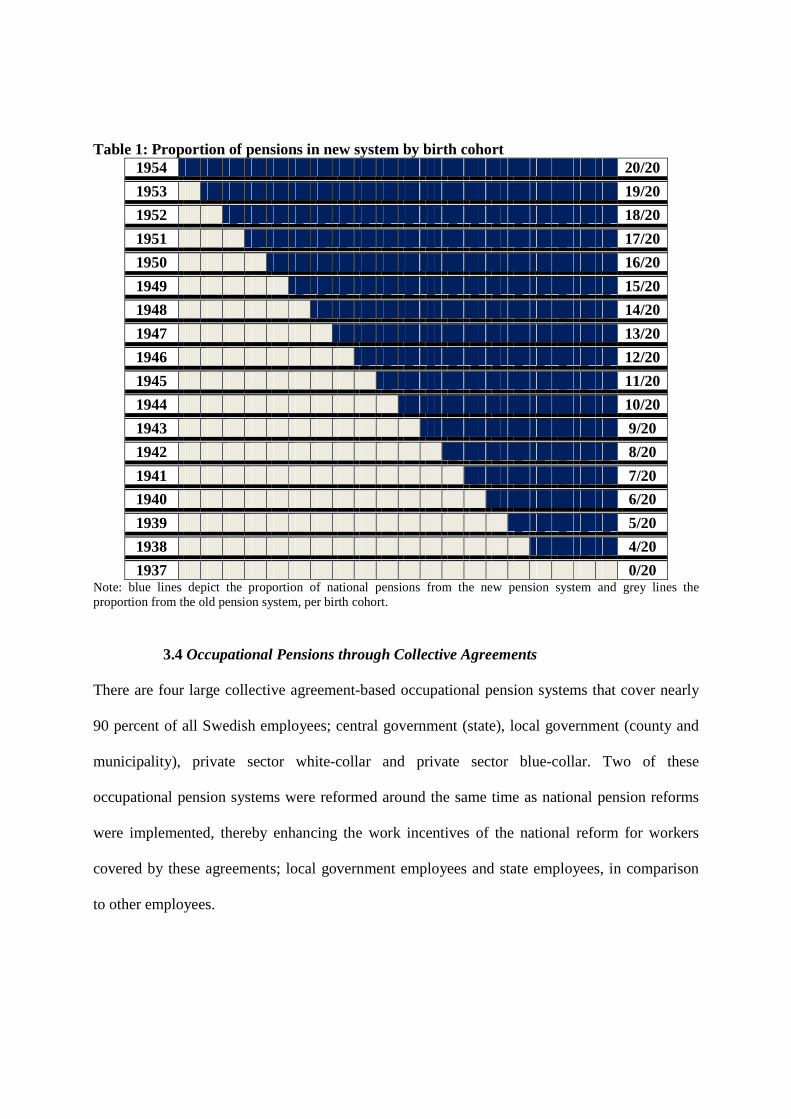
Table 1: Proportion of pensions in new system by birth cohort 1954 20/20
1953 19/20
1952 18/20
1951 17/20
1950 16/20
1949 15/20
1948 14/20
1947 13/20
1946 12/20
1945 11/20
1944 10/20
1943 9/20
1942 8/20
1941 7/20
1940 6/20
1939 5/20
1938 4/20
1937 0/20 Note: blue lines depict the proportion of national pensions from the new pension system and grey lines the proportion from the old pension system, per birth cohort.
3.4 Occupational Pensions through Collective Agreements
There are four large collective agreement-based occupational pension systems that cover nearly
90 percent of all Swedish employees; central government (state), local government (county and
municipality), private sector white-collar and private sector blue-collar. Two of these
occupational pension systems were reformed around the same time as national pension reforms
were implemented, thereby enhancing the work incentives of the national reform for workers
covered by these agreements; local government employees and state employees, in comparison
to other employees.
Two new agreements (PFA-98 and PFA-01) together reformed occupational pensions for
employees in the local public sector (municipal and county employees). Similar to the national
pension reform, cohorts born in 1937 or earlier were unaffected by local public sector pension
reforms. The new local public sector pension system consists of two parts, a defined contribution
and a supplementary defined benefit for incomes above 7.5 increased PBA. This in comparison
to the old system (PA-KL) which was based on a defined benefit system where the average of
the five highest income years, during the seven years prior to retirement, was used to calculate
pension benefits. In the new system, the size of pensions depends on annual income and the size
of pension contributions.15 Employers pay a premium of 3.5 percent of individual annual income
up to 7.5 percent of PBA. Contributions are paid into individual accounts which workers can
place in traditional insurance or pension funds.16 Employer contributions increased, with PFA-
01, to 4 - 4.5 percent of individual annual income (up to 7.5 PBA), depending on date and sector
of employment (municipal/county).17 Pensions from the individual defined contribution part of
occupational pensions can be withdrawn from the age of 55. The duration of pension payments is
chosen individually either for a limited period of at least five years or lifelong.18 The new local
public sector pension system came into effect on January 1, 2000 for those born in 1938 or
later.19
15 Initially, annual pension contributions were made from the age of 28 (revised in 2002 to age 21 for all local government workers except those with white-collar positions). 16 Originally there was a minimum limit of 40 percent of full-time employment for pension contributions. No limit was introduced in 2002. Before 2003, not everyone could decide fully over the placement of their individual pension contributions. However, at least one percent was controlled individually. As of 2003, all individuals can decide how to invest the full defined contribution part of pension contributions. 17 A new agreement in 2006 brings employer contributions to similar levels for all local public sector workers. 18 Supplementary pensions for local public sector workers are paid to those who have pensionable incomes exceeding 7.5 (increased) PBA. This portion of pensions is a benefit based system calculated as a percentage of average annual incomes exceeding 7.5 PBA. 19 See also Selin (2011) for a detailed description of the local public sector occupational pension reform.
For central government workers (State) employees a new pension system was
implemented for those born in 1943 or later effective from January 1, 2003. The new system
(PA-03) consists of two defined contribution pensions (individual and supplementary) and a
defined benefit portion for those whose pension basis exceeds 7.5 PBA per year. Employer
contributions in the new system are equal to 2.3 percent of pensionable annual income in the
individual pension and 1.9 percent in the supplementary pension. Individual pensions could be
earned from the age of 23 and benefits are paid for life from the age of 65. Supplementary
pensions are usually paid for five years from the age of 65.
In short, the new national pension system, which reformed the pension system from a
defined benefit to a defined contribution system, was implemented in 2001 when the first
pension payments under the new system were made. Municipal and county workers have a
similar change in the occupational pension system, implemented in in 2000, enhancing the work
incentives of the national pension reform for local public sector workers vis-à-vis workers under
other collective agreements.20 In 2001, the year the national pension reform was implemented,
the first cohort of local public sectors affected by the reform, the 1938 cohort, turned 63.
Variation in pension incentives created by the staggered implementation across cohorts in the
national system as well as variation across occupational pensions within cohorts will be used to
identify spillover effects of a change in spousal retirement incentives on own retirement
behavior.
4 Theoretical overview
Several theoretical mechanisms suggest an interdependence of retirement decisions within
couples. The income and retirement benefits of the spouse affect the wealth level of the 20 Private sector blue-collar workers switched to a defined contribution system from a supplementary defined benefit system already in 1996 whereas private sector white-collar workers reformed their defined benefit system towards a defined contribution system first in 2007.
household, given joint resources, as well as the demand for leisure (Lazear, 1986). In general, a
positive change in the annuity rate of retirement benefits implies higher income as well as an
increase in the price of leaving the labor force. Higher income has a negative income effect on
labor supply implying earlier retirement while the higher price of leisure leads to a substitution
effect and delayed retirement, regardless if the source is a change in own or spousal
income/pension benefits, given that family resources are pooled. It has been argued that for men
the substitution effect dominates so that an increase in retirement benefits leads to delayed
retirement while for women, due to greater responsibilities for home production, the income
effect may dominate.
A preference for shared leisure between spouses may induce a higher probability of own
retirement following or adjacent to spousal retirement regardless if this is due to
complementarities in leisure or selection, i.e., assortative mating of individuals with similar
preferences for leisure. Higher joint wealth or other joint assets would then increase joint
retirement probabilities. Spouses may also have similar pension incentives due to similarities in
age, sector of work and/or joint pension saving and may partially coordinate retirement decisions
due to better information of the retirement system due to spillover effects in knowledge between
couples.
There are also potential cross-health effects among elderly couples where one spouse
may retire early to care for an ailing partner or, rather, postpone retirement to cover increased
medical expenses. As noted in the overview by Lunsdaine and Mitchell (1999), longer life
expectancy and earlier retirement suggest that many retirement age individuals are likely to face
caregiving responsibilities in conjunction with retirement decisions and that a disproportionate
amount of this responsibility is likely to fall on women. Elderly women, aged 55-64, are more
likely to transition from work and caregiving responsibilities to caregiving only (Lunsdaine and
Mitchell, 1999). On the other hand, some studies find that working women may delay retirement
when their spouse is in poor health (Pozzebon and Mitchell, 1989; Johnson and Favreault, 2001).
Several models emphasize that decisions concerning joint retirement are the result of
bargaining between spouses. As such, the relative decision making power of each spouse in a
household bargaining framework may push spouses towards or against joint retirement (Maestas
2002). Structural models attempting to fit models to the data appear to primarily disagree on the
source of heterogeneity between couples and on the adequate modeling of the household
decision-making process. While being aware of these mechanisms, we take a step back and
concentrate on the causal estimation of a change in spousal retirement incentives on own
retirement behavior.
5 Data and Empirical Setup
5.1 Data
Data comes from the IFAU Database which has gathered information from numerous registers
available at Statistics Sweden. In this study, employment information from the Labour Statistics
Based on Administrative Sources (RAMS) available from 1985-2000 is combined with income
and employment information from the Longitudinal Database about Income, Education and
Employment (LOUISE) available from 1990-2008. Information on employment, sector, income
and education is therefore available from 1985 while information on various sources of pension
income from both the new and old system is available from 1990.21 The dataset covers the entire
population residing in Sweden between the ages of 16-65 for the years 1985-2000 and for the
population aged 16-74 for the years 2001-2008. Due to family identification numbers, married
21 From 1990, information on income stemming from early retirement, the flat guaranteed pension and supplementary pension from the old system as well as income pension, premium pension and guarantee pensions in the new system are available as is information on private pensions and occupational pensions (at an aggregate level).
spouses or cohabitants registered as living in the same household with children in common can
be matched to each other.22
We restrict the analysis to the years prior to 2007, as several sectors reform occupational
pensions thereafter. We focus on couples who have the same spouse (or cohabitating partner)
throughout the observation period and on cohorts born from 1930 to 1950. Missing are couples
where one spouse falls outside the registered age range, dies during the observation period or
where no match was found between the LOUISE and RAMS datasets. The majority, 54 percent,
of the circa 1.3 million individuals observed in the original data (1985-2008) are with the same
spouse throughout the observation period. Approximately 24 percent were constantly single and
18 percent changed spouses. The remaining four percent are individuals who appear to be
married based on marital/family status but who are not matched to a spouse through a family
identification number.
As it is unclear how to define the exact date of retirement, four definitions are tested in
the analysis, all based on (registered) measures of work or pension income (real income in 2008
prices):23
1. Permanent drop in income – A permanent drop in annual work income (including sick
benefits) of at least 33 percent from one year to the next.
2. No work – Annual work income equal to zero.
3. Some pension – The sum of all annual pension income sources greater than zero.
22 Data on couples stem from household information. To date, Statistics Sweden tracks only married couples, couples in same-sex registered partnerships and cohabitants with common children. 23 Three common definitions of retirement are otherwise used in the literature; (1) receiving retirement pension regardless of current employment status, (2) being out of the labor force regardless of the reason for being out of work and receipt of pension income and (3 )self-declaration (in surveys) of pension status regardless of employment status and receipt of pension income.
4. More pension – The sum of annual work income plus sick benefits is less than the sum
of all annual pension income.
Two of these retirement definitions, a permanent “drop in income” and “no work”, are based on
information available from 1985 onwards while the other definitions are based on pension
information available first in 1990. Focus in the analysis as well as in the presentation of results
is on the first retirement definition as it is based on data available from 1985 and is a less strict
definition of retirement than the “no work” definition. The sensitivity of results to other
measures, however, will also be tested. In the analysis, those coded as retired in the first year
observed, given the definition of retirement used, are dropped from estimation.
As no data is currently available on the collective bargaining area an individual belongs
to in terms of occupational pensions, information on sector of employment is used in the analysis
as a proxy for type of occupational pension.24 An individual’s primary sector of employment
(state, county, municipality or private) is defined as the sector within which an individual earned
the maximum amount of work income before the age of 60.25
Descriptive statistics presented in Table 1 show that there is variation in retirement rates
across the four definitions of retirement. The strictest measure is the “no work” definition while
the most lenient measure is the “some pension” definition. Retirement rates, for the 1937 cohort
in the year 2000, show that females have lower retirement rates on average than their spouses
which is expected due to average age differences between spouses (Column 1). Likewise for
men in the 1937 cohort, men have higher retirement rates than their, on average, younger wives
24 Information on the total annual pension benefits from occupational pensions is available from 1990 but not disaggregated at the sector level. 25 An alternative definition departing from the sector of employment most commonly observed in the annual data before the age of 60 was also tested. Results are not sensitive to choice of definition.
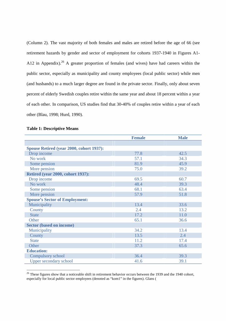
(Column 2). The vast majority of both females and males are retired before the age of 66 (see
retirement hazards by gender and sector of employment for cohorts 1937-1940 in Figures A1-
A12 in Appendix).26 A greater proportion of females (and wives) have had careers within the
public sector, especially as municipality and county employees (local public sector) while men
(and husbands) to a much larger degree are found in the private sector. Finally, only about seven
percent of elderly Swedish couples retire within the same year and about 18 percent within a year
of each other. In comparison, US studies find that 30-40% of couples retire within a year of each
other (Blau, 1998; Hurd, 1990).
Table 1: Descriptive Means
26 These figures show that a noticeable shift in retirement behavior occurs between the 1939 and the 1940 cohort, especially for local public sector employees (denoted as “kom1” in the figures). Glans (
Female Male Spouse Retired (year 2000, cohort 1937): Drop income 77.8 42.5 No work 57.1 34.3 Some pension 81.9 45.9 More pension 75.0 39.2 Retired (year 2000, cohort 1937): Drop income 69.5 60.7 No work 48.4 39.3 Some pension 68.1 63.4 More pension 57.9 51.8 Spouse’s Sector of Employment: Municipality 13.4 33.6 County 2.4 13.2 State 17.2 11.0 Other 65.1 36.6 Sector (based on income) Municipality 34.2 13.4 County 13.5 2.4 State 11.2 17.4 Other 37.3 65.6 Education: Compulsory school 36.4 39.3 Upper secondary school 41.6 39.1
Note: Seven levels of education are used in estimation, disaggregating both compulsory school and upper secondary school to two levels indicting shorter and longer durations within respective level.
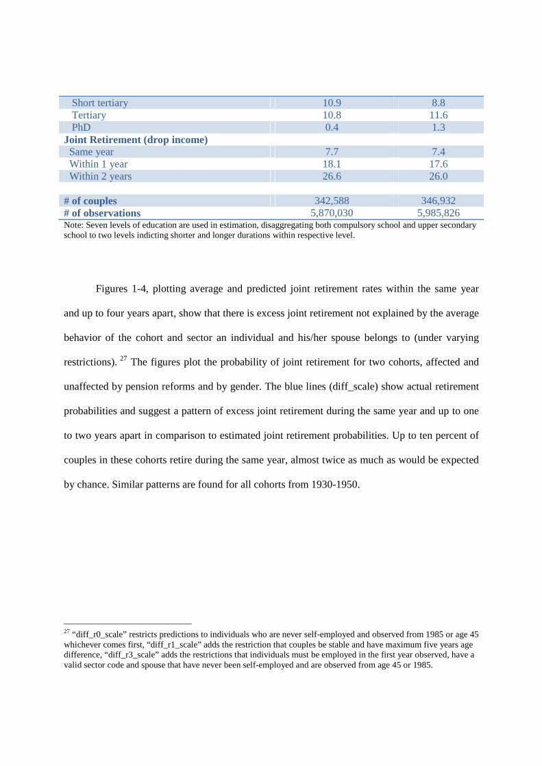
Figures 1-4, plotting average and predicted joint retirement rates within the same year
and up to four years apart, show that there is excess joint retirement not explained by the average
behavior of the cohort and sector an individual and his/her spouse belongs to (under varying
restrictions). 27 The figures plot the probability of joint retirement for two cohorts, affected and
unaffected by pension reforms and by gender. The blue lines (diff_scale) show actual retirement
probabilities and suggest a pattern of excess joint retirement during the same year and up to one
to two years apart in comparison to estimated joint retirement probabilities. Up to ten percent of
couples in these cohorts retire during the same year, almost twice as much as would be expected
by chance. Similar patterns are found for all cohorts from 1930-1950.
27 “diff_r0_scale” restricts predictions to individuals who are never self-employed and observed from 1985 or age 45 whichever comes first, “diff_r1_scale” adds the restriction that couples be stable and have maximum five years age difference, “diff_r3_scale” adds the restrictions that individuals must be employed in the first year observed, have a valid sector code and spouse that have never been self-employed and are observed from age 45 or 1985.
Short tertiary 10.9 8.8 Tertiary 10.8 11.6 PhD 0.4 1.3 Joint Retirement (drop income) Same year 7.7 7.4 Within 1 year 18.1 17.6 Within 2 years 26.6 26.0 # of couples 342,588 346,932 # of observations 5,870,030 5,985,826
Figure 1-4: Actual and Estimated Joint Retirement Probabilities X Years Apart (Individual-Spouse)
5.2 Empirical Setup
Initially the direct effect of the reform is estimated, that is to say the effect of a change in own
pension incentives on own retirement behavior ignoring the potential impact of spousal spillover
effects. This is done in order to compare the size of direct effects with indirect effects generated
through changes in spousal retirement incentives and to compare our causal estimates of the
direct effect with those of previous studies analyzing this question. Our identification strategy
uses the cross-group (cohorts affected/not affected by the reform), cross-time (pre- and post-
reform) and cross-sector (public/private) variation in a difference-in-difference-in-difference
(DDD) setup estimating variations of the following linear probability model:
����(��� = �) = � + ������� + �� +�� + � + ��� (1)
.04
.06
.08
.1.1
2
-4 -2 0 2 4diff_year
diff_scale diff_r0_scalediff_r1_scale diff_r3_scale
Probability of retirement x years apart Women 1935
.04
.06
.08
.1
-4 -2 0 2 4diff_year
diff_scale diff_r0_scalediff_r1_scale diff_r3_scale
Probability of retirement x years apart Women 1940
.04
.06
.08
.1
-4 -2 0 2 4diff_year
diff_scale diff_r0_scalediff_r1_scale diff_r3_scale
Probability of retirement x years apart Men 1935
.04
.05
.06
.07
.08
.09
-4 -2 0 2 4diff_year
diff_scale diff_r0_scalediff_r1_scale diff_r3_scale
Probability of retirement x years apart Men 1940
where yit is a binary variable equal to one if an individual i belonging to group g (g=1 if an
individual belongs to a cohort treated by the national reform) and sector s (s=1 if an individual
belongs to a sector treated by public sector pension reforms) is retired in time t. Reformgst is a
binary variable equal to one for cohorts affected by the national reform g and the public sector
reform s in time t. The model is flexible as it controls for all time-varying group effects, time-
varying sector effects and group-specific sector effects. The benefit of using the DDD model is
that we can control for unobserved factors across cohorts that may be correlated with the
implementation of pension reforms as we ultimately use the variation within cohorts across
sectors over time (assuming that the national reform does not affect the propensity to work in a
certain sector). The model will be estimated with and without a vector of control variables for
individual characteristics such as level of education, industry branch and county of residence.
Thereafter, the indirect effect of a change in spousal retirement incentives on own
retirement is estimated controlling for the direct effect of pension reforms (local and national) on
own retirement behavior using variations of the model:
����(��� = �) = � + ������_� + ������� + ��� (2)
Reform_s is a binary variable equal to one if an individual has a spouse affected by the national
reform g and public sector reforms s in time t. The model includes controls for all individual and
spousal time-varying group effects, time-varying sector effects and group-specific sector effects.
Estimation of spousal spillover effects is based on all individuals including those directly
affected by the reform but controlling for the direct reform effects on individual retirement
probabilities. An alternative strategy would be to drop those directly affected by the reform.
However, this would imply that the variation necessary to identify spousal spillover effects is
severely curtailed, especially for females who tend to be younger than their spouses. The
majority of spouses to females born on or before 1937 who are unaffected by national or local
public sector pension reforms, are born even earlier and also not affected by pension reforms. In
addition, the majority of spouses have less than five years age difference implying that even for
men; a large number of observations are lost for treated spouses if estimation is restricted to
individuals born on or before 1937. Various checks of robustness are of course administered to
determine the sensitivity of results to the inclusion of individuals directly affected by pension
reforms in estimation of spousal spillover effects.
6 Results
6.1 Direct Reform Effect – Changes in Retirement Behavior due to Changes in
Own Retirement Incentives
Results from linear probability estimation of the DDD equation estimating the average reform
effect on own retirement probabilities (based on the drop in income definition of retirement),
using cross-group (cohorts affected/not affected by pension reforms), cross-time and cross-sector
variation, are shown in Table 2. Results indicate a negative treatment effect suggesting that
public sector workers belonging to cohorts affected by both national and occupational pension
reforms delayed retirement to a larger degree than other workers after the reform was
implemented, by approximately 11-12 percentage points.28 Breaking down treatment effects by
year (Columns 2 and 4) indicates that there is an upward trend in retirement behavior, relative to
the reference year 1985, from 1986 to 1997, after which retirement probabilities for those treated
by national and public sector pension reforms begin to decline relative to the control group.29
Treated cohorts appear to have a shift in behavior, in comparison to the control group, prior to 28 When estimation is restricted to fewer cohorts, treatment effects reported here are very similar to those reported in Glans (2008) who uses a similar identification strategy to estimate the direct reform effects on own retirement behavior using cohorts born between 1933-1943. 29 Results are not sensitive to the inclusion of control for education, industry branch and county of residence.
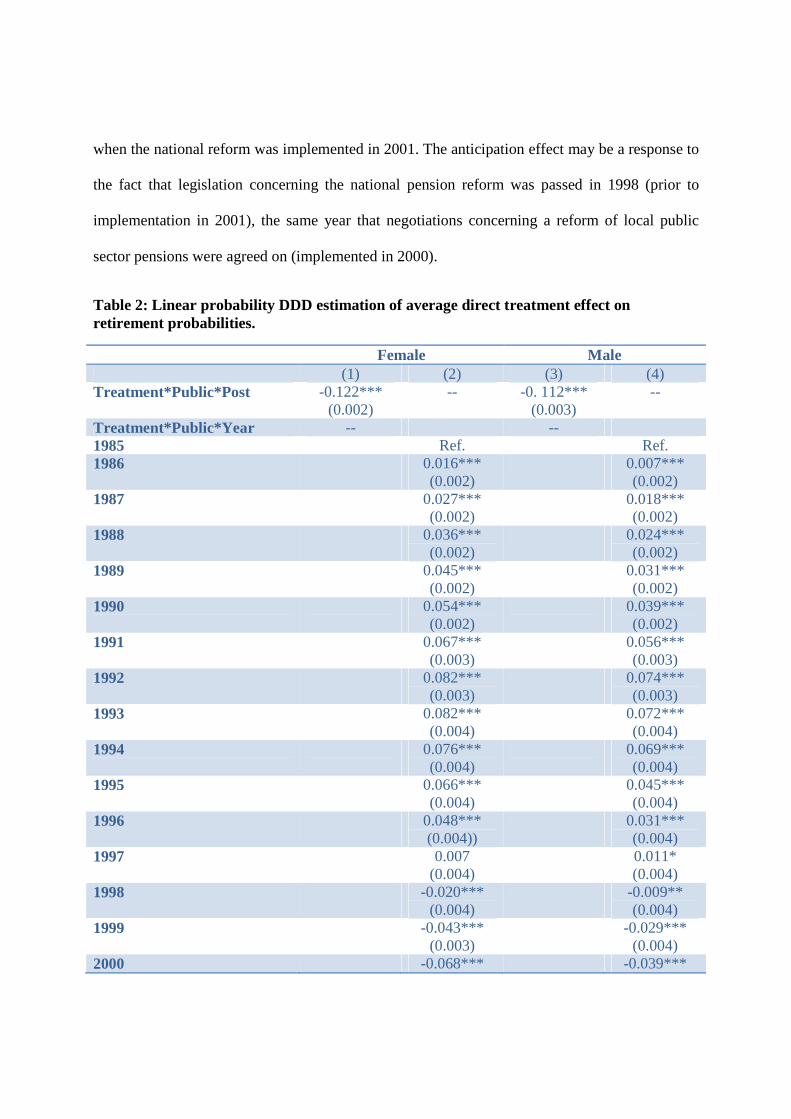
when the national reform was implemented in 2001. The anticipation effect may be a response to
the fact that legislation concerning the national pension reform was passed in 1998 (prior to
implementation in 2001), the same year that negotiations concerning a reform of local public
sector pensions were agreed on (implemented in 2000).
Table 2: Linear probability DDD estimation of average direct treatment effect on retirement probabilities.
Female Male (1) (2) (3) (4) Treatment*Public*Post -0.122***
(0.002) -- -0. 112***
(0.003) --
Treatment*Public*Year -- -- 1985 Ref. Ref. 1986 0.016***
(0.002) 0.007***
(0.002) 1987 0.027***
(0.002) 0.018***
(0.002) 1988 0.036***
(0.002) 0.024***
(0.002) 1989 0.045***
(0.002) 0.031***
(0.002) 1990 0.054***
(0.002) 0.039***
(0.002) 1991 0.067***
(0.003) 0.056***
(0.003) 1992 0.082***
(0.003) 0.074***
(0.003) 1993 0.082***
(0.004) 0.072***
(0.004) 1994 0.076***
(0.004) 0.069***
(0.004) 1995 0.066***
(0.004) 0.045***
(0.004) 1996 0.048***
(0.004)) 0.031***
(0.004) 1997 0.007
(0.004) 0.011*
(0.004) 1998 -0.020***
(0.004) -0.009**
(0.004) 1999 -0.043***
(0.003) -0.029***
(0.004) 2000 -0.068*** -0.039***
(0.003) (0.004) 2001 -0.090***
(0.003) -0.057***
(0.003) 2002 -0.087***
(0.002) -0.076***
(0.003) 2003 -0.127***
(0.002) -0.134***
(0.003) 2004 -0.130***
(0.002) -0.141***
(0.003) 2005 -0.126***
(0.002) -0.137***
(0.003) 2006 -0.123***
(0.002) -0.130***
(0.003) R2 0.28 0.39 0.31 0.45 Observations 5,870,030 5,985,826 Note: Retirement is defined according to the drop in income definition. Treatment is defined as cohorts affected by national reform (cohorts>1937), Public denotes local public sector workers and Post indicates the years after national and public sector pension reforms were implemented (years>2000). Standard errors are clustered at the individual level. Estimations control for education (7 levels), industry branch (two digit branch codes) and county of residence as well as for time-varying treatment effects, time-varying sector effects and sector-specific treatment effects. *** denotes significance at the one percent level, ** at the five percent level and * at the ten percent level.
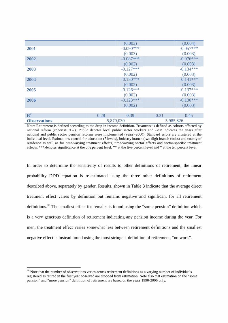
In order to determine the sensitivity of results to other definitions of retirement, the linear
probability DDD equation is re-estimated using the three other definitions of retirement
described above, separately by gender. Results, shown in Table 3 indicate that the average direct
treatment effect varies by definition but remains negative and significant for all retirement
definitions.30 The smallest effect for females is found using the “some pension” definition which
is a very generous definition of retirement indicating any pension income during the year. For
men, the treatment effect varies somewhat less between retirement definitions and the smallest
negative effect is instead found using the most stringent definition of retirement, “no work”.
30 Note that the number of observations varies across retirement definitions as a varying number of individuals registered as retired in the first year observed are dropped from estimation. Note also that estimation on the “some pension” and “more pension” definition of retirement are based on the years 1990-2006 only.
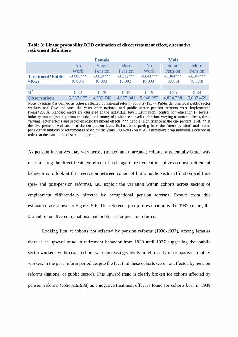
Table 3: Linear probability DDD estimation of direct treatment effect, alternative retirement definitions
Female Male No
Work Some
Pension More
Pension No
Work Some
Pension More
Pension Treatment*Public *Post
-0.086*** (0.003)
-0.024*** (0.003)
-0.112*** (0.002)
-0.041*** (0.003)
-0.064*** (0.003)
-0.107*** (0.003)
R2 0.32 0.28 0.35 0.29 0.35 0.38 Observations 5,787,075 4,769,748 4,967,041 5,948,082 4,824,728 5,037,459 Note: Treatment is defined as cohorts affected by national reform (cohorts>1937), Public denotes local public sector workers and Post indicates the years after national and public sector pension reforms were implemented (years>2000). Standard errors are clustered at the individual level. Estimations control for education (7 levels), industry branch (two digit branch codes) and county of residence as well as for time-varying treatment effects, time-varying sector effects and sector-specific treatment effects. *** denotes significance at the one percent level, ** at the five percent level and * at the ten percent level. Estimation departing from the “more pension” and “some pension” definitions of retirement is based on the years 1990-2006 only. All estimations drop individuals defined as retired at the start of the observation period.
As pension incentives may vary across (treated and untreated) cohorts, a potentially better way
of estimating the direct treatment effect of a change in retirement incentives on own retirement
behavior is to look at the interaction between cohort of birth, public sector affiliation and time
(pre- and post-pension reforms), i.e., exploit the variation within cohorts across sectors of
employment differentially affected by occupational pension reforms. Results from this
estimation are shown in Figures 5-6. The reference group in estimation is the 1937 cohort, the
last cohort unaffected by national and public sector pension reforms.
Looking first at cohorts not affected by pension reforms (1930-1937), among females
there is an upward trend in retirement behavior from 1933 until 1937 suggesting that public
sector workers, within each cohort, were increasingly likely to retire early in comparison to other
workers in the post-reform period despite the fact that these cohorts were not affected by pension
reforms (national or public sector). This upward trend is clearly broken for cohorts affected by
pension reforms (cohorts≥1938) as a negative treatment effect is found for cohorts born in 1938
or later. Public sector workers within each treated cohort are less likely to retire early than other
workers, in comparison to the 1937 cohort from 1938 onwards. The largest negative treatment
effect is found for the 1942 cohort, after which there is a slight upwards trend for later cohorts.
Note that state workers born in 1943 or later are coded as belonging to the treatment group from
2003 due to a pension reform within this sector at this time towards a direct contribution system.
For males, the cohorts unaffected by pension reforms (1930-1937) show no treatment
effects relative to the 1937 cohort implying no differences in pension probabilities between
public sector workers and other workers before and after pension reforms were implemented. As
such, the parallel trends assumption is to a larger degree upheld among elderly males than
females. Similar to females, there is a clear negative treatment affect for cohorts affected by the
reform indicating lower retirement probabilities for public sector workers than other workers
once public sector and national pension reforms came into effect. Notice also that among males,
there is a sharp trend break for the 1943 cohort when state employees are re-coded as belonging
to the treatment group (from 2003 onwards). This break is clearly due to selection effects, i.e.,
male state employees have different pension behavior than other male public sector workers.31
Descriptive statistics in Table 1 show that females are, to a much larger degree, municipal and
county employees in comparison to men and, to a much lower degree, state employees.
Nonetheless, there is a clear negative treatment effect for cohorts born after 1943 in comparison
to the reference group, an effect which gets increasingly negative for later born cohorts.
31 See Figure A13 in Appendix for results of the DDD estimation of a change in own pension incentives on own retirement probabilities where male State employees born after 1942 are not re-coded as belonging to the public sector after 2003. This figure shows clearly that the break for the 1943 cohort is due to selection effects due to a re-coding of public sector affiliation.
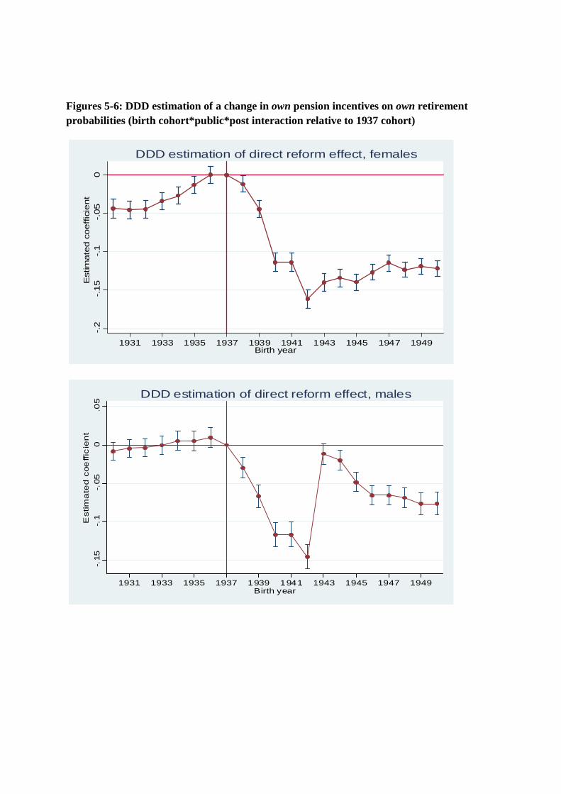
Figures 5-6: DDD estimation of a change in own pension incentives on own retirement probabilities (birth cohort*public*post interaction relative to 1937 cohort)
-.2
-.15
-.1
-.05
0E
stim
ate
d c
oeffic
ient
1931 1933 1935 1937 1939 1941 1943 1945 1947 1949Birth year
DDD estimation of direct reform effect, females
-.15
-.1
-.05
0.0
5
Estim
ate
d c
oe
ffic
ien
t
1931 1933 1935 1937 1939 1941 1943 1945 1947 1949Birth year
DDD estimation of direct reform effect, males
6.2 Indirect Reform Effect (Spousal Spillover Effects) – Changes in Retirement Behavior due to Changes in Spousal Retirement Incentives
Linear probability DDD estimation of a change in spousal incentives on own retirement
behavior, i.e., the average effect of having a spouse belonging to cohorts affected by pension
reforms before and after the reform is implemented, are shown in Table 4. Note that the direct
effect of pension reforms on own retirement is controlled for in estimation. Results indicate
significant and negative treatment effects on retirement probabilities due to changes in spousal
retirement incentives, over and beyond the direct effect due to changes in own retirement
incentives. Having a spouse affected by national and public sector pension reforms reduces
retirement probabilities post-reform, in comparison to those with spouses unaffected by reforms,
by 5-6 percentage points. Coefficient estimates of the direct treatment effect are largely
unaffected in estimation on spousal spillover effects (see Columns 1 and 3). Note also that
estimates of both the direct and indirect reform effect are significant despite considerably more
stringent clustering of standard errors on cohort (own and spouses) and sector (own and spouses)
yielding 1,710 clusters for females and 1,705 clusters for males.
Breaking down the indirect reform effect by year shows, similar to above, that there are
anticipation effects prior to the formal implementation of spousal pension reforms in 2000-2001
for affected cohorts and sectors (Columns 2 and 4). For both females and males, having a spouse
treated by public sector and national pension reforms affects retirement probabilities negatively
and significantly from 1997 (in comparison to the reference year 1985). Prior to 1997,
differences in retirement between those with treated and untreated spouses are positive or
insignificant. The strength of the negative spillover effect increases over time after 1997 in
comparison to the reference year.
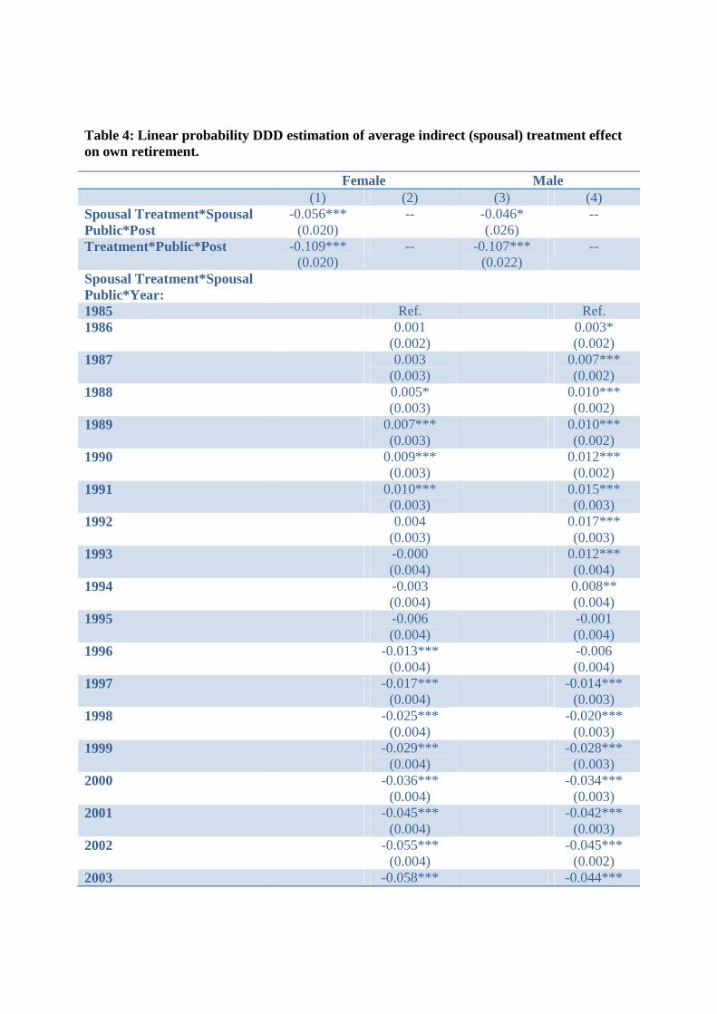
Table 4: Linear probability DDD estimation of average indirect (spousal) treatment effect on own retirement.
Female Male (1) (2) (3) (4) Spousal Treatment*Spousal Public*Post
-0.056*** (0.020)
-- -0.046* (.026)
--
Treatment*Public*Post -0.109*** (0.020)
-- -0.107*** (0.022)
--
Spousal Treatment*Spousal Public*Year:
1985 Ref. Ref. 1986 0.001
(0.002) 0.003*
(0.002) 1987 0.003
(0.003) 0.007***
(0.002) 1988 0.005*
(0.003) 0.010***
(0.002) 1989 0.007***
(0.003) 0.010***
(0.002) 1990 0.009***
(0.003) 0.012***
(0.002) 1991 0.010***
(0.003) 0.015***
(0.003) 1992 0.004
(0.003) 0.017***
(0.003) 1993 -0.000
(0.004) 0.012***
(0.004) 1994 -0.003
(0.004) 0.008**
(0.004) 1995 -0.006
(0.004) -0.001
(0.004) 1996 -0.013***
(0.004) -0.006
(0.004) 1997 -0.017***
(0.004) -0.014***
(0.003) 1998 -0.025***
(0.004) -0.020***
(0.003) 1999 -0.029***
(0.004) -0.028***
(0.003) 2000 -0.036***
(0.004) -0.034***
(0.003) 2001 -0.045***
(0.004) -0.042***
(0.003) 2002 -0.055***
(0.004) -0.045***
(0.002) 2003 -0.058*** -0.044***
(0.004) (0.002) 2004 -0.068***
(0.004) -0.050***
(0.002) 2005 -0.077***
(0.004) -0.050***
(0.003) 2006 -0.084***
(0.004) -0.051***
(0.003) R2 0.27 0.41 0.32 0.46 Observations 5,870,030 5,985,826 Note: Retirement is defined according to the drop in income definition. Treatment (Spousal Treatment) is defined as cohorts (spousal cohorts) affected by national reform (cohorts>1937), Public (Spousal Public) denotes local public sector workers (spousal local public sector worker) and Post indicates the years after national and public sector pension reforms were implemented (years>2000). Standard errors are clustered by cohort, spousal cohort, public sector and spousal public sector affiliation. Estimations control for education (7 levels), industry branch (two digit branch codes) and county of residence as well as for time-varying treatment effects, time-varying sector effects and sector-specific treatment effects. *** denotes significance at the one percent level, ** at the five percent level and * at the ten percent level.
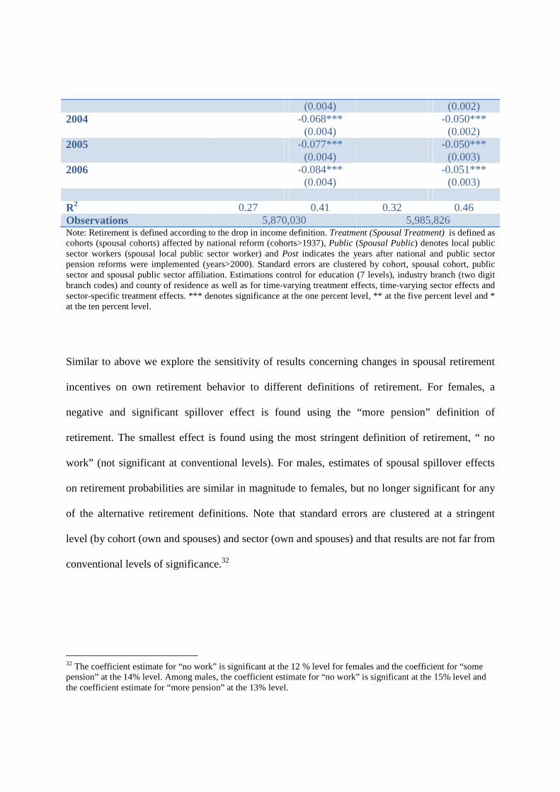
Similar to above we explore the sensitivity of results concerning changes in spousal retirement
incentives on own retirement behavior to different definitions of retirement. For females, a
negative and significant spillover effect is found using the “more pension” definition of
retirement. The smallest effect is found using the most stringent definition of retirement, “ no
work” (not significant at conventional levels). For males, estimates of spousal spillover effects
on retirement probabilities are similar in magnitude to females, but no longer significant for any
of the alternative retirement definitions. Note that standard errors are clustered at a stringent
level (by cohort (own and spouses) and sector (own and spouses) and that results are not far from
conventional levels of significance.32
32 The coefficient estimate for “no work” is significant at the 12 % level for females and the coefficient for “some pension” at the 14% level. Among males, the coefficient estimate for “no work” is significant at the 15% level and the coefficient estimate for “more pension” at the 13% level.
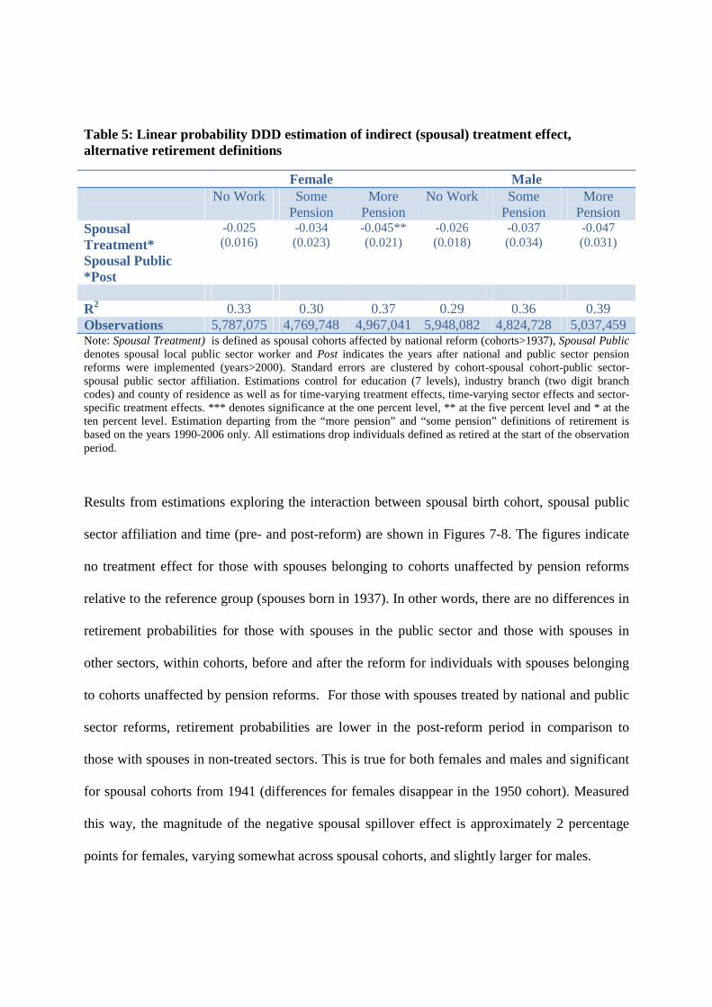
Table 5: Linear probability DDD estimation of indir ect (spousal) treatment effect, alternative retirement definitions
Female Male No Work Some
Pension More
Pension No Work Some
Pension More
Pension Spousal Treatment* Spousal Public *Post
-0.025 (0.016)
-0.034 (0.023)
-0.045** (0.021)
-0.026 (0.018)
-0.037 (0.034)
-0.047 (0.031)
R2 0.33 0.30 0.37 0.29 0.36 0.39 Observations 5,787,075 4,769,748 4,967,041 5,948,082 4,824,728 5,037,459 Note: Spousal Treatment) is defined as spousal cohorts affected by national reform (cohorts>1937), Spousal Public denotes spousal local public sector worker and Post indicates the years after national and public sector pension reforms were implemented (years>2000). Standard errors are clustered by cohort-spousal cohort-public sector-spousal public sector affiliation. Estimations control for education (7 levels), industry branch (two digit branch codes) and county of residence as well as for time-varying treatment effects, time-varying sector effects and sector-specific treatment effects. *** denotes significance at the one percent level, ** at the five percent level and * at the ten percent level. Estimation departing from the “more pension” and “some pension” definitions of retirement is based on the years 1990-2006 only. All estimations drop individuals defined as retired at the start of the observation period.
Results from estimations exploring the interaction between spousal birth cohort, spousal public
sector affiliation and time (pre- and post-reform) are shown in Figures 7-8. The figures indicate
no treatment effect for those with spouses belonging to cohorts unaffected by pension reforms
relative to the reference group (spouses born in 1937). In other words, there are no differences in
retirement probabilities for those with spouses in the public sector and those with spouses in
other sectors, within cohorts, before and after the reform for individuals with spouses belonging
to cohorts unaffected by pension reforms. For those with spouses treated by national and public
sector reforms, retirement probabilities are lower in the post-reform period in comparison to
those with spouses in non-treated sectors. This is true for both females and males and significant
for spousal cohorts from 1941 (differences for females disappear in the 1950 cohort). Measured
this way, the magnitude of the negative spousal spillover effect is approximately 2 percentage
points for females, varying somewhat across spousal cohorts, and slightly larger for males.
Two main results are presented in this section. One, we find a direct reform effect on
individual retirement probabilities implying that workers treated by public sector and national
pension reforms reduced retirement probabilities relative to other workers after the reform was
implemented. The preferred DDD setup showing the interaction between cohort of birth, public
sector affiliation and time (pre- and post-reform) implies that any unobservable differences
between cohorts should be taken into account as variation across sectors of employment within
each cohorts is exploited to identify behavioral effects. Two, we find a significant and negative
indirect reform effect via a change in spousal retirement incentives enhancing the direct effect of
retirement reforms. Spousal spillover effects are found to be large and significant, a result which
is at odds with those reported in Selin (2011). Selin, however, restricts his analysis to males with
63 year old spouses born from 1937-1942 who are observed from 2000-2005. Our results, based
on spousal cohorts born from 1930-1950 observed from 1985-2006; clearly show that spousal
spillover effects become significant for spousal cohorts born first in 1941 or thereafter.33
33 Selin (2011) also departs from the more generous definition of retirement, “some pension” income. Our results using the “some pension” definition continue to show the existence of spousal spillover effects for males but are not either significant at conventional levels (standard errors clustered by cohort-spousal cohort-public sector-spousal public sector affiliation).
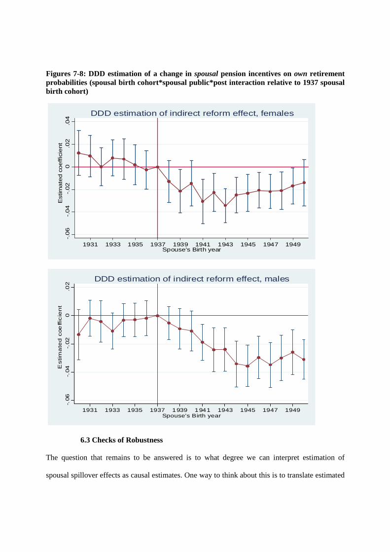
Figures 7-8: DDD estimation of a change in spousal pension incentives on own retirement probabilities (spousal birth cohort*spousal public*post interaction relative to 1937 spousal birth cohort)
6.3 Checks of Robustness
The question that remains to be answered is to what degree we can interpret estimation of
spousal spillover effects as causal estimates. One way to think about this is to translate estimated
-.06
-.04
-.02
0.0
2.0
4E
stim
ate
d c
oeffic
ient
1931 1933 1935 1937 1939 1941 1943 1945 1947 1949Spouse's Birth year
DDD estimation of indirect reform effect, females
-.06
-.04
-.02
0.0
2
Estim
ate
d c
oe
ffic
ien
t
1931 1933 1935 1937 1939 1941 1943 1945 1947 1949Spouse's Birth year
DDD estimation of indirect reform effect, males
effects to an instrumental variable setting, measuring the impact of spousal retirement on own
retirement using the pension reform as an instrument for spousal retirement. Naturally, a pre-
requisite for using an instrument to identify the causal effect of spousal retirement on own
retirement is that the instrument should have no direct effect on individual retirement
probabilities. In the estimation presented above, this is clearly not the case, rather the direct
effect of pension reforms on own retirement behavior is controlled for in estimation of spousal
spillover effects. In order to isolate spousal spillover effects on own retirement free from
potential biases due to direct reform effects, DDD retirement equations are re-estimated for
cohorts not directly affected by national and public sector pension reforms, i.e., cohorts born on
or before 1937 and/or non-public sector employees. Note that as females are married to spouses
that are on average two years older, potential spousal reform effects for females are driven by
those with younger spouses.
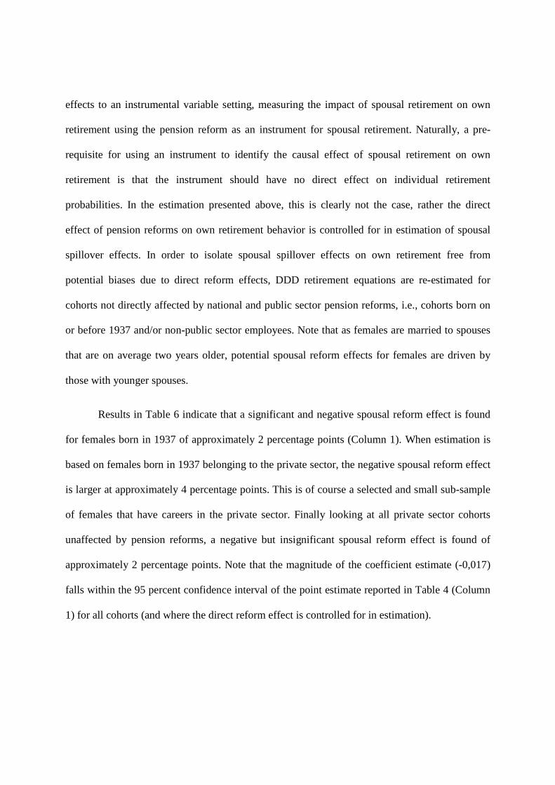
Results in Table 6 indicate that a significant and negative spousal reform effect is found
for females born in 1937 of approximately 2 percentage points (Column 1). When estimation is
based on females born in 1937 belonging to the private sector, the negative spousal reform effect
is larger at approximately 4 percentage points. This is of course a selected and small sub-sample
of females that have careers in the private sector. Finally looking at all private sector cohorts
unaffected by pension reforms, a negative but insignificant spousal reform effect is found of
approximately 2 percentage points. Note that the magnitude of the coefficient estimate (-0,017)
falls within the 95 percent confidence interval of the point estimate reported in Table 4 (Column
1) for all cohorts (and where the direct reform effect is controlled for in estimation).
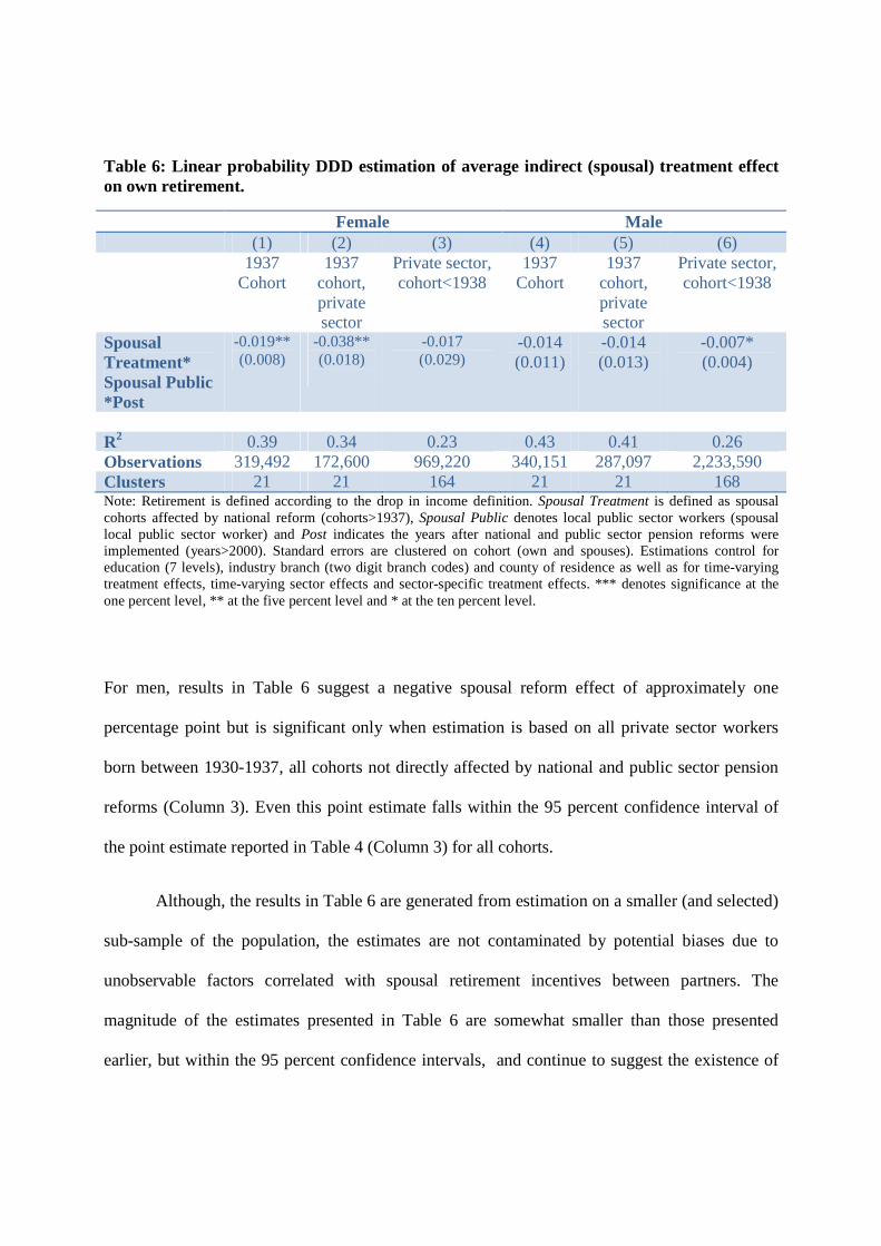
Table 6: Linear probability DDD estimation of average indirect (spousal) treatment effect on own retirement.
Female Male (1) (2) (3) (4) (5) (6) 1937
Cohort 1937
cohort, private sector
Private sector, cohort<1938
1937 Cohort
1937 cohort, private sector
Private sector, cohort<1938
Spousal Treatment* Spousal Public *Post
-0.019** (0.008)
-0.038** (0.018)
-0.017 (0.029)
-0.014 (0.011)
-0.014 (0.013)
-0.007* (0.004)
R2 0.39 0.34 0.23 0.43 0.41 0.26 Observations 319,492 172,600 969,220 340,151 287,097 2,233,590 Clusters 21 21 164 21 21 168 Note: Retirement is defined according to the drop in income definition. Spousal Treatment is defined as spousal cohorts affected by national reform (cohorts>1937), Spousal Public denotes local public sector workers (spousal local public sector worker) and Post indicates the years after national and public sector pension reforms were implemented (years>2000). Standard errors are clustered on cohort (own and spouses). Estimations control for education (7 levels), industry branch (two digit branch codes) and county of residence as well as for time-varying treatment effects, time-varying sector effects and sector-specific treatment effects. *** denotes significance at the one percent level, ** at the five percent level and * at the ten percent level.
For men, results in Table 6 suggest a negative spousal reform effect of approximately one
percentage point but is significant only when estimation is based on all private sector workers
born between 1930-1937, all cohorts not directly affected by national and public sector pension
reforms (Column 3). Even this point estimate falls within the 95 percent confidence interval of
the point estimate reported in Table 4 (Column 3) for all cohorts.
Although, the results in Table 6 are generated from estimation on a smaller (and selected)
sub-sample of the population, the estimates are not contaminated by potential biases due to
unobservable factors correlated with spousal retirement incentives between partners. The
magnitude of the estimates presented in Table 6 are somewhat smaller than those presented
earlier, but within the 95 percent confidence intervals, and continue to suggest the existence of
causal spillover effects in retirement behavior. If these point estimates are interpreted as the
reduced form effect of spousal pension reforms on own retirement behavior, the IV estimates of
spousal retirement on own retirement amounts to approximately 16 percentage points for women
and 6 percentage points for men.34 In comparison, OLS estimates of the correlation between own
retirement and spousal retirement is approximately 17 percentage points for females and 16
percentage points for males (in estimation controlling for birth year (own and spouses), sector of
employment (own and spouses), education, county of residence, branch and year fixed effects).
If the estimates reported in Table 6 are taken to represent the causal spillover effect for
the larger population, the magnitude of the effect suggests that the full impact of pension reforms
on retirement behavior, over and beyond the direct effects reported in Table 2, are under-
estimated by approximately 14 percent for females and 6 percent for males when spousal
spillover effects are not taken into account.35
7 Conclusions
This study exploits a recent Swedish pension reform to identify spill-over effects of a change in
spousal pension incentives on individual pension behavior. A difference-in-difference-in
difference identification strategy is used to estimate the effect on retirement probabilities of
having spouses treated by local public sector and national pension reforms in comparison to
34 Back of the envelope IV estimates are calculated using the reduced form estimate presented in Table 6 (Columns 3 and 6) and the first stage estimates presented in Table 2 (Columns 1 and 3) where the coefficient for females is taken to represent the first stage effect for wives and the coefficient for males is taken to represent the first stage effect for husbands. In other words the IV estimate for females is equal to : -0,017/-0,112 and for males: -0,007/-0,122. 35 Calculations depart from estimates of the direct reform effect presented in Table 2 and the spousal spillover effect presented in Table 6 for cohorts and sectors directly unaffected by pension reforms (Column 3 and 6): For females: -0,017/-0,122 and for males: -0,007/-0,112
those with spouses unaffected by these pension reforms, before and after pension reforms are
implemented.
Results indicate that pension reforms had a direct effect on retirement behavior due to
changes in own pension incentives and an indirect effect via changes in spousal retirement
incentives. Having a spouse affected by national and public sector pension reforms reduces
retirement probabilities after the reform is implemented in comparison to those with spouses
unaffected by reforms, by about 5-6 percentage points, controlling for the direct effect of the
pension reform on own retirement probabilities. Estimation that instead exploits variation within
spousal birth cohorts in public sector affiliation suggest a lower magnitude in spousal spillover
effects that varies across spousal birth cohorts.
Although our estimates of spousal spillover effects are large and potentially contaminated
by unobserved characteristics correlated with spousal retirement reforms, estimation on a sub -
sample of individuals belonging to cohorts and sectors that were not directly affected by national
and public sector pension reforms yields results indicating a smaller point estimate of the effect
of changes in spousal retirement incentives on retirement behavior of approximately 2
percentage points for females and 1 percentage point for males. Note that these estimates fall
within the 95 percent confidence intervals of the estimates on the full sample of cohorts where
direct reform effects were controlled for in estimation. If the smaller point estimates are taken to
represent the spillover effects for the larger population, the full impact of pension reforms on
retirement behavior are under-estimated by approximately 14 percent for females and 6 percent
for males when spousal spillover effects are not taken into account.
References:
An, Mark Y., Christensen, Bent Jesper and Datta Gupta, Nabanita, (2004), “Multivariate Mixed Proportional Hazard Modelling of the Joint Retirement of Married Couples” Journal of Applied Econometrics, Vol. 19, pp. 687-704.
Baker, Michael (2002), “The Retirement Behavior of Married Couples: Evidence from the Spouse’s Allowance” The Journal of Human Resources, Vol 37, No. 1 (Winter, 2002), pp. 1-34.
Blau, David M., (1998), “Labor Force Dynamics of Older Married Couples” Journal of Labor Economics, Vol. 16, No. 3, pp. 595-629.
Brown, Kristine M., and Laschever, Ron A. (2012). "When They're Sixty-Four: Peer Effects and the Timing of Retirement." American Economic Journal: Applied Economics, 4(3): 90–115.
Coile, Courtney, C., (2003), “Retirement Incentives and Couples’ Retirement Decisions” NBER Working Paper Series, Working Paper 9496.
Cullen, Julie Berry and Jonathan Gruber, 2000. Does unemployment insurance crowd out spousal labor supply?, Journal of Labor Economics 18(3):546-572.
Gelber, Alexander (2012) “Taxation and the Earnings of Husbands and Wives: Evidence from Sweden” Uppsala Center for Fiscal Studies Working Paper 2012:4.
Glans, Erik (2008), “Retirement Patterns during the Swedish Pension Reform” Department of Economics Working Paper 2008:9, Uppsala University.
Gustman, Alan, L. and Steinmeier, Thomas L., (2000) “Retirement in Dual-Career Families: A Structural Model” Journal of Labor Economics, Vol. 18(3), pp. 503-545
Hurd, Michael D., (1990), “The Joint Retirement Decision of Husbands and Wives” in Wise, David A. (Editor) “Issues in the Economics of Aging” University of Chicago Press. Johnson, Richard W. and Favreault, Melissa M. (2001), “Retiring Together or Working Alone: the Impact of Spousal Employment and Disability on Retirement Decisions” Center for Retirement Research, Boston College, CRR WP 2001-01. Kapur, Kanika and Rogowski, Jeannette (2007), 'The role of health insurance in joint retirement among married couples', Industrial and Labor Relations Review, 60 (3), pp. 397- 407.
Lazear, E. P. (1986), “Retirement from the Labor Force” in Ashenfelter, O. C. and Layard, R. (Eds.), Handbook of Labor Economics, , Elsevier B.V., Vol. 1: 305-356.
Lumsdaine, r. L. and Mitchell, O. S., (1999), “Economic Analysis of Reitrement” in Ashenfelter, O. and Card, D. (Eds.), Handbook of Labor Economics, , Elsevier B.V., Vol. 3C: 3261-3308.
Maestas, Nicole Anne, (2002), “Planning for Widowhood? Joint Retirement and the Allocation of Pension Income by Older Couples” PhD dissertation University of California, Berkeley.
Mastrobuoni, Giovanni (2009), “Labor supply effects of the recent social security benefit cuts: Empirical estimates using cohort discontinuities” Journal of Public Economics, Vol. 93, pp. 1224-1233.
Olsson, Martin and Skogman Thoursie, Peter (2010) “Insured by the Partner?” IFAU Working Paper 2010:3.
Palme, Mårten and Svensson, Ingemar (1999), “Social Security, Occupational Pensions and Retirement in Sweden” in J. Gruber and D. Wise (eds.) Social Security and Retirement around the World, University of Chicago Press.
Palme, Mårten and Svensson, Ingemar (2002), “Pathways to Retirement and Retirement Incentives in Sweden” in T. Andersen and P. Molander (eds.) Alternatives for Welfare Policy, 2003, Cambridge University Press: Cambridge.
Pozzebon, S. and Mitchell, O.S., (1989) “Married women’s retirement behavior”, Journal of Population economics, Vol. 2(1): 39-53.
Pozzoli, Dario and Ranzani, Marco (2009) “Old European Couples’ Retirement Decisions: the Role of Love and Money” Aarhus Department of Economics Working Paper 2009-2
Selin, Håkan (2011), “What happens to the husband’s retirement decision when the wife’s retirement incentives change?” Uppsala Center for Fiscal Studies, Working Paper 2011:8.
Sjögren Lindqvist, Gabriella and Wadensjö, Eskil (2006) “National Social Insurance – not the whole picture. Supplementary compensation in case of loss of income”, Ministry of Finance, Report for ESS 2006:5
Stancanelli, Elena G. F., (2012) "Spouses' Retirement and Hours Outcomes: Evidence from Twofold Regression Discontinuity with Differences-in-Differences" IZA Discussion Paper No. 6791.
Sundén, Annika (2006), “The Swedish Experience with Pension Reform” Oxford Review of Economic Policy, Vol. 22(1): 133-148.
Zweimüller, Josef, Winter-Ebmer, Rudolf and Falkinger, Josef, (1996), “Retirement of spouses and social security reform” European Economic Review, Vol. 40, pp. 449-472.
Appendix
Figures A1-A6: Retirement hazards by age, cohort and sector, females
Note: “kom1” denotes municipal employees and “other1” denotes private sector employees
0.1
.2.3
.4.5
.6.7
.8.9
1C
_re
t_dr
opin
c
45 50 55 60 65 70age
37 38
ret_dropinc woman kom1
0.1
.2.3
.4.5
.6.7
.8.9
1C
_re
t_dr
opin
c45 50 55 60 65 70
age
37 38
ret_dropinc woman other1
0.1
.2.3
.4.5
.6.7
.8.9
1C
_ret
_dro
pin
c
45 50 55 60 65 70age
38 39
ret_dropinc woman kom1
0.1
.2.3
.4.5
.6.7
.8.9
1C
_ret
_dro
pin
c
45 50 55 60 65 70age
38 39
ret_dropinc woman other1
0.1
.2.3
.4.5
.6.7
.8.9
1C
_ret
_dro
pin
c
45 50 55 60 65 70age
39 40
ret_dropinc woman kom1
0.1
.2.3
.4.5
.6.7
.8.9
1C
_ret
_dro
pin
c
45 50 55 60 65 70age
39 40
ret_dropinc woman other1
Figures A7-A12: Retirement hazards by age, cohort and sector, males
Note: “kom1” denotes municipal employees and “other1” denotes private sector employees
0.1
.2.3
.4.5
.6.7
.8.9
1C
_ret
_dr
opi
nc
45 50 55 60 65 70age
37 38
ret_dropinc man kom2
0.1
.2.3
.4.5
.6.7
.8.9
1C
_ret
_dr
opi
nc
45 50 55 60 65 70age
37 38
ret_dropinc man other2
0.1
.2.3
.4.5
.6.7
.8.9
1C
_re
t_dr
opi
nc
45 50 55 60 65 70age
38 39
ret_dropinc man kom20
.1.2
.3.4
.5.6
.7.8
.91
C_r
et_
dro
pin
c
45 50 55 60 65 70age
38 39
ret_dropinc man other2
0.1
.2.3
.4.5
.6.7
.8.9
1C
_re
t_dr
opi
nc
45 50 55 60 65 70age
39 40
ret_dropinc man kom2
0.1
.2.3
.4.5
.6.7
.8.9
1C
_re
t_dr
opi
nc
45 50 55 60 65 70age
39 40
ret_dropinc man other2
Figure A13: DDD estimation of a change in own pension incentives on own retirement probabilities (birth cohort*public*post interaction relative to 1937 cohort). Public Sector Employees defined as municipal and county workers only (no state employees).
-.1
5-.
1-.
05
0.0
5E
stim
ate
d c
oe
ffic
ien
t
1931 1933 1935 1937 1939 1941 1943 1945 1947 1949Birth year
DDD estimation of direct reform effect, males