spontaneously broken gauge theory in a gauge-independent path-dependent formalism

P H Y S I C A L R E V I E W D V O L U M E 1 8 , N U M B E R 4 1 5 A U G U S T 1 9 7 8

Sponttlneously broken gauge theory in a gauge-independent path-dependent formalism

Seichi Naito and Seizi Akahori Department of Physics, Osaka City Universiry, Sumiyoshiku, Osaka, Japan

(Received 9 June 1977)

In a gauge-independent path-dependent formalism, we quantize a local SO(3) gauge-invariant theory in which the triplet gauge bosons A ",a = 1,2,3) are interacting with a triplet of real scalar fields 4" ( a = 1,2,3). Especially in Rc gauges, we investigate the spontaneously broken case, by incorporating the boundary conditions for the Green's functions. Feynman rules for the Green's functions are derived and found to be the same as those prescribed by 't Hooft. Furthermore, we obtain the result of Lee and Zinn- Justin that Ward-Takahashi identities are the same for both symmetric and spontaneously broken cases. With the help of these identities and the massiveness of the Higgs particle, we can prove the gauge independence of the S matrix.

I. INTRODUCTION Lagrangian i s given by

In a ser ies of papers'-3 on the massless Yang- = -+[A7u(x)]2

Mills field,+ it has been clarified that many results 4 '(x) +g6y6~zj(x)$E (x)12 derived by ~ e y n m a n ' s path-integral method5 can be rederived by the field-theoretical quantization

- ~ P ~ [ ~ Y ( X ) I ~ - + A { [ $ ~ ( X ) I ~ ) ~ , (1.1)

scheme in a gauge-independent path-dependent where formalism. On the other hand, the spontaneously broken gauge theory (i.e., massive Yang-Mills field) has been extensively investigated and many interesting results have been obtained only by a path-integral method. However, various results should be critically checked because of the following situations: In applying a path-integral method to the theory with spontaneously broken symmetry, Matsumoto, Papastamatiou, and TJmezawa6 have emphasized the necessity of introducing a limiting prescription in the definition of the generating functional itself, in order t o incorporate boundary conditions specifying solutions of the field equations. Applying their method to spontaneously broken models of scalar fields (invariant under constant gauge transformation), they have derived correct Ward-Takahashi identities, which a r e different from those obtained without the limiting prescription. (Their results were la te r confirmed to be valid by Nakanishi7 in a purely field-theoretical way.) Since Lee and Zinn-Justin have used a generating functional without exp2icitly considering the boundary conditions, we cannot uncritically be- lieve their conclusion8 that Ward-Takahashi iden- t i t ies in the spontaneously broken case a r e the same a s those in the symmetric case. In th is pap- e r , we shall rederive various results obtained by a Feynman path-integral method by using a field- theoretical quantization scheme in a gauge-independent path-dependent formalism.

For concreteness we consider a local SO(3) gauge-invariant theory in which the triplet gauge bosons A;(a = 1 , 2 , 3 ) a r e interactingwith a triplet of real scalar fields @a ( a = l , 2 , 3). Our classical

[ ~ n Secs. I and 11, a tilde denotes classical quanti- t ies . Throughout this paper, we use the following notations: Greek indices p, v, p, a, @, w (Roman indices i, j, k, I) denote components in ordinary space and vary from 1 to 4 (3). Other Greek indices denote components in isotopic space and vary f rom 1 to 3. Repeated indices a r e to be summed over.] F i rs t we introduce the path-dependent functions va7(x; P) by

- %

va,(x; m =a,, +ge7&, J; d t , , ~ ; ( { ) ~ ~ ~ ( [ ; P!),

(1.2) where P i s an arbitrary path starting from m and ending at x. Then the path-dependent p's and 6's defined by

E u ( x ; P) Va7(x; ~ l . 7 ; ~ (4 , bN(x; P) = v,,(x; P)$Y(x) ,,

(1.3) and

q6cy~ ; P) = vaY(x; p)[6 ysa; + g ~ y , 6 i i ~ ( ~ ) ] J6(x)

a r e knowng" to be gauge independent. In Sec. 11, our classical fields 2, 6, and D,b

a r e quantized into quantum fields F, +, and D,@ by imposing the equal-time commutation relations (cR's). In order to make complete our description of the quantum system, we also give fundamental. equations among the quantized fields. In Sec. JII, we construct the covariant Green's functions by suitably combining the time-ordered products of the quantized fields. Fundamental equations to-

18 - S P O N T A N E O U S L Y B R O K E N G A U G E T H E O R Y I N A . . .

gether with CR'S among the quantized fields lead to an infinite number of equations among the covariant ree en's functions. With the help of these equations, we investigate in Sec. IV the case when local gauge invariance i s spontaneously broken. We show how R E g a ~ g e s ' ~ ' " can be introduced in our formalism. Incorporating boundary conditions, we derive in R E gauges the same Feynman ru les a s those given by 't Hooft.lo Furthermore, we show in Sec. V the reason (in our formalism) why the result of Lee and Zinn-Justin8-that Ward-Taka- hashi identities a r e the same for both symmetric and spontaneously broken cases-is correct . With the help of these identities and the massiveness of the Higgs particle," we can prove the gauge independence of the S matrix.

11. QUANTIZATION IN A GAUGE-INDEPENDENT PATH-DEPENDENT FORMALISM

The derivation of the Poisson brackets between gauge-independent path-dependent 3's' 6's and D44's proceeds in much the same way a s for the mass less Yang-Mills field,' so that we shall only sketch the derivation.

We consider the Lagrangian

In (2.1) and hereafter, the covariant derivatiz,e op- e_uution D", on the path-dependent quantities Q(x; P) i s defined by

Q(x+dx,; P + d P ) - Q(x; P) I l iG(x ; P) 5 l im dx,

9 d x p - o

where the path P + d P i s obtained from P simply by giving it an extension of magnitude dx, in the p direction. Then we have from (1.3), (2.2), and (1.2)

o'pQB(y; PI) = Vgy(y; P ' ) ( Y ~ D Y ~ / ~ ) ~ ~ ( Y ) (2 .3)

with

(riD',l6) = 6,,8., +gc,,dE,(y).

In a way similar to that in which we obtained (11) and (12) in Ref. 2, the variational principle

leads to

o=E,,,,D;E;,C~;P~),

and = D : ~ D ~ a b ; p x ) ~ - 112g~b; pX) - X [ ~ ~ ( X ; P , ) I ~ Z ~ ( ~ ; P , ) + E ~ ~ , B ~ ~ ( x - Y )

+ €,[6,,a:a4(x -Y) -g€,B,~:Cz-;~,)64(x-y)l,

with

and2

D ~ ~ ~ C ~ ; P , ) = ~ ~ ~ ~ C ~ ; P , ) - g f . a 7 6 ~ ~ ( x ; ~ x ) 6 6 b ; ~ x ) , (2.8)

where G a i s any one of the E;,'s ga ' s , and D , X ~ ~ ' S . In deriving (2.4)-(2.8), we prepared2 any one set of curves which satisfies the condition that there exists in the s e t only one curve passing through an arb i t ra r - ily fixed point x in spacetime, and took the path along the above-mentioned curve. Since the path so de-

1232 S E I C H I N A I T O A N D S E I Z I A K A H O R I 18 -

fined is uniquely determined by the end point x , i t is denoted by P, in (2.4)-(2.8). Hereafter we t r e a t the special c a s e when the t i m e coordinate of any point on P, is the s a m e (Ge., equal to x,).

Hereaf te r we consider D , x ~ " ( ~ ; P , ) a s independent fields, a s well a s F ~ , ~ ; P J and ga(x;p,) . Then the fundamental equations a r e

and those obtained by substituting (2.8) other than (2.9) into (2.4)-(2.6). The i r solutions [ ~ ~ , ~ ; P , ) ] , , , , [~"(X;PJ]~, , , and [D,X$"(X;P~],,, can be obtained in power expansions of E,, E,, and c,, and they a r e denoted by

[ Q " ~ ~ ; P J ~ , . ~ = ~ " ( ~ ; P , ) + ~ ~ ~ ~ ~ ~ , ~ , ~ , ~ " L . ; ~ ~ ) + ~ , ~ , ~ , ~ ~ , ~ ~ B " ~ ~ ; P , ) + ~ ~ ~ ~ ~ ~ ~ ~ ~ ~ ~ ~ , ~ " ~ : P , ) + O k 2 , c I t 2 , . . .) ,

where 6" is any one of the $~,'s, Gays, and ~ ~ 6 " ' s . In the neighborhood of x,=y,, explicit expressions of the right-hand s ide of (2.10) a r e given by

D E B ( ~ ~ ~ ~ ) Q ~ G ; ; P ~ ) - ~ E ~ ( ~ ; P ~ ) B a ~ ; ~ , ~ ~ ~ x , - ~ , ~ + i [ ~ ~ ~ ; ~ , ~ , ~ 6 ~ ~ ; ~ y ~ I ~ ~ o - ~ O ~ , (2.11)

where

[ F : ~ ; P ~ , F : ~ ( Y ; P ~ ) ~ = ~ € . ~ , F ~ ~ ~ ; P ~ l x d z ~ 6 3 ~ - 7 ) P,

and a l l other di;Q9s than (2.22) and (2.23) a r e equal t o zero. If we consider F ' s , a's, and D,@'s i n (2.12)- (2.21) a s quantized fields operating on the Hilbert space, the P e i e r l s rule13 says that (2.12)-(2.21) a t x, = y o a r e the equal-time commutation relat ions (CR's). The quantized f ie lds in consideration a r e charac te r - ized by CR's (2.12)-(2.21) and fundamental equations

F;,(~;P,) =-F& b;P,!,

o =D:F,o,(x;P~ - g c , 6 y $ { @ 6 b ; ~ , ) , ~ ~ @ Y G ; ; ~ X ) ) ,

o = E ,,,, D,xF;,G~;P,),

o =D; D;@"(X; P,) - g2@"(x ;~ , ) - h[@'(x; p,)IZ@"(x;PX),

S P O N T A N E O U S L Y B R O K E N G A U G E T H E O R Y I N A . . . 1233

and

D,x+"G~; P,) = a,x+aClc;P,) -gc .,,$ {~4Gc;p,) , @ 6 C r ; ~ , ) ? , where we have used shorthand notations

D;F;,(x;P,)= a ; ~ ; , G r ; P,) - ~ E , , , ~ { ~ , ' G ~ ; P , ) , F ~ , ( ~ ; P , ) ) ,

~ ~ 9 " G c ; i P,) = a;@"k;~,) - ~ E ~ ~ ~ B ; ( ~ ; P , ) @ ~ ~ ; P , ) ,

D:D:@"(X; P,) = B:[D:@~(x;P,)] -g€ .,,+{~,7(x;p,), D , x @ ~ ( ~ ; P , ) ) ,

D;D;@'&; ~ , ) [ ~ , , a ; - g ~ ~ ~ ~ ~ ~ b ; ~ , ) 1 [ 6 ~ ~ a ; - g c y , e ~ ~ b ; ~ r ) I @ E b ; P ~ )

with

{P,Q}=P - Q + Q .P

and

So long as we start f r o m (2.12)-(2.21) and (2.24)-(2.28), we do not need any other thing for the quantized fields F , 9 , and D,9. [~ncidentally we can prove consistency among (2.12)-(2.21) and (2.24)-(2.28) in much the same way as we did2 in the massless Yang-Mills field.]

111. COVARIANT GREEN'S FUNCTIONS

In order to investigate our quantum system (2.12)-(2.21) and (2.24)-(2.28), i t i s more convenient to treat the (covariant) Green's functions

( O I T * { F ; , ( ~ ; P ~ . . . F : , ( ~ ; P , ) + ~ ( V ; P,). - - 9 ° ( u ~ ; P w ) ~ ~ @ E ( u ; ~ , ) ~ . .D:@~(z;P,)}Io) (3.1)

than the noncovariant time-ordered products

(o)T{F;,(x;P,) . . . F ; ~ ( ~ ; P J @ ~ ( z I ; P , ) - . + 6 ( ~ ; ~ w ) ~ : @ E ( ~ ; ~ , ) . . . D : @ ~ C ~ ; P , ) } ~ O )

The general definitions o f (3.1) in terms of (3.2) may be easily imagined f r o m the following special example: The two-point covariant Green's functions (3.1) are the same as the corresponding (3.2), except for

(0 I T * { F , ~ ( X ; P , ) F , B , ( ~ ; P , ) ) ~ O ) ~ (O/T{F:G~;P,)F,B,(Y;P~)~~~)-~~.~~~,~~(X-Y) and

(O I T * { D ~ @ ~ ( x ; P , ) D : + ~ ( ~ ; P,)} 1 0 ) - (0 I T{D;@~(x ;P , )D:@~(Y ;P,)} 10) - i b a ~ b 4 ( x - Y )

The reason why we call (3.1) covariant Green's functions i s that our (2.12)-(2.21) and (2.24)-(2.28) are found to give the infinite set of covariant differential equations among (3.1). In order to express these equations compactly, we introduce Mandelstam's operators1 f, 6 , and D,6 acting on a linear space of the covariant Green's functions by the definition

Then our results can be expressed as follows2:

E .,,, D,xF;,G~;P,)=o, and

O = [ D ; D ; & ~ ( X ; P , ) - p 2 6 0 L ( x ; ~ , ) - A ( & ~ ( x ; P , ) ) ~ & ~ ( x ; P , ) - i ~ ~ ( x ; p , ) ] l G ) ,

where

1234 S E I C H I N A I T O A N D S E I Z I A K . 4 H O R I

and

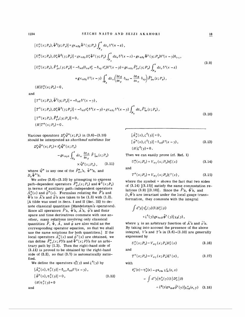
Various opera tors D;~*(.Y;P,) in (3.6)-(3.10) [ A ~ ( ~ ) , c ~ ( Y ) ] = 0 , should be interpreted as shorthand )zotations f o r

[Ga(x), LS(4)] =6,964(x - J ) , (3.13) D;@(x; P,)= a;gU(x; P,)

(HIc ' (Y)=o.

Then we can easi ly prove (cf. Ref. 1)

U::(s;P,) = V,, (.x;P,)qL ( x )

and where Qu i s any one of the @r,'s, ga's, and D , ga's. T ~ ( ~ ; P , ) = vay (x;P,)LY(.x), (3.15)

We solve (3.6)-(3.10) by attempting t o %xpress path-dependent opera tors F;,(.x; P,) and 9, (x ; P,) in t e r m s of auxiliary path-independent opera tors x;(x) and Ja (x) . Formulas relat ing the 2's and 4's to A's and 5's a r e taken to be (1.3) with (1.2). [A tilde was used in Secs. I and I1 (Sec. 111) to denote classical quantit-ies (~an$elsta_m's operators) . Since a l l opera tors F's, a's, A'S, 9's and their space and t ime derivat ives commute with one an- other, many relat!ons inv_olving only c lass ica l quantities F, a, A , and q, a r e a l s o valid a s the corresponding operator equation, s o that we shal l u s e the s a m e notations fo r both quantities.] If the local opera tors A:(x) and $"(x) a r e obtained, we can define F;,(x;P)'s and g a ( x ; P)'S for an a rb i - t r a r y path by (1.3). Then the right-hand s ide of (3.11) i s proved to b e obtained by the right-hand s ide of (2.2), s o that (3.7) i s automatically sa t i s - fied.

We define the opera tors q;(y) and by

[ A ~ ( X ) , V ~ ( ( V ) I = ~ ~ , ~ , ~ ~ ~ ( ~ - y ) ,

[$*(d ,~;(4 ' )] = o , (3.12)

( H ~ V ; ( ~ ) = O and

where the symbol = shows the fact that two s ides of (3.14) [(3.15)] satisfy the s a m e commutation r e - lations (3.9) [(3.10)]. Since the g's, G's, and ~ ~ 6 ' s a r e invariant under the local gauge t rans - formation, they commute with the integral

/d4).[n: ( - Y ) ( ~ I D : ~ I 6)

+ C ~ ( Y ) ~ ~ ~ E B ~ ' (Y ) ] xB(Y)

where x i s an a r b i t r a r y function of A's and o's. By taking into account the p resence of the above integral, V's and T's in (3.6)-(3.10) a r e generally expressed by

u ~ ( x ; P,) = Vay (x;P,)Bt (N) (3.16)

and

T"(x;P,) = Vay ( X ; P , ) ~ ~ ( x ) , (3.17)

with

~ ~ ( x ) = u ~ ( x ) -gEY6E x ~ ~ ( x , x )

- j + d 4 ~ [ n 6 ( y ) ( 6 / ~ : 10)

+ S 6 ( ~ ) ~ ' 6 E , & E ( y ) ] ~ ~ ~ ( ~ , y ) (3.18)

18 P P O h T A V L O U S 1 , Y B R O K B N G A I I G I . , T H E O R Y I U A . . . 1235 -

and

[ ' ( x ) = ~ ~ ( x ) - ~ E ~ G E ~ ~ ~ ( x , X )

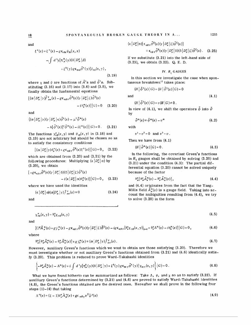
If we substitute (3 .21) into the left -hand s ide of (3.23): we obtain (3.22). Q. E. D.

+ L 6 ( y ) g c 6 e B c ~ E ( ~ ~ ) j i , y B ( x , ~ ) IV. R , GAUGES

(3.19) In th i s section we investigate the c a s e when spon-

where x and $ a r e functions of A ' s and 6's. Sub- taneous breakdowni2 takes place: stituting (3 .16) and (3.17) into (3 .6 ) and (3.8)' we

(I{ / $ ' ( X ) / G ) = (H / G " ( x ) ~ G ) = o finally obtain the iundamental equations

and [ ( ( a ! ] ~ ; I-/$:,,(Y) - ~ E ~ ~ ~ ~ ~ ( X ) ( - Y I D : / c ) ~ ' ( x - ) (4.1)

(11 / J 3 ( x ) l ~ ) = U ( H / G ) # 0 . - i @ : ( x ) l l G ) = o (3 .20)

In view of (4.1), we shift the opera tors 6 into 3 and

{ ( a I D : / Y ) ( Y I D : j t ) J s ( x ) - f i 2 6 0 ( x )

- h [ $ ( x ) ] ' l G a ( x ) - i t : L I ( x ) ) / ~ ) = O . (3.21) with

The functions x,YB(x, y ) and $,,(x, 31) in (3.18) and vi = L : ~ = 0 and t13 = 21 . (3.19) a r e not a r b i t r a r y but should b e chosen s o a s

Then we have f r o m (4.1) to satisfy the consistency conditions

( H J + ~ ( x ) I G ) = o . [ ( a I u ~ / Y ) % , Y ( x ) + ~ ~ ~ ~ ~ ~ ~ ( x ) [ ~ ( x ) ] / ~ ) = O , (3 .22)

In the following, the covariant Green 's functions which a r e obtained f r o m (3.20) and (3.21) by the in R E gauges shall be obtained by solving (3.20) and following procedures: Multiplying ( c ID: / a ) by (3 .21) under the condition (4.3): The part ia l dif- (3.20)' we obtain ferent ial equation (3.20) cannot b e solved uniquely [ - g c E B y 6 B ( ~ ) ( ~ / I ) ; / 6 ) ( f i I ~ : j i - ) & ' ( ~ ) because of the factor

where we have used the identities and (4.4) originates f r o m the fact that the Yang- Mills field A:(x) is a gauge field. Taking into a c -

( E / ~ : / a ) ( f f I q ' / Y ) ~ : , ( x ) = o (3 '24 ) count the ambiguities resul t ing f r o m (4 .4 ) , we t r y and t o solve (3 .20) in the f o r m

and

where

a;[a;A;(~) - a ; A ; ( ~ ) ] + ~ j ; ( x ) = ((a! ID: l ~ ) ? l , ( x ) . (4.7)

However, auxiliary Green 's functions which we want to obtain a r e those satisfying (3.20). Therefore we mus t investigate whether o r not auxiliary Green's functions obtained f r o m (3.21) and (4.6) identically s a t i s - fy (3.20). This problem is reduced t o prove Ward-Takahashi identities

What we have found hitherto can be summar ized a s follows: Take A , $, and x s o a s t o sat isfy (3.22). If

auxiliary Green's functions determined by (3.21) and (4.6) a r e proved to satisfy Ward-Takahashi identities (4.8)' the Green's functions obtained a r e the des i red ones. Hereafter we shall prove in the following four s t e p s ( 1 ) - ( 4 ) that taking

S E I C H I N A I T O A N D S E I Z l A K A H O R I

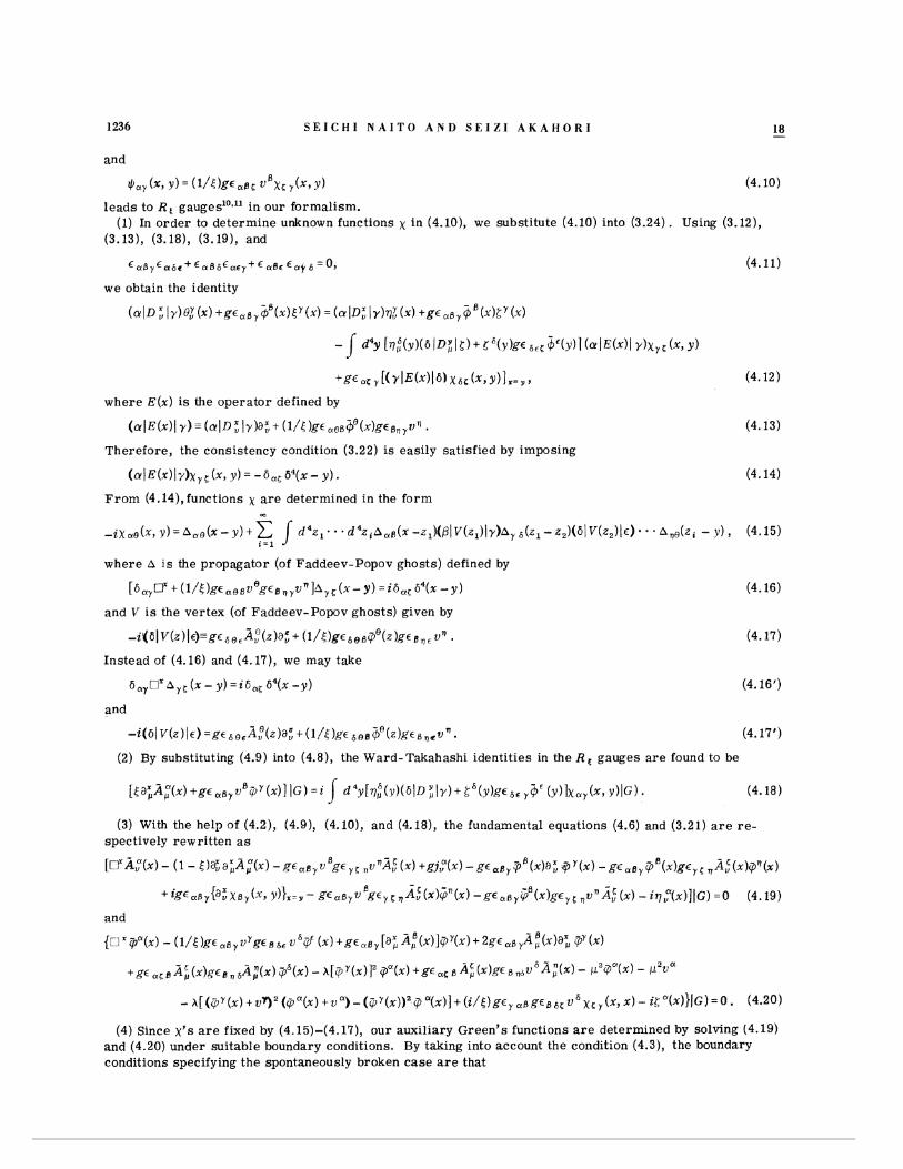
and

leads to R E gauges10-" in our formalism. ( 1 ) In o r d e r to determine unknown functions x in (4.10), we substitute (4.10) into (3 .24) . Using (3.12),

(3.131, (3 .18) , (3.19), and

E a B y E u 6 ~ + E a ~ & E a e Y + E a ~ e E a ) . s = 0 ,

we obtain the identity

- 5 ? y ( ~ I D : I Y ) @ , Y ( X ) + R E , B ~ O (XI( (XI = ( ~ I D : / Y ) ~ , ! ( x ) + ~ E , ~ ~ $ J ' ( X ) C Y ( X )

- d4y [ T I , ? ( Y ) ( ~ / D ; I c ) + C ' ( V ) & ? C ~ ~ ~ $ ' ( Y ) ~ ( a l ~ ( x ) l Y ) X ~ ~ ( X , Y )

' g ~ a , y [ ( Y I E ( ~ ) ~ ~ ) X ~ < ( X , Y ) ~ X = ~ , (4.12)

where E ( x ) i s the opera tor defined by

( f f l E ( ~ ) I Y ) - ( ( Y I D ~ I Y ) ~ : + ( ~ / < ) ~ E . ~ B $ ' ( X ) R ~ B ~ ~ V ' . (4 .13)

Therefore, the consistency condition (3 .22) i s easily satisfied by imposing

( a l E ( x ) I ~ ) ~ , ~ ( ~ , v ) = - 6 , , 6 ~ ( x - y ) . (4.14)

F r o m (4.14),functions x a r e determined in the f o r m

where A I S the propagator (of Faddeev-Popov ghosts) defined by

e [ 6 , , 0 + ( 1 / < ) g c a R ~ u ~ E ~ , , ~ U ' ~ ] A ~ ~ ( X - Y ) =i6,( 6 4 ( ~ - Y ) (4.16)

and 1.' i s the vertex (of Faddeev-Popov ghosts) given by

- i ( 6 1 V ( z ) I t ) = ~ t ~ ~ ~ A f ( z ) a : + ( 1 / < ) g t 6 0 B @ ( z ) s B r l r u l ) . (4.17)

Instead of (4.16) and (4 .17) , we may take

6 , y O r ~ y C ( ~ - y)=i6,< ~ S ~ ( x - y ) (4.16')

and

-i(al T I ( Z ) ~ E ) = g ~ ~ ~ ~ A v B ( z ) a : + ( l / < ) g ~ & ~ B $ ' ( ~ ) R E B , ~ V " . (4.17')

( 2 ) By substituting (4.9) into (4 .8) , the Ward-Takahashi identities in the R, gauges a r e found to be

( 3 ) With the help of (4.21, (4.9), ( 4 . 1 0 ) ~ and (4.18), the fundamental equations (4.6) and (3.21) a r e r e - spectively rewri t ten a s

[ ~ ; i , " ( x ) - ( 1 - t ) % a ; A f ( x ) - g c . ~ , u ~ g ~ ~ ~ ,cn;1,S(x) +gj:(x) - g ~ a s y q B ( ~ ) a : q u ( x ) - g ~ a B y + e ( ~ ) g ~ y I : ,,Avt(x)q9(x)

B - B ~ i ~ E a ~ y { a ~ ~ B y ( x ~ ~ ) ~ x = y - g ~ a ~ y ~ ~ ~ y ~ R ~ ~ ( ~ ) ~ n ( ~ ) - ~ ~ a ~ y ~ ( ~ ) g ~ y 6 r j ~ " ~ ~ ( ~ ) - i 7 7 ~ ( X ) ] ~ ~ ) = ~ (4.19)

and

{?"$*(x) - ( ~ / ( ) & ' E ~ B ~ u ~ ~ € ~ 5~ c'$' ( x ) + g t a e y [ a t A , B ( x ) ] ~ Y ( x ) + 2 g ~ a ~ y A : ( ~ ) a ; qy ( x )

+ g t a c s A : ( x ) q ~ g n 6 A ~ ( ~ ) q 6 ( x ) - ~ [ l i ) Y ( x ) ] ~ g ~ ( x ) +geaC B A : ( X ) ~ E B ~ U ~ A ~ ( X ) - p Z l i ) a ( ~ ) - 1 ~ ~ 2 ) ~

( 4 ) Since X'S a r e fixed by (4.15)-(4.17)' our auxiliary Green 's functions a r e determined by solving (4 .19) and (4 .20) under suitable boundary conditions. By taking into account the condition (4 .3) , the boundary conditions specifying the spontaneously broken c a s e a r e that

18 4

S P O N T A N E O U S L Y B R O K E K G A U G E T H E O R Y I K A . . . 1237

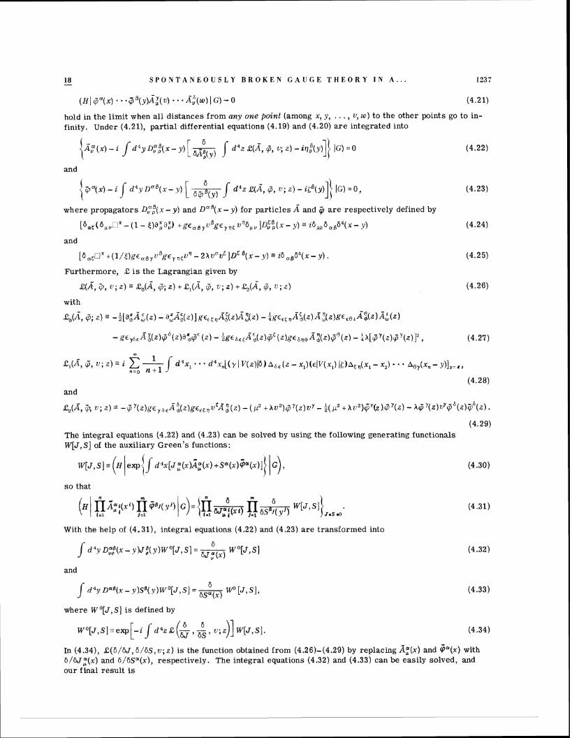
hold in the limit when all distances from any one point (among x, y, . . . , U , w) to the other points go to in- finity. Under (4 .21) , partial differential equations (4 .19) and (4 .20) a r e integrated into

and

where propagators D::(x - y) and D a a ( x - y) for particles A and 3 a r e respectively defined by

[ 6 , c ( 6 , , J x - ( 1 - 5 ) a ; d : ) + g c a g y l a g c y , , v ~ 6 , , ] ~ ~ ~ ( ~ - j ~ ) ~ 26, ,6a864(x- j ) (4 .24)

and

[ 6 , 5 L J X + ( l / [ ) g ~ , B y l Rgcy,,t~" ~ W ~ U ' ] D ~ 8 ( c - ~ l ) a 2 6 , B 6 4 ( ~ - y ) . (4 .25)

Furthermore, C i s the Lagranglan glven by

qe(A, G, r ; z ) = ~ ~ ( 2 , 5; z ) + c,(A, q , '; z ) +cJA, q, r ; 2 ) (4.26)

with

q; Z ) 5 -$[a; i l : (z) - a:A;(z)] K%,,A,S(~)IILjX~) - $Y~,~qA~(~)~;(z)g~fR,A$(~)A~(z)

- 1 &,(A, q, r ; 2 ) 2 E -/ d 4 x 1 . . . d4*,,[(yI v ( z ) I ~ ) A ~ , ( z - X , ) ( ~ / V ( X ~ ) I ~ ) A ~ , ( X , - x z ) . - A ~ ~ ( x ~ - ~ ) 1 ~ . . ,

n.0 11+1

(4 .28) and

sz(A, $, c ; 2 ) - ~ Y ( Z ) ~ E ~ ~ ~ A ~ ( Z ) ~ E ~ ~ ~ V ~ A ~ ( Z ) - (jl' + A U ~ ) ~ ~ ( Z ) D Y - $(112 + A Z 2 ) ~ Y ~ ) q Y ( ~ ) - x ~ ~ Y ( z ) ? ? Y ~ ~ ( z ) ~ $ ~ ( z ) .

(4 .29) The integral equations (4.22) and (4 .23) can be solved by using the following generating functionals W [ J , S ] of the auxiliary Green's functions:

s o that

With the help of (4,311, integral equations (4.22) and (4.23) a r e transformed into

and

where W ' [ J , S ] i s defined by

In (4.341, C ( 6 / 6 J , 6 / 6 S , z 1 ; z ) i s the function obtained from (4.26)-(4.29) by replacing A;(x ) and @ ( x ) with 6 ! 6 ~ ; ( x ) and 6 / 6 s U ( x ) , respectively. The integral equations (4.32) and (4.33) can be easily solved, and our final result is

1238 S E I C I I I N A l T O A N D S E I Z I A K A H O R I - 18

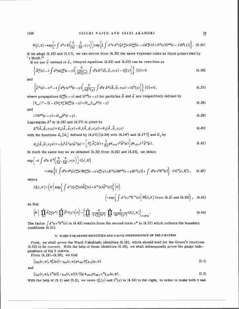
If we adopt (4.16) and (4.171, we can der ive f r o m (4.35) the s a m e Feynman r u l e s a s those prescr ibed by ' t ~ 0 0 f t . l ~

If we use 6 instead of @, integral equations (4.22) and (4.23) can be rewri t ten a s

and

where propagators a,":(x - JI) and a a 0 ( x - y ) fo r par t ic les A and 6 a r e respectively defined by

[ 6 i ( y ~ x - ( 1 - r ; ) a ; a y " ] ~ , " , B ( ~ - y ) = i 6 p p 6 a 6 6 4 ( r - y ) (4.38)

and

0 ~ 5 3 ~ ~ 0 : - y ) = i6,,6"(x -y ) . (4.39)

Lagrangian BS in (4.36) and (4.37) is given by

~S(A,$,0;z)=~o(ii,~;~)+~l(Z,~,tJ;z)+~3(~,~,2);z) (4.40)

with the functions 2, [Z , ] defined by (4.27) [(4.28) with (4.16') and (4.17')] and Z , by

In much the s a m e way a s we obtained (4.35) f r o m (4.22) and (4.23), we obtain

where

d ~ ~ ~ x ~ ~ x ) + ~ " ( x ) ~ ' ( x ) ]

( = e x p [ l d ' x t l a ~ .(I)] ~ J , K ] f r o m (4 .2) and (4.30) , (4.43)

s o that

The factor J ~ ' X V ~ K ~ ( X ) in (4.42) resu l t s f r o m the second t e r m v u in (4.37) which ref lects the boundary conditions (4.21).

V. WARD-TAKAHASHI IDENTITIES AND GAUGE IIVDEPENDENCE OF THE S MATRIX

Fi rs t , we shal l prove the Ward-Takahashi identities (4.18)' which should hold for the Green's functions (4.35) t o b e cor rec t . With the help of these identities (4.18), we shall subsequently prove the gauge independence of the S matrix.

F r o m (4.18)-(4.20), we find

[ ~ a e ( v , to), ~ E ( z l ) ] = X S ~ ( V , Z L ) ~ ~ ~ . O ~ ~ : X Y C ( ~ J , 20) (5.1)

and

[x,c(z', w ) , 5'(21)] = &(us u ) ( l / t ) g ~ , o ~ g ~ ~ ~ z ~ ' x ~ ~ ( u , M ) . (5 .2 )

With the help of (5 .1) and (5 .2 ) , we move q 6 , ( ~ ) and 6 ' ( y ) i n (4.18) to the right, i n o r d e r to make both q and

18 - S P O N T A B E O L S L Y B R O K E N G A U G E T H E O R Y I N A . . . 1239

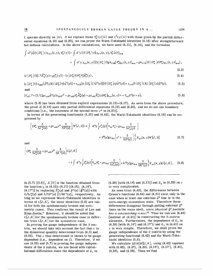
6 operate direct ly on (G). If we replace these $ ( y ) / G ) and L ~ ( ~ ) / G ) with those given by the par t i a l d i f fe r - ential equations (4.19) and (4.20)' we can prove the Ward-Takahashi identities (4.18) after s t raightforward but tedious calculations. In the above calculations, we have used (4. l l ) , (4.14), and the fo rmulas

(Y ID; 16) 666C[6B(.Y)(S 1% (77)6q(~)1 ' ~ y a e [ ( ~ 1 % I s ) ~ ' ( Y ) I [ ( ~ ID: 1 ~ ) 6 ~ ( ~ ) 1 + Cye6(6 I D ; 1 ~ ) ( < I D ; I v ) ~ ~ ~ J ) , (5.5)

and

1 6 y ~ ~ y + ( 1 / ~ ) g t ~ ~ e 6 ' b ) E o @ ~ - g t y B ~ a ; ~ ~ ( ~ ) -g tyB6~&(y)a ; ]XOLY(~, Y ) = - bOL6b4(x -y), (5.6)

where (5.6) has been obtained f r o m explicit expressions (4.15)-(4.17). As seen f r o m the above procedure, the proof of (4.18) u s e s only part ia l different ial equations (4.19) and (4.20), and we d o not use boundary conditions [i.e., the exis tence of the second t e r m vOL in (4.37)].

In t e r m s of the generating functionals (4.35) and (4.42), the Ward-Takahashi identities (4.18) can b e ex- p ressed by

6 + s%)gEa.,[v'+ x a i x , r )w[J , SI

and

In (5.7) [(5.8)], X [Y] is the function obtained f r o m the function x in (4.15)-(4.17) [(4.15), (4.16')' (4.17')] by replacing A:(%) and &OL(x) [qOL(x)] with 6/6J;(x) and 6/6SOL(x) [ 6 / 6 ~ ~ ( ~ ) ] , respectively. As long a s we represen t Ward-Takahashi identities in t e r m s of G[J,K], the s a m e identities (5.8) a r e valid f o r both the spontaneously broken and sym- met r ic cases . T h i s confirms the resul t of Lee and Zinn- ust tin.' However, i t should b e noted that G[J, K] f o r the spontaneously broken c a s e is different f r o m C[J,K] f o r the symmetr ic case.

In proving the gauge independence of the S ma- t r ix , we should take into account the fact that v is the dynamical quantity determined f r o m (4.3) and (4.35). The v thus determined is shown t o be gauge dependent (i.e., dependent on t). Therefore, i f we use (4.35) and (5.7) in proving the gauge independence of the S matr ix, we a r e faced with calcul- lational difficulties s ince the dependence of C, in

(4.28) [with (4.16) and (4.17)] and S., in (4.29) on u is very complicated.

As seen f r o m (4.43), the differences between Green 's functions (4.44) and (4.31) exis t only in the c a s e when a t l eas t one external q3 l ine is in the zero-energy-momentum state . Therefore these differences disappear through putting external q3 l ines on the m a s s shell, since physical q3 par t ic le has a norzvanishing mass.12 Thus we c a n use (4.44) [instead of (4.31)] in constructing the S-matr ix elements. Fur thermore , the dependence of C , in (4,28) [with (4.16') and (4.17')] and C, i n (4.41) on v is very simple. Therefore , we shal l prove the gauge independence of the S mat r ix by using the generating functional (4.42) and the Ward-Taka- hashi identities (5.8).

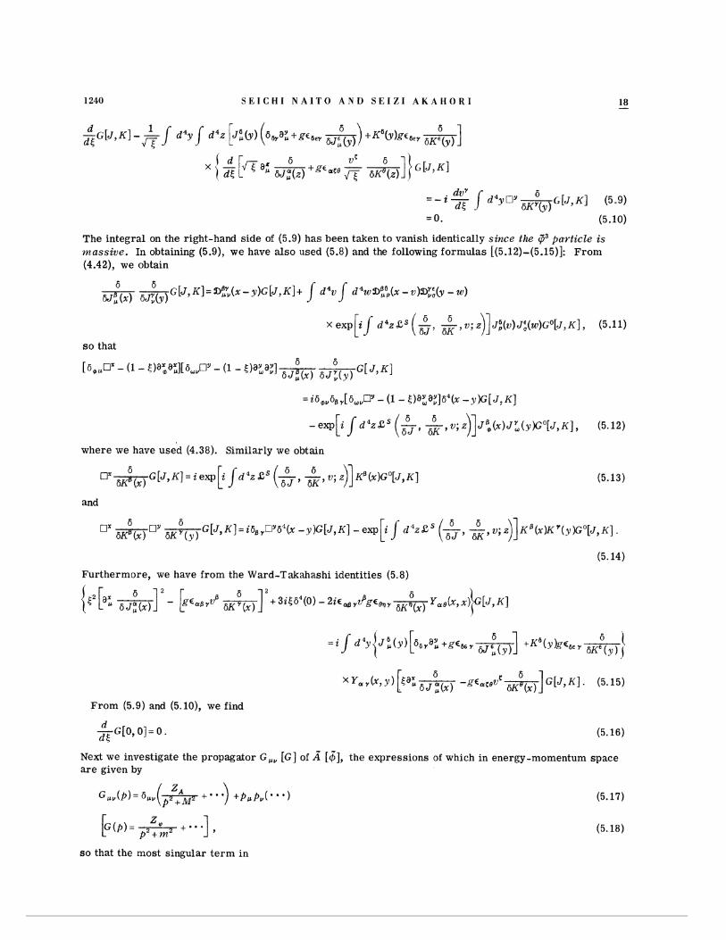
We calculate ( d / d < ) ~ [ J , K], using (4.42) together with (4.40), (4.27), (4.28)- (4.160, (4.17'), (4.41), (4.38), and (4,39). Then we find

1240 S E I C H I N A I T O A N D S E I Z I A K A H O R I

The integral on the right-hand side of (5.9) has been taken to vanish identically s ince the q3 particle i s n t a s s i v e . In obtaining (5.9), we have also used (5.8) and the following formulas [(5.12)-(5.15)]: From (4.42), we obtain

6 x enp[i/ d 4 r g s ($. = , v ; z)] J ~ ( u ) J : ( ~ ) G Q [ J , K ] , (5.11)

s o that

[6,,cX - ( 1 - [)ax,a;][6,,0~ - ( 1 - <)ay ,a;] 6 6

6 J ; ( x ) 6 J L ( y ) G[ J , K l

=i6,,6,y[6,,0y - ( 1 - <)aLa:]64(x - y ) G [ J : ~ ]

- e x p [ i ~ d ~ z ~ ~ isj-. & , ~ ; ~ ) ] J B , ( X ) J : ( ~ ) G ~ [ J , K ] , (5.12)

where we have used (4.38). Similarly we obtain

OX 6 6

~ ~ ~ u ( ~ ) G [ J , K I = ~ ~ w [ ~ ~ ~ ' ~ ~ ~ ( ~ , i . , , u ; z ) ] ~ ( x ) G O I J , K l

and

OX 6

0'- G [ J , K ] = i 6 , y D y 6 4 ( x - Y ) G [ J , K ] - e x p 6 - 6 v ; z ) ] K 6 ( x ~ 7 ( y ) G o [ J , K ) . 6KU(x) 6 K y ( y ) 6 5 ' 6K'

(5.14)

Furthermore, we have from the Ward-Takahashi identities (5 .8)

From (5.9) and (5. l o ) , we find

Next we investigate the propagator G,, [GI of 2 [I$], the expressions of which in energy-momentum space are given by

s o that the most singular t e rm in

18 - S P O N T A N E O U S L Y B R O K E K G A U G E T H E O R Y I N A . . . 1241

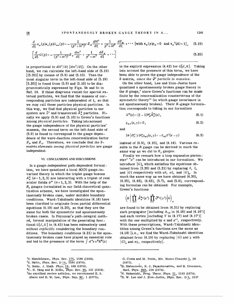
d 1 dM2 1 dZA + - + . o . - % ( P ) t v ( ~ ) G & v ( ~ ) = - (*2 ++iZ)2 'AT * 2 + ~ 2 d S d5

[with €,(p)p, = O and cU2(A)= 11, (5.19)

1 dm2 [-$G ( p ) = - ( p 2 + m 2 ) 2 z Z " ~ i p Z + m Z EL+... dt; 1

is proportional to d1l2/d[ [dwz2/d[]. On the other hand, we can calculate the left-hand s ide of (5.19) [(5.20)] by means of (5.9) and (5.10). Then the most s ingular t e r m i n the left-hand s ide of (5.19) [5.20)] is found f r o m (5.9) and (5.10) to b e d ia - grammatical ly expressed by Figs. 5b and 5c i n Ref. 14. I£ these d iagrams vanish for special ex- t e rna l par t ic les , we find that the m a s s e s of c o r - responding par t i c les a r e independent of 6, s o that we may cal l these par t i c les physical par t ic les . In th i s way, we find that physical par t i c les in our sys tem a r e G3 and t ransversa l 2; part ic les . F i - nally we apply (5.9) and (5.10) to Green's functions among physical par t i c les . Taking into account the gauge independence of the physical par t ic les ' m a s s e s , the second t e r m on the left-hand s ide of (5.9) i s found to correspond t o the gauge dependence of the wave-function renormalization factor ZA and 2 , . Therefore, we conclude that the S- matr ix elements anlong physical par t i c les a r e gauge independent.

VI. CONCLUSIONS AND DISCUSSIONS

In a gauge-independent path-dependent fo rmal - i sm, we have quantized a local SO(3) gauge-in- var iant theory in which the t r iplet gauge bosons A: ( a = 1, 2,3) a r e interacting with a t r iplet of r e a l s c a l a r fields +a (a = 1, 2,3). With the help of the R, gauges formulated in our field-theoretical quantization scheme, we have investigated the spontaneously broken case, under suitable boundary conditions. Ward-Takahashi identities (4.18) have been clarified to originate f r o m par t i a l differential equations (4.19) and (4.20), s o that they a r e the s a m e for both the symmetr ic and spontaneously broken cases . In Feynman's path-integral method, fo rmal manipulation of the generating functional G[J, K ] in (4.43) h a s been extensively used without explicitly considering the boundary conditions. The boundary conditions (4.21) in the spontaneously broken c a s e have played an essent ial role and led to the p resence of the t e r m d 4 z v 6 p ( z )

I

i n the explicit expression (4.42) fo r G[J, K]. Taking into account the p resence of th i s t e r m , we have been able to prove the gauge independence of the S matr ix, s ince the (P3 par t ic le is ~?zassive.

On the other hand, L e e and Zinn-Justin have quantized a spontaneously broken gauge theory in the R gauge,8 s ince Green's functions can be made finite by the renormalizat ion counte r te rms of the symmetr ic theory1= (in which gauge invariance is not spontaneously broken). The i r R-gauge formula- tion corresponds to taking in our fo rmal i sm

and

instead of (4.9), (4.10), and (4.14). Various r e - su l t s in the R gauge can be derived in much the s a m e way a s we did in R! gauges.

Finally we r e m a r k how a loop expansion p a r a m - e te r5 "a" can be introduced in our formalism. We introduce IG), which sa t i s f ies the equations obtained f r o m (3.20) and (3.21) by replacing 8, <, and IG) respectively with a@, a t , and IG),. In much the s a m e way a s we have obtained (4.30), (4.35), (4.42), (4.43), (5.7), and (5.8), corresponding formulas can be obtained: F o r example, Green 's functions

a r e found to b e obtained f r o m (4.31) by replacing each propagator [including A Y c in (4.16) and (4.16')] and each ver tex [including V in (4.17) and (4.17')] with the one multiplied by a and a-', respectively. With these prescr ipt ions, Ward-Takahashi iden- t i t i es among Green ' s functions a r e the s a m e as (4.18) [i.e., we find the Ward-Takahashi identities obtained f r o m (4.18) b y replacing IG) and x with IG), and ax, respectively].

's. Mandelstam, Phys. Rev. 175, 1580 (1968). G. Costa and M. Tonin, Riv. Nuovo Cimento 5, 29 2 ~ . Naito, Phys. Rev. D 5, 3584 (1976). (1975). . 3 ~ . Naito, J. Math. Phys. 2, 568 (1978). 6 ~ . Matsumoto, N. J. Papastamatiou, and H. Umezawa, 4 ~ . N. Yang and R . Mills, Phys. Rev. 96, 1 9 1 (1954). Nucl. Phys. E, 236 (1974). 5 ~ s excellent review articles, we recommend E. S. IN. Nakanishi, Prog. Theor. Phys. 51, 1183 (1974).

Abers and B. W. Lee, Phys. Rep. E, 1 (1973); 'B. W. Lee and J. Zinn-Justin, Phys. Rev. D?, 3137

1242 S E I C H I N A I T O A N D S E I Z I A K A H O R I 18 -

(1972). Phys. Rev. 155, 1554 (1967). '1. Bialynicki-Birula, Bull. Acad. Polon. Sci. 11, 135 13R. E . Peierls, Proc. R. Soc. London m, 143 (1952).

(1963). 14G. 't Hooft and M. Veltman, Nucl. Phys. g, 318 'OG. 't Hooft, Nucl. Phys. m, 167 (1971). (1972). "K. Fujikawa, B. W. Lee, and A . I. Sanda, Phys. Rev. 1 5 ~ . W. Lee and J. Zinn-Justin. Phys. Rev. D 5 , 3121

D?, 2923 (1972). (1972). 12p. Higgs, Phys. Lett. 12, 132 (1966); T. W. B. Kibble,

spontaneously broken gauge theory in a gauge-independent path-dependent formalism

Documents