spo2frag v1.0: software for pushover-based...

ECCOMAS Congress 2016 VII European Congress on Computational Methods in Applied Sciences and Engineering

M. Papadrakakis, V. Papadopoulos, G. Stefanou, V. Plevris (eds.) Crete Island, Greece, 5–10 June 2016

SPO2FRAG V1.0: SOFTWARE FOR PUSHOVER-BASED DERIVATION OF SEISMIC FRAGILITY CURVES

Iunio Iervolino1, Georgios Baltzopoulos2, Dimitrios Vamvatsikos3 and Roberto Baraschino4

1 Università degli Studi di Napoli Federico II

Via Claudio 21, 80125 Naples, Italy [email protected]

2 Istituto per le Tecnologie della Costruzione ITC-CNR, URT Napoli c/o DiSt

Via Claudio 21, 80125 Naples, Italy [email protected]

3 National Technical University of Athens

9 Heroon Politechneiou, 157 80 Athens, Greece [email protected]

4 AMRA s.c.a r.l.

Via Nuova Agnano 11, 80125 Naples, Italy [email protected]

Keywords: vulnerability, incremental dynamic analysis, seismic risk, loss assessment.

Abstract. This article presents SPO2FRAG V1.0, the first (beta) version of the Static PushOver to FRAGility software. The SPO2FRAG software is an interactive and user-friendly tool that can be used for approximate, computer-aided calculation of building seismic fragility functions, based on static pushover analysis. It is coded in MATLAB® environment and is currently under development at the Department of Structures for Engineering and Architecture of the University of Naples Federico II. At the core of the SPO2FRAG tool lies the SPO2IDA algorithm, which permits analytical predictions for incremental dynamic analysis summary fractiles at the sin-gle-degree-of-freedom system level. By effectively interfacing SPO2IDA with a series of oper-ations, intended to link the results of static pushover analysis with the variability that typically characterizes non-linear dynamic structural response, SPO2FRAG provides an expedient so-lution to the computationally demanding task of analytically evaluating seismic building fra-gility, which would otherwise require a large number of non-linear dynamic analyses.

Iunio Iervolino, Georgios Baltzopoulos, Dimitrios Vamvatsikos and Roberto Baraschino

1 INTRODUCTION

Seismic risk and loss estimation studies performed within a probabilistic framework employ structural fragility (or vulnerability) functions, which provide the probability of exceeding some predefined performance limit state in a single seismic event, given a certain level of seismic intensity. In the case of structure-specific studies, the trend is to rely increasingly on analytical derivation for these fragility functions. State-of-the-art in analytical fragility estimation is the use of non-linear dynamic analyses – for example, incremental dynamic analysis (IDA, [1]), the cloud method [2] or multi-stripe analysis [3]. However, despite the advantages of the ana-lytical approaches over the damage probability matrices and empirical fragility curves em-ployed earlier, their chief disadvantage remains the computational burden involved [4], which may include the selection and manipulation of hazard-consistent ground motion records.1

In order to sidestep the computationally demanding methods of seismic structural assessment that involve non-linear dynamic analysis, engineers have long relied on approximate methods, such as static non-linear procedures, which estimate seismic demand of the structure by making recourse to an equivalent single-degree-of-freedom (SDOF) oscillator [6]. A simple and effec-tive link between IDA and static non-linear analysis has been provided by the SPO2IDA algo-rithm [7], which acts as a predictive equation of the fractile IDA curves for SDOF systems with multi-linear pushover curves. The SPO2IDA algorithm forms the backbone around which the SPO2FRAG (Static Pushover to Fragility) tool, a MATLAB® coded software whose presenta-tion is the objective of the present paper, is built. SPO2FRAG offers an expedient solution to the analytical derivation of seismic fragility for buildings and can provide support to previously developed seismic risk assessment software such as the one described in [8].

The remainder of this article is structured in the following manner: first a brief presentation of past research most relevant to the development of the SPO2FRAG tool is provided. This is followed by an operational description of the software itself, complete with a flowchart and graphical user interface (GUI) description. Subsequently, an example application is provided, accompanied by a comparison of the SPO2FRAG output with a set of fragility functions de-rived by means of IDA. Finally, some commentary and discussion on development concludes the article.

2 BACKGROUND

2.1 Static pushover to IDA

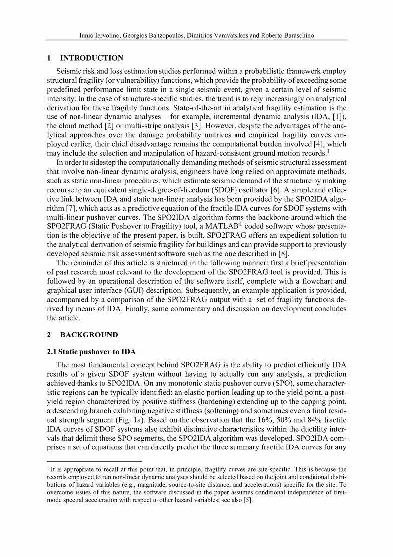
The most fundamental concept behind SPO2FRAG is the ability to predict efficiently IDA results of a given SDOF system without having to actually run any analysis, a prediction achieved thanks to SPO2IDA. On any monotonic static pushover curve (SPO), some character-istic regions can be typically identified: an elastic portion leading up to the yield point, a post-yield region characterized by positive stiffness (hardening) extending up to the capping point, a descending branch exhibiting negative stiffness (softening) and sometimes even a final resid-ual strength segment (Fig. 1a). Based on the observation that the 16%, 50% and 84% fractile IDA curves of SDOF systems also exhibit distinctive characteristics within the ductility inter-vals that delimit these SPO segments, the SPO2IDA algorithm was developed. SPO2IDA com-prises a set of equations that can directly predict the three summary fractile IDA curves for any

1 It is appropriate to recall at this point that, in principle, fragility curves are site-specific. This is because the records employed to run non-linear dynamic analyses should be selected based on the joint and conditional distri-butions of hazard variables (e.g., magnitude, source-to-site distance, and accelerations) specific for the site. To overcome issues of this nature, the software discussed in the paper assumes conditional independence of first-mode spectral acceleration with respect to other hazard variables; see also [5].


SDOF system, with a given quadrilinear backbone geometry; this introduces an approximation but has the advantage of eschewing the need for laborious computations. An example of SPO2IDA-predicted fractile IDA curves is given in Fig. 1b, where the predictions are compared against the corresponding fractiles of explicitly calculated IDAs.

Figure 1: (a) Generic SDOF oscillator’s quadri-linear backbone curve plotted in reduction factor (R, ratio of

maximum to yield force) – ductility (μ, ratio of maximum to yield displacement) coordinates and (b) an example of SPO2IDA-predicted 16%, 50%, 84% fractile IDA curves, super-imposed over the fractile and individual IDAs

calculated analytically for the same SDOF system using the FEMA P695 [9] far-field set of forty-four records. Backbone geometry is defined by the parameters αh (post-yield to elastic stiffness ratio), μc (ductility at capping point marking the beginning of the descending branch), ac (post-capping to elastic stiffness ratio) and μf (fracture

ductility.)

2.2 Multi-linear fit of the monotonic backbone curve

Another important part of the SPO2FRAG algorithm is the automatization of obtaining a multi-linear backbone for the equivalent SDOF oscillator. As recently as – roughly – a decade ago, the norm for the implementation of static non-linear procedures (e.g., [10]) used to be a combination of simple elastic-perfectly-plastic or bi-linear hardening approximations of SPO backbones coupled with R-μ-T relationships (e.g., [11]) that only consider some central value of inelastic response. Under these circumstances, empirical “rules of thumb” for the multi-linear fit chosen for the SPO may have been good enough, but this may no longer be the case.

Advances in computing power and the sophistication of numerical modelling, for the non-linear aspects of structural behavior, have gradually led to SPO curves containing appreciable initial curvature (in cases where cracking is a factor) and descending post-peak-strength branches. In order to exploit the capabilities of more powerful R-μ-T relationships, such as SPO2IDA, there is a need for an efficient fully quadrilinear fitting scheme of such elaborate SPO backbones. A set of rules to that effect was proposed in [12], based on a study that em-ployed IDA of SDOF systems with curvilinear and piece-wise-linear backbones.

2.3 SDOF to MDOF conversion of the fractile IDA curves

SPO2IDA can provide (an estimate of) the 16%, 50% and 84% fractile IDA curves of an equivalent SDOF system, processing a piecewise-linear backbone curve derived from the SPO of a given structure. The SDOF IDAs naturally come in reduction factor-ductility terms and therefore, in order to relate these IDA curves back to the original MDOF system, a series of

10

1yiel

dR

FF

�

yield� � � �

maxR

0c�

f�

h�

c�

pr

RS

aS

a�

max yield� � � �

Individual IDA curves

IDA fractiles

SPO2IDA fractiles

Multi-linear backbone

(b)

(a)

yiel

d

0 5 10 150

2

4

6

8

10

12


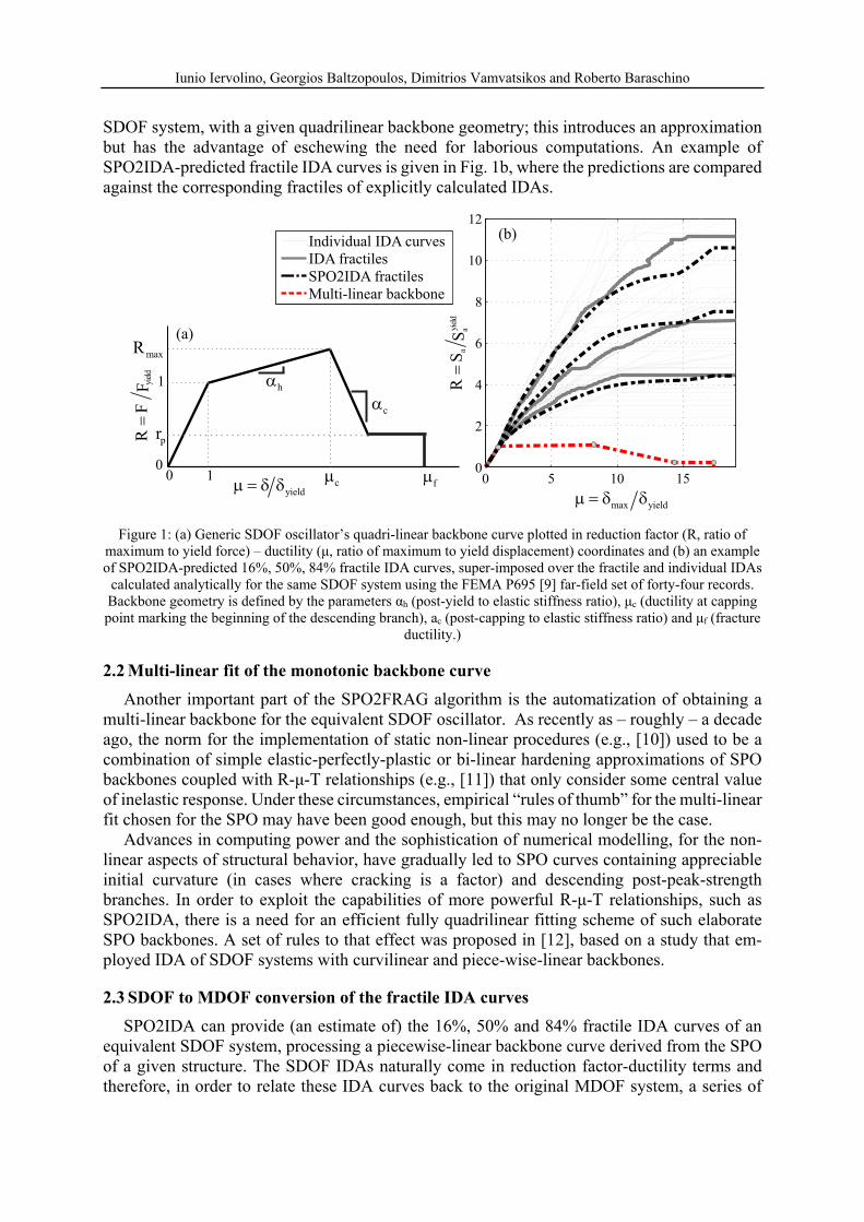
conversion operations are necessary (see Fig. 2). These conversions entail passage from non-dimensional coordinates R - μ to spectral acceleration – roof drift format, the possibility of adding the response variability at the nominal yield point that the MDOF system experiences due to the effect of higher modes (but is lost on its SDOF counterpart, [13]) and possibly a roof drift to inter-storey drift conversion, since the latter is oftentimes better suited for the definition of limit-state thresholds.

2.4 IM-based parametric fragility functions

The final output and stated objective of SPO2FRAG is the estimation of fragility functions for building-type structures. A fragility function provides the conditional probability that a structure will exceed a limit-state threshold (“fail”) in a single seismic event, given a certain ground motion intensity measure (IM) level. If it is assumed that the level of seismic intensity causing failure (or, equivalently, the capacity of the structure per limit-state in IM terms,

C,LSIM ) is a random variable that follows some specific model, for example the log-normal

distribution, determining the fragility function boils down to estimating the mean-of-the-loga-rithm of capacity per limit-state, , and the logarithmic standard deviation, . This can be

seen in Eq. 1, where denotes the Gauss function.

,

ln

C LS

imP IM im

(1)

When the median and 16%, 84% fractile IDA curves are provided for the structure, one may estimate these two parameters by adopting a threshold engineering demand parameter (EDP) value (or probability distribution thereof) for each limit state – see for example Fig. 2c.

Figure 2: (a) Example of SPO2IDA-predicted 16%, 50% and 84% fractile SDOF IDA curves in terms of reduc-tion factor – ductility, (b)conversion to first mode spectral acceleration – inter-storey drift ratio, (c) estimation of fragility function parameters assuming a log-normal distribution for the seismic intensity level causing exceed-

ance of each limit-state threshold, C,LSIM .

log(I

M)

log(EDP)

ProbabilisticLimit-statethreshold

medianIDA curve

16% fractileIDA curve


0 2 4 6 8 100

1

2

3

4

5

6

7

8

0 1 2 30

0.2

0.4

0.6

0.8

1

1.2

Sa(T

1, 5%

) (g

)

θmax

(%)

yie

ld

aa

RS

S�

max yieldu u� �

SPO-basedmulti-linear backbone

SPO2IDASDoF IDA fractile curves

IM - EDP formatapproximated IDA fractile curves

col,84%R

col,50%R

col,16%Rmedian

IDA curve



� �1a col,84%S T

� �1a col,16%S T

� �1a col,50%S T � �C,LS 84%

log IM

� �C,LS 16%log IM

(a) (b) (c)


2.5 Model uncertainty in seismic structural response

SPO2FRAG simulates non-linear dynamic analysis via the SPO2IDA algorithm. Actual IDA, using a deterministic numerical model of the structure, can provide an estimate of record-to-record (aleatory) variability characterizing structural response. However, modelling parameters (such as material properties, member geometry, mass distribution, etc.) may also exhibit their own uncertainty, which will necessarily affect the distribution of C,LSIM . Furthermore, some

specific cases may violate some of the assumptions behind IDA to a certain extent, which can also result in additional uncertainty infiltrating the results. One, very simple, approach towards accounting for this additional uncertainty is to consider that the mean logarithmic capacity is itself a random variable, assumed, for example, normally distributed with a standard devia-tion U (e.g., [14]). This additional parameter can be either obtained directly from relevant stud-

ies in the literature or estimated still via SPO2IDA [15].

3 SPO2FRAG, OPERATIONAL OUTLINE

3.1 Graphical user interface and flowchart

The SPO2FRAG software revolves around a GUI that allows the user prompt visualization of all intermediate results produced by the various modules and sub-routines. The individual modules that comprise the operational part of the software are the input interfaces, automatic multi-linearization module, dynamic characteristics toolbox, SPO2IDA module, interfaces for definition of limit states, their corresponding thresholds and any additional sources of uncer-tainty, the fragility function module and the output post-processing module. A flowchart of SPO2FRAG’s operation is presented in Fig. 3 and a more detailed description of the same is given in the following paragraphs.

3.2 Data input, pre-processing and multi-linear fit

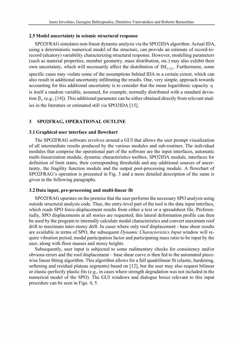
SPO2FRAG operates on the premise that the user performs the necessary SPO analysis using outside structural analysis code. Thus, the entry-level part of the tool is the data input interface, which reads SPO force-displacement results from either a text or a spreadsheet file. Preferen-tially, SPO displacements at all stories are requested; this lateral deformation profile can then be used by the program to internally calculate modal characteristics and convert maximum roof drift to maximum inter-storey drift. In cases where only roof displacement - base shear results are available in terms of SPO, the subsequent Dynamic Characteristics Input window will re-quire vibration period, modal participation factor and participating mass ratio to be input by the user, along with floor masses and storey heights.

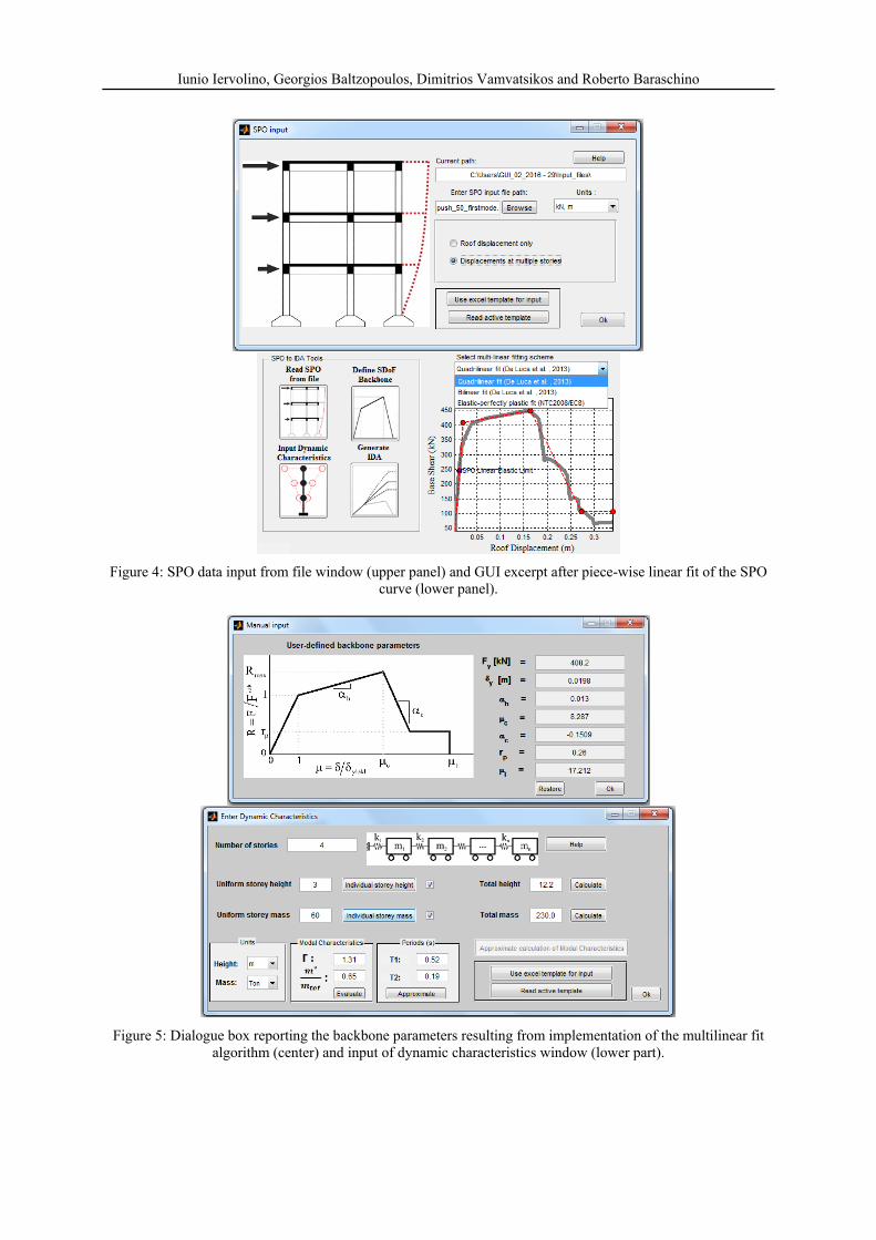
Subsequently, user input is subjected to some rudimentary checks for consistency and/or obvious errors and the roof displacement – base shear curve is then fed to the automated piece-wise linear fitting algorithm. This algorithm allows for a full quadrilinear fit (elastic, hardening, softening and residual plateau segments) based on [12], but the user may also request bilinear or elastic-perfectly plastic fits (e.g., in cases where strength degradation was not included in the numerical model of the SPO). The GUI windows and dialogue boxes relevant to this input procedure can be seen in Figs. 4, 5.


Figure 3: SPO2FRAG V1.0 flowchart.

Input SPO results

Start

Piece-wise linearfit of SPO curve

SPOdisplacements

availableat all floors?

NO, roof-level only

YES

Input massesand floor heights

Input masses,foor heightsand dynamic

characteristics

Calculatedynamic

characteristics

Run SPO2IDAand generateIDA fractiles

Select SPOfitting scheme

Convert IDAfractiles to

MDOF IM, EDP

Estimateand add

variabilityat yield due

to highermodes

Accountfor model

uncertainty?

YES

NO

Directassignment

or MC?

MC

Assign U�

Define distributionof uncertain SDOFmodel parameters(F , )yield μ α αcap h c, , , rp

RunMonte Carlosimulation

Update IDAs

Define limit statesand their EDP

thresholds

Deterministiclimit state

thresholds?

YES

NO

Perform MCsamplingthreshold

distribution

Calculatefragilityfunction

parameters

End

- Quadrilinear- Bilinear- Elastoplastic


Figure 4: SPO data input from file window (upper panel) and GUI excerpt after piece-wise linear fit of the SPO

curve (lower panel).

Figure 5: Dialogue box reporting the backbone parameters resulting from implementation of the multilinear fit algorithm (center) and input of dynamic characteristics window (lower part).


3.3 SPO2IDA and SDOF to MDOF conversions

Once data input is completed and a multi-linear fit of the SPO curve has been obtained, the SPO2IDA algorithm is launched, providing the 16%, 50% and 84% fractile SDOF IDA curve predictions in R-μ terms. The SPO2IDA output is automatically converted into spectral accel-eration – drift format, using the dynamic characteristics of the structure. In cases where the SPO displacements at all storeys have been provided, the IDAs are converted in maximum intersto-rey drift ratio (IDR) terms by default; otherwise, EDP is set to roof drift. Even in the latter case, the user may still choose to convert to IDR, by selecting an appropriate approximation for the lateral post-yield deformation profile.

After this operation, an issue pertaining to the MDOF IDA curves that remains to be ad-dressed is the fact that the MDOF system should exhibit greater record-to-record variability than its equivalent SDOF, due to the effect of higher modes of vibration. This additional varia-bility is estimated by means of in-built empirical rules, injected at the nominal yield point and propagated along the IDA 16% and 84% fractiles.

Figure 6. GUI excerpt showing the approximate (predicted) fractile IDA curves after completion of SDOF to

MDOF conversion (upper panel) and window for the definition of limit states and limit-state-thresholds in terms of EDP (lower panel).

3.4 Limit-states and handling additional uncertainty

By default, the SPO2FRAG tool recognizes four limit states: fully operational, immediate occupancy, life safety and collapse prevention (see [16] for definitions). In cases where the SPO exhibits a negative-stiffness, softening branch a fifth limit state, dynamic instability will appear, corresponding to the IDA flat-lines. The user may also define more limit states via the GUI. In all cases, the user must define thresholds in terms of EDP, which determine exceedance of each limit state. Such thresholds need not be deterministic; the user has the option to treat them in a


probabilistic manner, by assuming that some thresholds follow a lognormal distribution, whereas the median and log-standard deviation of said distribution must be defined (Fig. 6).2

In cases where the user wishes to include (additional) modelling uncertainty into the calcu-lation, two alternative options are available in the relevant GUI panel. First option is to define a logarithmic standard deviation U for mean logarithmic capacity at one of the predefined

limit states. This additional uncertainty is then propagated along the IDA curves. The second option is to consider some of the parameters that define the SDOF multi-linear backbone curve as random variables. In this second case, it is possible for the user to define the variance of the backbone parameters one wishes to treat probabilistically (log-normal distribution is assumed where the median is by default taken as the value initially provided by the automated fitting algorithm). Subsequently, Monte Carlo simulation is performed internally, where SPO2IDA realizations are created by sampling from within the user-defined parameter distributions and the IDA fractiles are updated accordingly.

3.5 Estimation of fragility curve parameters

Once the series of operations described above have been concluded, the fragility function parameters per limit state can be estimated based on the resulting approximated IDA curves of the structure. In the case of deterministic definition for the limit state EDP thresholds the loga-rithmic mean is taken simply as the logarithm of the median IDA value at each threshold EDP level. The standard deviation can be estimated as either the distance (in log-space) be-tween the median and 84% fractile IDA or half the distance between the 16% and 84% fractile IDAs, at the discretion of the user (the latter being the default option, Eq. 2).

50%,

50% 16%, ,

84% 16%, ,

ln

ln , or alternatively

1 2 ln

C LS

C LS C LS

C LS C LS

IM

IM IM

IM IM

(2)

In cases where the user has defined a probability distribution for the EDP threshold, rather than a deterministic value thereof, the parameter estimation procedure remains conceptually the same. The difference lies in the fact that Eq. 2 is applied for a number of EDP threshold reali-zations per limit state, sampled from the user-defined distribution and the final parameter esti-mates are provided by Monte Carlo simulation.

4 EXAMPLE APPLICATION

4.1 Four-storey “modern code” RC frame

In order to provide a fully-worked example of SPO2FRAG usage, a four-storey, bare, rein-forced concrete (RC), plane frame was employed. This frame belongs to a symmetrical building designed under EN 1998-1 provisions in the context of a previous study (see [17] for more details) and was modelled numerically using the OpenSees open-code, structural analysis soft-ware [18]. Overall dimensions, member cross-sections, floor masses, shapes and periods of the first and second vibration modes and the SPO curve resulting from a first-mode-proportional

2 Note that, for the sake of consistency limit state ranking (from milder to more severe) is adjusted automatically by the software, based on the corresponding user-defined (median or deterministic) thresholds.


lateral load profile are reported in Fig. 7. Inelasticity in the RC members was modelled follow-ing the concentrated plasticity approach, with plastic hinges at members’ ends represented by rotational springs featuring trilinear backbones and hysteresis loops exhibiting mild pinching [19]. Concrete cracking was accounted for via the smeared crack approach of reducing the elas-tic pre-cracking stiffness of each member according to axial load [20].

Figure 7: Dimensions, member cross-sections, floor masses, first two modes of natural vibration and first-mode

SPO curve of the code-conforming four-storey RC frame used in the SPO2FRAG example application.

4.2 Example – fragility function calculation through SPO2FRAG

The SPO curve of the four-storey RC frame presented in the preceding paragraph is used as input for SPO2FRAG; displacements at all four diaphragms are provided via the input interface.

Figure 8: GUI view after implementation of the SPO2FRAG tool for an eight-storey “high-code” bare RC frame.

360

@to

n

ton50

40

40

x

32.

m

3@ 5.00 m

33

@ 0. m

6 /30 0

T1 = . s0 52 T2= s0.19

45

45

x

40

40

x

45

45

x

35

35

x

40

40

x

40

40

x

35

35

x

35

35

x

35

35

x

6 /30 06 /30 0

6 /30 0 6 /30 06 /30 0

plastic hinge locations

0.10 0.20 0.30

100

200

300

400

Roof Displacement (m)

Bas

e S

hea

r (k

N)

SPO curve

Multi-linear fit

αh=1.4%

αc =

-14.4%

rp= 21.8%


The roof displacement – base shear SPO is then subjected to a multilinear fit by the algorithm based on [12] (resulting fit is visible in Figs. 7, 8 and the corresponding backbone parameters in Fig. 4). Due to the availability of SPO results at all storeys, the only further input required, prior to obtaining the SPO2IDA approximate IDA fractiles, are the storey heights and masses (vibration period, modal participation factor and participating mass ratio are all calculated in-ternally).

For this particular example, deterministic EDP thresholds (in terms of IDR) were assumed for the calculation. Indicative IDR thresholds for each limit state were calculated based on the acceptance criteria plastic rotation values for RC members found in [16]. A snapshot of the GUI display at the conclusion of this SPO2FRAG run can be seen in Fig. 8.

5 SPO2FRAG VS. IDA

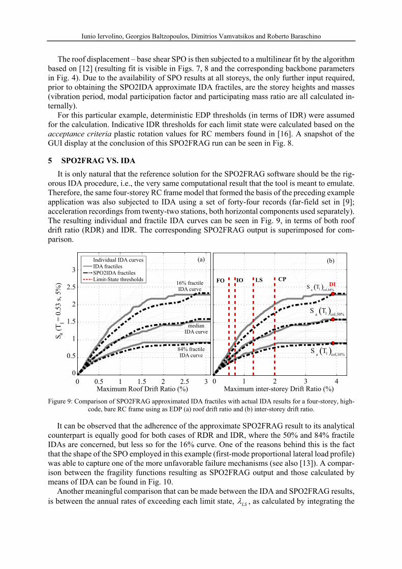
It is only natural that the reference solution for the SPO2FRAG software should be the rig-orous IDA procedure, i.e., the very same computational result that the tool is meant to emulate. Therefore, the same four-storey RC frame model that formed the basis of the preceding example application was also subjected to IDA using a set of forty-four records (far-field set in [9]; acceleration recordings from twenty-two stations, both horizontal components used separately). The resulting individual and fractile IDA curves can be seen in Fig. 9, in terms of both roof drift ratio (RDR) and IDR. The corresponding SPO2FRAG output is superimposed for com-parison.

Figure 9: Comparison of SPO2FRAG approximated IDA fractiles with actual IDA results for a four-storey, high-

code, bare RC frame using as EDP (a) roof drift ratio and (b) inter-storey drift ratio.

It can be observed that the adherence of the approximate SPO2FRAG result to its analytical counterpart is equally good for both cases of RDR and IDR, where the 50% and 84% fractile IDAs are concerned, but less so for the 16% curve. One of the reasons behind this is the fact that the shape of the SPO employed in this example (first-mode proportional lateral load profile) was able to capture one of the more unfavorable failure mechanisms (see also [13]). A compar-ison between the fragility functions resulting as SPO2FRAG output and those calculated by means of IDA can be found in Fig. 10.

Another meaningful comparison that can be made between the IDA and SPO2FRAG results, is between the annual rates of exceeding each limit state, LS , as calculated by integrating the

(a) (b)

0 1 2 3 4Maximum inter-storey Drift Ratio (%)

DIIO LS CPFO

0 0.5 1 1.5 2 2.5 3

0

0.5

1

1.5

2

2.5

3

Maximum Roof Drift Ratio (%)

Sa

(T1=

0.5

3 s

, 5%

)

Individual IDA curves

IDA fractiles

SPO2IDA fractiles

Limit-State thresholds

� �1a col,16%S T

� �1a col,50%S T

� �1a col,84%S T

medianIDA curve




fragility functions from the two procedures with the hazard curve for a given site, according to Eq. 3.

, LS C LS im

IM

P IM im d (3)

In Eq. 3 the notation im is used to signify the rate of exceeding a given IM value while for the

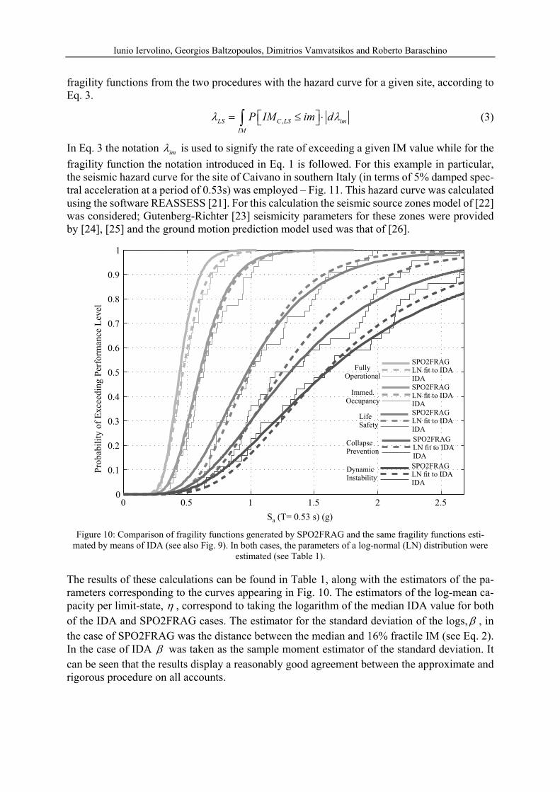
fragility function the notation introduced in Eq. 1 is followed. For this example in particular, the seismic hazard curve for the site of Caivano in southern Italy (in terms of 5% damped spec-tral acceleration at a period of 0.53s) was employed – Fig. 11. This hazard curve was calculated using the software REASSESS [21]. For this calculation the seismic source zones model of [22] was considered; Gutenberg-Richter [23] seismicity parameters for these zones were provided by [24], [25] and the ground motion prediction model used was that of [26].

Figure 10: Comparison of fragility functions generated by SPO2FRAG and the same fragility functions esti-

mated by means of IDA (see also Fig. 9). In both cases, the parameters of a log-normal (LN) distribution were estimated (see Table 1).

The results of these calculations can be found in Table 1, along with the estimators of the pa-rameters corresponding to the curves appearing in Fig. 10. The estimators of the log-mean ca-pacity per limit-state, , correspond to taking the logarithm of the median IDA value for both of the IDA and SPO2FRAG cases. The estimator for the standard deviation of the logs, , in the case of SPO2FRAG was the distance between the median and 16% fractile IM (see Eq. 2). In the case of IDA was taken as the sample moment estimator of the standard deviation. It can be seen that the results display a reasonably good agreement between the approximate and rigorous procedure on all accounts.

0 0.5 1 1.5 2 2.50

0.1

0.2

0.3

0.4

0.5

0.6

0.7

0.8

0.9

1

Pro

bab

ilit

y o

f E

xce

edin

g P

erfo

rman

ce L

evel

FullyOperational

Immed.Occupancy

LifeSafety

CollapsePrevention

DynamicInstability

SPO2FRAGLN fit to IDAIDA





S (T= 0.53 s) (g)a


Figure 11: Hazard curve for an Italian site: annual rate of exceedance of 5% damped spectral acceleration at a period of 0.53s (period of equivalent SDOF of the four-storey frame in the example application).

Limit state exp

(IDA) exp

(SPO2FRAG)

(IDA)

(SPO2FRAG)

LS (IDA)

LS (SPO2FRAG)

Fully Operational

0.456 g 0.442 g 0.294 0.187 44.9 10 44.5 10

Immediate Occupancy

0.631 g 0.599 g 0.318 0.269 42.0 10 42.1 10

Life Safety 0.988 g 0.972 g 0.362 0.401 55.3 10 56.6 10

Collapse Prevention

1.260 g 1.308 g 0.410 0.484 52.8 10 53.5 10

Global Dynamic Instability

1.590 g 1.584 g 0.571 0.534 51.7 10 52.4 10

Table 1: Parameter estimators for the log-normal fragility functions of the illustrative example (see also Fig. 10) and corresponding calculated annual rates of exceeding each limit state at a site in Southern Italy.

6 CONCLUSIONS

This article dealt with the introduction of the SPO2FRAG V1.0 software. It is an interactive tool, coded in MATLAB® , that can be used for approximate, computer-aided calculation of building seismic fragility functions, based on static pushover analysis. It was shown that SPO2FRAG can provide a convenient and expeditious solution to the problem of analytical calculation of building fragility functions, at least in cases where the basic assumptions behind SPO analysis and IDA hold.

In a future, second version of the SPO2FRAG tool, whose development is currently under-way, additional options are expected to be available. These additional features will include, among others the possibility to manage input consisting of more than one SPO curve per struc-ture (corresponding to either loads applied in two principal directions of a three-dimensional structure, or different load patterns applied in the same direction – or both) and an in-built library of deformation limits per limit state from the literature.

10-1

100

10-8

10-6

10-4

10-2

100

Sa(T=0.53s) (g)

λim


ACKNOWLEDGEMENTS

The work presented in this paper was developed within the AXA-DiSt (Dipartimento di Strutture per l’Ingegneria e l’Architettura, Università degli Studi di Napoli Federico II) 2014-2017 research program, funded by AXA-Matrix Risk Consultants, Milan, Italy. The second author also wishes to acknowledge the support of the European Research Executive Agency via Marie Curie grant PCIG09-GA-2011-293855.

REFERENCES

[1] D. Vamvatsikos, C.A. Cornell. Incremental dynamic analysis. Earthquake Engineering and Structural Dynamics, 31, 491-514, 2002.

[2] P. Bazzuro, C.A. Cornell, N. Shome, J.E. Carballo. Three proposals for characterizing MDOF non-linear seismic response. Journal of Structural Engineering, 124, 1281-1289, 1998.

[3] N. Shome, C.A. Cornell, P. Bazzuro, J.E. Carballo. Earthquakes, records and non-linear responses. Earthquake Spectra, 14(3), 469-500, 1998.

[4] G.M. Calvi,R. Pinho, G. Magenes, J.J. Bommer, L.F. Restrepo-Vélez, H. Crowley. De-velopment of seismic vulnerability assessment methodologies over the past 30 years. ISET Journal of Earthquake Technology, 43(3), 75-104, 2006.

[5] N. Luco, C.A. Cornell. Structure-Specific Scalar Intensity Measures for Near-Source and Ordinary Earthquake Ground Motions. Earthquake Spectra, 23(2), 357-392, 2007.

[6] M. Fragiadakis, D. Vamvatsikos, M. Ascheim. Application of nonlinear static procedures for seismic assessment of regular RC moment frame buildings. Earthquake Spectra, 30(2), 767–794, 2014.

[7] D. Vamvatsikos, C.A. Cornell. Direct estimation of the seismic demand and capacity of oscillators with multi-linear static pushovers through IDA. Earthquake Engineering and Structural Dynamics, 35, 1097–1117, 2006.

[8] F. Petruzzelli, I. Iervolino. FRAME V.1.0: A rapid fragility-based seismic risk assessment tool. Proceedings of the Second European Conference on Earthquake Engineering and Seismology, 2ECEES, Istanbul, Turkey, 24-29 August, 2014.

[9] FEMA P695. Quantification of Building Seismic Performance Factors. Federal Emer-gency Management Agency, Washington D.C., 2009.

[10] P. Fajfar. A nonlinear analysis method for performance based seismic design. Earthquake Spectra, 16(3), 573-592, 2000.

[11] T. Vidic, P. Fajfar, M. Fischinger. Consistent inelastic design spectra: strength and dis-placement. Earthquake Engineering and Structural Dynamics, 23, 507-521, 1994.

[12] F. De Luca, D. Vamvatsikos, I. Iervolino. Near-optimal piecewise linear fits of static pushover capacity curves for equivalent SDOF analysis. Earthquake Engineering and Structural Dynamics, 42(4), 523-543, 2013.

[13] D. Vamvatsikos, C.A. Cornell. Direct estimation of seismic demand and capacity of mul-tiple-degree-of-freedom systems through incremental dynamic analysis of single degree of freedom approximation. Journal of Structural Engineering, 131, 589-599, 2005.


[14] C.A. Cornell, F. Jalayer, R.O. Hamburger, D.A. Foutch. The probabilistic basis for the SAC/FEMA steel moment frame guidelines. Journal of Structural Engineering, 128, 526-533, 2002.

[15] M. Fragiadakis, D. Vamvatsikos. Fast performance uncertainty estimation via pushover and approximate IDA. Earthquake Engineering and Structural Dynamics, 39(6), 683-703, 2010.

[16] FEMA 356. Prestandard and commentary for the seismic rehabilitation of buildings. Federal Emergency Management Agency, Washington D.C., 2000.

[17] G. Baltzopoulos, E. Chioccarelli, I. Iervolino. The displacement coefficient method in near-source conditions. Earthquake Engineering and Structural Dynamics, 44(7), 1015-1033, 2015.

[18] F. McKenna, G.L. Fenves, M.H. Scott, B. Jeremic. Open System for Earthquake Engi-neering Simulation (OpenSees). Pacific Earthquake Engineering Research Center, Uni-versity of California, Berkeley, CA, 2000.

[19] L.F. Ibarra, R.A. Medina, H. Krawinkler. Hysteretic models that incorporate strength and stiffness deterioration. Earthquake Engineering and Structural Dynamics, 34, 1489-1511, 2005.

[20] T.B. Panagiotakos, M. Fardis. Deformations of Reinforced Concrete Members at Yield-ing and Ultimate. ACI Structural Journal, 98(2), 135-148, 2001.

[21] I. Iervolino, E. Chioccarelli, P. Cito. REASSESS V1.0: A computationally efficient soft-ware for probabilistic seismic hazard analysis. Paper submitted to ECCOMAS Congress 2016: VII European Congress on Computational Methods in Applied Sciences and Engi-neering. M. Papadrakakis, V. Papadopoulos, G. Stefanou, V. Plevris (eds.), Crete Island, Greece, 5–10 June 2016.

[22] C. Meletti, F. Galadini, C. Valensise, M. Stucchi, R. Basili, S. Barba, G. Vannucci, E. Boschi. A seismic source zone model for the seismic hazard assessment of the Italian territory. Tectonophysics, 450, 85-108, 2008.

[23] B. Gutenberg, C.F. Richter. Frequency of earthquakes in California. Bulletin of the Seis-mological Society of America, 34, 185-188, 1944.

[24] S. Barani, D. Spallarossa, P. Bazzurro. Disaggregation of probabilistic ground-motion hazard in Italy. Bulletin of the Seismological Society of America, 99, 2638-2661, 2009.

[25] S. Barani, D. Spallarossa, P. Bazzurro. Erratum to disaggregation of probabilistic ground-motion hazard in Italy. Bulletin of the Seismological Society of America, 100, 3335-3336, 2010.

[26] N.N. Ambraseys, K.A. Simpson, J.J. Bommer. Prediction of horizontal response spectra in Europe. Earthquake Engineering and Structural Dynamics, 25, 371-400, 1996.

spo2frag v1.0: software for pushover-based...

Documents