spmats manual.pdf
DESCRIPTION
spMats ManualTRANSCRIPT

v7.0 This Computer program (including software design, programming structure, graphics, manual, and on-line help) was created and published by STRUCTUREPOINT, formerly the Engineering Software Group of the Portland Cement Association (PCA) for the engineering analysis and design of concrete foundation mats, combined footings, and slabs on grade. While STRUCTUREPOINT has taken every precaution to utilize the existing state-of-the-art and to assure the correctness of the analytical solution techniques used in this program, the responsibilities for modeling the structure, inputting data, applying engineering judgment to evaluate the output, and implementing engineering drawings remain with the structural engineer of record. Accordingly, STRUCTUREPOINT does and must disclaim any and all responsibility for defects or failures of structures in connection with which this program is used.
Neither this manual nor any part of it may be reproduced, edited, transmitted by any means electronic or mechanical or by any information storage and retrieval system, without the written permission of STRUCTUREPOINT, LLC.
All products, corporate names, trademarks, service marks, and trade names referenced in this material are the property of their respective owners and are used only for identification and explanation without intent to infringe. spMats™ is a trademark of STRUCTUREPOINT, LLC.
Copyright © 2002 – 2009, STRUCTUREPOINT, LLC. All Rights Reserved.

Table of Contents
Chapter 1 – Introduction .................................................................................................1-1
Program Features.........................................................................................................1-1 Program Capacity ........................................................................................................1-3 System Requirements ..................................................................................................1-3 Terms...........................................................................................................................1-3 Conventions.................................................................................................................1-4 Installing, Purchasing and Licensing spMats ..............................................................1-4
Chapter 2 – Method of Solution ......................................................................................2-1 The Global Coordinate system ....................................................................................2-1 Mesh Generation .........................................................................................................2-2 Preparing the Input ......................................................................................................2-3 The Plate Element........................................................................................................2-4 Nodal Restraints and Slaved Degrees-of-Freedom......................................................2-5 The Winkler’s Foundation...........................................................................................2-5 Piles .............................................................................................................................2-6 The Nonlinear Solution ...............................................................................................2-7 Types of Loads ............................................................................................................2-7 Load Cases and Combinations ....................................................................................2-9 The Solution ................................................................................................................2-9 Element Internal Moments ........................................................................................2-10 Element Design Moments .........................................................................................2-11 Required Reinforcement............................................................................................2-12 Punching Shear Check...............................................................................................2-14 Program Results ........................................................................................................2-17
Chapter 3 – spMats Interface...........................................................................................3-1 File Menu ....................................................................................................................3-4 Define Menu................................................................................................................3-5 Assign Menu................................................................................................................3-7 Solve Menu..................................................................................................................3-8 View Menu ..................................................................................................................3-8 Options Menu ..............................................................................................................3-9 Help Menu.................................................................................................................3-11
iv
Chapter 4 – Operating spMats......................................................................................... 4-1 Creating a New Data File............................................................................................ 4-1 Opening an Existing Data File .................................................................................... 4-2 Saving the Data ........................................................................................................... 4-2 Reverting to the Last Saved Data File......................................................................... 4-3 Printing Results ........................................................................................................... 4-4 Printing the screen....................................................................................................... 4-6 Exiting the Program .................................................................................................... 4-7 Defining the General Info ........................................................................................... 4-7 Defining the Grid ........................................................................................................ 4-8 Managing Libraries ................................................................................................... 4-12 Defining Material Properties..................................................................................... 4-15 Defining the Restraints.............................................................................................. 4-20 Defining the Loads.................................................................................................... 4-23 Assigning the material properties.............................................................................. 4-26 Assigning the Restraints............................................................................................ 4-31 Applying the Loads................................................................................................... 4-34 Solving the Model..................................................................................................... 4-36 Viewing the Results .................................................................................................. 4-38 Viewing the Contours ............................................................................................... 4-40 Accessing the 3D View............................................................................................. 4-41 Defining the Options................................................................................................. 4-43
Chapter 5 – Examples ..................................................................................................... 5-1 Example 1 ................................................................................................................... 5-1 Example 2 ................................................................................................................. 5-10
Appendix........................................................................................................................ A-1 Conversion Factors - English to SI ............................................................................ A-1 Conversion Factors - SI to English. ........................................................................... A-1 Contact Information ................................................................................................... A-2

License Agreements
STRUCTUREPOINT EVALUATION SOFTWARE LICENSE AGREEMENT BY CLICKING THE “I AGREE” ICON BELOW, OR BY INSTALLING, COPYING, OR OTHERWISE USING THE SOFTWARE OR USER DOCUMENTATION, YOU AGREE TO BE BOUND BY THE TERMS OF THIS AGREEMENT, INCLUDING, BUT NOT LIMITED TO, THE WARRANTY DISCLAIMERS, LIMITATIONS OF LIABILITY AND TERMINATION PROVISIONS BELOW. IF YOU DO NOT AGREE TO THE TERMS OF THIS AGREEMENT, DO NOT INSTALL OR USE THE SOFTWARE OR USER DOCUMENTATION, EXIT THIS APPLICATION NOW AND RETURN THE SOFTWARE AND USER DOCUMENTATION TO STRUCTUREPOINT.
STRUCTUREPOINT, 5420 OLD ORCHARD ROAD, SKOKIE, ILLINOIS 60077, GRANTS THE CUSTOMER A PERSONAL, NONEXCLUSIVE, LIMITED, NONTRANSFERABLE LICENSE TO USE THIS SOFTWARE AND USER DOCUMENTATION SOLELY FOR TRIAL AND EVALUATION PURPOSES ONLY IN ACCORDANCE WITH THE TERMS AND CONDITIONS OF THIS AGREEMENT. SOFTWARE AND USER DOCUMENTATION IS SUPPLIED TO CUSTOMER EITHER BY STRUCTUREPOINT DIRECTLY OR THROUGH AN AUTHORIZED DEALER OF STRUCTUREPOINT (HEREAFTER DEALER).
WHILE STRUCTUREPOINT HAS TAKEN PRECAUTIONS TO ASSURE THE CORRECTNESS OF THE ANALYTICAL SOLUTION AND DESIGN TECHNIQUES USED IN THIS SOFTWARE, IT CANNOT AND DOES NOT GUARANTEE ITS PERFORMANCE, NOR CAN IT OR DOES IT BEAR ANY RESPONSIBILITY FOR DEFECTS OR FAILURES IN STRUCTURES IN CONNECTION WITH WHICH THIS SOFTWARE MAY BE USED. DEALER (IF ANY) HAS NOT PARTICIPATED IN THE DESIGN OR DEVELOPMENT OF THIS SOFTWARE AND NEITHER GUARANTEES THE PERFORMANCE OF THE SOFTWARE NOR BEARS ANY RESPONSIBILITY FOR DEFECTS OR FAILURES IN STRUCTURES IN CONNECTION WITH WHICH THIS SOFTWARE IS USED.
STRUCTUREPOINT AND DEALER (IF ANY) EXPRESSLY DISCLAIM ANY WARRANTY THAT: (A) THE FUNCTIONS CONTAINED IN THE SOFTWARE WILL MEET THE REQUIREMENTS OF CUSTOMER OR OPERATE IN COMBINATIONS THAT MAY BE SELECTED FOR USE BY CUSTOMER; (B) THE OPERATION OF THE SOFTWARE WILL BE FREE OF ALL "BUGS" OR PROGRAM ERRORS; OR (C) THE SOFTWARE CONFORMS TO ANY PERFORMANCE SPECIFICATIONS. CUSTOMER ACKNOWLEDGES THAT STRUCTUREPOINT IS UNDER NO OBLIGATION TO PROVIDE ANY SUPPORT, UPDATES, BUG FIXES OR ERROR CORRECTIONS TO OR FOR THE SOFTWARE OR USER DOCUMENTATION.
THE LIMITED WARRANTIES IN SECTION 6 HEREOF ARE IN LIEU OF ALL OTHER WARRANTIES, EXPRESS OR IMPLIED, INCLUDING, BUT NOT LIMITED TO, ANY IMPLIED WARRANTIES OF NON-INFRINGEMENT, MERCHANTABILITY OR FITNESS FOR A PARTICULAR PURPOSE, EACH OF WHICH IS HEREBY DISCLAIMED. EXCEPT AS SET FORTH IN SECTION 6, THE SOFTWARE AND USER DOCUMENTATION ARE PROVIDED ON AN "AS-IS" BASIS.
IN NO EVENT SHALL STRUCTUREPOINT OR DEALER (IF ANY) BE LIABLE FOR: (A) LOSS OF PROFITS, DIRECT, INDIRECT, INCIDENTAL, SPECIAL, EXEMPLARY, PUNITIVE, CONSEQUENTIAL OR OTHER DAMAGES, EVEN IF STRUCTUREPOINT OR DEALER (IF

vi License Agreements
ANY) HAS BEEN ADVISED OF THE POSSIBILITY OF SUCH DAMAGES; (B) ANY CLAIM AGAINST CUSTOMER BY ANY THIRD PARTY; OR (C) ANY DAMAGES CAUSED BY (1) DELAY IN DELIVERY OF THE SOFTWARE OR USER DOCUMENTATION UNDER THIS AGREEMENT; (2) THE PERFORMANCE OR NON PERFORMANCE OF THE SOFTWARE; (3) RESULTS FROM USE OF THE SOFTWARE OR USER DOCUMENTATION, INCLUDING, WITHOUT LIMITATION, MISTAKES, ERRORS, INACCURACIES, FAILURES OR CUSTOMER'S INABILITY TO PROVIDE SERVICES TO THIRD PARTIES THROUGH USE OF THE SOFTWARE OR USER DOCUMENTATION; (4) CUSTOMER'S FAILURE TO PERFORM CUSTOMER'S RESPONSIBILITIES; (5) STRUCTUREPOINT NOT PROVIDING UPDATES, BUG FIXES OR CORRECTIONS TO OR FOR ANY OF THE SOFTWARE OR USER DOCUMENTATION; (6) LABOR, EXPENSE OR MATERIALS NECESSARY TO REPAIR DAMAGE TO THE SOFTWARE OR USER DOCUMENTATION CAUSED BY (a) ACCIDENT, (b) NEGLIGENCE OR ABUSE BY CUSTOMER, (c) ACTS OF THIRD PERSONS INCLUDING, BUT NOT LIMITED TO, INSTALLATION, REPAIR, MAINTENANCE OR OTHER CORRECTIVE WORK RELATED TO ANY EQUIPMENT BEING USED, (d) CAUSES EXTERNAL TO THE SOFTWARE SUCH AS POWER FLUCTUATION AND FAILURES, OR (e) FLOODS, WINDSTORMS OR OTHER ACTS OF GOD. MOREOVER, IN NO EVENT SHALL STRUCTUREPOINT BE LIABLE FOR WARRANTIES, GUARANTEES, REPRESENTATIONS OR ANY OTHER UNDERSTANDINGS BETWEEN CUSTOMER AND DEALER (IF ANY) RELATING TO THE SOFTWARE OR USER DOCUMENTATION.
THIS AGREEMENT CONSTITUTES THE ENTIRE AND EXCLUSIVE AGREEMENT BETWEEN CUSTOMER AND STRUCTUREPOINT AND DEALER (IF ANY) WITH RESPECT TO THE SOFTWARE AND USER DOCUMENTATION TO BE FURNISHED HEREUNDER. IT IS A FINAL EXPRESSION OF THAT AGREEMENT AND UNDERSTANDING. IT SUPERSEDES ALL PRIOR COMMUNICATIONS BETWEEN THE PARTIES (INCLUDING ANY EVALUATION LICENSE AND ALL ORAL AND WRITTEN PROPOSALS). ORAL STATEMENTS MADE BY STRUCTUREPOINT'S OR DEALER'S (IF ANY) REPRESENTATIVES ABOUT THE SOFTWARE OR USER DOCUMENTATION DO NOT CONSTITUTE REPRESENTATIONS OR WARRANTIES, SHALL NOT BE RELIED ON BY CUSTOMER, AND ARE NOT PART OF THIS AGREEMENT.
1. LICENSE RESTRICTIONS a. Except as expressly provided in this Agreement or as otherwise authorized in writing by
STRUCTUREPOINT, Customer has no right to: (1) use, print, copy, display, reverse assemble, reverse engineer, translate or decompile the Software or User Documentation in whole or in part; (2) disclose, publish, release, sublicense or transfer to another person any Software or User Documentation; (3) reproduce the Software or User Documentation for the use or benefit of anyone other than Customer; or (4) modify any Software or User Documentation. All rights to the Software and User Documentation not expressly granted to Customer hereunder are retained by STRUCTUREPOINT. All copyrights and other proprietary rights except as expressed elsewhere in the Software or User Documentation and legal title thereto shall remain in STRUCTUREPOINT. Customer may use the Software only as licensed by STRUCTUREPOINT on designated workstation at Customer's site at any given time. Customer may not transmit the Software licenses electronically to any other workstation, computer, node or terminal device whether via a local area network, a wide area network, telecommunications transmission, the Internet or other means now known or hereafter created without prior written permission by STRUCTUREPOINT.
b. Customer acknowledges that this is a limited license for trial and evaluation purposes only. This limited license shall automatically terminate upon the earlier of: (1) ten executions of

License Agreements vii
the Software on the computer on which it is installed; or (2) fifteen days after the installation of the Software. Thereafter, Customer may only use the Software and Documentation if it acquires a production license for the same.
2. TERM AND TERMINATION c. This Agreement shall be in effect from the date Customer clicks the “I AGREE” icon below
or installs, copies or otherwise uses the Software or User Documentation until: (1) it is terminated by Customer, by Dealer (if any) on behalf of Customer or STRUCTUREPOINT or by STRUCTUREPOINT as set forth herein; or (2) the limited trial and evaluation license terminates.
d. This Agreement may be terminated by STRUCTUREPOINT without cause upon 30 days' written notice or immediately upon notice to Customer if Customer breaches this Agreement or fails to comply with any of its terms or conditions. This Agreement may be terminated by Customer without cause at any time upon written notice to STRUCTUREPOINT.
3. BACKUP AND REPLACEMENT COPIES Customer may make one copy of the Software for back-up and archival purposes only, provided STRUCTUREPOINT's copyright and other proprietary rights notices are included on such copy.
4. PROTECTION AND SECURITY a. Customer shall not provide or otherwise make available any of the Software or User
Documentation in any form to any person other than employees of Customer with the need to know, without STRUCTUREPOINT's written permission.
b. All Software and User Documentation in Customer's possession including, without limitation, translations, compilations, back-up, and partial copies is the property of STRUCTUREPOINT. Upon termination of this Agreement for any reason, Customer shall immediately destroy all Software and User Documentation, including all media, and destroy any Software that has been copied onto other magnetic storage devices. Upon STRUCTUREPOINT’s request, Customer shall certify its compliance in writing with the foregoing to STRUCTUREPOINT.
c. Customer shall take appropriate action, by instruction, agreement or otherwise, with any persons permitted access to the Software or User Documentation, to enable Customer to satisfy its obligations under this Agreement with respect to use, copying, protection, and security of the same.
d. If STRUCTUREPOINT prevails in an action against Customer for breach of the provisions of this Section 4, Customer shall pay the reasonable attorneys' fees, costs, and expenses incurred by STRUCTUREPOINT in connection with such action in addition to any award of damages.
5. CUSTOMER'S RESPONSIBILITIES The essential purpose of this Agreement is to provide Customer with limited use rights to the Software and User Documentation. Customer accepts full responsibility for: (a) selection of the Software and User Documentation to satisfy Customer's business needs and achieve Customer's intended results; (b) the use, set-up and installation of the Software and User Documentation; (c) all results obtained from use of the Software and User Documentation; and (d) the selection,

viii License Agreements
use of, and results obtained from any other software, programming equipment or services used with the Software or User Documentation.
6. LIMITED WARRANTIES STRUCTUREPOINT and Dealer (if any) warrants to Customer that: (a) STRUCTUREPOINT and Dealer (if any) has title to the Software and User Documentation and/or the right to grant Customer the rights granted hereunder; (b) the Software and User Documentation provided hereunder is STRUCTUREPOINT's most current production version thereof; and (c) the copy of the Software provided hereunder is an accurate reproduction of the original from which it was made.
7. LIMITATION OF REMEDY a. STRUCTUREPOINT AND DEALER (IF ANY) HAS NO LIABILITY UNDER THIS
AGREEMENT. CUSTOMER'S EXCLUSIVE REMEDY FOR DAMAGES DUE TO PERFORMANCE OR NONPERFORMANCE OF ANY SOFTWARE OR USER DOCUMENTATION, STRUCTUREPOINT, DEALER (IF ANY), OR ANY OTHER CAUSE WHATSOEVER, AND REGARDLESS OF THE FORM OF ACTION, WHETHER IN CONTRACT OR IN TORT, INCLUDING NEGLIGENCE, SHALL BE LIMITED TO CUSTOMER STOPPING ALL USE OF THE SOFTWARE AND USER DOCUMENTATION AND RETURNING THE SAME TO STRUCTUREPOINT.
b. NEITHER STRUCTUREPOINT NOR DEALER (IF ANY) IS AN INSURER WITH REGARD TO THE PERFORMANCE OF THE SOFTWARE OR USER DOCUMENTATION. THE TERMS OF THIS AGREEMENT, INCLUDING, BUT NOT LIMITED TO, THE LIMITED WARRANTIES, AND THE LIMITATION OF LIABILITY AND REMEDY, ARE A REFLECTION OF THE RISKS ASSUMED BY THE PARTIES. IN ORDER TO OBTAIN THE SOFTWARE AND USER DOCUMENTATION FROM STRUCTUREPOINT OR DEALER (IF ANY), CUSTOMER HEREBY ASSUMES THE RISKS FOR (1) ALL LIABILITIES DISCLAIMED BY STRUCTUREPOINT AND DEALER (IF ANY) ON THE FACE HEREOF; AND (2) ALL ACTUAL OR ALLEGED DAMAGES IN CONNECTION WITH THE USE OF THE SOFTWARE AND USER DOCUMENTATION. THE ESSENTIAL PURPOSE OF THE LIMITED REMEDY PROVIDED CUSTOMER HEREUNDER IS TO ALLOCATE THE RISKS AS PROVIDED ABOVE.
8. U.S. GOVERNMENT RESTRICTED RIGHTS This commercial computer software and commercial computer software documentation were developed exclusively at private expense by STRUCTUREPOINT, 5420 Old Orchard Road, Skokie, Illinois, 60077. U.S. Government rights to use, modify, release, reproduce, perform, display or disclose this computer software and computer software documentation are subject to the restrictions of DFARS 227.7202-1(a) (September 2007) and DFARS 227.7202-3(a) (September 2007), or the Restricted Rights provisions of FAR 52.227-14 (December 2007) and FAR 52.227-19 (December 2007), as applicable.
9. GENERAL a. No action arising out of any claimed breach of this Agreement or transactions under this
Agreement may be brought by Customer more than two years after the cause of such action has arisen.

License Agreements ix
b. Customer may not assign, sell, sublicense or otherwise transfer this Agreement, the license granted herein or the Software or User Documentation by operation of law or otherwise without the prior written consent of STRUCTUREPOINT. Any attempt to do any of the foregoing without STRUCTUREPOINT’s consent is void.
c. Customer acknowledges that the Software, User Documentation and other proprietary information and materials of STRUCTUREPOINT are unique and that, if Customer breaches this Agreement, STRUCTUREPOINT may not have an adequate remedy at law and STRUCTUREPOINT may enforce its rights hereunder by an action for damages and/or injunctive or other equitable relief without the necessity of proving actual damage or posting a bond therefor.
d. E. THE RIGHTS AND OBLIGATIONS UNDER THIS AGREEMENT SHALL NOT BE GOVERNED BY THE UNITED NATIONS CONVENTION ON CONTRACTS FOR THE INTERNATIONAL SALE OF GOODS, THE APPLICATION OF WHICH IS EXPRESSLY EXCLUDED, BUT SUCH RIGHTS AND OBLIGATIONS SHALL INSTEAD BE GOVERNED BY THE LAWS OF THE STATE OF ILLINOIS, APPLICABLE TO CONTRACTS ENTERED INTO AND PERFORMED ENTIRELY WITHIN THE STATE OF ILLINOIS AND APPLICABLE FEDERAL (U.S.) LAWS. UCITA SHALL NOT APPLY TO THIS AGREEMENT.
e. G. THIS AGREEMENT SHALL BE TREATED AS THOUGH IT WERE EXECUTED IN THE COUNTY OF COOK, STATE OF ILLINOIS, AND WAS TO HAVE BEEN PERFORMED IN THE COUNTY OF COOK, STATE OF ILLINOIS. ANY ACTION RE LATING TO THIS AGREEMENT SHALL BE INSTITUTED AND PROSECUTED IN A COURT LOCATED IN COOK COUNTY, ILLINOIS. CUSTOMER SPECIFICALLY CONSENTS TO EXTRATERRITORIAL SERVICE OF PROCESS.
f. Except as prohibited elsewhere in this Agreement, this Agreement shall be binding upon and inure to the benefit of the personal and legal representatives, permitted successors, and permitted assigns of the parties hereto.
g. All notices, demands, consents or requests that may be or are required to be given by any party to another party shall be in writing. All notices, demands, consents or requests given by the parties hereto shall be sent either by U.S. certified mail, postage prepaid or by an overnight international delivery service, addressed to the respective parties. Notices, demands, consents or requests served as set forth herein shall be deemed sufficiently served or given at the time of receipt thereof.
h. The various rights, options, elections, powers, and remedies of a party or parties to this Agreement shall be construed as cumulative and no one of them exclusive of any others or of any other legal or equitable remedy that said party or parties might otherwise have in the event of breach or default in the terms hereof. The exercise of one right or remedy by a party or parties shall not in any way impair its rights to any other right or remedy until all obligations imposed on a party or parties have been fully performed.
i. No waiver by Customer, STRUCTUREPOINT or Dealer (if any) of any breach, provision, or default by the other shall be deemed a waiver of any other breach, provision or default.
j. The parties hereto, and each of them, agree that the terms of this Agreement shall be given a neutral interpretation and any ambiguity or uncertainty herein should not be construed against any party hereto.

x License Agreements
k. If any provision of this Agreement or portion thereof is held to be unenforceable or invalid by any court or competent jurisdiction, such decision shall not have the effect of invalidating or voiding the remainder of this Agreement, it being the intent and agreement of the parties that this Agreement shall be deemed amended by modifying such provision to the extent necessary to render it enforceable and valid while preserving its intent or, if such modification is not possible, by substituting therefor another provision that is enforceable and valid so as to materially effectuate the parties’ intent.
l. Except as set forth herein, this Agreement may be modified or amended only by a written instrument signed by a duly authorized representative of STRUCTUREPOINT and Customer.

License Agreements xi
STRUCTUREPOINT SOFTWARE LICENSE AGREEMENT BY CLICKING THE “I AGREE” BELOW, OR BY INSTALLING, COPYING, OR OTHERWISE USING THE SOFTWARE OR USER DOCUMENTATION, YOU AGREE TO BE BOUND BY THE TERMS OF THIS AGREEMENT, INCLUDING, BUT NOT LIMITED TO, THE WARRANTY DISCLAIMERS, LIMITATIONS OF LIABILITY AND TERMINATION PROVISIONS BELOW. IF YOU DO NOT AGREE TO THE TERMS OF THIS AGREEMENT, DO NOT INSTALL OR USE THE SOFTWARE OR USER DOCUMENTATION, EXIT THIS APPLICATION NOW AND RETURN THE SOFTWARE AND USER DOCUMENTATION TO STRUCTUREPOINT FOR A FULL REFUND WITHIN THIRTY DAYS AFTER YOUR RECEIPT OF THE SOFTWARE AND USER DOCUMENTATION.
STRUCTUREPOINT, 5420 OLD ORCHARD ROAD, SKOKIE, ILLINOIS 60077, GRANTS THE CUSTOMER A PERSONAL, NONEXCLUSIVE, LIMITED, NONTRANSFERABLE LICENSE TO USE THIS SOFTWARE AND USER DOCUMENTATION IN ACCORDANCE WITH THE TERMS AND CONDITIONS OF THIS AGREEMENT. SOFTWARE AND USER DOCUMENTATION IS SUPPLIED TO CUSTOMER EITHER BY STRUCTUREPOINT DIRECTLY OR THROUGH AN AUTHORIZED DEALER OF STRUCTUREPOINT (HEREAFTER DEALER).
WHILE STRUCTUREPOINT HAS TAKEN PRECAUTIONS TO ASSURE THE CORRECTNESS OF THE ANALYTICAL SOLUTION AND DESIGN TECHNIQUES USED IN THIS SOFTWARE, IT CANNOT AND DOES NOT GUARANTEE ITS PERFORMANCE, NOR CAN IT OR DOES IT BEAR ANY RESPONSIBILITY FOR DEFECTS OR FAILURES IN STRUCTURES IN CONNECTION WITH WHICH THIS SOFTWARE IS USED. DEALER (IF ANY) HAS NOT PARTICIPATED IN THE DESIGN OR DEVELOPMENT OF THIS SOFTWARE AND NEITHER GUARANTEES THE PERFORMANCE OF THE SOFTWARE NOR BEARS ANY RESPONSIBILITY FOR DEFECTS OR FAILURES IN STRUCTURES IN CONNECTION WITH WHICH THIS SOFTWARE IS USED.
STRUCTUREPOINT AND DEALER (IF ANY) EXPRESSLY DISCLAIM ANY WARRANTY THAT: (A) THE FUNCTIONS CONTAINED IN THE SOFTWARE WILL MEET THE REQUIREMENTS OF CUSTOMER OR OPERATE IN COMBINATIONS THAT MAY BE SELECTED FOR USE BY CUSTOMER; (B) THE OPERATION OF THE SOFTWARE WILL BE FREE OF ALL "BUGS" OR PROGRAM ERRORS; OR (C) THE SOFTWARE CONFORMS TO ANY PERFORMANCE SPECIFICATIONS. CUSTOMER ACKNOWLEDGES THAT STRUCTUREPOINT IS UNDER NO OBLIGATION TO PROVIDE ANY SUPPORT, UPDATES, BUG FIXES OR ERROR CORRECTIONS TO OR FOR THE SOFTWARE OR USER DOCUMENTATION.
THE LIMITED WARRANTIES IN SECTION 7 HEREOF ARE IN LIEU OF ALL OTHER WARRANTIES, EXPRESS OR IMPLIED, INCLUDING, BUT NOT LIMITED TO, ANY IMPLIED WARRANTIES OF NON-INFRINGEMENT, MERCHANTABILITY OR FITNESS FOR A PARTICULAR PURPOSE, EACH OF WHICH IS HEREBY DISCLAIMED. EXCEPT AS SET FORTH IN SECTION 7, THE SOFTWARE AND USER DOCUMENTATION ARE PROVIDED ON AN "AS-IS" BASIS.
IN NO EVENT SHALL STRUCTUREPOINT OR DEALER (IF ANY) BE LIABLE FOR: (A) LOSS OF PROFITS, INDIRECT, INCIDENTAL, SPECIAL, EXEMPLARY, PUNITIVE, CONSEQUENTIAL OR OTHER DAMAGES, EVEN IF STRUCTUREPOINT OR DEALER (IF ANY) HAS BEEN ADVISED OF THE POSSIBILITY OF SUCH DAMAGES; (B) ANY CLAIM AGAINST CUSTOMER BY ANY THIRD PARTY EXCEPT AS PROVIDED IN SECTION 8 ENTITLED "INFRINGEMENT"; OR (C) ANY DAMAGES CAUSED BY (1) DELAY IN
xii License Agreements
DELIVERY OF THE SOFTWARE OR USER DOCUMENTATION UNDER THIS AGREEMENT; (2) THE PERFORMANCE OR NONPERFORMANCE OF THE SOFTWARE; (3) RESULTS FROM USE OF THE SOFTWARE OR USER DOCUMENTATION, INCLUDING, WITHOUT LIMITATION, MISTAKES, ERRORS, INACCURACIES, FAILURES OR CUSTOMER'S INABILITY TO PROVIDE SERVICES TO THIRD PARTIES THROUGH USE OF THE SOFTWARE OR USER DOCUMENTATION; (4) CUSTOMER'S FAILURE TO PERFORM CUSTOMER'S RESPONSIBILITIES; (5) STRUCTUREPOINT NOT PROVIDING UPDATES, BUG FIXES OR CORRECTIONS TO OR FOR ANY OF THE SOFTWARE OR USER DOCUMENTATION; (6) LABOR, EXPENSE OR MATERIALS NECESSARY TO REPAIR DAMAGE TO THE SOFTWARE OR USER DOCUMENTATION CAUSED BY (a) ACCIDENT, (b) NEGLIGENCE OR ABUSE BY CUSTOMER, (c) ACTS OF THIRD PERSONS INCLUDING, BUT NOT LIMITED TO, INSTALLATION, REPAIR, MAINTENANCE OR OTHER CORRECTIVE WORK RELATED TO ANY EQUIPMENT BEING USED, (d) CAUSES EXTERNAL TO THE SOFTWARE SUCH AS POWER FLUCTUATION AND FAILURES, OR (e) FLOODS, WINDSTORMS OR OTHER ACTS OF GOD. MOREOVER, IN NO EVENT SHALL STRUCTUREPOINT BE LIABLE FOR WARRANTIES, GUARANTEES, REPRESENTATIONS OR ANY OTHER UNDERSTANDINGS BETWEEN CUSTOMER AND DEALER (IF ANY) RELATING TO THE SOFTWARE OR USER DOCUMENTATION.
THIS AGREEMENT CONSTITUTES THE ENTIRE AND EXCLUSIVE AGREEMENT BETWEEN CUSTOMER AND STRUCTUREPOINT AND DEALER (IF ANY) WITH RESPECT TO THE SOFTWARE AND USER DOCUMENTATION TO BE FURNISHED HEREUNDER. IT IS A FINAL EXPRESSION OF THAT AGREEMENT AND UNDERSTANDING. IT SUPERSEDES ALL PRIOR COMMUNICATIONS BETWEEN THE PARTIES (INCLUDING ANY EVALUATION LICENSE AND ALL ORAL AND WRITTEN PROPOSALS). ORAL STATEMENTS MADE BY STRUCTUREPOINT 'S OR DEALER'S (IF ANY) REPRESENTATIVES ABOUT THE SOFTWARE OR USER DOCUMENTATION DO NOT CONSTITUTE REPRESENTATIONS OR WARRANTIES, SHALL NOT BE RELIED ON BY CUSTOMER, AND ARE NOT PART OF THIS AGREEMENT.
1. LICENSE RESTRICTIONS a. Except as expressly provided in this Agreement or as otherwise authorized in writing by
STRUCTUREPOINT, Customer has no right to: (1) use, print, copy, display, reverse assemble, reverse engineer, translate or decompile the Software or User Documentation in whole or in part; (2) disclose, publish, release, sublicense or transfer to another person any Software or User Documentation; (3) reproduce the Software or User Documentation for the use or benefit of anyone other than Customer; or (4) modify any Software or User Documentation. All rights to the Software and User Documentation not expressly granted to Customer hereunder are retained by STRUCTUREPOINT. All copyrights and other proprietary rights except as expressed elsewhere in the Software or User Documentation and legal title thereto shall remain in STRUCTUREPOINT. Customer may use the Software only as licensed by STRUCTUREPOINT on designated workstation at Customer's site at any given time. Customer may not transmit the Software licenses electronically to any other workstation, computer, node or terminal device whether via a local area network, a wide area network, telecommunications transmission, the Internet or other means now known or hereafter created without prior written permission by STRUCTUREPOINT.
b. Customer acknowledges that the registration process for the Software results in the generation of a unique license code. Once the license code is entered DURING THE INSTALLATION PROCESS, the Software will only work on the computer on which the Software LICENSE is INITIALLY installed. If you need to deinstall the Software license

License Agreements xiii
and reinstall the Software license on a different computer, you must contact STRUCTUREPOINT to obtain the necessary reinstallation procedures.
2. CHARGES AND PAYMENTS All payments for the Software and User Documentation shall be made to either STRUCTUREPOINT or Dealer (if any), as appropriate.
3. TERM AND TERMINATION a. This Agreement shall be in effect from the date Customer clicks the “I AGREE” below or
installs, copies or otherwise uses the Software or User Documentation until it is terminated by Customer, by Dealer (if any) on behalf of Customer or STRUCTUREPOINT or by STRUCTUREPOINT as set forth herein.
b. This Agreement may be terminated by STRUCTUREPOINT without cause upon 30 days' written notice or immediately upon notice to Customer if Customer breaches this Agreement or fails to comply with any of its terms or conditions. This Agreement may be terminated by Customer without cause at any time upon written notice to STRUCTUREPOINT.
4. BACKUP AND REPLACEMENT COPIES Customer may make one copy of the Software for back-up and archival purposes only, provided STRUCTUREPOINT's copyright and other proprietary rights notices are included on such copy.
5. PROTECTION AND SECURITY a. Customer shall not provide or otherwise make available any of the Software or User
Documentation in any form to any person other than employees of Customer with the need to know, without STRUCTUREPOINT's written permission.
b. All Software and User Documentation in Customer's possession including, without limitation, translations, compilations, back-up, and partial copies is the property of STRUCTUREPOINT. Upon termination of this Agreement for any reason, Customer shall immediately destroy all Software and User Documentation, including all media, and destroy any Software that has been copied onto other magnetic storage devices. Upon STRUCTUREPOINT’s request, Customer shall certify its compliance in writing with the foregoing to STRUCTUREPOINT.
c. Customer shall take appropriate action, by instruction, agreement or otherwise, with any persons permitted access to the Software or User Documentation, to enable Customer to satisfy its obligations under this Agreement with respect to use, copying, protection, and security of the same.
d. If STRUCTUREPOINT prevails in an action against Customer for breach of the provisions of this Section 5, Customer shall pay the reasonable attorneys' fees, costs, and expenses incurred by STRUCTUREPOINT in connection with such action in addition to any award of damages.
6. CUSTOMER'S RESPONSIBILITIES The essential purpose of this Agreement is to provide Customer with limited use rights to the Software and User Documentation. Customer accepts full responsibility for: (a) selection of the Software and User Documentation to satisfy Customer's business needs and achieve Customer's intended results; (b) the use, set-up and installation of the Software and User Documentation; (c) all results obtained from use of the Software and User Documentation; and (d) the selection, use

xiv License Agreements
of, and results obtained from any other software, programming equipment or services used with the Software or User Documentation.
7. LIMITED WARRANTIES STRUCTUREPOINT and Dealer (if any) warrants to Customer that: (a) STRUCTUREPOINT and Dealer (if any) has title to the Software and User Documentation and/or the right to grant Customer the rights granted hereunder; (b) the Software and User Documentation provided hereunder is STRUCTUREPOINT's most current production version thereof; and (c) the copy of the Software provided hereunder is an accurate reproduction of the original from which it was made.
8. INFRINGEMENT a. STRUCTUREPOINT shall defend Customer against a claim that the Software or User
Documentation furnished and used within the scope of the license granted hereunder infringes a U.S. patent or U.S. registered copyright of any third party that was issued or registered, as applicable, as of the date Customer clicked the “I AGREE” below or installed, copied or otherwise began using the Software or User Documentation, and STRUCTUREPOINT shall pay resulting costs, damages, and attorneys' fees finally awarded, subject to the limitation of liability set forth in Section 9 entitled "Limitation of Remedy," provided that: 1. Customer promptly notifies STRUCTUREPOINT in writing of the claim. 2. STRUCTUREPOINT has sole control of the defense and all related settlement negotiations. 3. If such claim has occurred or in STRUCTUREPOINT's opinion is likely to occur, Customer shall permit STRUCTUREPOINT at its sole option and expense either to procure for Customer the right to continue using the Software or User Documentation or to replace or modify the same so that it becomes noninfringing. If neither of the foregoing alternatives is reasonably available in STRUCTUREPOINT's sole judgment, Customer shall, on one month's written notice from STRUCTUREPOINT, return to STRUCTUREPOINT the Software and User Documentation and all copies thereof.
b. STRUCTUREPOINT shall have no obligation to defend Customer or to pay costs, damages or attorneys' fees for any claim based upon (1) use of other than a current unaltered release of the Software or User Documentation, or (2) the combination, operation or use of any Software or User Documentation furnished hereunder with any other software, documentation or data if such infringement would have been avoided but for the combination, operation or use of the Software or User Documentation with other software, documentation or data.
c. The foregoing states the entire obligation of STRUCTUREPOINT and Customer’s sole remedy with respect to infringement matters relating to the Software and User Documentation.
9. LIMITATION OF REMEDY a. STRUCTUREPOINT'S AND DEALER'S (IF ANY) ENTIRE LIABILITY AND
CUSTOMER'S EXCLUSIVE REMEDY FOR DAMAGES DUE TO PERFORMANCE OR NONPERFORMANCE OF ANY SOFTWARE OR USER DOCUMENTATION, STRUCTUREPOINT, DEALER (IF ANY), OR ANY OTHER CAUSE WHATSOEVER, AND REGARDLESS OF THE FORM OF ACTION, WHETHER IN CONTRACT OR IN TORT, INCLUDING NEGLIGENCE, SHALL

License Agreements xv
BE LIMITED TO THE AMOUNT PAID TO STRUCTUREPOINT OR DEALER (IF ANY) FOR THE SOFTWARE AND USER DOCUMENTATION.
b. NEITHER STRUCTUREPOINT NOR DEALER (IF ANY) IS AN INSURER WITH REGARD TO THE PERFORMANCE OF THE SOFTWARE OR USER DOCUMENTATION. THE TERMS OF THIS AGREEMENT, INCLUDING, BUT NOT LIMITED TO, THE LIMITED WARRANTIES, AND THE LIMITATION OF LIABILITY AND REMEDY, ARE A REFLECTION OF THE RISKS ASSUMED BY THE PARTIES. IN ORDER TO OBTAIN THE SOFTWARE AND USER DOCUMENTATION FROM STRUCTUREPOINT OR DEALER (IF ANY), CUSTOMER HEREBY ASSUMES THE RISKS FOR (1) ALL LIABILITIES DISCLAIMED BY STRUCTUREPOINT AND DEALER (IF ANY) ON THE FACE HEREOF; AND (2) ALL ACTUAL OR ALLEGED DAMAGES IN EXCESS OF THE AMOUNT OF THE LIMITED REMEDY PROVIDED HEREUNDER. THE ESSENTIAL PURPOSE OF THE LIMITED REMEDY PROVIDED CUSTOMER HEREUNDER IS TO ALLOCATE THE RISKS AS PROVIDED ABOVE.
10. U.S. GOVERNMENT RESTRICTED RIGHTS This commercial computer software and commercial computer software documentation were developed exclusively at private expense by STRUCTUREPOINT, 5420 Old Orchard Road, Skokie, Illinois 60077. U.S. Government rights to use, modify, release, reproduce, perform, display or disclose this computer software and computer software documentation are subject to the restrictions of DFARS 227.7202-1(a) (September 2007) and DFARS 227.7202-3(a) (September 2007), or the Restricted Rights provisions of FAR 52.227-14 (December 2007) and FAR 52.227-19 (December 2007), as applicable.
11. GENERAL a. No action arising out of any claimed breach of this Agreement or transactions under this
Agreement may be brought by Customer more than two years after the cause of such action has arisen.
b. Customer may not assign, sell, sublicense or otherwise transfer this Agreement, the license granted herein or the Software or User Documentation by operation of law or otherwise without the prior written consent of STRUCTUREPOINT. Any attempt to do any of the foregoing without STRUCTUREPOINT’s consent is void.
c. Customer acknowledges that the Software, User Documentation and other proprietary information and materials of STRUCTUREPOINT are unique and that, if Customer breaches this Agreement, STRUCTUREPOINT may not have an adequate remedy at law and STRUCTUREPOINT may enforce its rights hereunder by an action for damages and/or injunctive or other equitable relief without the necessity of proving actual damage or posting a bond therefor.
d. THE RIGHTS AND OBLIGATIONS UNDER THIS AGREEMENT SHALL NOT BE GOVERNED BY THE UNITED NATIONS CONVENTION ON CONTRACTS FOR THE INTERNATIONAL SALE OF GOODS, THE APPLICATION OF WHICH IS EXPRESSLY EXCLUDED, BUT SUCH RIGHTS AND OBLIGATIONS SHALL INSTEAD BE GOVERNED BY THE LAWS OF THE STATE OF ILLINOIS, APPLICABLE TO CONTRACTS ENTERED INTO AND PERFORMED ENTIRELY WITHIN THE STATE OF ILLINOIS AND APPLICABLE FEDERAL (U.S.) LAWS. UCITA SHALL NOT APPLY TO THIS AGREEMENT.

xvi License Agreements
e. THIS AGREEMENT SHALL BE TREATED AS THOUGH IT WERE EXECUTED IN THE COUNTY OF COOK, STATE OF ILLINOIS, AND WAS TO HAVE BEEN PERFORMED IN THE COUNTY OF COOK, STATE OF ILLINOIS. ANY ACTION RELATING TO THIS AGREEMENT SHALL BE INSTITUTED AND PROSECUTED IN A COURT LOCATED IN COOK COUNTY, ILLINOIS. CUSTOMER SPECIFICALLY CONSENTS TO EXTRATERRITORIAL SERVICE OF PROCESS.
f. Except as prohibited elsewhere in this Agreement, this Agreement shall be binding upon and inure to the benefit of the personal and legal representatives, permitted successors, and permitted assigns of the parties hereto.
g. All notices, demands, consents or requests that may be or are required to be given by any party to another party shall be in writing. All notices, demands, consents or requests given by the parties hereto shall be sent either by U.S. certified mail, postage prepaid or by an overnight international delivery service, addressed to the respective parties. Notices, demands, consents or requests served as set forth herein shall be deemed sufficiently served or given at the time of receipt thereof.
h. The various rights, options, elections, powers, and remedies of a party or parties to this Agreement shall be construed as cumulative and no one of them exclusive of any others or of any other legal or equitable remedy that said party or parties might otherwise have in the event of breach or default in the terms hereof. The exercise of one right or remedy by a party or parties shall not in any way impair its rights to any other right or remedy until all obligations imposed on a party or parties have been fully performed.
i. No waiver by Customer, STRUCTUREPOINT or Dealer (if any) of any breach, provision, or default by the other shall be deemed a waiver of any other breach, provision or default.
j. The parties hereto, and each of them, agree that the terms of this Agreement shall be given a neutral interpretation and any ambiguity or uncertainty herein should not be construed against any party hereto.
k. If any provision of this Agreement or portion thereof is held to be unenforceable or invalid by any court or competent jurisdiction, such decision shall not have the effect of invalidating or voiding the remainder of this Agreement, it being the intent and agreement of the parties that this Agreement shall be deemed amended by modifying such provision to the extent necessary to render it enforceable and valid while preserving its intent or, if such modification is not possible, by substituting therefor another provision that is enforceable and valid so as to materially effectuate the parties’ intent.
Except as set forth herein, this Agreement may be modified or amended only by a written instrument signed by a duly authorized representative of STRUCTUREPOINT and Customer.
April 2009

Chapter 1 Introduction
spMats is for analysis and design of concrete foundation mats, combined footings, and slabs on grade. The slab is modeled as an assemblage of rectangular finite elements. The boundary conditions may be the underlying soil, nodal springs, piles, or translational and rotational nodal restraints. The model is analyzed under static loads that may consist of uniform (surface) and concentrated loads. The resulting deflections, soil pressure (or spring reactions), and bending moments are output. In addition, the program computes the required area of reinforcing steel in the slab. The program also performs punching shear calculations around columns and piles.
spMats uses the plate-bending theory and the Finite Element Method (FEM) to model the behavior of the mat or slab. The soil supporting the slab is assumed to behave as a set of one-way compression-only springs (Winkler foundation). If, during the analysis, a loading or the mat shape causes any uplift creating a spring in tension, the spring is automatically removed. The mat is re-analyzed without that or any other tension spring. The program automatically iterates until all tension springs are removed and the foundation stabilizes.
Program Features • Support for ACI 318-08/05/02 & CSA A23.3-04/94 design standards
• Export of mat plan to DXF files for easier integration with drafting and modeling software
• Four-noded prismatic thin plate element with three degrees-of-freedom per node
• Material properties (concrete and reinforcing steel) may vary from element to element
• Soil may be applied uniform over elements or concentrated applied at nodes (nodal spring supports)

1-2 Introduction
• Nodes may be restrained for vertical displacement and/or rotation about X and Y
• Nodes may be slaved to share the same displacement and/or rotation
• Loads may be uniform (vertical force per unit area) or concentrated (Pz, Mx, and My)
• Load combinations are categorized into service (serviceability) and ultimate (design) levels
• The self weight of the slab is automatically computed and may optionally be included in the analysis
• Result envelopes (maximum and minimum values) for deflections, pressures, and moments
• Design moments include torsional moments contribution
• Punching shear calculations for rectangular and circular columns
• Automatic internal node and element numbering
• Fast graphical interface that displays the modeled mesh at all times for verification
• Graphical image displaying node and element numbers, grid lines, and slab boundaries
• Ability to zoom and translate (pan) the graphical image
• Isometric (3D) view of the modeled slab with ability to rotate using the mouse
• Contour plots
• English (in.-lb) or SI (metric) units
• Online help
• Checking of data as they are input
• User-controlled screen color settings
• Ability to save defaults and settings for future input sessions
Introduction 1-3
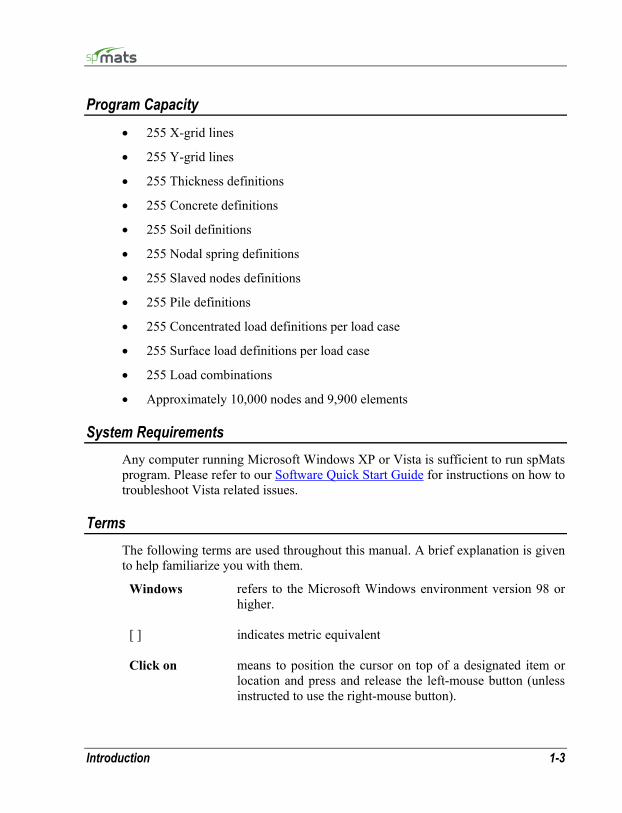
Program Capacity • 255 X-grid lines
• 255 Y-grid lines
• 255 Thickness definitions
• 255 Concrete definitions
• 255 Soil definitions
• 255 Nodal spring definitions
• 255 Slaved nodes definitions
• 255 Pile definitions
• 255 Concentrated load definitions per load case
• 255 Surface load definitions per load case
• 255 Load combinations
• Approximately 10,000 nodes and 9,900 elements
System Requirements Any computer running Microsoft Windows XP or Vista is sufficient to run spMats program. Please refer to our Software Quick Start Guide for instructions on how to troubleshoot Vista related issues.
Terms The following terms are used throughout this manual. A brief explanation is given to help familiarize you with them.
Windows refers to the Microsoft Windows environment version 98 or higher.
[ ] indicates metric equivalent
Click on means to position the cursor on top of a designated item or location and press and release the left-mouse button (unless instructed to use the right-mouse button).
1-4 Introduction
Double-click on means to position the cursor on top of a designated item or
location and press and release the left-mouse button twice in quick succession.
Marquee select means to depress the mouse button and continue to hold it down while moving the mouse. As you drag the mouse, a rectangle (known as a marquee) follows the cursor. Release the mouse button and the area inside the marquee is selected.
Conventions Various styles of text and layout have been used in this manual to help differentiate between different kinds of information. The styles and layout are explained below…
Italic indicates a glossary item, or emphasizes a given word or phrase.
Bold All bold typeface makes reference to either a menu or a menu item command such as File or Save, or a tab such as Description or Grid
Mono-space indicates something you should enter with the keyboard. For example type “c:\*.txt”.
KEY + KEY indicates a key combination. The plus sign indicates that you should press and hold the first key while pressing the second key, then release both keys. For example, “ALT + F” indicates that you should press the “ALT” key and hold it while you press the “F” key. then release both keys.
SMALL CAPS Indicates the name of an object such as a dialog box or a dialog box component. For example, the OPEN dialog box or the CANCEL or MODIFY buttons.
Installing, Purchasing and Licensing spMats For instructions on how to install, purchase and license StructurePoint software please refer to our Software Quick Start Guide.
Chapter 2 Method of Solution
spMats uses the Finite Element Method for the structural modeling and analysis of reinforced concrete slab systems or mat foundations subject to static loading conditions.
The slab is idealized as a mesh of rectangular elements interconnected at the corner nodes. The same mesh applies to the underlying soil with the soil stiffness concentrated at the nodes. Slabs of irregular geometry should be idealized to conform to geometry with rectangular boundaries. Even though slab and soil properties can vary from one element to another, they are assumed uniform within each element.
Three degrees of freedom are considered at each node, i.e. vertical translation and two rotations about the two orthogonal axes. An external load can exist in the direction of each of the above degrees of freedom, i.e., a vertical force and two moments about the Cartesian axes.
The Global Coordinate system The mid-surface of the slab lies in the XY plane of the right-handed XYZ orthogonal coordinate system shown in Figure 2-1. The slab thickness is measured in the direction of the Z-axis. Looking at the display monitor, the origin of the coordinate system is located in the bottom left corner of the screen. The positive X-axis points to the right, the positive Y-axis points upward towards the top of the monitor, and the positive Z-axis points out of the screen. Thus, the XY plane is defined as being the plane of the display monitor.
2-2 Method of Solution
YZ
Z
X X
YDisplayMonitor
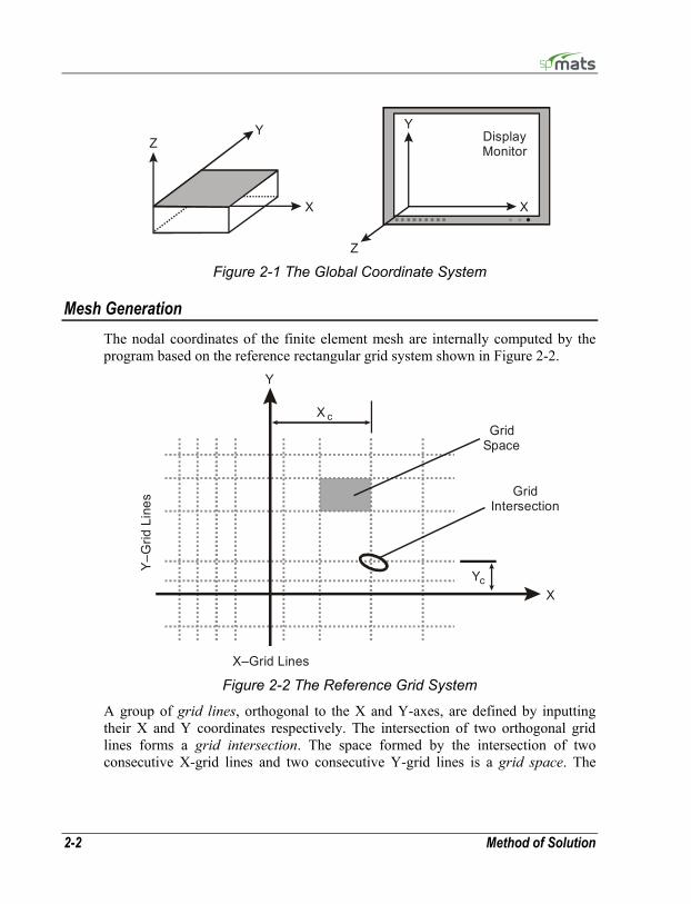
Figure 2-1 The Global Coordinate System
Mesh Generation The nodal coordinates of the finite element mesh are internally computed by the program based on the reference rectangular grid system shown in Figure 2-2.
Y
XY
X
c
cGrid
Space
GridIntersection
X–Grid Lines
Y–G
rid L
ines
Figure 2-2 The Reference Grid System
A group of grid lines, orthogonal to the X and Y-axes, are defined by inputting their X and Y coordinates respectively. The intersection of two orthogonal grid lines forms a grid intersection. The space formed by the intersection of two consecutive X-grid lines and two consecutive Y-grid lines is a grid space. The

Method of Solution 2-3
assignment of plate finite elements to the slab model is done by applying element thicknesses to the grid spaces.
Preparing the Input The first step in preparing the input is to draw a scaled plan view of the slab. The plan should include the boundaries slab, variations in the slab thickness and material properties, openings within the slab, and any variations in the soil sub-grade modulus. All superimposed loads applied on the slab should also be shown.
The next step is to superimpose a rectangular grid system over the plan of the slab. The following factors control the grid layout:
1. Grid lines must exist along slab boundaries and openings. Slab boundaries not parallel to the X- or Y-axis may be defined by steps that approximate the sloped boundary.
2. Grid lines must exist along the boundaries of slab thickness changes, slab material property changes, and soil property changes.
3. Grid lines must exist along boundaries of surface loads. 4. Grid lines must intersect at the locations of point loads and point supports. The above guidelines basically form the major grid lines, which produce the minimum number of finite elements for the particular mat geometry. The mesh can be refined by supplementing the model with minor grid lines between the major grid lines. Minor grid lines need to be added to achieve a uniform, well-graded mesh that produces results that will effectively capture the variations of the displacements and element forces. The location of the minor grid lines also depends on the level of accuracy that is desired from the analysis.
While the use of finer meshes will generally produce more accurate results, it will also require more solution time, computer memory, and disk space. Elements with with aspect ratios (length/width) near unity are generally expected to produce accurate results for regions having gradual changes of curvature. For slab regions where heavy concentrated forces are applied and where drastic changes in geometry exist, the use of finer element meshes may be required. Thus, in order to obtain a practical as well as accurate analytical solution, engineering judgment must be used.
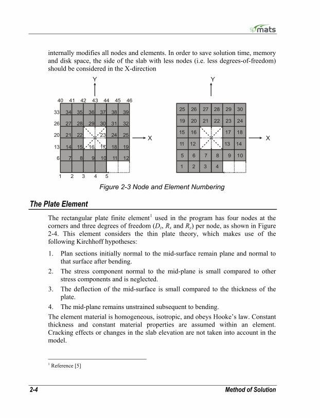
The member nodal incidences are internally computed by the program. All nodes and members are numbered from left to right (in the positive X-direction) and from bottom to top (in the positive Y-direction), as shown in Figure 2-3. When the reference grid system and/or assembling of elements is modified, the program
2-4 Method of Solution
internally modifies all nodes and elements. In order to save solution time, memory and disk space, the side of the slab with less nodes (i.e. less degrees-of-freedom) should be considered in the X-direction
Y Y
X X
1
6 7 8 9 10 11 12
11 12 13 14
15 16 17 18
65 7 8 9 10
2019 21 22 23 24
2625 27 28 29 30
13 14 15 16 17 18 19
20 21 22 23 24 25
26 27 28 29 30 31 32
33 34 35 36 37 38 39
40 41 42 43 44 45 46
2 3 4
1 2 3 4
5 Figure 2-3 Node and Element Numbering
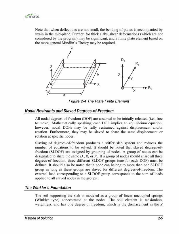
The Plate Element The rectangular plate finite element1 used in the program has four nodes at the corners and three degrees of freedom (Dz, Rx and Ry) per node, as shown in Figure 2-4. This element considers the thin plate theory, which makes use of the following Kirchhoff hypotheses:
1. Plan sections initially normal to the mid-surface remain plane and normal to that surface after bending.
2. The stress component normal to the mid-plane is small compared to other stress components and is neglected.
3. The deflection of the mid-surface is small compared to the thickness of the plate.
4. The mid-plane remains unstrained subsequent to bending. The element material is homogeneous, isotropic, and obeys Hooke’s law. Constant thickness and constant material properties are assumed within an element. Cracking effects or changes in the slab elevation are not taken into account in the model.
1 Reference [5]
Method of Solution 2-5
Note that when deflections are not small, the bending of plates is accompanied by strain in the mid-plane. Further, for thick slabs, shear deformations (which are not considered by the program) may be significant, and a finite plate element based on the more general Mindlin’s Theory may be required.
a
b
t
Z
Y
X
ZY
XR
RD
x
yz
Figure 2-4 The Plate Finite Element
Nodal Restraints and Slaved Degrees-of-Freedom All nodal degrees-of-freedom (DOF) are assumed to be initially released (i.e., free to move). Mathematically speaking, each DOF implies an equilibrium equation; however, nodal DOFs may be fully restrained against displacement and/or rotation. Furthermore, they may be slaved to share the same displacement or rotation at specific nodes.
Slaving of degrees-of-freedom produces a stiffer slab system and reduces the number of equations to be solved. It should be noted that slaved degrees-of-freedom (SLDOF) are assigned by grouping of nodes. A group of nodes can be designated to share the same Dz, Rx or Ry. If a group of nodes should share all three degrees-of-freedom, three different SLDOF groups (one for each DOF) must be defined. It should also be noted that a node can belong to more than one SLDOF group as long as these groups are slaved for different degrees-of-freedom. The external load corresponding to a SLDOF group corresponds to the sum of loads applied to all slaved nodes in the groups.
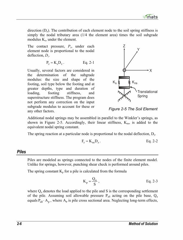
The Winkler’s Foundation The soil supporting the slab is modeled as a group of linear uncoupled springs (Winkler type) concentrated at the nodes. The soil element is tensionless, weightless, and has one degree of freedom, which is the displacement in the Z
2-6 Method of Solution
TranslationalSpring
ZY
X
KnsKs
Figure 2-5 The Soil Element
direction (Dz). The contribution of each element node to the soil spring stiffness is simply the nodal tributary area (1/4 the element area) times the soil subgrade modulus Ks, under the element.
The contact pressure, Pz, under each element node is proportional to the nodal deflection, Dz.
z s zP K D= . Eq. 2-1
Usually, several factors are considered in the determination of the subgrade modulus: the size and shape of the footing, soil type below the footing and at greater depths, type and duration of loading, footing stiffness, and superstructure stiffness. The program does not perform any correction on the input subgrade modulus to account for these or any other factors.
Additional nodal springs may be assembled in parallel to the Winkler’s springs, as shown in Figure 2-5. Accordingly, their linear stiffness, Kns, is added to the equivalent nodal spring constant.
The spring reaction at a particular node is proportional to the nodal deflection, Dz.
z ns zF K D= . Eq. 2-2
Piles Piles are modeled as springs connected to the nodes of the finite element model. Unlike for springs, however, punching shear check is performed around piles.
The spring constant Kp for a pile is calculated from the formula
up
QKS
= , Eq. 2-3
where Qu denotes the load applied to the pile and S is the corresponding settlement of the pile. Assuming soil allowable pressure Pall acting on the pile base, Qu equals all pP A⋅ , where Ap is pile cross sectional area. Neglecting long-term effects,
Method of Solution 2-7
the settlement of pile is estimated from the empirical formula for a single pile in cohesionless soil2:
u
p p
Q LDS100 A E
= + , Eq. 2-4
where D is pile diameter, L is pile length, and Ep is modulus of elasticity of pile material. The above formula is units independent as long as all its terms have consistent units. For noncircular piles an effective diameter is calculated from the formula
p4AD =
π. Eq. 2-5
The Nonlinear Solution The supporting soil is assumed to be tensionless. When tensile contact pressure (nodal uplift) occurs, an iterative procedure is used to eliminate the corresponding nodal spring stiffness contribution to the global stiffness of the entire slab/soil structural system and to re-solve the equilibrium equations.
A maximum number of iterations, as well as a maximum displacement limit, are the controlling parameters for the solution of the nonlinear problem. This iterative procedure is repeated for each load combination. When the limits are exceeded for a particular load combination, the program still attempts to solve for the remaining load combinations.
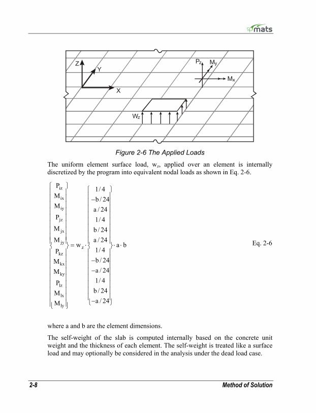
Types of Loads External loads are applied as concentrated nodal loads and/or element surface loads according to the sign convention shown in Figure 2-6.
A concentrated nodal load consists of a vertical load, Pz, and two concentrated moments about the X and Y axes, Mx and My. It should be noted that a positive vertical load is applied upward (in the positive Z-direction).
2 Reference [8]
2-8 Method of Solution
W
M
M
PZ
z
y
x
zY
X
Figure 2-6 The Applied Loads
The uniform element surface load, wz, applied over an element is internally discretized by the program into equivalent nodal loads as shown in Eq. 2-6.
Eq. 2-6
where a and b are the element dimensions.
The self-weight of the slab is computed internally based on the concrete unit weight and the thickness of each element. The self-weight is treated like a surface load and may optionally be considered in the analysis under the dead load case.
iz
ix
iy
jz
jx
jyz
kz
kx
ky
lz
lx
ly
P 1/ 4M b / 24M a / 24P 1/ 4
M b / 24M a / 24
w a b1/ 4Pb / 24Ma / 24M1/ 4Pb / 24Ma / 24M
⎧ ⎫ ⎧ ⎫⎪ ⎪ ⎪ ⎪⎪ ⎪ −⎪ ⎪⎪ ⎪ ⎪ ⎪⎪ ⎪ ⎪ ⎪⎪ ⎪ ⎪ ⎪⎪ ⎪ ⎪ ⎪⎪ ⎪ ⎪ ⎪⎪ ⎪⎪ ⎪ ⎪ ⎪= ⋅ ⋅ ⋅⎨ ⎬ ⎨ ⎬⎪ ⎪ ⎪ ⎪⎪ ⎪ ⎪ ⎪−⎪ ⎪ ⎪ ⎪
−⎪ ⎪ ⎪ ⎪⎪ ⎪ ⎪ ⎪⎪ ⎪ ⎪ ⎪⎪ ⎪ ⎪ ⎪⎪ ⎪ ⎪ ⎪−⎩ ⎭⎪ ⎪⎩ ⎭
Method of Solution 2-9
Load Cases and Combinations All applied loads are categorized into six load cases: A through F. Loads are applied to the slab under a load case. The slab is analyzed and designed under load combinations. A load combination is the algebraic sum of each of the load cases multiplied by a load factor.
Load combinations are categorized into Service level and Ultimate level. For each service level combination, the nodal deflections, element pressures, and nodal spring reactions are output. For an ultimate level combination, the element bending moments are output.
The Solution The solution process is summarized in the following steps:
1. Compute the plate element stiffness matrix 2. Compute the soil element stiffness matrix. 3. Assemble the global stiffness matrix. 4. Combine the applied loads based on the defined load combinations and form
the load vector. 5. Compute the displacement vector, U, by solving the equilibrium equation: K U F= , Eq. 2-7
where K is the structural stiffness matrix and F is the load vector.
6. If uplift is detected at any node (upward displacement), the soil contribution at that node is eliminated and the procedure (from step 2 above) is repeated. This is checked only if soil is present.
7. Compute the spring reactions and soil pressures (service combinations only). 8. Compute the moments at the element nodes (ultimate combinations only). 9. Repeat steps 4 through 8 for each combination. 10. For all service level combinations, envelopes are computed for displacements,
pressures, and spring reactions. 11. For all ultimate level combinations, the element bending moment envelopes
are computed along with the corresponding required area of reinforcing steel.
2-10 Method of Solution
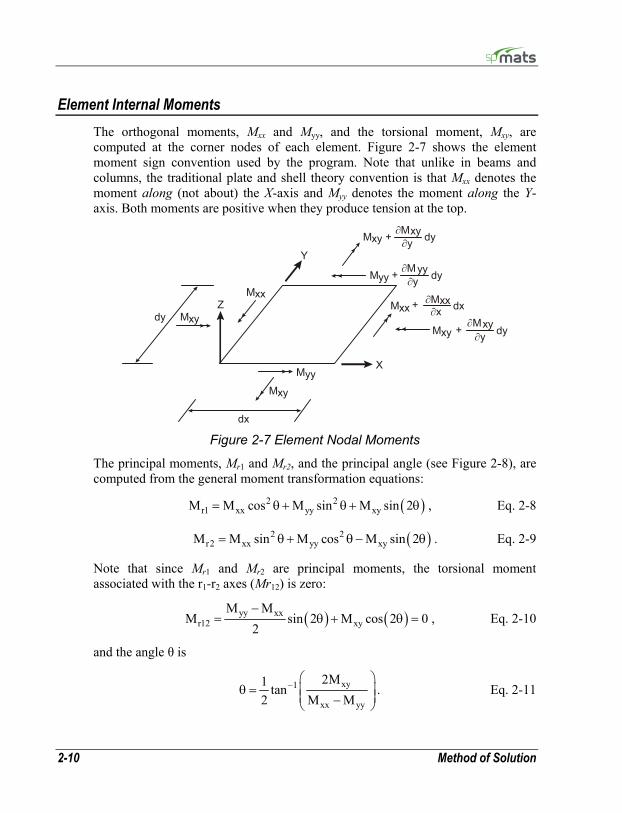
Element Internal Moments The orthogonal moments, Mxx and Myy, and the torsional moment, Mxy, are computed at the corner nodes of each element. Figure 2-7 shows the element moment sign convention used by the program. Note that unlike in beams and columns, the traditional plate and shell theory convention is that Mxx denotes the moment along (not about) the X-axis and Myy denotes the moment along the Y-axis. Both moments are positive when they produce tension at the top.
Mxx
MyyMxy
Mxy
Y
dy
X
dx
Z
Mxy dy ∂y∂Mxy +
∂MxxMxx dx∂x+
∂MxyMxy dy∂y+
∂MyyMyy dy∂y+
Figure 2-7 Element Nodal Moments
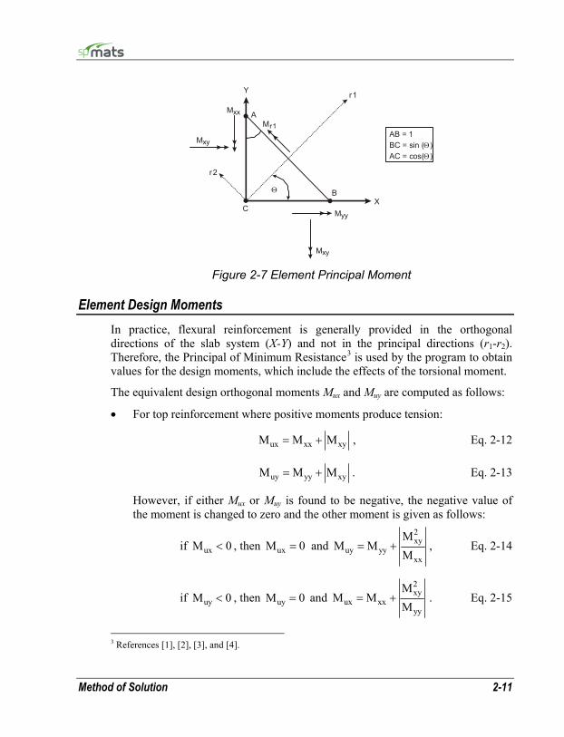
The principal moments, Mr1 and Mr2, and the principal angle (see Figure 2-8), are computed from the general moment transformation equations:
( )2 2r1 xx yy xyM M cos M sin M sin 2= θ + θ + θ , Eq. 2-8
( )2 2r2 xx yy xyM M sin M cos M sin 2= θ + θ − θ . Eq. 2-9
Note that since Mr1 and Mr2 are principal moments, the torsional moment associated with the r1-r2 axes (Mr12) is zero:
( ) ( )yy xxr12 xy
M MM sin 2 M cos 2 0
2−
= θ + θ = , Eq. 2-10
and the angle θ is
xy1
xx yy
2M1 tan2 M M
− ⎛ ⎞θ = ⎜ ⎟⎜ ⎟−⎝ ⎠
. Eq. 2-11
Method of Solution 2-11
Mxy
Mxy
Mxx
Myy
X
r2
Mr1
r1
C
B
Y
A
AB = 1BC = sin ( )ΘAC = cos( )Θ
Θ
Figure 2-7 Element Principal Moment
Element Design Moments In practice, flexural reinforcement is generally provided in the orthogonal directions of the slab system (X-Y) and not in the principal directions (r1-r2). Therefore, the Principal of Minimum Resistance3 is used by the program to obtain values for the design moments, which include the effects of the torsional moment.
The equivalent design orthogonal moments Mux and Muy are computed as follows:
• For top reinforcement where positive moments produce tension:
ux xx xyM M M= + , Eq. 2-12
uy yy xyM M M= + . Eq. 2-13
However, if either Mux or Muy is found to be negative, the negative value of the moment is changed to zero and the other moment is given as follows:
if uxM 0< , then uxM 0= and 2xy
uy yyxx
MM M
M= + , Eq. 2-14
if uyM 0< , then uyM 0= and 2xy
ux xxyy
MM M
M= + . Eq. 2-15
3 References [1], [2], [3], and [4].
2-12 Method of Solution
• For bottom reinforcement where negative moments produce tension:
ux xx xyM M M= − , Eq. 2-16
uy yy xyM M M= − . Eq. 2-17
However, if either Mux or Muy is found to be positive, the positive value of the moment is changed to zero and the other moment is given as follows:
if uxM 0> , then uxM 0= and 2xy
uy yyxx
MM M
M= − , Eq. 2-18
if uyM 0> , then uyM 0= and 2xy
ux xxyy
MM M
M= − . Eq. 2-19
In the above equations, Mxx, Myy and Mxy correspond to the maximum principal moment obtained from all nodes and all ultimate load combinations.
Required Reinforcement The required area of reinforcing steel is computed based on a rectangular section with no compression reinforcement and one layer of tension reinforcement. The assumptions and limits used conform to the design specifications based on the accepted Strength Design Method and Unified Design Provisions.
The maximum usable strain at the extreme concrete compression fiber is 0.003 for ACI standards and 0.0035 for CSA standards. The rectangular concrete stress block is assumed with the block depth equal to:
1a c= β , Eq. 2-20
where c is the distance from the extreme compression fiber to the neutral axis and factor 1β equals
'1 c0.65 1.05 0.05f 0.85≤ β = − ≤ Eq. 2-21
for ACI standards and
'1 c0.67 1.05 0.025f≤ β = − Eq. 2-22
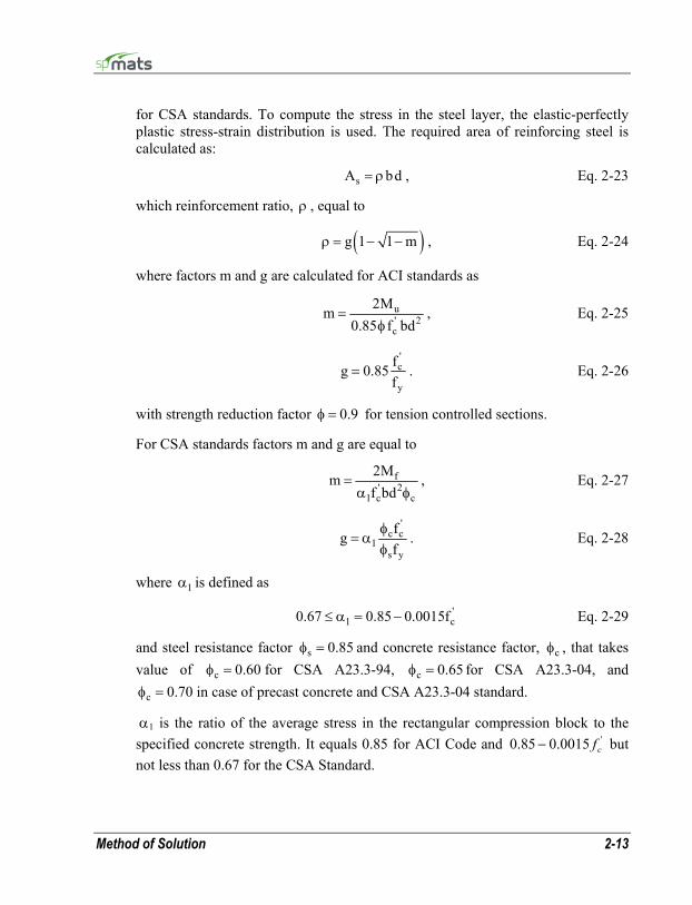
Method of Solution 2-13
for CSA standards. To compute the stress in the steel layer, the elastic-perfectly plastic stress-strain distribution is used. The required area of reinforcing steel is calculated as:
sA bd= ρ , Eq. 2-23
which reinforcement ratio, ρ , equal to
( )g 1 1 mρ = − − , Eq. 2-24
where factors m and g are calculated for ACI standards as
u' 2c
2Mm0.85 f bd
=φ
, Eq. 2-25
'c
y
fg 0.85f
= . Eq. 2-26
with strength reduction factor 0.9φ = for tension controlled sections.
For CSA standards factors m and g are equal to
f' 2
1 c c
2Mmf bd
=α φ
, Eq. 2-27
'
c c1
s y
fgf
φ= α
φ. Eq. 2-28
where 1α is defined as
'1 c0.67 0.85 0.0015f≤ α = − Eq. 2-29
and steel resistance factor s 0.85φ = and concrete resistance factor, cφ , that takes value of c 0.60φ = for CSA A23.3-94, c 0.65φ = for CSA A23.3-04, and
c 0.70φ = in case of precast concrete and CSA A23.3-04 standard.
α1 is the ratio of the average stress in the rectangular compression block to the specified concrete strength. It equals 0.85 for ACI Code and '0015.085.0 cf− but not less than 0.67 for the CSA Standard.
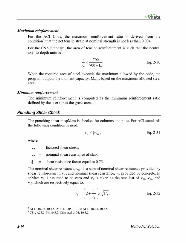
2-14 Method of Solution
Maximum reinforcement For the ACI Code, the maximum reinforcement ratio is derived from the condition4 that the net tensile strain at nominal strength is not less than 0.004.
For the CSA Standard, the area of tension reinforcement is such that the neutral axis-to-depth ratio is5:
y
c 700d 700 f
<+
Eq. 2-30
When the required area of steel exceeds the maximum allowed by the code, the program outputs the moment capacity, Mmax, based on the maximum allowed steel area.
Minimum reinforcement The minimum reinforcement is computed as the minimum reinforcement ratio defined by the user times the gross area.
Punching Shear Check The punching shear in spMats is checked for columns and piles. For ACI standards the following condition is used:
u nv v≤ φ , Eq. 2-31
where
vu = factored shear stress,
vn = nominal shear resistance of slab,
φ = shear resistance factor equal to 0.75. The nominal shear resistance, vn , is a sum of nominal shear resistance provided by shear reinforcement, vs , and nominal shear resistance, vc, provided by concrete. In spMats vs is assumed to be zero and vc is taken as the smallest of vc1, vc2, and vc3.which are respectively equal to:
c1 cc
4v 2 f '⎛ ⎞
= + λ⎜ ⎟β⎝ ⎠, Eq. 2-32
4 ACI 318-02, 10.3.5; ACI 318-05, 10.3.5; ACI 318-08, 10.3.5 5 CSA A23.3-94, 10.5.2, CSA A23.3-04, 10.5.2
Method of Solution 2-15
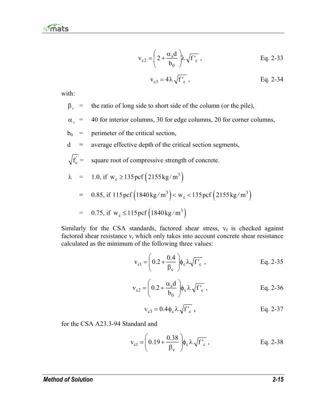
sc2 c
0
dv 2 f 'b
⎛ ⎞α= + λ⎜ ⎟
⎝ ⎠, Eq. 2-33
c3 cv 4 f '= λ , Eq. 2-34
with:
cβ = the ratio of long side to short side of the column (or the pile),
sα = 40 for interior columns, 30 for edge columns, 20 for corner columns,
b0 = perimeter of the critical section,
d = average effective depth of the critical section segments,
'cf = square root of compressive strength of concrete.
λ = 1.0, if ( )3cw 135pcf 2155kg / m≥
= 0.85, if ( ) ( )3 3c115pcf 1840kg / m w 135pcf 2155kg / m< <
= 0.75, if ( )3cw 115pcf 1840kg / m≤
Similarly for the CSA standards, factored shear stress, vf is checked against factored shear resistance vr which only takes into account concrete shear resistance calculated as the minimum of the following three values:
c1 c cc
0.4v 0.2 f '⎛ ⎞
= + φ λ⎜ ⎟β⎝ ⎠, Eq. 2-35
sc2 c c
0
dv 0.2 f 'b
⎛ ⎞α= + φ λ⎜ ⎟
⎝ ⎠, Eq. 2-36
c3 c cv 0.4 f '= φ λ , Eq. 2-37
for the CSA A23.3-94 Standard and
c1 c cc
0.38v 0.19 f '⎛ ⎞
= + φ λ⎜ ⎟β⎝ ⎠, Eq. 2-38

2-16 Method of Solution
sc2 c c
0
dv 0.19 f 'b
⎛ ⎞α= + φ λ⎜ ⎟
⎝ ⎠, Eq. 2-39
c3 c cv 0.38 f '= φ λ , Eq. 2-40
for the CSA A23.3-04 Standard. Factor sα equals 4 for interior columns, 3 for edge columns, and 2 for corner columns for both CSA standards. Factor λ accounts for low density concrete and is equal to
λ = 1.0, if ( )3cw 2150kg / m 134.2pcf≥
= 0.85, if ( ) ( )3 3c1850kg / m 115.5pcf w 2150kg / m 134.2pcf< <
= 0.75, if ( )3cw 1850kg / m 115.5pcf≤
Also, for interior column and piles, the value of effective depth, d, in Eq. 2-38 through 2-40 will be multiplied by factor1300 /(1000 d)+ .
The projection of the critical section to the middle surface of the slab is a polygon located so its perimeter b0 is a minimum and the distance between its segments and the column is not less than a half of slab effective depth. For circular column and piles, the critical section is approximated by a polygon with ten segments per quarter. The depth of each segment can be different depending on the depth of the slab at the location of the segment. In the case of edge or corner columns and piles, segments of the critical section that lie outside of the slab are disregarded.
For such defined section the area Ac, the coordinates { }c cx , y of the centroid, and Jxx, Jyy, Jxy properties are calculated. Force (Puz) and moments (Mux and Muy) applied at the center of the column (pile) are transformed to the centroid of the critical section. The unbalanced moments to be transferred by eccentricity of shear are:
vx vx ux uz f cM (M P (y y ))= γ + − , Eq. 2-41
vy vy uy uz f cM (M P (x x ))= γ − − , Eq. 2-42
where xf, yf are the coordinates of the column (pile) center. If Bx and By denote the dimensions of the critical section then the fractions of the unbalanced moments transferred by eccentricity of shear can be calculated as
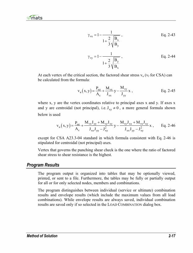
Method of Solution 2-17
vxx
y
11B21
3 B
γ = −+
, Eq. 2-43
vyy
x
11B21
3 B
γ = −
+
, Eq. 2-44
At each vertex of the critical section, the factored shear stress vu (vf for CSA) can be calculated from the formula:
( ) vyuz vxu
c xx yy
MP Mv x, y y xA J J
= + − , Eq. 2-45
where x, y are the vertex coordinates relative to principal axes x and y. If axes x and y are centroidal (not principal), i.e. xyJ 0≠ , a more general formula shown below is used
( ) vx yy vy xy vy xx vx xyuzu 2 2
c xx yy xy xx yy xy
M J M J M J M JPv x, y y xA J J J J J J
+ += + −
− −, Eq. 2-46
except for CSA A23.3-04 standard in which formula consistent with Eq. 2-46 is stipulated for centroidal (not principal) axes.
Vertex that governs the punching shear check is the one where the ratio of factored shear stress to shear resistance is the highest.
Program Results The program output is organized into tables that may be optionally viewed, printed, or sent to a file. Furthermore, the tables may be fully or partially output for all or for only selected nodes, members and combinations.
The program distinguishes between individual (service or ultimate) combination results and envelope results (which include the maximum values from all load combinations). While envelope results are always saved, individual combination results are saved only if so selected in the LOAD COMBINATION dialog box.
2-18 Method of Solution
Load Vector: This table is output for individual ultimate load combinations. It lists the nodal load vector that is actually used by the program for each load combination. The axial force, Fz, moment about X, Mx, and moment about Y, My, at each node includes the factored dead, live and lateral forces at the node, including the discretized effects of uniform surface loads. Positive forces are applied in the direction of the positive Z-axis (upward) and positive moments are determined using the right-hand rule.
Nodal Displacements and Rotations: This table is output for individual service and individual ultimate load combinations. It lists the displacement vector for each load combination. The table lists the displacement, Dz, and the two rotations about the X and Y-axis, Rx and Ry, respectively. Positive displacement is in the positive Z-direction, and the right-hand rule is used to determine the direction of the rotations.
Nodal Spring Displacements and Reactions: This table is output for individual service load combinations. For the nodes with specified nodal springs, the displacement and reaction are listed. Since the soil is assumed tensionless, the pressure is set to zero for positive (upward) displacements.
Element Soil Displacements and Pressures: This table is output for individual service load combinations. For the elements with specified soil, the displacement and pressure at all four nodes are listed. Since the soil is assumed tensionless, the pressure is set to zero for positive (upward) displacements.
Element Nodal Moments: This table is output for individual ultimate load combinations. It lists, at each of the element four nodes (i, j, k and l), the orthogonal moments (Mxx and Myy), the torsional moment (Mxy) and the equivalent principal moments (Mr1 and Mr2), along with the principal angle. Note that Mxx and Myy are positive when they produce tension at the top and are referred to as moments along the X and Y-axes, respectively. For more information about these moments and the sign convention, see “Element Nodal Moments” earlier in this chapter.

Method of Solution 2-19
Nodal Displacement Envelopes: This table lists the maximum vertical displacement, Dz, from all service load combinations, along with the governing combination. Again, positive displacements are upward in the positive Z-direction.
Nodal Spring Displacement and Reaction Envelopes: For the nodes with specified nodal springs, this table lists the maximum displacements and reactions resulting from all service load combinations. The governing load combination is listed.
Element Soil Displacement and Pressure Envelopes: For the elements with specified soil, this table lists the maximum displacements and pressures resulting from all service load combinations and all four element nodes. The governing load combination and the governing element node are also listed.
Element Top Moment Envelopes: For each element, the maximum nodal principal moment (Mr1) producing tension at the top resulting from all ultimate load combinations and all for element nodes is listed. The governing load combination and the governing element node are also listed, along with the corresponding nodal moments (Mxx, Myy and Mxy) and the directional angle.
Element Bottom Design Moment and Reinforcement: For each element, the maximum nodal principal moment (Mr1) producing tension at the bottom resulting from all ultimate load combinations and all four element nodes is listed. The governing load combination and the governing element node are also listed along with the corresponding nodal moments (Mxx, Myy and Mxy) and the directional angle.
Element Top Design Moment and Reinforcement: For each element, the maximum nodal principal moment (Mr1) producing tension at the top resulting from all ultimate load combinations and all four element nodes is listed. The governing load combination and the governing element node are also listed along with the corresponding directional angle and the required area of skewed reinforcement. The equivalent design orthogonal moment (Mux and Muy) with the required area of reinforcing steel is also listed (see “Element Design Moments” earlier in this chapter). If the required area of reinforcing steel exceeds
2-20 Method of Solution
the maximum allowed by the code, the ratio of the ultimate moment to the maximum moment capacity, (in percent), is reported instead.
Punching Shear : For each column and pile, punching shear stresses resulting from ultimate load combinations are listed. For each ultimate load combination, the report includes geometrical properties of critical sections and shear stresses at critical points, i.e. vertexes at which the ratios of factored shear stress to shear resistance are the highest.
References [1] Wood, R.H., “The Reinforcement of Slabs in Accordance with a
Predetermined Field of Moments,” Concrete, February 1968. [2] Mills, H.B., Armer, G.S.T. and Wood, R.H., Correspondence regarding
Article “The Reinforcement of Slabs in Accordance with Predetermined Field Moment,” Concrete, August 1968.
[3] Gupta, A.K., and Sen Siddhartha, “Design of Flexural Reinforcement in Concrete Slabs,” Journal of the Structural Division, ASCE, Vol. 103, No. St4, April 1972.
[4] Park, R. and Gamble, W.L., Reinforced Concrete Slabs, John Wiley & Sons, 2000. (Chapter 5, Section 5-4) pp. 207-231.
[5] Zienkiewicz, O.C. and Taylor, R.L., The Finite Element Method, McGraw-Hill Book Company, Fourth Edition, 1988.
[6] Bowles, Joseph F., Foundation Analysis and Design, McGraw-Hill Book Company, Fifth Edition, 1996
[7] ACI 336.2R-88, “Suggested Analysis and Design Procedures for Combined Footings and Mats.”
[8] Prakash, S., and Sharma, H.D., Pile Foundations in Engineering Practice, John Wiley & Sons, 1990, pp. 251.
[9] Building Code Requirements for Structural Concrete (ACI 318-08) and Commentary (ACI 318R-08), American Concrete Institute, 2008
[10] Building Code Requirements for Structural Concrete (ACI 318-05) and Commentary (ACI 318R-05), American Concrete Institute, 2005
[11] Building Code Requirements for Structural Concrete (ACI 318-02) and Commentary (ACI 318R-02), American Concrete Institute, 2002
[12] A23.3-04, Design of Concrete Structures, Canadian Standards Association, 2004
[13] A23.3-94, Design of Concrete Structures, Canadian Standards Association, 1994 (Reaffirmed 2000)
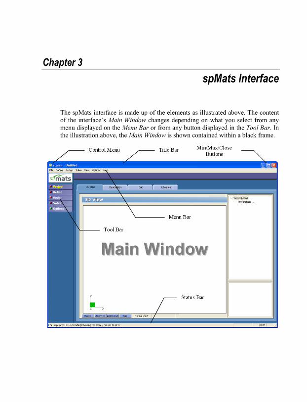
Chapter 3 spMats Interface
The spMats interface is made up of the elements as illustrated above. The content of the interface’s Main Window changes depending on what you select from any menu displayed on the Menu Bar or from any button displayed in the Tool Bar. In the illustration above, the Main Window is shown contained within a black frame.
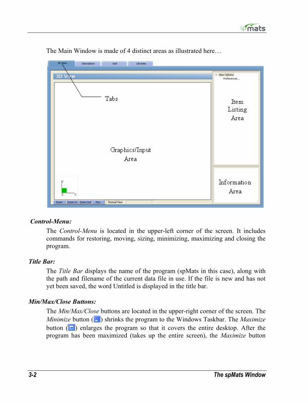
3-2 The spMats Window
The Main Window is made of 4 distinct areas as illustrated here…
Control-Menu: The Control-Menu is located in the upper-left corner of the screen. It includes commands for restoring, moving, sizing, minimizing, maximizing and closing the program.
Title Bar: The Title Bar displays the name of the program (spMats in this case), along with the path and filename of the current data file in use. If the file is new and has not yet been saved, the word Untitled is displayed in the title bar.
Min/Max/Close Buttons: The Min/Max/Close buttons are located in the upper-right corner of the screen. The Minimize button ( ) shrinks the program to the Windows Taskbar. The Maximize button ( ) enlarges the program so that it covers the entire desktop. After the program has been maximized (takes up the entire screen), the Maximize button
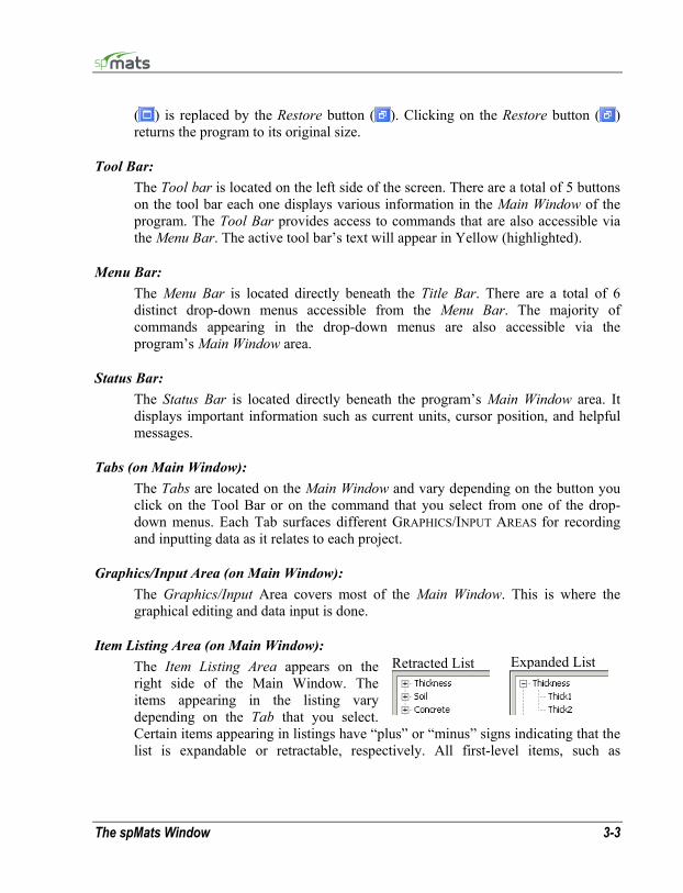
The spMats Window 3-3
( ) is replaced by the Restore button ( ). Clicking on the Restore button ( ) returns the program to its original size.
Tool Bar: The Tool bar is located on the left side of the screen. There are a total of 5 buttons on the tool bar each one displays various information in the Main Window of the program. The Tool Bar provides access to commands that are also accessible via the Menu Bar. The active tool bar’s text will appear in Yellow (highlighted).
Menu Bar: The Menu Bar is located directly beneath the Title Bar. There are a total of 6 distinct drop-down menus accessible from the Menu Bar. The majority of commands appearing in the drop-down menus are also accessible via the program’s Main Window area.
Status Bar: The Status Bar is located directly beneath the program’s Main Window area. It displays important information such as current units, cursor position, and helpful messages.
Tabs (on Main Window): The Tabs are located on the Main Window and vary depending on the button you click on the Tool Bar or on the command that you select from one of the drop-down menus. Each Tab surfaces different GRAPHICS/INPUT AREAS for recording and inputting data as it relates to each project.
Graphics/Input Area (on Main Window): The Graphics/Input Area covers most of the Main Window. This is where the graphical editing and data input is done.
Item Listing Area (on Main Window): The Item Listing Area appears on the right side of the Main Window. The items appearing in the listing vary depending on the Tab that you select. Certain items appearing in listings have “plus” or “minus” signs indicating that the list is expandable or retractable, respectively. All first-level items, such as
Retracted List Expanded List
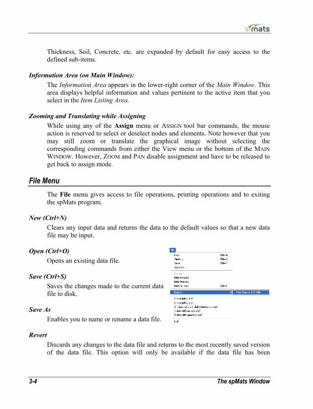
3-4 The spMats Window
Thickness, Soil, Concrete, etc. are expanded by default for easy access to the defined sub-items.
Information Area (on Main Window): The Information Area appears in the lower-right corner of the Main Window. This area displays helpful information and values pertinent to the active item that you select in the Item Listing Area.
Zooming and Translating while Assigning While using any of the Assign menu or ASSIGN tool bar commands, the mouse action is reserved to select or deselect nodes and elements. Note however that you may still zoom or translate the graphical image without selecting the corresponding commands from either the View menu or the bottom of the MAIN WINDOW. However, ZOOM and PAN disable assignment and have to be released to get back to assign mode.
File Menu The File menu gives access to file operations, printing operations and to exiting the spMats program.
New (Ctrl+N) Clears any input data and returns the data to the default values so that a new data file may be input.
Open (Ctrl+O) Opens an existing data file.
Save (Ctrl+S) Saves the changes made to the current data file to disk.
Save As Enables you to name or rename a data file.
Revert Discards any changes to the data file and returns to the most recently saved version of the data file. This option will only be available if the data file has been

The spMats Window 3-5
previously saved and there have been modifications done on the data file since. Do not save the data file immediately prior to reverting otherwise you will revert to nothing.
Print Results Provides a printout of the input and output data.
Print Screen (Ctrl+P) Prints the graphical image displayed in the GRAPHICS/INPUT AREA of the MAIN WINDOW.
Export | Mat Plan to DXF File… Exports mat plan view to a DXF file for easier integration with drafting and modeling software.
Exit Ends the spMats program.
Define Menu The Define menu provides access to commands used to define all of the input data. The information you input via the commands found under the Define menu will be used when assigning, and for calculating and designing the slab.
General Info Defines and records the particulars on the project including project name and description, project date and time, and engineering parameters including units of measure and design code.
Grid Defines the grid lines that make up the rectangular grid system. The slab model is defined based on the grid system specified here. This command also gives access to the grid preferences where you are able to show/hide node and element numbers, select between dotted or solid grid lines, and specify the coordinate precision.

3-6 The spMats Window
Library Provides access to libraries from which data items can be imported to the current project or where data items can be recorded so they can be used in other projects.
Thickness Defines the plate element thickness entries.
Concrete Defines the concrete material properties including compressive strength, unit weight, Young’s modulus and Poisson’s ratio.
Soil Defines soil properties including subgrade modulus and allowable pressure.
Reinforcing Steel Defines reinforcing steel material properties including yield strength and Young’s modulus.
Design Parameters Defines the parameters that set the criteria for designing the slab. These parameters include minimum reinforcement ratio and distance of reinforcement from top and from bottom in both directions.
Columns Defines column properties including type and cross section dimensions.
Nodal Springs Defines nodal spring entries including the spring constant (K).
Slaved Nodes Defines slaved nodes and their respective degrees of freedom (Dz, Rx, Ry).
Piles Defines pile properties including pile type, cross section dimensions, pile length, material properties, and soil. These properties are used to calculate the equivalent spring constant for a pile.
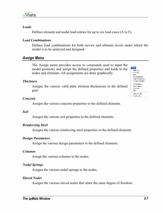
The spMats Window 3-7
Loads Defines element and nodal load entries for up to six load cases (A to F).
Load Combinations Defines load combinations for both service and ultimate levels under which the model is to be analyzed and designed.
Assign Menu The Assign menu provides access to commands used to input the model geometry and assign the defined properties and loads to the nodes and elements. All assignments are done graphically.
Thickness Assigns the various valid plate element thicknesses to the defined grid.
Concrete Assigns the various concrete properties to the defined elements.
Soil Assigns the various soil properties to the defined elements.
Reinforcing Steel Assigns the various reinforcing steel properties to the defined elements.
Design Parameters Assign the various design parameters to the defined elements.
Columns Assign the various columns to the nodes.
Nodal Springs Assigns the various nodal springs to the nodes.
Slaved Nodes Assigns the various slaved nodes that share the same degree of freedom.
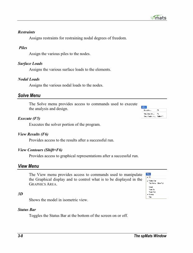
3-8 The spMats Window
Restraints Assigns restraints for restraining nodal degrees of freedom.
Piles Assign the various piles to the nodes.
Surface Loads Assigns the various surface loads to the elements.
Nodal Loads Assigns the various nodal loads to the nodes.
Solve Menu The Solve menu provides access to commands used to execute the analysis and design.
Execute (F5) Executes the solver portion of the program.
View Results (F6) Provides access to the results after a successful run.
View Contours (Shift+F6) Provides access to graphical representations after a successful run.
View Menu The View menu provides access to commands used to manipulate the Graphical display and to control what is to be displayed in the GRAPHICS AREA.
3D Shows the model in isometric view.
Status Bar Toggles the Status Bar at the bottom of the screen on or off.
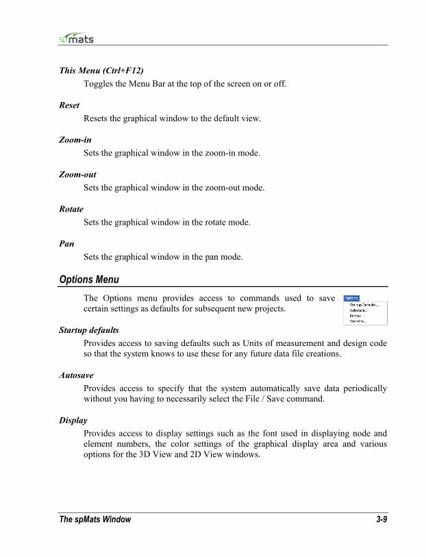
The spMats Window 3-9
This Menu (Ctrl+F12) Toggles the Menu Bar at the top of the screen on or off.
Reset Resets the graphical window to the default view.
Zoom-in Sets the graphical window in the zoom-in mode.
Zoom-out Sets the graphical window in the zoom-out mode.
Rotate Sets the graphical window in the rotate mode.
Pan Sets the graphical window in the pan mode.
Options Menu The Options menu provides access to commands used to save certain settings as defaults for subsequent new projects.
Startup defaults Provides access to saving defaults such as Units of measurement and design code so that the system knows to use these for any future data file creations.
Autosave Provides access to specify that the system automatically save data periodically without you having to necessarily select the File / Save command.
Display Provides access to display settings such as the font used in displaying node and element numbers, the color settings of the graphical display area and various options for the 3D View and 2D View windows.

3-10 The spMats Window
Statistics Provides access to information such as total number of nodes, elements, and definitions.
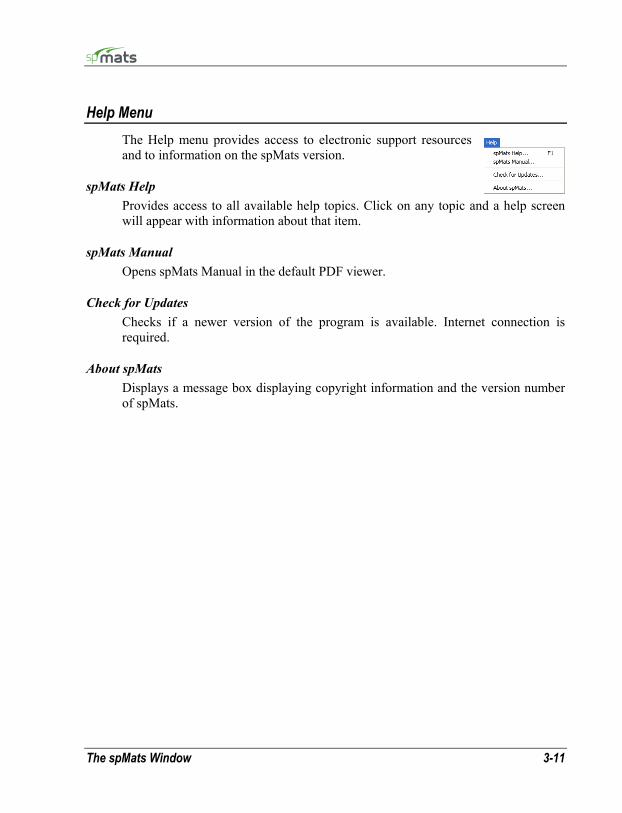
The spMats Window 3-11
Help Menu The Help menu provides access to electronic support resources and to information on the spMats version.
spMats Help Provides access to all available help topics. Click on any topic and a help screen will appear with information about that item.
spMats Manual Opens spMats Manual in the default PDF viewer.
Check for Updates Checks if a newer version of the program is available. Internet connection is required.
About spMats Displays a message box displaying copyright information and the version number of spMats.


Chapter 4 Operating spMats
In this chapter, the sections follow the order in which commands and options appear under the subsequent menu items.
We begin with those found under the File menu and end with those under the Help menu.
Many of the commands and options that appear under these menus are also accessible by other methods. Consequently, these other methods are also explained.
Creating a New Data File When spMats is first loaded, the program is ready to begin receiving input for a new project. Unless you save the file, the data will not have a filename associated with it, and the title bar will display the word Untitled as illustrated here…
• From the File menu, choose New. This clears the screen in preparation for a
new project or data entry file and returns the program to its default settings.
• If existing data on an open project has been changed prior to executing the New command, the program will display the following message box inquiring whether you wish to save the data on the open project or data file before creating a new file…
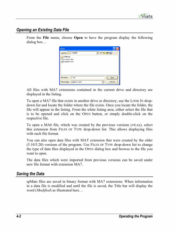
4-2 Operating the Program
Opening an Existing Data File From the File menu, choose Open to have the program display the following dialog box…
All files with MA7 extensions contained in the current drive and directory are displayed in the listing.
To open a MA7 file that exists in another drive or directory, use the LOOK IN drop-down list and locate the folder where the file exists. Once you locate the folder, the file will appear in the listing. From the white listing area, either select the file that is to be opened and click on the OPEN button, or simply double-click on the respective file.
To open a MA6 file, which was created by the previous versions (v6.xx), select this extension from FILES OF TYPE drop-down list. This allows displaying files with such file format.
You can also open data files with MAT extension that were created by the older (5.10/5.20) versions of the program. Use FILES OF TYPE drop-down list to change the type of data files displayed in the OPEN dialog box and browse to the file you want to open.
The data files which were imported from previous versions can be saved under new file format with extension MA7.
Saving the Data spMats files are saved in binary format with MA7 extensions. When information in a data file is modified and until the file is saved, the Title bar will display the word (Modified) as illustrated here…
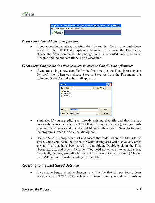
Operating the Program 4-3
To save your data with the same filename: • If you are editing an already existing data file and that file has previously been
saved (i.e. the TITLE BAR displays a filename), then from the File menu, choose the Save command. The changes will be recorded under the same filename and the old data file will be overwritten.
To save your data for the first time or to give an existing data file a new filename: • If you are saving a new data file for the first time (i.e. the TITLE BAR displays
Untitled), then when you choose Save or Save As from the File menu, the following SAVE AS dialog box will appear…
• Similarly, If you are editing an already existing data file and that file has
previously been saved (i.e. the TITLE BAR displays a filename), and you wish to record the changes under a different filename, then choose Save As to have the program surface the SAVE AS dialog box.
• Use the SAVE IN drop-down list and locate the folder where the file is to be saved. Once you locate the folder, the white listing area will display any other spMats files that have been saved in that folder. Double-click in the FILE NAME text box and type a filename. (You need not enter an extension since, by default, the program will affix the MA7 extension to the filename.) Choose the SAVE button to finish recording the data file.
Reverting to the Last Saved Data File • If you have begun to make changes to a data file that has previously been
saved, (i.e. the TITLE BAR displays a filename), and you suddenly wish to
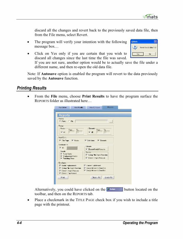
4-4 Operating the Program
discard all the changes and revert back to the previously saved data file, then from the File menu, select Revert.
• The program will verify your intention with the following message box…
• Click on Yes only if you are certain that you wish to discard all changes since the last time the file was saved. If you are not sure, another option would be to actually save the file under a different name, and then re-open the old data file.
Note: If Autosave option is enabled the program will revert to the data previously saved by the Autosave function.
Printing Results • From the File menu, choose Print Results to have the program surface the
REPORTS folder as illustrated here…
Alternatively, you could have clicked on the button located on the toolbar, and then on the REPORTS tab.
• Place a checkmark in the TITLE PAGE check box if you wish to include a title page with the printout.

Operating the Program 4-5
From the RANGE group, you may select the range of nodes and elements to be printed for each of the tabular output blocks. NODES: Will print all or selected nodal data including coordinates, assignments and loads. ELEMENTS: Will print all or selected element indexes, assignments and loads.
• From the INPUT ECHO group, you may select the tables to be printed…
DEFINITIONS: Will print all the input data entered using the Define menu commands.
• Select the RESULTS to be printed. (Force Vector and/or displacement Vector) For more information about the output tables, see Program Results in Chapter 2.
• In the SERVICE group, select whether to display SPRING DISPLACEMENT & REACTIONS and/or ELEMENT DISPLACEMENT & PRESSURE. If check marked, the program will display the respective results under the service load calculations.
• In the ULTIMATE group, select whether to display ELEMENT NODAL MOMENTS. If check marked, the program will display the respective results under the ultimate load calculations.
• Place a check mark in PUNCHING SHEAR if you wish the output to include the respective results of the Punching Shear computations.
• In the NODES and ELEMENTS groups, select the ALL check box for a comprehensive output. For selective printing, specify the range of nodes and/or elements to print for.
• In the COMBINATIONS group, select ALL to print for all service and ultimate load combinations. To print for specific combinations, choose the SELECT button to have the program surface the following dialog box…
• Highlight the combinations from the DEFINED COMBINATIONS list, and click on the button to move them to the SELECTED COMBINATIONS list. Repeat
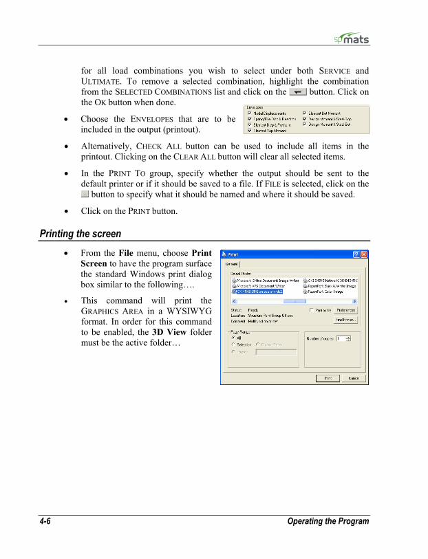
4-6 Operating the Program
for all load combinations you wish to select under both SERVICE and ULTIMATE. To remove a selected combination, highlight the combination from the SELECTED COMBINATIONS list and click on the button. Click on the OK button when done.
• Choose the ENVELOPES that are to be included in the output (printout).
• Alternatively, CHECK ALL button can be used to include all items in the printout. Clicking on the CLEAR ALL button will clear all selected items.
• In the PRINT TO group, specify whether the output should be sent to the default printer or if it should be saved to a file. If FILE is selected, click on the
button to specify what it should be named and where it should be saved.
• Click on the PRINT button.
Printing the screen • From the File menu, choose Print
Screen to have the program surface the standard Windows print dialog box similar to the following….
• This command will print the GRAPHICS AREA in a WYSIWYG format. In order for this command to be enabled, the 3D View folder must be the active folder…
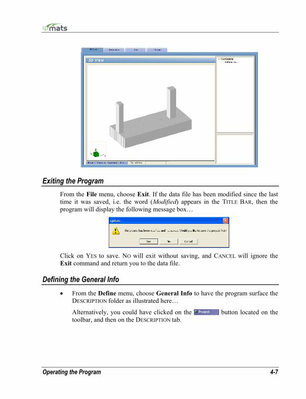
Operating the Program 4-7
Exiting the Program From the File menu, choose Exit. If the data file has been modified since the last time it was saved, i.e. the word (Modified) appears in the TITLE BAR, then the program will display the following message box…
Click on YES to save. NO will exit without saving, and CANCEL will ignore the Exit command and return you to the data file.
Defining the General Info • From the Define menu, choose General Info to have the program surface the
DESCRIPTION folder as illustrated here…
Alternatively, you could have clicked on the button located on the toolbar, and then on the DESCRIPTION tab.
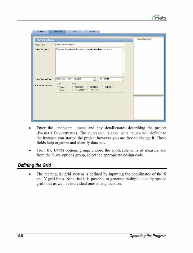
4-8 Operating the Program
• Enter the Project Name and any details/notes describing the project
(PROJECT DESCRIPTION). The Project Date And Time will default to the instance you started the project however you are free to change it. These fields help organize and identify data sets.
• From the UNITS options group, choose the applicable units of measure and from the CODE options group, select the appropriate design code.
Defining the Grid • The rectangular grid system is defined by inputting the coordinates of the X
and Y grid lines. Note that it is possible to generate multiple, equally spaced grid lines as well as individual ones at any location.

Operating the Program 4-9
• From the Define menu, choose Grid to have the program surface the GRID
folder as illustrated here…
• Alternatively, you could have clicked on the button located on the toolbar, and then
on the GRID tab.
• If you wish, you can enter a name and description for the grid. To do this, double-click on DESCRIPTION… found in the right item listing area. The program will surface the following dialog box…
• Enter a NAME and DESCRIPTION or note and click on OK.
To Enter Grid Lines Individually: • Double-click on SET UP… found in the right ITEM LISTING AREA to have the
program surface the following…
• Select the grid direction from the respective option group, X-Direction or Y-Direction. Grids in the X-Direction are perpendicular to the X-axis and those in the Y-Direction are perpendicular to the Y-axis.
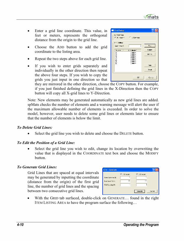
4-10 Operating the Program
• Enter a grid line coordinate. This value, in feet or meters, represents the orthogonal distance from the origin to the grid line.
• Choose the ADD button to add the grid coordinate to the listing area.
• Repeat the two steps above for each grid line.
• If you wish to enter grids separately and individually in the other direction then repeat the above four steps. If you wish to copy the grids you just input in one direction so that they are mirrored in the other direction, choose the COPY button. For example, if you just finished defining the grid lines in the X-Direction then the COPY button will copy all X-grid lines to Y-Direction.
Note: New elements may be generated automatically as new grid lines are added. spMats checks the number of elements and a warning message will alert the user if the maximum allowable number of elements is exceeded. In order to solve the model, however, user needs to delete some grid lines or elements later to ensure that the number of elements is below the limit.
To Delete Grid Lines: • Select the grid line you wish to delete and choose the DELETE button.
To Edit the Position of a Grid Line: • Select the grid line you wish to edit, change its location by overwriting the
value that is displayed in the COORDINATE text box and choose the MODIFY button.
To Generate Grid Lines: Grid Lines that are spaced at equal intervals may be generated by inputting the coordinate (distance from the origin) of the first grid line, the number of grid lines and the spacing between two consecutive grid lines.
• With the GRID tab surfaced, double-click on GENERATE… found in the right ITEM LISTING AREA to have the program surface the following…
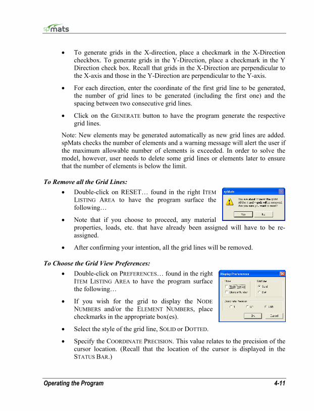
Operating the Program 4-11
• To generate grids in the X-direction, place a checkmark in the X-Direction checkbox. To generate grids in the Y-Direction, place a checkmark in the Y Direction check box. Recall that grids in the X-Direction are perpendicular to the X-axis and those in the Y-Direction are perpendicular to the Y-axis.
• For each direction, enter the coordinate of the first grid line to be generated, the number of grid lines to be generated (including the first one) and the spacing between two consecutive grid lines.
• Click on the GENERATE button to have the program generate the respective grid lines.
Note: New elements may be generated automatically as new grid lines are added. spMats checks the number of elements and a warning message will alert the user if the maximum allowable number of elements is exceeded. In order to solve the model, however, user needs to delete some grid lines or elements later to ensure that the number of elements is below the limit.
To Remove all the Grid Lines: • Double-click on RESET… found in the right ITEM
LISTING AREA to have the program surface the following…
• Note that if you choose to proceed, any material properties, loads, etc. that have already been assigned will have to be re-assigned.
• After confirming your intention, all the grid lines will be removed.
To Choose the Grid View Preferences: • Double-click on PREFERENCES… found in the right
ITEM LISTING AREA to have the program surface the following…
• If you wish for the grid to display the NODE NUMBERS and/or the ELEMENT NUMBERS, place checkmarks in the appropriate box(es).
• Select the style of the grid line, SOLID or DOTTED.
• Specify the COORDINATE PRECISION. This value relates to the precision of the cursor location. (Recall that the location of the cursor is displayed in the STATUS BAR.)
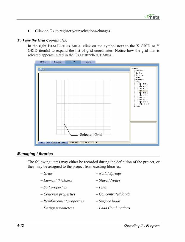
4-12 Operating the Program
• Click on OK to register your selections/changes.
To View the Grid Coordinates: In the right ITEM LISTING AREA, click on the symbol next to the X GRID or Y GRID item(s) to expand the list of grid coordinates. Notice how the grid that is selected appears in red in the GRAPHICS/INPUT AREA.
Managing Libraries The following items may either be recorded during the definition of the project, or they may be assigned to the project from existing libraries:
– Grids – Nodal Springs
– Element thickness – Slaved Nodes
– Soil properties – Piles
– Concrete properties – Concentrated loads
– Reinforcement properties – Surface loads
– Design parameters – Load Combinations
Selected Grid
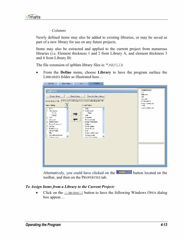
Operating the Program 4-13
– Columns
Newly defined items may also be added to existing libraries, or may be saved as part of a new library for use on any future projects.
Items may also be extracted and applied to the current project from numerous libraries (i.e. Element thickness 1 and 2 from Library A, and element thickness 3 and 4 from Library B)
The file extension of spMats library files is: *.MATLIB
• From the Define menu, choose Library to have the program surface the LIBRARIES folder as illustrated here…
Alternatively, you could have clicked on the button located on the toolbar, and then on the PROPERTIES tab.
To Assign Items from a Library to the Current Project: • Click on the button to have the following Windows OPEN dialog
box appear…

4-14 Operating the Program
• Locate the library file and click on OPEN to return focus to spMats. Notice how the contents of the selected library appear in the listing under “Current Library”…
• Click on the symbol next to various items to expand their contents. The items that will subsequently appear are items that have been pre-defined.
• Select the item and click on the arrow to copy the item and to
paste it into the current project. Any items copied over now become available for assigning.
• Repeat the above steps to select items from additional libraries.
To Create and Save a Library: • Click on the symbol next to the items appearing under the Current Project
listing to expand their contents.
• Locate the specific items defined in the current project and click on the
arrow to copy the item and to paste it into the current library.
• If there are items in the library that you would like to remove, simply highlight (click on) them and click on the icon
• To overwrite the library, click on the button. Any items copied over from the current project now become part of the saved library.
• To save the library as new, click on the button. Any items copied over from the current project now become part of the new library.

Operating the Program 4-15
Defining Material Properties Material properties such as:
• element thickness,
• soil modulus (Ks) and allowable pressure (Qa),
• concrete compressive strength ( 'cf ), unit weight (w), Young’s modulus (Ec),
and Poisson’s ratio (v),
• reinforcement yield strength (fy), Young’s modulus (Es), minimum reinforcement ratio and re-bar location,
• column type (round or rectangular) and dimensions, must be defined before they can be assigned to the elements on the grid.
• From the Define menu, choose Thickness, Concrete, Soil, Reinforcing Steel or Design Parameters to have the program surface the PROPERTIES folder as illustrated here…
Alternatively, you could have clicked on the button located on the toolbar, and then on the PROPERTIES tab.

4-16 Operating the Program
To define the Element Thickness • From the Define menu select Thickness, or if the PROPERTIES folder is
displayed, click on THICKNESS… found in the right ITEM LISTING AREA to have the program surface the Thickness input screen…
• Enter a thickness label or ID in the LABEL text box and enter the
corresponding thickness in the THICKNESS text box.
• Click on the ADD button to add the entry to the list box.
• Repeat the two steps above for each thickness entry.
• To edit an entry, select it from the list box, modify its value(s) in the text box(es) and click on the MODIFY button to register the changes.
• To delete a thickness entry, select it from the list box and click on the DELETE button.
To Define the Soil Properties: • From the Define menu select Soil, or if the PROPERTIES folder is displayed,
click on Soil… found in the right ITEM LISTING AREA to have the program surface the Soil input screen…
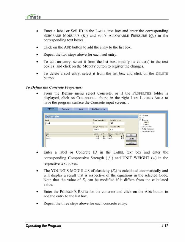
Operating the Program 4-17
• Enter a label or Soil ID in the LABEL text box and enter the corresponding SUBGRADE MODULUS (Ks) and soil’s ALLOWABLE PRESSURE (Qa) in the corresponding text boxes.
• Click on the ADD button to add the entry to the list box.
• Repeat the two steps above for each soil entry.
• To edit an entry, select it from the list box, modify its value(s) in the text box(es) and click on the MODIFY button to register the changes.
• To delete a soil entry, select it from the list box and click on the DELETE button.
To Define the Concrete Properties: • From the Define menu select Concrete, or if the PROPERTIES folder is
displayed, click on CONCRETE… found in the right ITEM LISTING AREA to have the program surface the Concrete input screen…
• Enter a label or Concrete ID in the LABEL text box and enter the
corresponding Compressive Strength ( 'cf ) and UNIT WEIGHT (w) in the
respective text boxes.
• The YOUNG’S MODULUS of elasticity (Ec) is calculated automatically and will display a result that is respective of the equations in the selected Code. Note that the value of Ec can be modified if it differs from the calculated value.
• Enter the POISSON’S RATIO for the concrete and click on the ADD button to add the entry to the list box.
• Repeat the three steps above for each concrete entry.

4-18 Operating the Program
• To edit an entry, select it from the list box, modify its value(s) in the text box(es) and click on the MODIFY button to register the changes.
• To delete a concrete material entry, select it from the list box and click on the DELETE button.
To Define the Reinforcing Steel Properties: • From the Define menu select Reinforcing Steel, or if the PROPERTIES folder
is displayed, click on REINFORCEMENT… found in the right ITEM LISTING AREA to have the program surface the Reinforcement input screen…
• Enter a label or Reinforcement ID in the LABEL text box and enter the
corresponding Yield Strength (fy) and the YOUNG’S MODULUS of elasticity (Es) for the steel.
• Click on the ADD button to add the entry to the list box.
• Repeat the two steps above for each reinforcement entry.
• To edit an entry, select it from the list box, modify its value(s) in the text box(es) and click on the MODIFY button to register the changes.
• To delete a reinforcement material entry, select it from the list box and click on the DELETE button.
To Define the Design Parameters: • From the Define menu select Design Parameters, or if the PROPERTIES folder
is displayed, click on DESIGN PARAMETERS… found in the right ITEM LISTING AREA to have the program surface the Design Parameters input screen.
• Enter a label or ID in the LABEL text box and enter the corresponding MINIMUM REINFORCEMENT RATIO as a percentage of the gross area.
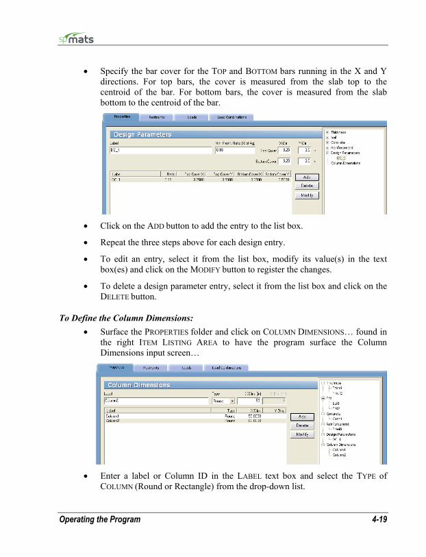
Operating the Program 4-19
• Specify the bar cover for the TOP and BOTTOM bars running in the X and Y directions. For top bars, the cover is measured from the slab top to the centroid of the bar. For bottom bars, the cover is measured from the slab bottom to the centroid of the bar.
• Click on the ADD button to add the entry to the list box.
• Repeat the three steps above for each design entry.
• To edit an entry, select it from the list box, modify its value(s) in the text box(es) and click on the MODIFY button to register the changes.
• To delete a design parameter entry, select it from the list box and click on the DELETE button.
To Define the Column Dimensions: • Surface the PROPERTIES folder and click on COLUMN DIMENSIONS… found in
the right ITEM LISTING AREA to have the program surface the Column Dimensions input screen…
• Enter a label or Column ID in the LABEL text box and select the TYPE of
COLUMN (Round or Rectangle) from the drop-down list.
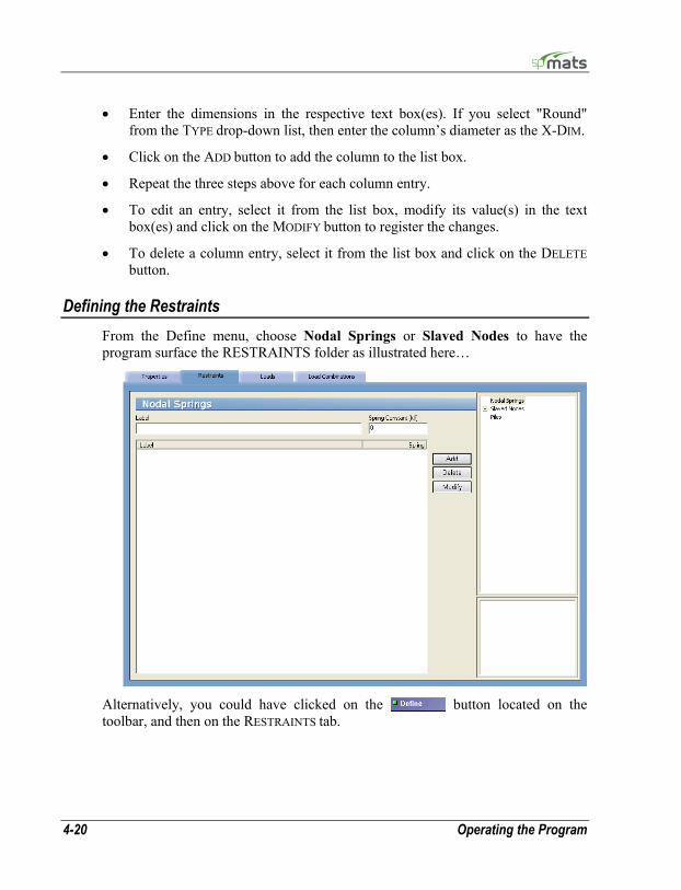
4-20 Operating the Program
• Enter the dimensions in the respective text box(es). If you select "Round" from the TYPE drop-down list, then enter the column’s diameter as the X-DIM.
• Click on the ADD button to add the column to the list box.
• Repeat the three steps above for each column entry.
• To edit an entry, select it from the list box, modify its value(s) in the text box(es) and click on the MODIFY button to register the changes.
• To delete a column entry, select it from the list box and click on the DELETE button.
Defining the Restraints From the Define menu, choose Nodal Springs or Slaved Nodes to have the program surface the RESTRAINTS folder as illustrated here…
Alternatively, you could have clicked on the button located on the toolbar, and then on the RESTRAINTS tab.
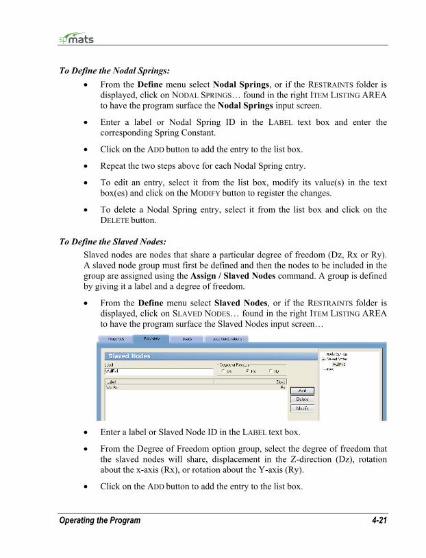
Operating the Program 4-21
To Define the Nodal Springs: • From the Define menu select Nodal Springs, or if the RESTRAINTS folder is
displayed, click on NODAL SPRINGS… found in the right ITEM LISTING AREA to have the program surface the Nodal Springs input screen.
• Enter a label or Nodal Spring ID in the LABEL text box and enter the corresponding Spring Constant.
• Click on the ADD button to add the entry to the list box.
• Repeat the two steps above for each Nodal Spring entry.
• To edit an entry, select it from the list box, modify its value(s) in the text box(es) and click on the MODIFY button to register the changes.
• To delete a Nodal Spring entry, select it from the list box and click on the DELETE button.
To Define the Slaved Nodes: Slaved nodes are nodes that share a particular degree of freedom (Dz, Rx or Ry). A slaved node group must first be defined and then the nodes to be included in the group are assigned using the Assign / Slaved Nodes command. A group is defined by giving it a label and a degree of freedom.
• From the Define menu select Slaved Nodes, or if the RESTRAINTS folder is displayed, click on SLAVED NODES… found in the right ITEM LISTING AREA to have the program surface the Slaved Nodes input screen…
• Enter a label or Slaved Node ID in the LABEL text box.
• From the Degree of Freedom option group, select the degree of freedom that the slaved nodes will share, displacement in the Z-direction (Dz), rotation about the x-axis (Rx), or rotation about the Y-axis (Ry).
• Click on the ADD button to add the entry to the list box.
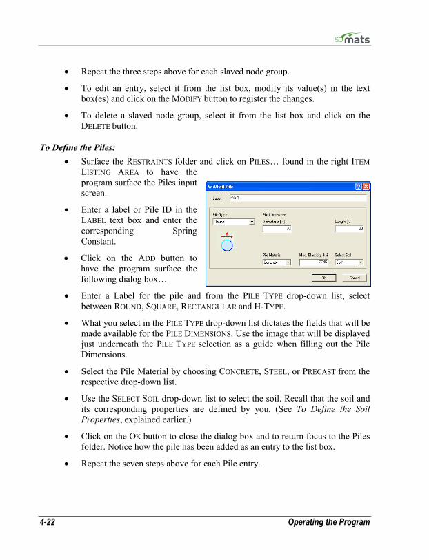
4-22 Operating the Program
• Repeat the three steps above for each slaved node group.
• To edit an entry, select it from the list box, modify its value(s) in the text box(es) and click on the MODIFY button to register the changes.
• To delete a slaved node group, select it from the list box and click on the DELETE button.
To Define the Piles: • Surface the RESTRAINTS folder and click on PILES… found in the right ITEM
LISTING AREA to have the program surface the Piles input screen.
• Enter a label or Pile ID in the LABEL text box and enter the corresponding Spring Constant.
• Click on the ADD button to have the program surface the following dialog box…
• Enter a Label for the pile and from the PILE TYPE drop-down list, select between ROUND, SQUARE, RECTANGULAR and H-TYPE.
• What you select in the PILE TYPE drop-down list dictates the fields that will be made available for the PILE DIMENSIONS. Use the image that will be displayed just underneath the PILE TYPE selection as a guide when filling out the Pile Dimensions.
• Select the Pile Material by choosing CONCRETE, STEEL, or PRECAST from the respective drop-down list.
• Use the SELECT SOIL drop-down list to select the soil. Recall that the soil and its corresponding properties are defined by you. (See To Define the Soil Properties, explained earlier.)
• Click on the OK button to close the dialog box and to return focus to the Piles folder. Notice how the pile has been added as an entry to the list box.
• Repeat the seven steps above for each Pile entry.

Operating the Program 4-23
• To edit an entry, select it from the list box, if you wish to modify it’s LABEL or SPRING CONSTANT, simply edit the values in the respective text boxes and click on the MODIFY button to register the changes. If you wish to edit the TYPE, DIMENSIONS, SOIL TYPE, or PILE MATERIAL, click on the EDIT button to surface the corresponding dialog box, modify the value(s) in the text box(es) and then g click on the OK button to close the dialog box and to return focus to the Piles folder.
• To delete a Pile entry, select it from the list box and click on the DELETE button.
Defining the Loads Nodal and element loads are defined using the Define / Loads command. They are then assigned to the nodes using the Assign / Nodal Loads command, and to elements using the Assign / Surface Loads command.
• From the Define menu, choose Loads to have the program surface the LOADS folder.
Alternatively, you could have clicked on the button located on the toolbar, and then on the LOADS tab.
To Define the Concentrated Load(s): • Surface the LOADS folder and click on CONCENTRATED… found in the right
ITEM LISTING AREA to have the program surface the Concentrated Loads input screen…
• Enter a label or Concentrated Load ID in the LABEL text box.
• From the Case drop-down list, select a load case (A through F). Note that loads defined under a particular load case may be applied to the slab under that load case only.
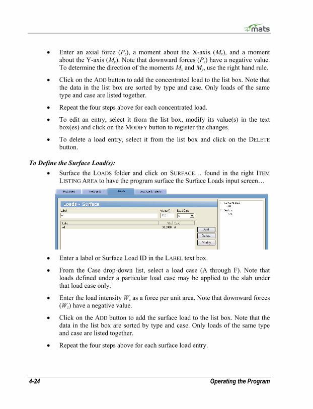
4-24 Operating the Program
• Enter an axial force (Pz), a moment about the X-axis (Mx), and a moment about the Y-axis (My). Note that downward forces (Pz) have a negative value. To determine the direction of the moments Mx and My, use the right hand rule.
• Click on the ADD button to add the concentrated load to the list box. Note that the data in the list box are sorted by type and case. Only loads of the same type and case are listed together.
• Repeat the four steps above for each concentrated load.
• To edit an entry, select it from the list box, modify its value(s) in the text box(es) and click on the MODIFY button to register the changes.
• To delete a load entry, select it from the list box and click on the DELETE button.
To Define the Surface Load(s): • Surface the LOADS folder and click on SURFACE… found in the right ITEM
LISTING AREA to have the program surface the Surface Loads input screen…
• Enter a label or Surface Load ID in the LABEL text box.
• From the Case drop-down list, select a load case (A through F). Note that loads defined under a particular load case may be applied to the slab under that load case only.
• Enter the load intensity Wz as a force per unit area. Note that downward forces (Wz) have a negative value.
• Click on the ADD button to add the surface load to the list box. Note that the data in the list box are sorted by type and case. Only loads of the same type and case are listed together.
• Repeat the four steps above for each surface load entry.
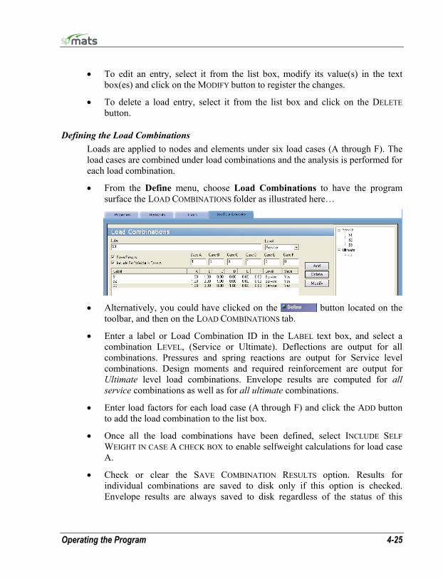
Operating the Program 4-25
• To edit an entry, select it from the list box, modify its value(s) in the text box(es) and click on the MODIFY button to register the changes.
• To delete a load entry, select it from the list box and click on the DELETE button.
Defining the Load Combinations Loads are applied to nodes and elements under six load cases (A through F). The load cases are combined under load combinations and the analysis is performed for each load combination.
• From the Define menu, choose Load Combinations to have the program surface the LOAD COMBINATIONS folder as illustrated here…
• Alternatively, you could have clicked on the button located on the
toolbar, and then on the LOAD COMBINATIONS tab.
• Enter a label or Load Combination ID in the LABEL text box, and select a combination LEVEL, (Service or Ultimate). Deflections are output for all combinations. Pressures and spring reactions are output for Service level combinations. Design moments and required reinforcement are output for Ultimate level load combinations. Envelope results are computed for all service combinations as well as for all ultimate combinations.
• Enter load factors for each load case (A through F) and click the ADD button to add the load combination to the list box.
• Once all the load combinations have been defined, select INCLUDE SELF WEIGHT IN CASE A CHECK BOX to enable selfweight calculations for load case A.
• Check or clear the SAVE COMBINATION RESULTS option. Results for individual combinations are saved to disk only if this option is checked. Envelope results are always saved to disk regardless of the status of this

4-26 Operating the Program
option. Check or clear the INCLUDE SELF-WEIGHT IN CASE A option. If this option is checked, the self-weight of the slab will be automatically computed and included under load case A.
• Repeat the four steps above for each load combination entry.
• To edit an entry, select it from the list box, modify its value(s) in the text box(es) and click on the MODIFY button to register the changes.
• To delete a load combination, select it from the list box and click on the DELETE button.
Assigning the material properties Once the grid, all components, material properties, design parameters, loads and load combinations have been defined, you are ready to start assigning them - thereby putting the project together.
• From the Assign menu, choose Thickness, Concrete, Soil, Reinforcing Steel or Design Parameters to have the program surface the PROPERTIES folder as illustrated here…

Operating the Program 4-27
Alternatively, you could have clicked on the button located on the toolbar, and then on the PROPERTIES tab.
To Assign the Element Thickness: • From the Assign menu, choose Thickness, or if the PROPERTIES folder is
displayed, click on the symbol next to THICKNESS… found in the right ITEM LISTING AREA to expand the THICKNESS list. The thicknesses that will appear are those defined using the Define / Thickness command. See To Define The Element Thickness.
• Select the thickness to be assigned. This becomes the active assignment. By default, the program will display all elements that share the active assignment in red and the inactive assignment in cyan. Unassigned grid space is by default displayed in white. Recall however that you may change the color preferences to your liking with the Options / Display command.
• In the GRAPHICS AREA, using the left-mouse button, marquee select a grid space or a group of grid spaces (or click a single grid space). The selected grid spaces are shown in red or in the color specified for ACTIVE OBJECTS in the DISPLAY folder.
• To delete an element, remove its thickness assignment. To do so, repeat the step above using instead, the right mouse button.
• Repeat the three steps above for each thickness entry.
To Assign the Soil Properties: • From the Assign menu select Soil, or if the PROPERTIES folder is displayed,
click on the symbol next to SOIL… found in the right ITEM LISTING AREA to expand the SOIL list. The soils that will appear are those defined using the Define / Soil command. See To Define The Soil Properties.
• Select the soil to be assigned. This becomes the active assignment. By default, the program will display all elements that share the active assignment in red and the inactive assignment in cyan. Unassigned elements are by default displayed in powder blue. Recall however that you may change the color preferences to your liking with the Options / Display command.
• In the GRAPHICS AREA, using the left-mouse button, marquee select an element or a group of elements (or click a single element). The selected elements are shown in red or in the color specified for ACTIVE OBJECTS in the DISPLAY folder.
4-28 Operating the Program
• To remove a soil assignment, repeat the step above using instead, the right mouse button.
• Repeat the three steps above for each soil entry.
To Assign the Concrete Properties: • From the Assign menu select Concrete, or if the PROPERTIES folder is
displayed, click on the symbol next to CONCRETE… found in the right ITEM LISTING AREA to expand the CONCRETE list. The concrete that will appear are those defined using the Define / Concrete command. See To Define The Concrete Properties.
• Select the concrete to be assigned. This becomes the active assignment. By default, the program will display all elements that share the active assignment in red and the inactive assignment in cyan. Unassigned elements are by default displayed in powder blue. Recall however that you may change the color preferences to your liking with the Options / Display command.
• In the GRAPHICS AREA, using the left-mouse button, marquee select an element or a group of elements (or click a single element). The selected elements are shown in red or in the color specified for ACTIVE OBJECTS in the DISPLAY folder.
• To remove a concrete assignment, repeat the step above using instead, the right mouse button.
• Repeat the three steps above for each concrete entry.
To Assign the Reinforcing Steel Properties: • From the Assign menu select Reinforcing Steel, or if the PROPERTIES folder
is displayed, click on the symbol next to REINFORCING STEEL… found in the right ITEM LISTING AREA to expand the REINFORCING STEEL list. The reinforcing steel entries that will appear are those defined using the Define/Reinforcing Steel command. See To Define The Reinforcing Steel Properties.
• Select the reinforcing steel to be assigned. This becomes the active assignment. By default, the program will display all elements that share the active assignment in red and the inactive assignment in cyan. Unassigned elements are by default displayed in powder blue. Recall however that you may change the color preferences to your liking with the Options / Display command.

Operating the Program 4-29
• In the GRAPHICS AREA, using the left-mouse button, marquee select an element or a group of elements (or click a single element). The selected elements are shown in red or in the color specified for ACTIVE OBJECTS in the DISPLAY folder.
• To remove a reinforcing steel assignment, repeat the step above using instead, the right mouse button.
• Repeat the three steps above for each reinforcing steel entry.
To Assign Design Parameters: • From the Assign menu select Design Parameters, or if the PROPERTIES folder
is displayed, click on the symbol next to DESIGN PARAMETERS… found in the right ITEM LISTING AREA to expand the DESIGN PARAMETERS list. The design parameters that will appear are those defined using the Define / Design Parameters command. See To Define The Design Parameters.
• Select the design parameter entry to be assigned. This becomes the active assignment. By default, the program will display all elements that share the active assignment in red and the inactive assignment in cyan. Unassigned elements are by default displayed in powder blue. Recall however that you may change the color preferences to your liking with the Options / Display command.
• In the GRAPHICS AREA, using the left-mouse button, marquee select an element or a group of elements (or click a single element). The selected elements are shown in red or in the color specified for ACTIVE OBJECTS in the DISPLAY folder.
• To remove a design parameter assignment, repeat the step above using instead, the right mouse button.
• Repeat the three steps above for each design parameter entry.

4-30 Operating the Program
To Assign the Columns:
• From the Assign menu select Column Dimensions, or if the PROPERTIES
folder is displayed, click on the symbol next to COLUMN DIMENSIONS… found in the right ITEM LISTING AREA to expand the COLUMN DIMENSIONS list.
• Select the column entry to be assigned. This becomes the active assignment. By default, the program will display all nodes that share the active assignment in red and nodes with a different assignment in cyan. Recall however that you may change the color preferences to your liking with the Options / Display command.
• In the GRAPHICS AREA, using the left-mouse button, marquee select a node or a group of nodes (or click a single node). Columns are shown to scale at the selected nodes in red or in the color specified for ACTIVE OBJECTS in the DISPLAY folder.
• To remove a column assignment, repeat the step above using instead, the right mouse button.
• Repeat the three steps above for each column entry.

Operating the Program 4-31
Assigning the Restraints Once the grid, all components, material properties, design parameters, loads and load combinations have been defined, you are ready to start assigning them - thereby putting the project together.
• From the Assign menu, choose Nodal Springs, Slaved Nodes or Restraints
to have the program surface the RESTRAINTS folder as illustrated above…
Alternatively, you could have clicked on the button located on the toolbar, and then on the RESTRAINTS tab.
To Assign Nodal Restraints: Fixed nodes or supports are assigned using the Assign / Restraints command.
• From the Assign menu select Restraints, or if the RESTRAINTS is displayed, click on the symbol next to RESTRAINTS… found in the right ITEM LISTING AREA to expand the RESTRAINTS list. You will be able to restrain Dz, Rx and Ry degrees of freedom.
4-32 Operating the Program
• Select the nodal restraint to be assigned. This becomes the active assignment. By default, the program will display all nodes that share the active assignment in red and nodes with a different assignment in cyan. Recall however that you may change the color preferences to your liking with the Options / Display command.
• In the GRAPHICS AREA, using the left-mouse button, marquee select a node or a group of nodes (or click a single node). The selected nodes are shown in red or in the color specified for ACTIVE OBJECTS in the DISPLAY folder.
• To remove a nodal restraint assignment, repeat the step above using instead, the right mouse button.
• Repeat the three steps above for each degree of freedom.
To Assign Nodal Springs: • From the Assign menu select Nodal Springs, or if the RESTRAINTS folder is
displayed, click on the symbol next to NODAL SPRINGS… found in the right ITEM LISTING AREA to expand the NODAL SPRINGS list. The nodal springs that appear are those defined using the Define/Nodal Springs command. See To Define The Nodal Springs.
• Select the nodal spring to be assigned. This becomes the active assignment. By default, the program will display all nodes that share the active assignment in red and nodes with a different assignment in cyan. Recall however that you may change the color preferences to your liking with the Options / Display command. See To Change The Font and Color Preferences.
• In the GRAPHICS AREA, using the left-mouse button, marquee select a node or a group of nodes (or click a single node). The selected nodes are shown in red or in the color specified for ACTIVE OBJECTS in the DISPLAY folder.
• To remove a nodal spring assignment, repeat the step above using instead, the right mouse button.
• Repeat the three steps above for each nodal spring entry.
To Assign Slaved Nodes: • From the Assign menu select Slaved Nodes, or if the RESTRAINTS folder is
displayed, click on the symbol next to SLAVED NODES… found in the right ITEM LISTING AREA to expand the SLAVED NODES list. The slaved node
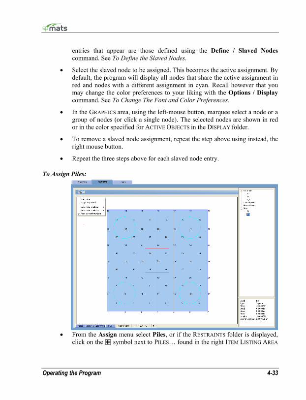
Operating the Program 4-33
entries that appear are those defined using the Define / Slaved Nodes command. See To Define the Slaved Nodes.
• Select the slaved node to be assigned. This becomes the active assignment. By default, the program will display all nodes that share the active assignment in red and nodes with a different assignment in cyan. Recall however that you may change the color preferences to your liking with the Options / Display command. See To Change The Font and Color Preferences.
• In the GRAPHICS area, using the left-mouse button, marquee select a node or a group of nodes (or click a single node). The selected nodes are shown in red or in the color specified for ACTIVE OBJECTS in the DISPLAY folder.
• To remove a slaved node assignment, repeat the step above using instead, the right mouse button.
• Repeat the three steps above for each slaved node entry.
To Assign Piles:
• From the Assign menu select Piles, or if the RESTRAINTS folder is displayed,
click on the symbol next to PILES… found in the right ITEM LISTING AREA
4-34 Operating the Program
to expand the PILES list. The piles that appear are those previously defined by you. See To Define the Piles.
• Select the pile to be assigned. This becomes the active assignment. By default, the program will display all nodes that share the active assignment in red and nodes with a different assignment in cyan. Recall however that you may change the color preferences to your liking with the Options / Display command. See To Change The Font and Color Preferences.
• In the GRAPHICS AREA, using the left-mouse button, marquee select a node or a group of nodes (or click a single node). Piles are shown to scale at the selected nodes in red or in the color specified for ACTIVE OBJECTS in the DISPLAY folder.
• To remove a pile assignment, repeat the step above using instead, the right mouse button.
• Repeat the three steps above for each pile in the ITEM LISTING AREA.
Applying the Loads Once the grid, all components, material properties, design parameters, loads and load combinations have been defined, you are ready to start assigning them - thereby putting the project together.
• From the Assign menu, choose Surface Loads or Nodal Loads to have the program surface the LOADS folder as illustrated below
Alternatively, you could have clicked on the button located on the toolbar, and then on the LOADS tab. If columns or piles have been assigned to the model, they are displayed in the color specified for COLUMN or PILES in the DISPLAY SETTINGS. If it is preferred not to show columns or piles, right click on empty space on the view window, and then uncheck Show Columns or Show Piles on the pop-up menu.
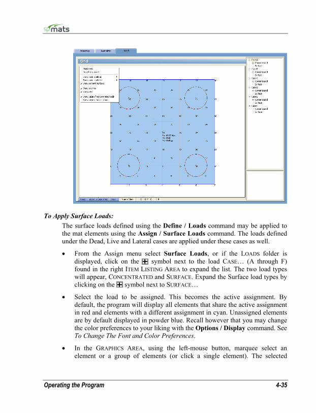
Operating the Program 4-35
To Apply Surface Loads: The surface loads defined using the Define / Loads command may be applied to the mat elements using the Assign / Surface Loads command. The loads defined under the Dead, Live and Lateral cases are applied under these cases as well.
• From the Assign menu select Surface Loads, or if the LOADS folder is displayed, click on the symbol next to the load CASE… (A through F) found in the right ITEM LISTING AREA to expand the list. The two load types will appear, CONCENTRATED and SURFACE. Expand the Surface load types by clicking on the symbol next to SURFACE…
• Select the load to be assigned. This becomes the active assignment. By default, the program will display all elements that share the active assignment in red and elements with a different assignment in cyan. Unassigned elements are by default displayed in powder blue. Recall however that you may change the color preferences to your liking with the Options / Display command. See To Change The Font and Color Preferences.
• In the GRAPHICS AREA, using the left-mouse button, marquee select an element or a group of elements (or click a single element). The selected
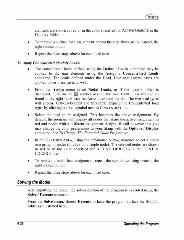
4-36 Operating the Program
elements are shown in red or in the color specified for ACTIVE OBJECTS in the DISPLAY folder.
• To remove a surface load assignment, repeat the step above using instead, the right mouse button.
• Repeat the three steps above for each load case.
To Apply Concentrated (Nodal) Loads: • The concentrated loads defined using the Define / Loads command may be
applied to the mat elements using the Assign / Concentrated Loads command. The loads defined under the Dead, Live and Lateral cases are applied under these cases as well.
• From the Assign menu select Nodal Loads, or if the LOADS folder is displayed, click on the symbol next to the load CASE… (A through F) found in the right ITEM LISTING AREA to expand the list. The two load types will appear, CONCENTRATED and SURFACE. Expand the Concentrated load types by clicking on the symbol next to CONCENTRATED…
• Select the load to be assigned. This becomes the active assignment. By default, the program will display all nodes that share the active assignment in red and nodes with a different assignment in cyan. Recall however that you may change the color preferences to your liking with the Options / Display command. See To Change The Font and Color Preferences.
• In the GRAPHICS AREA, using the left-mouse button, marquee select a nodes or a group of nodes (or click on a single node). The selected nodes are shown in red or in the color specified for ACTIVE OBJECTS in the FONT & COLOR folder.
• To remove a nodal load assignment, repeat the step above using instead, the right mouse button.
• Repeat the three steps above for each load case.
Solving the Model After inputting the model, the solver portion of the program is executed using the Solve / Execute command.
From the Solve menu, choose Execute to have the program surface the SOLVER folder as illustrated here…
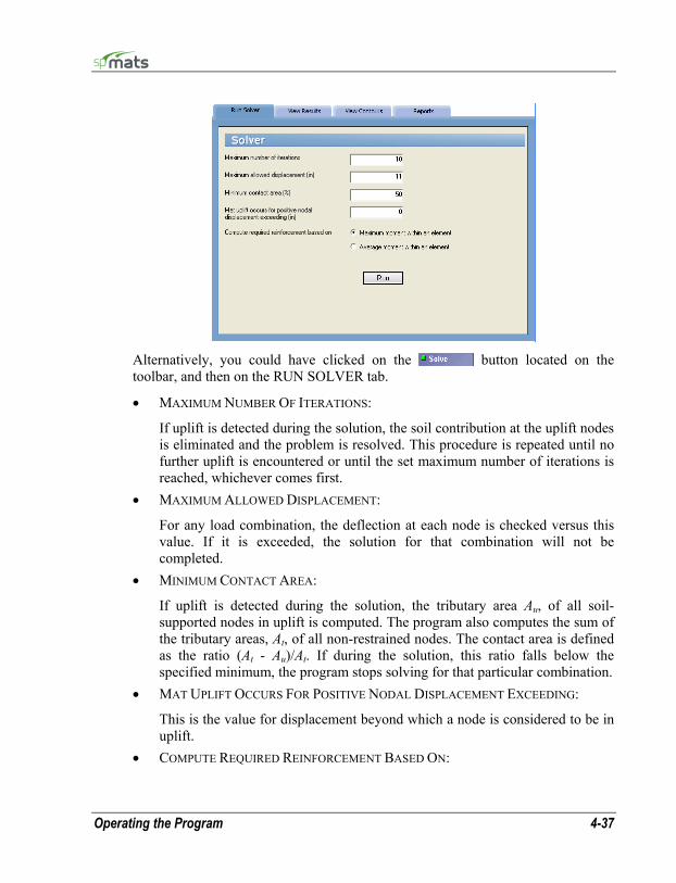
Operating the Program 4-37
Alternatively, you could have clicked on the button located on the toolbar, and then on the RUN SOLVER tab.
• MAXIMUM NUMBER OF ITERATIONS:
If uplift is detected during the solution, the soil contribution at the uplift nodes is eliminated and the problem is resolved. This procedure is repeated until no further uplift is encountered or until the set maximum number of iterations is reached, whichever comes first.
• MAXIMUM ALLOWED DISPLACEMENT:
For any load combination, the deflection at each node is checked versus this value. If it is exceeded, the solution for that combination will not be completed.
• MINIMUM CONTACT AREA:
If uplift is detected during the solution, the tributary area Au, of all soil-supported nodes in uplift is computed. The program also computes the sum of the tributary areas, At, of all non-restrained nodes. The contact area is defined as the ratio (At - Au)/At. If during the solution, this ratio falls below the specified minimum, the program stops solving for that particular combination.
• MAT UPLIFT OCCURS FOR POSITIVE NODAL DISPLACEMENT EXCEEDING:
This is the value for displacement beyond which a node is considered to be in uplift.
• COMPUTE REQUIRED REINFORCEMENT BASED ON:
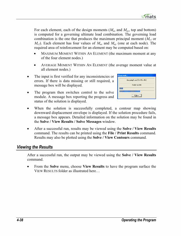
4-38 Operating the Program
For each element, each of the design moments (Mux and Muy, top and bottom) is computed for a governing ultimate load combination. The governing load combination is the one that produces the maximum principal moment (Mr1 or Mr2). Each element has four values of Mux and Muy (one at each node). The required area of reinforcement for an element may be computed based on: • MAXIMUM MOMENT WITHIN AN ELEMENT (the maximum moment at any
of the four element nodes.)
• AVERAGE MOMENT WITHIN AN ELEMENT (the average moment value at all element nodes.)
• The input is first verified for any inconsistencies or errors. If there is data missing or still required, a message box will be displayed.
• The program then switches control to the solve module. A message box reporting the progress and status of the solution is displayed.
• When the solution is successfully completed, a contour map showing downward displacement envelope is displayed. If the solution procedure fails, a message box appears. Detailed information on the solution may be found in the Solve / View Results / Solve Messages window.
• After a successful run, results may be viewed using the Solve / View Results command. The results can be printed using the File / Print Results command. Results may also be plotted using the Solve / View Contours command.
Viewing the Results After a successful run, the output may be viewed using the Solve / View Results command.
• From the Solve menu, choose View Results to have the program surface the VIEW RESULTS folder as illustrated here…
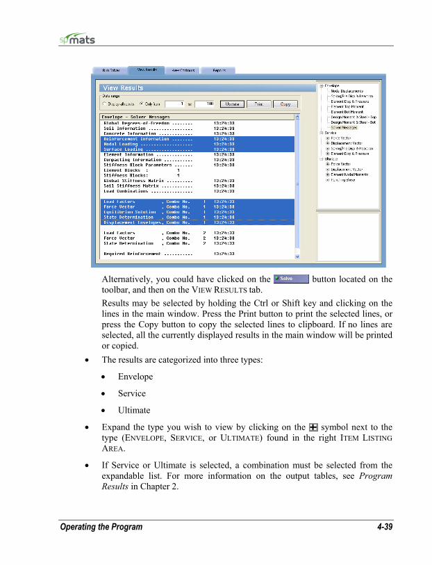
Operating the Program 4-39
Alternatively, you could have clicked on the button located on the toolbar, and then on the VIEW RESULTS tab. Results may be selected by holding the Ctrl or Shift key and clicking on the lines in the main window. Press the Print button to print the selected lines, or press the Copy button to copy the selected lines to clipboard. If no lines are selected, all the currently displayed results in the main window will be printed or copied.
• The results are categorized into three types:
• Envelope
• Service
• Ultimate
• Expand the type you wish to view by clicking on the symbol next to the type (ENVELOPE, SERVICE, or ULTIMATE) found in the right ITEM LISTING AREA.
• If Service or Ultimate is selected, a combination must be selected from the expandable list. For more information on the output tables, see Program Results in Chapter 2.
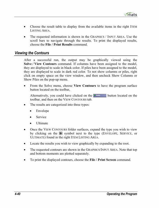
4-40 Operating the Program
• Choose the result table to display from the available items in the right ITEM LISTING AREA.
• The requested information is shown in the GRAPHICS / INPUT AREA. Use the scroll bars to navigate through the results. To print the displayed results, choose the File / Print Results command.
Viewing the Contours After a successful run, the output may be graphically viewed using the Solve / View Contours command. If columns have been assigned to the model, they are displayed to scale in black color. If piles have been assigned to the model, they are displayed to scale in dark red color. To not show columns or piles, right click on empty space on the view window, and then uncheck Show Columns or Show Piles on the pop-up menu.
• From the Solve menu, choose View Contours to have the program surface button located on the toolbar,
Alternatively, you could have clicked on the button located on the toolbar, and then on the VIEW CONTOURS tab.
• The results are categorized into three types:
• Envelope
• Service
• Ultimate
• Once the VIEW CONTOURS folder surfaces, expand the type you wish to view by clicking on the symbol next to the type (ENVELOPE, SERVICE, or ULTIMATE) found in the right ITEM LISTING AREA.
• Locate the results you wish to view graphically by expanding to the root.
• The requested contours are shown in the GRAPHICS/INPUT AREA. Note that top and bottom moments are plotted separately.
• To print the displayed contours, choose the File / Print Screen command.
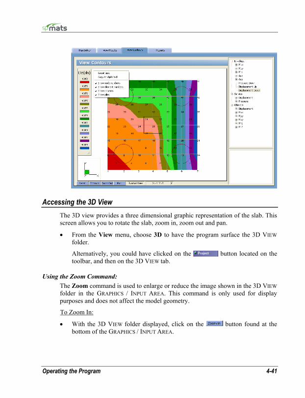
Operating the Program 4-41
Accessing the 3D View The 3D view provides a three dimensional graphic representation of the slab. This screen allows you to rotate the slab, zoom in, zoom out and pan.
• From the View menu, choose 3D to have the program surface the 3D VIEW folder.
Alternatively, you could have clicked on the button located on the toolbar, and then on the 3D VIEW tab.
Using the Zoom Command: The Zoom command is used to enlarge or reduce the image shown in the 3D VIEW folder in the GRAPHICS / INPUT AREA. This command is only used for display purposes and does not affect the model geometry.
To Zoom In:
• With the 3D VIEW folder displayed, click on the button found at the bottom of the GRAPHICS / INPUT AREA.
4-42 Operating the Program
• Using the left-mouse button, marquee select the portion of the graphical image you wish to enlarge. The selected area is enlarged to occupy the entire GRAPHICS / INPUT area.
To Zoom Out:
• With the 3D VIEW displayed, click on the button found at the bottom of the GRAPHICS / INPUT AREA.
• Using the left-mouse button, marquee select the portion of the graphical image you wish to reduce. The selected area is proportionally readjusted in the GRAPHICS / INPUT area.
Using the Pan Command: The Pan command is used to move the image shown in the 3D VIEW folder in the GRAPHICS / INPUT area. Image panning or translation is a linear movement of the viewport. This command is only used for display purposes and does not affect the model geometry.
• With the 3D VIEW folder displayed, click on the button found at the bottom of the GRAPHICS / INPUT area.
Operating the Program 4-43
• Click and hold the left-mouse button on the graphic while dragging it around the GRAPHICS / INPUT area. The image is anchored (moved) when the left-mouse button is released.
Using the Reset Command: The Reset command is used to reset the image shown in the 3D VIEW folder in the GRAPHICS / INPUT AREA to its default position.
• With the 3D VIEW folder displayed, click on the button found at the bottom of the GRAPHICS / INPUT area.
Alternatively, you could simply right-button click anywhere within the GRAPHICS / INPUT area.
Using the Rotate Command: The Rotate command is used (in isometric 3D only) to rotate the image shown in the 3D VIEW folder so that the model may be viewed from a different viewpoint. This command works with the axis-orientation box located at the bottom of the GRAPHICS / INPUT area…
This command is only used for display purposes and does not affect the model geometry.
• With the 3D VIEW folder displayed, click and hold down the left mouse button on the axis-orientation box.
• Drag the mouse in any direction while holding down the left-mouse button. Notice the corresponding rotations of both the axis bar as well as the graphic. The axis orientation represents the position of the model as soon as the left-mouse button is released.
Defining the Options There are many options that can be set as default so that they are saved in memory to be applied to any subsequent project until they are changed again.
From the Options menu, choose Startup Defaults, Autosave, Display or Statistics to have the program surface the respective OPTION folder as illustrated.
Alternatively, you could have clicked on the button located on the toolbar.

4-44 Operating the Program
To Define the Startup Defaults: The Options / Startup Defaults command is used to save the current file settings to be used in future input sessions. Default settings are saved in the Windows registry file. Settings that are saved include units of measure, code, and default directories.
• With the STARTUP folder surfaced, from the UNITS options group, choose the applicable units of measure and from the CODE options group, select the appropriate design code.
• Specify a default data directory. The path you specify here is where any data files you save will be saved by default. Note, however, that you will still be able to specify a different location when you attempt to save. See Saving the Data.
• You may also control the number of lines printed per page.
To Control the Autosave feature: The Options / Autosave command is used to force the program to save your input data to disk at predefined intervals. This minimizes loss of data in case of a power loss or computer lock-up. Note that the file must be named (using the File / Save As command) prior to activating this feature.
• With the AUTOSAVE folder surfaced, place a checkmark in the ENABLE AUTOSAVE box to activate the auto save feature.
• In the Frequency text box, specify the time interval that you would like the program to run the autosave feature.

Operating the Program 4-45
To Customize Display settings: The Display command is used to change various display settings such as font, object colors, 3D View options and 2D View options
• Within the FONT group, click on the CHOOSE FONT button to select the font type and size that will be used in plotting the node and element numbers on the graphical display. The font types that appear in the list are those saved in your WINDOWS/FONTS directory. The font you specify here is also used in screen-printing.
• Use the color drop-down lists within the OBJECT COLORS group to select preferred colors for the following…
• Grid
• Active object
• Inactive object
• Frame
• Background
• Column
• Pile
• Nodal Load
• Surface Load
• Settings within the 3D VIEW OPTIONS group control the 3D display of the
model. The user can modify the following …
• VERTICAL SCALE – to change scaling along the Z (vertical) axis of the model
• Angle XY – to change the angle at which the model is viewed with respect to the Z (vertical axis) of the screen
• Angle YZ – to change the angle at which the model is viewed with respect to the X (horizontal axis) of the screen

4-46 Operating the Program
• Settings within the 2D VIEW OPTIONS group control the display of the model in 2D view windows such as GRID, ASSIGN, and CONTOUR windows. The user can modify the following …
• SHOW NODE LABELS AS: numbers or coordinates
• SHOW NODE LABELS FOR: nodes with assigned loads, piles, restraints, columns or all nodes
• SHOW ELEMENT NUMBERS – toggles the display of element numbers
• SHOW COLUMNS – toggles the display of column locations, column sections are displayed to scale
• SHOW PILES – toggles the display of pile locations, pile sections are displayed to scale
• GRID LINE TYPE – selects the style of the grid line, SOLID or DOTTED
• COORDINATE PRECISION – specifies the precision of the cursor location displayed in the STATUS BAR.
To View the Project Statistics: • Surface the STATISTICS folder by
using the Options / Statistics command…
Alternatively, you could have clicked on the button located on the toolbar, and then on the STATISTICS tab.
• The folder displays a statistical summary on the number of nodes, elements and definitions.
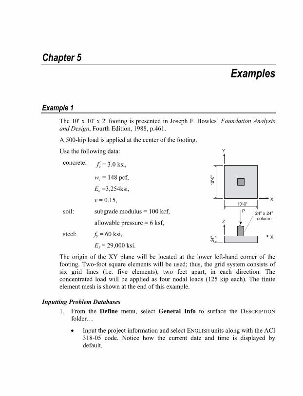
Chapter 5 Examples
Example 1 The 10' x 10' x 2' footing is presented in Joseph F. Bowles’ Foundation Analysis and Design, Fourth Edition, 1988, p.461.
A 500-kip load is applied at the center of the footing.
Use the following data:
concrete: 'cf = 3.0 ksi,
wc = 148 pcf,
Ec =3,254ksi,
v = 0.15,
soil: subgrade modulus = 100 kcf,
allowable pressure = 6 ksf,
steel: fy = 60 ksi,
Es = 29,000 ksi.
The origin of the XY plane will be located at the lower left-hand corner of the footing. Two-foot square elements will be used; thus, the grid system consists of six grid lines (i.e. five elements), two feet apart, in each direction. The concentrated load will be applied as four nodal loads (125 kip each). The finite element mesh is shown at the end of this example.
Inputting Problem Databases 1. From the Define menu, select General Info to surface the DESCRIPTION
folder…
• Input the project information and select ENGLISH units along with the ACI 318-05 code. Notice how the current date and time is displayed by default.
24” x 24”column
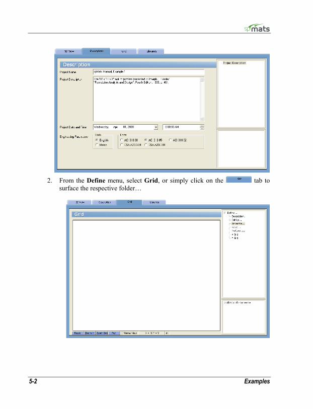
5-2 Examples
2. From the Define menu, select Grid, or simply click on the tab to
surface the respective folder…

Examples 5-3
Since the grid layout is uniform, and symmetrical in both directions, X and Y grid lines will be generated. • Double-click on the GENERATE option in the ITEM LISTING AREA to have
the program surface the following…
• Place a check mark in the X- DIRECTION box and enter the following
values in the corresponding text boxes…
FROM DISTANCE: 0 NUMBER OF GRIDS: 6 GRID SPACING: 2
• Repeat the above step for the Y-DIRECTION.
• Click on the GENERATE button to return focus to the GRID folder. Notice how the X and Y grid lines now appear in the GRAPHICS/INPUT AREA.
3. From the Define menu, choose Thickness to surface the PROPERTIES folder…
• Input Thick1 for LABEL and 24.0 for THICKNESS.
• Click on the ADD button to add the entry to the list.
4. From the Define menu, choose Soil,
• Enter the following…
LABEL: Soil1 SUBGRADE MODULUS: 100 kcf
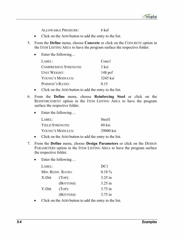
5-4 Examples
ALLOWABLE PRESSURE: 6 ksf • Click on the ADD button to add the entry to the list.
5. From the Define menu, choose Concrete or click on the CONCRETE option in the ITEM LISTING AREA to have the program surface the respective folder.
• Enter the following…
LABEL: Conc1 COMPRESSIVE STRENGTH: 3 ksi UNIT WEIGHT: 148 pcf YOUNG’S MODULUS: 3245 ksi POISSON’S RATIO: 0.15
• Click on the ADD button to add the entry to the list.
6. From the Define menu, choose Reinforcing Steel or click on the REINFORCEMENT option in the ITEM LISTING AREA to have the program surface the respective folder.
• Enter the following…
LABEL: Steel1 YIELD STRENGTH: 60 ksi YOUNG’S MODULUS: 29000 ksi
• Click on the ADD button to add the entry to the list.
7. From the Define menu, choose Design Parameters or click on the DESIGN PARAMETERS option in the ITEM LISTING AREA to have the program surface the respective folder.
• Enter the following…
LABEL: DC1 MIN. REINF. RATIO: 0.18 % X-DIR (TOP): 3.25 in
(BOTTOM): 3.25 in Y-DIR (TOP): 3.75 in
(BOTTOM): 3.75 in • Click on the ADD button to add the entry to the list.
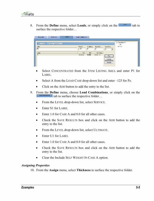
Examples 5-5
8. From the Define menu, select Loads, or simply click on the tab to surface the respective folder…
• Select CONCENTRATED from the ITEM LISTING AREA and enter P1 for
LABEL.
• Select A from the LOAD CASE drop-down list and enter –125 for Pz.
• Click on the ADD button to add the entry to the list.
9. From the Define menu, choose Load Combinations, or simply click on the tab to surface the respective folder…
• From the LEVEL drop-down list, select SERVICE.
• Enter S1 for LABEL
• Enter 1.0 for CASE A and 0.0 for all other cases.
• Check the SAVE RESULTS box and click on the ADD button to add the entry to the list.
• From the LEVEL drop-down list, select ULTIMATE.
• Enter U1 for LABEL
• Enter 1.0 for CASE A and 0.0 for all other cases.
• Check the SAVE RESULTS box and click on the ADD button to add the entry to the list.
• Clear the Include SELF WEIGHT IN CASE A option.
Assigning Properties 10. From the Assign menu, select Thickness to surface the respective folder.

5-6 Examples
• From the ITEM LISTING AREA, select THICK1.
• In the GRAPHICS/INPUT AREA, marquee-select the region (-1, 11)-(11, -1) to apply the selected thickness to the entire footing. The selected elements are redrawn in red.
Note: To see the assigned element and node numbers, from the Define menu, select Grid, and once the GRID folder surfaces, double click on PREFERENCES.
11. From the Assign menu, select Soil or click on the SOIL option in the ITEM LISTING AREA.
• Expand the SOIL listing in the ITEM LISTING AREA and select SOIL1.
• In the GRAPHICS/INPUT AREA, marquee-select the region (-1, 11)-(11, -1) to apply the selected soil to the entire footing. The selected elements are redrawn in red.
12. Repeat the step above using the Assign / Concrete, Assign / Reinforcing Steel and Assign / Design Parameters commands to apply CONCRETE1, STEEL1 and DC1 properties to the entire footing.
13. From the Assign menu, select Nodal Loads or simply click on the tab to surface the respective folder.
• In the ITEM LISTING AREA, expand Case A and then expand Concentrated to select P1.
• In the GRAPHICS AREA, click on each of the four nodes (4, 4), (6, 4), (4, 6) and (6,6). Small red squares are shown indicating loaded nodes…
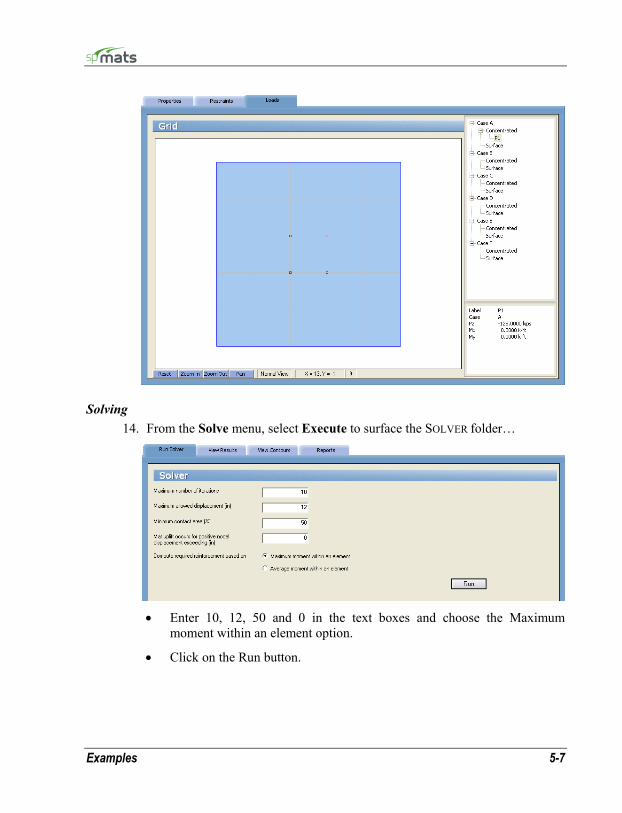
Examples 5-7
Solving 14. From the Solve menu, select Execute to surface the SOLVER folder…
• Enter 10, 12, 50 and 0 in the text boxes and choose the Maximum
moment within an element option.
• Click on the Run button.
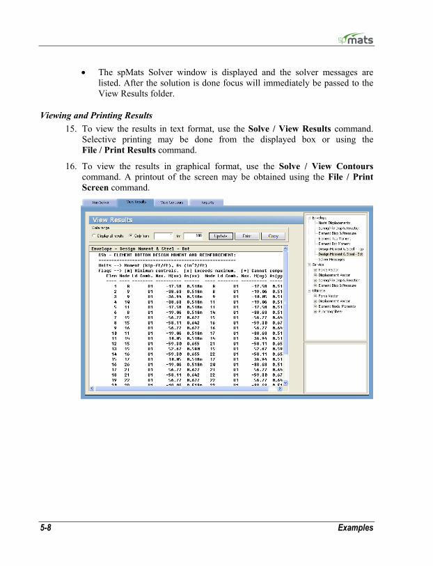
5-8 Examples
• The spMats Solver window is displayed and the solver messages are listed. After the solution is done focus will immediately be passed to the View Results folder.
Viewing and Printing Results 15. To view the results in text format, use the Solve / View Results command.
Selective printing may be done from the displayed box or using the File / Print Results command.
16. To view the results in graphical format, use the Solve / View Contours command. A printout of the screen may be obtained using the File / Print Screen command.

Examples 5-9
Element and Node Numbering for Example 1
Displacement contours for Example 1
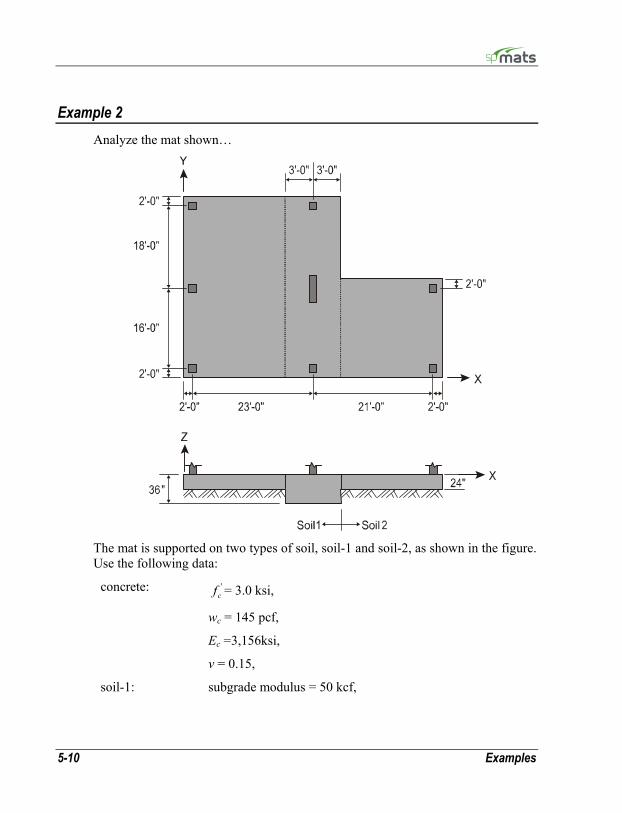
5-10 Examples
Example 2 Analyze the mat shown…
The mat is supported on two types of soil, soil-1 and soil-2, as shown in the figure. Use the following data:
concrete: 'cf = 3.0 ksi,
wc = 145 pcf,
Ec =3,156ksi,
v = 0.15,
soil-1: subgrade modulus = 50 kcf,
Examples 5-11
allowable pressure = 6 ksf,
soil-2: subgrade modulus = 75 kcf,
allowable pressure = 8 ksf,
steel: fy = 60 ksi,
Es = 29,000 ksi.
The superstructure was analyzed for wind loads. The resulting reactions for the columns and wall, as well as the dead and live loads, are as follows:
Dead Live Wind
Column Pz (kip) -50 -35 -10
Mx (ft-kip) 0 0 5
My (ft-kip) 0 0 0
Wall Pz (kip) -376 -208 -80
Mx (ft-kip) 0 0 60
My (ft-kip) 0 0 0
The mat will be analyzed for three service combinations and three ultimate combinations. Deflections and pressures are to be checked for the service combinations and the mat will be designed (compute required reinforcement) for the ultimate combinations.
Service Combinations: S1 = D+L S2 = D + L + W S3 = D + W
Ultimate Combinations: U1 = 1.4 D U2 = 1.2 D + 1.6 L U3 = 1.2 D + 1.0 L U4 = 1.2 D + 0.8 W U5 = 1.2 D + 1.0 L + 1.6 W U6 = 0.9 D + 1.6 W U7 = 1.2 D - 0.8 W U8 = 1.2 D + 1.0 L - 1.6 W U9 = 0.9 D - 1.6 W

5-12 Examples
The lower left-hand corner of the mat is chosen as the origin of the grid system. The grid layout is shown at the end of this example.
Since the wall is spanning over five nodes (nodes 205, 229, 253, 277 and 291), the wall loads will be divided into equivalent nodal loads depending on the tributary length of each node. Furthermore, the Rx degrees of freedom of these five nodes are slaved to simulate the stiffening effect of the wall.
Wall Loading Conditions

Examples 5-13
Inputting Problem Databases 1. From the Define menu, select General Info to surface the DESCRIPTION
folder…
• Input the project information and select ENGLISH units along with the ACI
318-05 code. Notice how the current date and time is displayed by default.
2. From the Define menu, select Grid, or simply click on the tab to surface the respective folder.
The X-Grid will be created in three parts as per the illustration below…
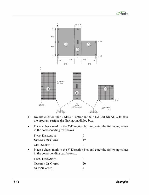
5-14 Examples
• Double-click on the GENERATE option in the ITEM LISTING AREA to have
the program surface the GENERATE dialog box.
• Place a check mark in the X-Direction box and enter the following values in the corresponding text boxes…
FROM DISTANCE: 0 NUMBER OF GRIDS: 12 GRID SPACING: 2
• Place a check mark in the Y-Direction box and enter the following values in the corresponding text boxes…
FROM DISTANCE: 0 NUMBER OF GRIDS: 20 GRID SPACING: 2
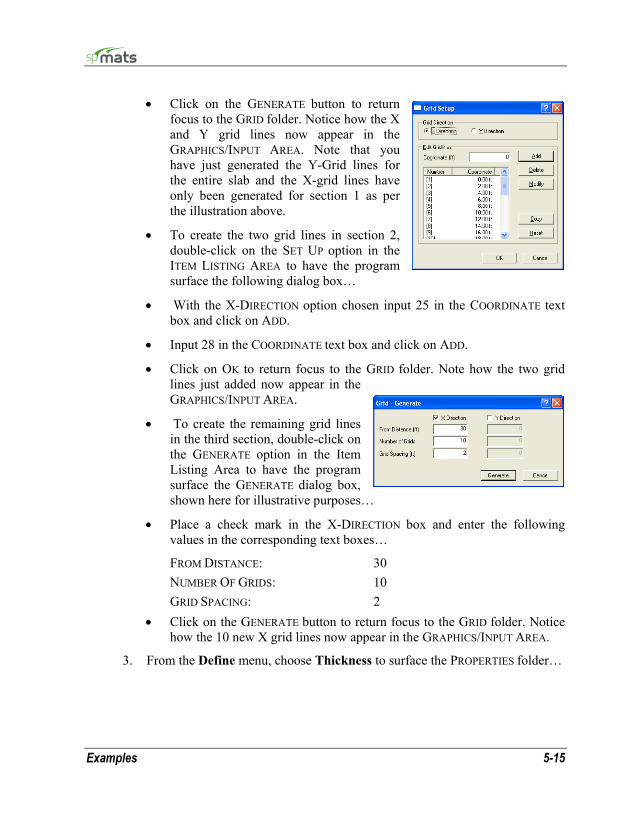
Examples 5-15
• Click on the GENERATE button to return focus to the GRID folder. Notice how the X and Y grid lines now appear in the GRAPHICS/INPUT AREA. Note that you have just generated the Y-Grid lines for the entire slab and the X-grid lines have only been generated for section 1 as per the illustration above.
• To create the two grid lines in section 2, double-click on the SET UP option in the ITEM LISTING AREA to have the program surface the following dialog box…
• With the X-DIRECTION option chosen input 25 in the COORDINATE text box and click on ADD.
• Input 28 in the COORDINATE text box and click on ADD.
• Click on OK to return focus to the GRID folder. Note how the two grid lines just added now appear in the GRAPHICS/INPUT AREA.
• To create the remaining grid lines in the third section, double-click on the GENERATE option in the Item Listing Area to have the program surface the GENERATE dialog box, shown here for illustrative purposes…
• Place a check mark in the X-DIRECTION box and enter the following values in the corresponding text boxes…
FROM DISTANCE: 30 NUMBER OF GRIDS: 10 GRID SPACING: 2
• Click on the GENERATE button to return focus to the GRID folder. Notice how the 10 new X grid lines now appear in the GRAPHICS/INPUT AREA.
3. From the Define menu, choose Thickness to surface the PROPERTIES folder…

5-16 Examples
• Input Thick1 for LABEL and 24.0 for THICKNESS.
• Click on the ADD button to add the entry to the list.
• Input Thick21 for LABEL and 36.0 for THICKNESS.
• Click on the ADD button to add the entry to the list.
4. From the Define menu, choose Soil, or click on the SOIL option in the ITEM LISTING AREA to have the program surface the respective folder.
• Enter the following…
LABEL: Soil1 SUBGRADE MODULUS: 50 kcf ALLOWABLE PRESSURE: 6 ksf
• Click on the ADD button to add the entry to the list.
• Enter the following…
LABEL: Soil2 SUBGRADE MODULUS: 75 kcf ALLOWABLE PRESSURE: 8 ksf

Examples 5-17
• Click on the ADD button to add the entry to the list.
5. From the Define menu, choose Concrete or click on the CONCRETE option in the ITEM LISTING AREA to have the program surface the respective folder.
• Enter the following… LABEL: Conc1
COMPRESSIVE STRENGTH: 3 ksi UNIT WEIGHT: 145 pcf YOUNG’S MODULUS: 3156 ksi POISSON’S RATIO: 0.15
• Click on the ADD button to add the entry to the list.
6. From the Define menu, choose Reinforcing Steel or click on the REINFORCEMENT option in the ITEM LISTING AREA to have the program surface the respective folder.
• Enter the following…
LABEL: Steel1 YIELD STRENGTH: 60 ksi YOUNG’S MODULUS: 29000 ksi
• Click on the ADD button to add the entry to the list.
7. From the Define menu, choose Design Parameters or click on the DESIGN PARAMETERS option in the ITEM LISTING AREA to have the -program surface the respective folder.
• Enter the following…
LABEL: DC1 MIN. REINF. RATIO: 0.18 % X-DIR (TOP): 3.25 in (BOTTOM): 3.25 in Y-DIR (TOP): 3.50 in
(BOTTOM): 3.50 in • Click on the ADD button to add the entry to the list.
8. From the Define menu, choose Column Dimensions or click on the COLUMN DIMENSIONS option in the ITEM LISTING AREA to have the program surface the respective folder.
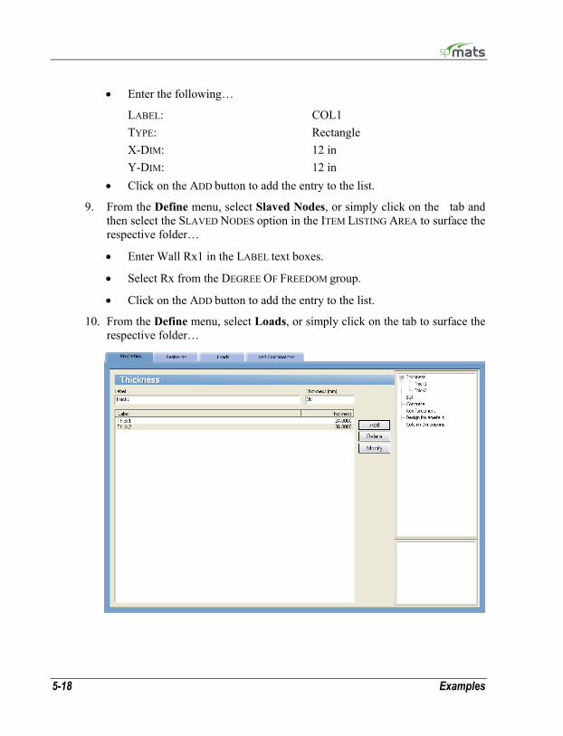
5-18 Examples
• Enter the following…
LABEL: COL1 TYPE: Rectangle X-DIM: 12 in Y-DIM: 12 in
• Click on the ADD button to add the entry to the list.
9. From the Define menu, select Slaved Nodes, or simply click on the tab and then select the SLAVED NODES option in the ITEM LISTING AREA to surface the respective folder…
• Enter Wall Rx1 in the LABEL text boxes.
• Select Rx from the DEGREE OF FREEDOM group.
• Click on the ADD button to add the entry to the list.
10. From the Define menu, select Loads, or simply click on the tab to surface the respective folder…
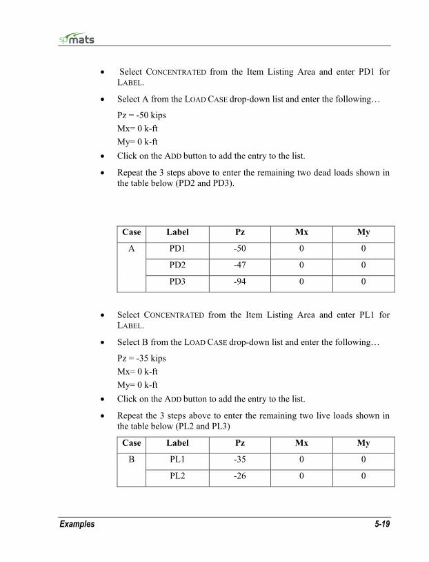
Examples 5-19
• Select CONCENTRATED from the Item Listing Area and enter PD1 for LABEL.
• Select A from the LOAD CASE drop-down list and enter the following…
Pz = -50 kips Mx= 0 k-ft My= 0 k-ft
• Click on the ADD button to add the entry to the list.
• Repeat the 3 steps above to enter the remaining two dead loads shown in the table below (PD2 and PD3).
Case Label Pz Mx My
PD1 -50 0 0
PD2 -47 0 0
A
PD3 -94 0 0
• Select CONCENTRATED from the Item Listing Area and enter PL1 for
LABEL.
• Select B from the LOAD CASE drop-down list and enter the following…
Pz = -35 kips Mx= 0 k-ft My= 0 k-ft
• Click on the ADD button to add the entry to the list.
• Repeat the 3 steps above to enter the remaining two live loads shown in the table below (PL2 and PL3)
Case Label Pz Mx My
PL1 -35 0 0 B
PL2 -26 0 0
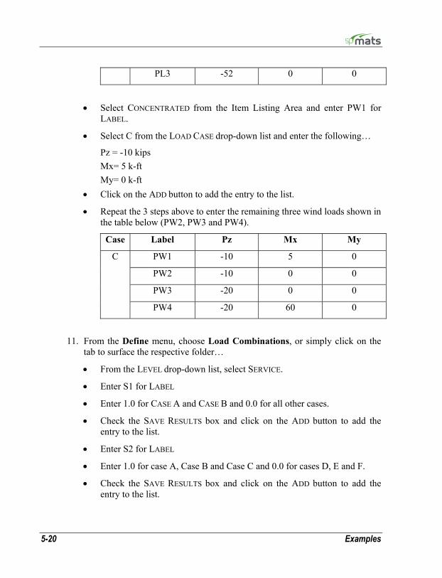
5-20 Examples
PL3 -52 0 0
• Select CONCENTRATED from the Item Listing Area and enter PW1 for
LABEL.
• Select C from the LOAD CASE drop-down list and enter the following…
Pz = -10 kips Mx= 5 k-ft My= 0 k-ft
• Click on the ADD button to add the entry to the list.
• Repeat the 3 steps above to enter the remaining three wind loads shown in the table below (PW2, PW3 and PW4).
Case Label Pz Mx My
PW1 -10 5 0
PW2 -10 0 0
PW3 -20 0 0
C
PW4 -20 60 0
11. From the Define menu, choose Load Combinations, or simply click on the
tab to surface the respective folder…
• From the LEVEL drop-down list, select SERVICE.
• Enter S1 for LABEL
• Enter 1.0 for CASE A and CASE B and 0.0 for all other cases.
• Check the SAVE RESULTS box and click on the ADD button to add the entry to the list.
• Enter S2 for LABEL
• Enter 1.0 for case A, Case B and Case C and 0.0 for cases D, E and F.
• Check the SAVE RESULTS box and click on the ADD button to add the entry to the list.
Examples 5-21
• Enter S3 for LABEL and 1.0 for Case A and Case C. Enter 0.0 for all other cases.
• Check the SAVE RESULTS box and click on the ADD button to add the entry to the list.
• From the LEVEL drop-down list, select ULTIMATE and enter U1 for LABEL.
• Enter 1.4 for CASE A, and 0.0 for all other cases.
• Check the SAVE RESULTS box and click on the ADD button to add the entry to the list.
• Enter U2 for LABEL and 1.2 for CASE A, 1.6 for CASE B, and 0.0 for all other cases.
• Check the SAVE RESULTS box and click on the ADD button to add the entry to the list.
• Enter U3 for LABEL
• Enter 1.2 for CASE A, 1.0 for CASE B, and 0.0 for all other cases.
• Check the SAVE RESULTS box and click on the ADD button to add the entry to the list.
• Enter U4 for LABEL
• Enter 1.2 for CASE A, 0.8 for CASE C, and 0.0 for all other cases.
• Check the SAVE RESULTS box and click on the ADD button to add the entry to the list.
• Enter U5 for LABEL
• Enter 1.2 for CASE A, 1.0 for CASE B, 1.6 for CASE C and 0.0 for all other cases.
• Check the SAVE RESULTS box and click on the ADD button to add the entry to the list.
• Enter U6 for LABEL
• Enter 0.9 for CASE A, 1.6 for CASE C, and 0.0 for all other cases.
• Check the SAVE RESULTS box and click on the ADD button to add the entry to the list.

5-22 Examples
• Enter U7 for LABEL
• Enter 1.2 for CASE A, -0.8 for CASE C, and 0.0 for all other cases.
• Check the SAVE RESULTS box and click on the ADD button to add the entry to the list.
• Enter U8 for LABEL
• Enter 1.2 for CASE A, 1.0 for CASE B, -1.6 for CASE C, and 0.0 for all other cases.
• Check the SAVE RESULTS box and click on the ADD button to add the entry to the list.
• Enter U9 for LABEL
• Enter 0.9 for CASE A, -1.6 for CASE C, and 0.0 for all other cases.
• Check the SAVE RESULTS box and click on the ADD button to add the entry to the list.
• Clear the Include SELF WEIGHT IN CASE A option.
Assigning Properties 12. From the Assign menu, select Thickness to surface the respective folder.
• From the ITEM LISTING AREA, select THICK1.
• In the GRAPHICS/INPUT AREA, marquee-select the region (-1,39) – (23, -1) to apply the selected thickness to that part of the footing.
• Marquee-select the region (27,21) – (49, -1) to apply the selected thickness to that part of the footing. Notice how the selected regions are redrawn in red…
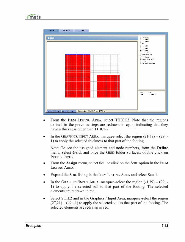
Examples 5-23
• From the ITEM LISTING AREA, select THICK2. Note that the regions
defined in the previous steps are redrawn in cyan, indicating that they have a thickness other than THICK2.
• In the GRAPHICS/INPUT AREA, marquee-select the region (21,39) – (29, -1) to apply the selected thickness to that part of the footing.
Note: To see the assigned element and node numbers, from the Define menu, select Grid, and once the GRID folder surfaces, double click on PREFERENCES.
• From the Assign menu, select Soil or click on the SOIL option in the ITEM LISTING AREA.
• Expand the SOIL listing in the ITEM LISTING AREA and select SOIL1.
• In the GRAPHICS/INPUT AREA, marquee-select the region (-1,39) – (29, -1) to apply the selected soil to that part of the footing. The selected elements are redrawn in red.
• Select SOIL2 and in the Graphics / Input Area, marquee-select the region (27,21) – (49, -1) to apply the selected soil to that part of the footing. The selected elements are redrawn in red.

5-24 Examples
13. From the Assign menu, select Concrete or click on the CONCRETE option in the ITEM LISTING AREA.
• Expand the CONCRETE listing in the ITEM LISTING AREA and select CONC1.
• In the GRAPHICS/INPUT AREA, marquee-select the region (-1, 39) – (49, -1) to apply the selected concrete to the entire footing. The selected elements are redrawn in red.
14. Repeat the step above using the Assign / Reinforcing Steel and Assign / Design Parameters commands to apply STEEL1 and DC1 properties to the entire footing.
15. From the Assign menu, select Column Dimensions or click on the COLUMN DIMENSIONS option in the ITEM LISTING AREA.
• Expand the COLUMN DIMENSIONS listing in the ITEM LISTING AREA and select COL1.
• In the GRAPHICS AREA, click on each of the following nodes (2,2), (25,2), (46,2), (2,18), (46,18), (2,36) and (25,36). Column sections are shown indicating columns are assigned.
16. From the Assign menu, select Slaved Loads or simply click on the tab to surface the respective folder.
• In the ITEM LISTING AREA, expand the SLAVED NODES item to display WallRx1 – select it.
• In the GRAPHICS AREA, marquee-select the region (24,25) – (26,15). The five nodes within the selected region are redrawn in red. These nodes are assigned to the slaved nodes group WallRx1.
17. From the Assign menu, select Nodal Loads or simply click on the tab to surface the respective folder.
• In the ITEM LISTING AREA, expand Case A and then expand CONCENTRATED to select PD1.
• In the GRAPHICS AREA, click on each of the following nodes (2,2), (25,2), (46,2), (2,18), (46,18), (2,36) and (25,36). Small red squares are shown indicating loaded nodes. Note that it is important to assign column nodal load to the same nodes where columns are assigned in step 15 in order for punching shear to be calculated properly.
Examples 5-25
• Select PD2 from the list box. In the GRAPHICS AREA, click on the nodes (25,14) and (25,22).
• Select PD3 from the list box. In the GRAPHICS AREA, click on the nodes (25,16), (25,18) and (25,20).
• In the ITEM LISTING AREA, expand Case B and then expand CONCENTRATED to select PL1.
• In the GRAPHICS AREA, click on each of the following nodes (2,2), (25,2), (46,2), (2,18), (46,18), (2,36) and (25,36).
• Select PL2 from the list box. In the GRAPHICS AREA, click on the nodes (25,14) and (25,22).
• Select PL3 from the list box. In the GRAPHICS AREA, click on the nodes (25,16), (25,18) and (25,20).
• In the ITEM LISTING AREA, expand Case C and then expand CONCENTRATED to select PW1.
• In the GRAPHICS AREA, click on each of the following nodes (2,2), (25,2), (46,2), (2,18), (46,18), (2,36) and (25,36).
• Select PW2 from the list box. In the GRAPHICS AREA, click on the nodes (25,16) and (25,24).
• Select PW3 from the list box. In the GRAPHICS AREA, click on the nodes (25,18) and (25,22).
• Select PW4 from the list box. In the GRAPHICS AREA, click on the node (25,20).
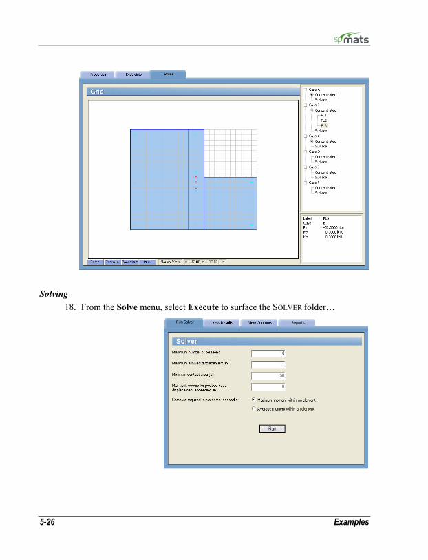
5-26 Examples
Solving 18. From the Solve menu, select Execute to surface the SOLVER folder…

Examples 5-27
• Enter 10, 12, 50 and 0 in the text boxes and choose the MAXIMUM MOMENT WITHIN AN ELEMENT option.
• Click on the RUN button.
• The spMats Solver window is displayed and the solver messages are listed. After the solution is done focus will automatically be passed to the VIEW RESULTS folder.
Viewing and Printing Results 19. To view the results in text format, use the Solve / View Results command.
Selective printing may be done from the displayed box or using the File / Print Results command.
20. To view the results in graphical format, use the Solve / View Contours command. A printout of the screen may be obtained using the File / Print Screen command.
Sample Results for Example 2

5-28 Examples
Service Envelope Displacement Contours for Example 2
Element Numbering for Example 2
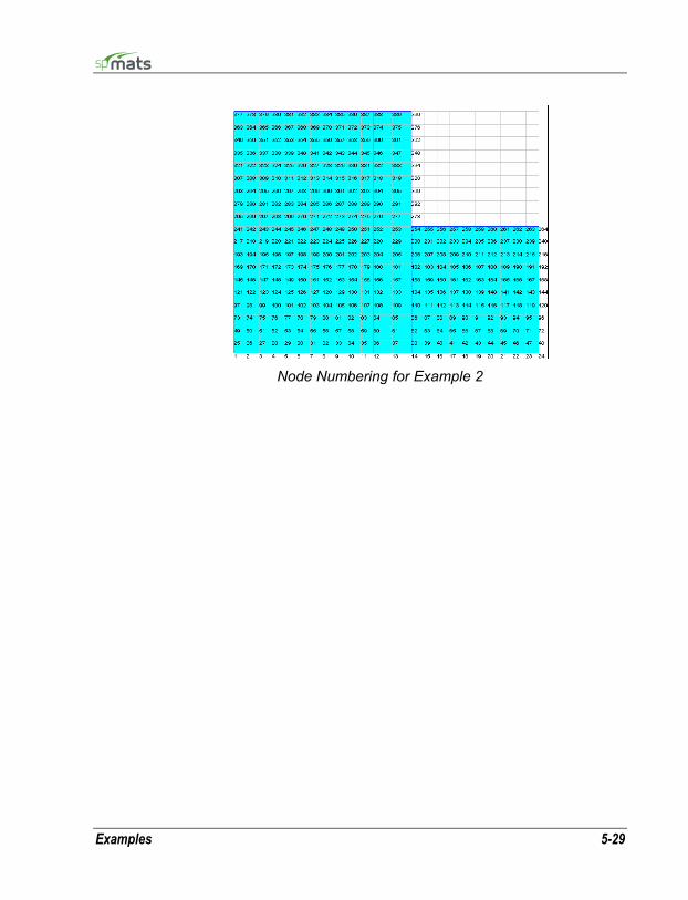
Examples 5-29
Node Numbering for Example 2

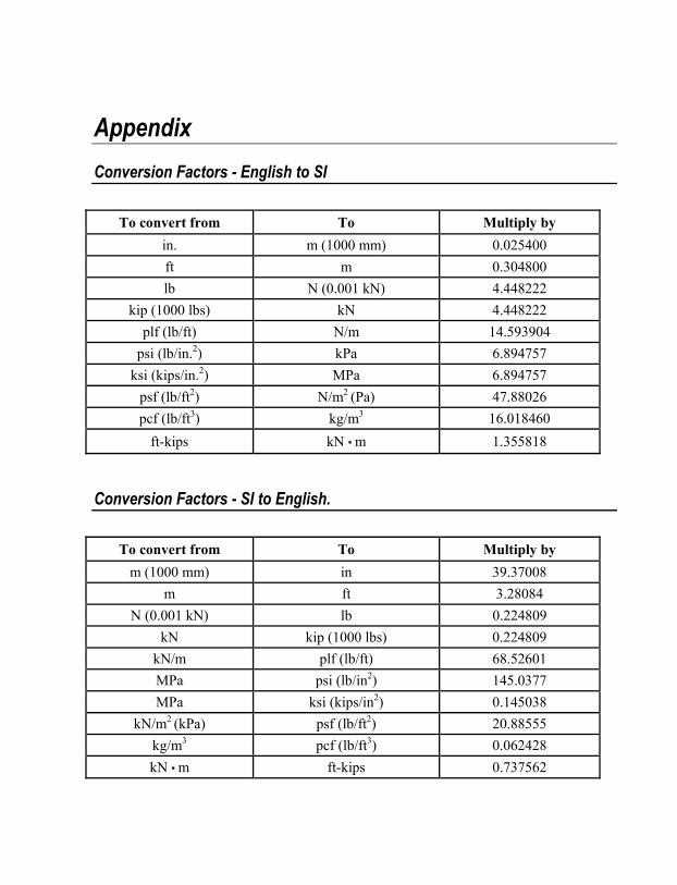
Appendix Conversion Factors - English to SI
To convert from To Multiply by
in. m (1000 mm) 0.025400 ft m 0.304800 lb N (0.001 kN) 4.448222
kip (1000 lbs) kN 4.448222 plf (lb/ft) N/m 14.593904
psi (lb/in.2) kPa 6.894757 ksi (kips/in.2) MPa 6.894757
psf (lb/ft2) N/m2 (Pa) 47.88026 pcf (lb/ft3) kg/m3 16.018460
ft-kips kN • m 1.355818
Conversion Factors - SI to English.
To convert from To Multiply by m (1000 mm) in 39.37008
m ft 3.28084 N (0.001 kN) lb 0.224809
kN kip (1000 lbs) 0.224809 kN/m plf (lb/ft) 68.52601 MPa psi (lb/in2) 145.0377 MPa ksi (kips/in2) 0.145038
kN/m2 (kPa) psf (lb/ft2) 20.88555 kg/m3 pcf (lb/ft3) 0.062428 kN • m ft-kips 0.737562

A-2 Appendix
Contact Information
Mail: StructurePoint Customer Service 5420 Old Orchard Road Skokie, IL 60077 USA Phone: (847) 966-4357 Fax: (847) 966-1542 Web: http://www.StructurePoint.org Sales [email protected] Support [email protected] Licensing [email protected]