splitting methods for fourth-order image...
TRANSCRIPT

Splitting methodsfor fourth-order image inpainting
Luca CalatroniSupervisor: Dr. Carola Schonlieb
November 6, 2012
1 Image inpainting
One of the most important applications of image processing is the process offilling the missing parts of damaged images using the information obtainedfrom the surrounding areas. We can think of this process as, essentially, atype of interpolation called inpainting. Such a technique can be used forrestoring images within parts damaged due to, for example, wear and tear(like the restoration of ancient frescoes or the scratch removal in old pho-tographs) or for needs of reducing artifacts in MRI-imaging reconstructions.
From a mathematical point of view, image inpainting can be described asfollows: given an image f on an image domain Ω, the task is to reconstructthe original image u in the damaged domain D ⊂ Ω, called the inpaintingdomain (see Figure 1).
Figure 1: The inpainting problem: the image is missing on D which can havemany connected components with arbitrarily shapes and sizes.
Various approaches to solve this task exist in the literature. A basic divi-sion of inpainting methodologies yields two groups, global methods (interpo-lation is performed with all the available image contents) and local methods
1

(interpolation is based only on the surrounding parts of the image). In whatfollow, we will only consider methods from the latter class phrased as varia-tional problems or partial differential equations.
More precisely, let Ω ⊂ R2 be an open and bounded domain with Lipschitzboundary and let B1, B2 two Banach spaces with, typically, B2 ⊆ B1. Letf ∈ B1 denote the given image and D ⊂ Ω the inpainting domain. A generalvariational approach in image inpainting can be generally formulated as aminimization problem for a functional E : B2 → R, that is:
minu∈B2
E(u) := R(u) + ‖λ(f − u)‖2
B1
(1)
where R : B2 → R denotes the regularizing term and
λ(x) :=
λ0 if x ∈ Ω \D0 if x ∈ D
is the characteristic function of the set Ω \D multiplied by a typically largeconstant λ0. The norm ‖λ(f − u)‖2
B1is the so called fidelity term of the in-
painting approach. The inclusion B2 ⊆ B1 in general represents the smooth-ing effect of R on the minimizer u. We note that such an approach posesthe inpainting problem in the whole domain Ω, not in the inpainting domainD. This allows us to deal even with inpainting problems in which D is notconnected and has arbitrary regularity features.
Depending on the choice of the regularizing term R and the spaces B1, B2,various inpainting approaches have been developed. Under some regularityassumptions on the minimizer u in (1), we can consider the correspondingEuler-Lagrange equation, just taking the Frechet derivative of the functionalE. The highest order of the derivatives of such an equation determines theso called order of the inpainting method used. In the case B1 = B2 = L2(Ω)with the choice R(u) = ‖∇u‖2, for instance, the underlying second orderPDE related to the minimization process is the following:
ut = −∆u+ λ(f − u) (2)
where the dependence on time arises by embedding the process into a steepest-descent. The equation (2) is then an example of second order method forinpainting, typically called linear inpainting.
Second order variational inpainting methods (like, for instance, (2) andthe TV model) have been largely used, but they present drawbacks in con-necting edges over large distances (thus failing the so-called connectivity prin-ciple) and in the smooth propagation of level lines into the damaged domain.The reason is due to the penalization of the length within the minimizing
2

process with a second order regularizer (see [13, Section 1.2] for further de-tails).
In order to solve such a problem, some higher order methods have beendeveloped, at first using third-order methods (see, e.g., Bertalmio et al. [2]),then using fourth-order methods (as the Eulers elastica models presented in[5], the Cahn-Hilliard [3] and TV-H−1 [4] ones) . For the well-posednessof these problems another boundary condition is required, but on the otherhand they are able to fulfill the connectivity principle.
From a numerical point of view, discretizing explicitly a fourth-order evo-lution equation may restrict the time-step ∆t up to order (∆x)4 where ∆xdenotes the step size of the spatial grid: this kind of methods requires ahuge amount of iterations and then these methods are computationally pro-hibitive. Efficient numerical schemes for inpainting methods of higher-orderis an active area of research. In this work we present some methods developedto solve this problem based on a general idea presented in the next section.
2 The splitting idea
The general idea behind any so called splitting method is breaking down acomplicated problem into smaller (and, typically, easier to approach) parts,such that these smaller problems can be solved efficiently. Different splittingmethods have been presented both to solve ODEs and PDEs. The main ideais the splitting of the operator defining the problem into different components.A particular case of operator splitting is the dimensional splitting where thedecompositions is performed such that all the computations become actuallyone-dimensional. Typically, the original problem is decomposed into more-manageable substeps (called fractional steps) which yield approximations ofthe solution of the full problem, but which, generally, are not consistent. Inthe following subsection we present some general examples of operator split-ting methods. Namely, we describe Strang splitting and convexity splittingmethods and, as example of dimensional splitting, the alternating directionimplicit (ADI) methods. In the next section we will apply them to the prob-lem of inpainting.
2.1 A second-order symmetrical splitting method: theStrang splitting
Let us consider a linear, homogeneous ODE system with an initial condition:
u′(t) = Au(t), t > 0, u(0) = u0 (3)
3

and assume that the operator A can be splitted as A = A1 +A2. Consideringa uniform time-discretized grid with nodes ti, i ≥ 1 and setting ∆t := tn+1−tnfor every n, we know that the solution of (3) is given by:
u(tn+1) = e∆tAu(tn). (4)
Indicating with un the approximation of the exact solution at the point tn,that is un ≈ u(tn), we can introduce for every time step n− n + 1 a middlestep n+ 1/2 and solving auxiliary problems starting from un to obtain un+1.Solving at first:
d
dtu∗(t) = A1u
∗(t) for tn < t ≤ tn+1/2 with u∗(tn) = un
d
dtu∗∗(t) = A2u
∗∗(t) for tn < t ≤ tn+1/2 with u∗∗(tn) = u∗(tn+1/2)
(5)
one after another starting from un, we can take un+1/2 = u∗∗(tn+1/2), thuscompleting the half step. We can now redo the same, interchanging the orderof application of A1 and A2, starting now from un+1/2 and solving
d
dtu?(t) = A2u
?(t) for tn+1/2 < t ≤ tn+1 with u?(tn+1/2) = un+1/2
d
dtu??(t) = A1u
??(t) for tn+1/2 < t ≤ tn+1 with u??(tn+1/2) = u?(tn+1)
(6)one after another, taking un+1 = u??(un+1) to complete the splitting integra-tion step. This gives:
un+1 = e∆t2A1e
∆t2A2un+1/2 =
(e
∆t2A1e
∆t2A2
)(e
∆t2A2e
∆t2A1
)un
= e∆t2A1e∆tA2e
∆t2A1un (7)
which leads symmetry and accuracy to the problem. Of course, replacing (4)by (7) introduces an error, the splitting error. Inserting the exact solution uto the original problem into (7), we have:
u(tn+1) = e∆t2A1e∆tA2e
∆t2A1u(tn) + ∆tρn
where ρn is the local truncation error. By series expansion it is possible toshow that ρn is of order two, thus revealing a formal consistency of suchan order. Generalization of such method exists both in the case the stepsize ∆t is not constant and when the operator splitting has more than twocomponents. For further details see [11].
4

2.2 Convexity splitting
The idea of convexity splitting was originally introduced to solve energy min-imizing equations (see [7]): let V ∈ C2(Rn,R) a functional. Let Ω be thespatial domain of the data. We consider the following problem:
find u ∈ RN such that
ut = −∇V (u) in Ω
u(·, 0) = u0 in Ω.(8)
The main idea of convexity splitting is to split the functional V into a convexand a concave part, that is decomposing V as:
V (u) = Vc(u)− Ve(u)
where both Vc and Ve are strictly convex for all u ∈ Rn. We can write downthen a semi-implicit discretization of (8) given by:
Uk+1 − Uk = −∆t(∇Vc(Uk+1)−∇Ve(Uk)).
where by Uk we indicate the numerical approximation of u(k∆t). As weare going to see in the following, the convexity splitting idea can be appliedalso to more general evolution equations, in particular to those which donot follow a variational principle 1. Such methods have a long tradition inseveral parts of numerical analysis. They have been applied in finite elementand finite difference approximations (see [7], [14] and [13])). Using a semi-implicit discretization scheme, the application of such a method consists intreating implicitly in time the convex part and explicitly the concave one,thus having a balance between the nice properties of convex functions andthe computational effort to solve implicit methods.
2.3 The ADI method
Consider the initial value problem for a system of ODEs:u′(t) = F (t, u(t)) in [0, T ]
u(0) = u0
and suppose that it is possible to decompose the function F into a numberof component functions such that each of these components acts just on onesingle direction of the space, that is:
F (t, v) = F0(t, v) + F1(t, v) + · · ·+ Fs(t, v) for some s ≥ 1 (9)
1We recall that saying that the solutions of Euler-Lagrange equations follow a varia-tional principle means that they cause the vanish of the Frechet derivative.
5

where the component Fj, 1 ≤ j ≤ s is acting in the j-th direction of Rs. Wedefine now a method which uses decomposition (9) by treating in each stageof the calculation at most one of the components Fi implicitly. We assumeinstead that the F0 component can be treated explicitly (or, equivalently, itis not stiff) and contains contributes coming from mixed directions, whereasthe Fj, j ≥ 1 are stiff and so they need an implicit treatment. We considerthe following scheme, the so-called ADI Douglas method, depending on aparameter θ > 0:
v0 = un + ∆tF (tn, un),
vj = vj−1 + θ∆t(Fj(tn+1, vj)− Fj(tn, un)) for j = 1, 2, . . . , s,
un+1 = vs
(10)
where the vj are the internal vectors for the step from tn to tn+1 and we haveused the same notation as in Section 2.1. Heuristically, the calculation ofvectors vj, j = 1, . . . , s serves to stabilize the forward Euler method used tocalculate v0. It can be verified that the order of the scheme (10) is equal to2 whenever F0 = 0 and θ = 1/2 and it is of order 1 otherwise (see [11]).
Some extension of the Douglas method has been suggested in order toincrease the order of the method independently of F0 (see [9], [10]): thisis basically done introducing further additional stages which, however, donot badly influenced the property of unconditional stability of such methods,which holds in any case. These methods have been largely applied in thestudy of convection-diffusion equations such as in financial option pricing.In this work we will use a suitable generalization of (10), applying it to ourproblem of inpainting.
3 Inpainting models based on splitting ideas
We present now some meaningful applications of the presented splittingmethods to the problem of inpainting presented in Section 1. We pointout that the models (5)-(6) and (10) refer to the solution of ODEs systemwhile the methods we are going to deal with are based on a PDE approach.However, as it is well-known, discretizing the spatial derivatives of an evolu-tion PDE with finite differences we get exactly very large systems of ODEs.We can then apply the splitting technique in these cases.
3.1 TV-H−1 inpainting
We present now a recently proposed approach to inpainting for grayvaluesimages, called TV-H1 inpainting (see [13] for further details). It can be seen
6
as a generalization of the Cahn-Hilliard inpainting approach for grayvaluesimage. In TV-H1 method the inpainted image u of the given image f ∈ L2(Ω)evolves via:
ut = −∆ξ + λ(f − u)
ξ ∈ ∂TV (u)
where the total variation TV (u) is defined as:
TV (u) :=
|Du|(Ω) if ‖u‖∞ ≤ 1 a.e. in Ω
+∞ otherwise.
For the definition of the quantities involved see Appendices A-B. TheL∞-bound of the functional TV (u) is justified remembering that we are onlyconsidering images u which take values just in the interval [−1, 1] whichcorresponds to the grayvalues taken by u. In our approach we approximatethe element ξ by the square root regularization of ∇ · (∇u/|∇u|), i.e. weconsider for 0 < ε 1 the smoothed approximation given by:
ut = −∆∇ ·(∇u|∇u|ε
)+ λ(f − u) (11)
where, for notational simplicity we write |∇u|ε to indicate the regularizingterm
√|∇u|2 + ε.
3.1.1 Convexity splitting for TV-H−1 inpainting
We present an application of a convexity splitting method to solve (11).Equation (11) is not a gradient system (see (8)), nonetheless we can considertwo different gradient flows and apply the splitting idea separately. Theregularizing term can be modeled by a gradient flow in H−1 (i.e. taking theFrechet derivative with respect to the H−1 norm) of the energy:
E1(u) :=
∫Ω
|∇u(x)|εdx.
Now, we split E1 as E1,c − E1,e, with
E1,c(u) :=
∫Ω
C1
2|∇u(x)|2εdx and
E1,e(u) :=
∫Ω
(−|∇u(x)|ε +
C1
2|∇u(x)|2ε
)dx.
7

where the constant C1 has to be chosen such that E1,c and E1,e are strictlyconvex. As E1,c is strictly convex for every choice of C1, the convexity condi-tion for the second derivative for E1,e gives easily that C1 >
1√ε. The second
term of (11) can be derived instead from a gradient flow in L2 for the energy:
E2(u) :=
∫Ω
(λ(x)(f(x)− u(x)))2dx.
Now we split E2 as E2,c − E2,e with
E2,c(u) :=1
2
∫Ω
C2|u(x)|2dx and
E2,e(u) :=1
2
∫Ω
(−(λ(x)(f(x)− u(x)))2 + C2|u(x)|2
)dx
where now the constant C2 has to be chosen such that C2 > λ0. Denoting byUk the solution of the time-discrete equation at time k∆t, we have that theresulting semi-implicit discrete time-stepping scheme for an initial conditionU0 = u0 is:
Uk+1 − Uk∆t
= −δH−1(E1,c(Uk+1)− E1,e(Uk))− δL2(E2,c(Uk+1 − E2,e(Uk))
where δH−1 and δL2 represent the Frechet derivatives with respect to the normin H−1 and L2, respectively.
Here the quantities are assumed to be discretized in space as follows: thediscrete gradient ∇ is computed using forward differences, the divergence∇· using backward differences and then the Laplacian is defined by ∇ · ∇.Hence, the resulting scheme is given by:
Uk+1 − Uk∆t
+ C1∆2Uk+1 + C2Uk+1 (12)
= C1∆2Uk −∆
(∇ ·(∇Uk|∇Uk|ε
))+ C2Uk + λ(f − Uk).
Assuming zero Neumann boundary conditions on ∂Ω, that is ∇Uk+1 · ν =∇∆Uk+1 ·ν = 0 on ∂Ω, we can solve (12) using the discrete cosine transform.Now we state the main results concerning such scheme, summarizing themin the following theorem ([13, Theorem 4.1]):
Theorem 3.1 (Consistency, Stability, Convergence). Let u be the exact solu-tion of (11) and uk = u(k∆t) the exact solution evaluated at time k∆t, k ∈ N.Let Uk the kth iterate of (12) with constant C1 > 1/
√ε and C2 > λ0. Then,
for any T > 0 fixed and every k∆t ≤ T :
8

1. If ‖utt‖H−1 and ‖∇∆ut‖L2 are bounded, then the numerical scheme (12)is consistent with the continuous equation (11) with local truncationerror ‖∆tk‖H−1 = O(∆t).
2. For every ∆t > 0:
‖∇Uk‖2L2+∆tK1 ‖∇∆Uk‖2
L2 ≤ eK2T (‖∇U0‖2L2+∆tK1 ‖∇∆U0‖2
L2+∆tTC)
for suitable constants K1, K2 and a constant C = C(Ω, D, λ0, f). Inother words, the sequence Uk is bounded on a finite interval [0, T ] forall ∆t > 0. We say that the method is unconditionally stable2.
3. Let ek := uk − Uk. We have:
‖∇ek‖2L2 + ∆tM1 ‖∇∆ek‖2
L2 ≤T
M2
eM3T (∆t)2
for suitable constants M1,M2 and M3. In other words, the error ekconverges to zero as ∆t→ 0.
We will not present here the proof of this Theorem, as it constitutes themain part of Section 4 of [13].
3.1.2 Strang splitting for TV-H−1 inpainting
We present now an application of the Strang splitting method presented in2.1 to solve in a different way our inpainting problem.In order to solve the fourth-order equation (11), we consider the system oftwo second-order equations given by:
ut = ∆v + λ(f − u),
v = −∇ · ( ∇u|∇u| ε
).
Now we apply backward Euler temporal discretization an the Strang method,thus obtaining the following scheme:
Un+1/2 =Un + ∆t
2(∆Vn + λf)
1 + λ2
,
Vn+1/2 = −∇ ·(∇Un+1/2
|∇Un+1/2|ε
),
Un+1 =Un+1/2 + ∆t
2(∆Vn+1/2 + λf)
1 + λ2
.
(13)
2As we have seen, the TV-H−1 inpainting is not given by a single gradient flow, thenthe meaning of unconditional stability has to be refined in this way.
9
The spatial operators appearing in (13) are discretized in the same way asdone for the convexity splitting. Results as Theorem 3.1 about convergence,stability and consistency do not exist, so they represent an interesting areaof future research. We just point out that as the reader may note by himself,the scheme (13) is essentially an explicit method, then stability issues areexpected.
3.1.3 Numerical results
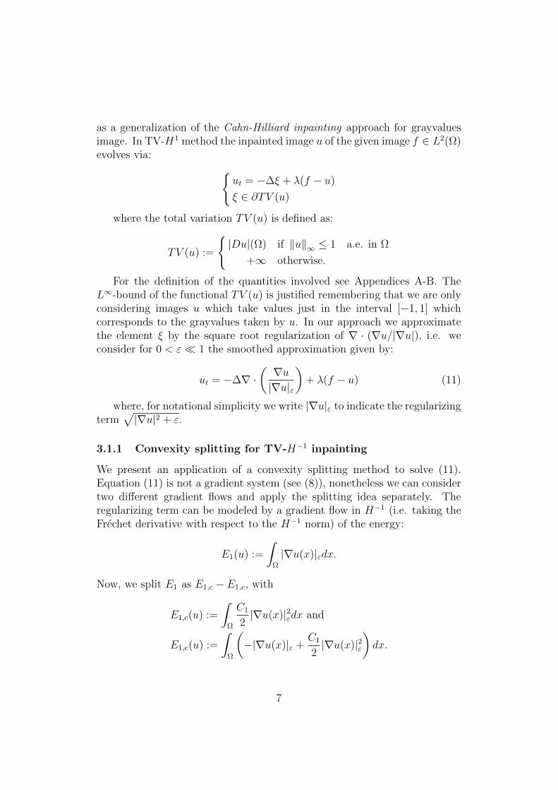
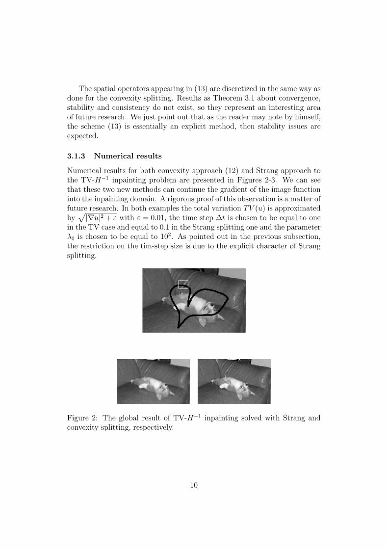
Numerical results for both convexity approach (12) and Strang approach tothe TV-H−1 inpainting problem are presented in Figures 2-3. We can seethat these two new methods can continue the gradient of the image functioninto the inpainting domain. A rigorous proof of this observation is a matter offuture research. In both examples the total variation TV (u) is approximatedby√|∇u|2 + ε with ε = 0.01, the time step ∆t is chosen to be equal to one
in the TV case and equal to 0.1 in the Strang splitting one and the parameterλ0 is chosen to be equal to 102. As pointed out in the previous subsection,the restriction on the tim-step size is due to the explicit character of Strangsplitting.
Figure 2: The global result of TV-H−1 inpainting solved with Strang andconvexity splitting, respectively.
10
Figure 3: The particular shows the continuation of the gradient for bothStrang and convexity splitting method.
4 Two new methods based on an ADI ap-
proach
In the following we will present two different ADI schemes to solve the in-painting problem. We will present both of them in the total variation frame-work, using once again the total variation square root regularization, i.e. wewill consider the PDE (11) as governing the problem. Numerical solution ofsuch an equation poses several problems:
• As pointed out in Section 1, the stiffness of fourth-order parabolic equa-tions like (11) lays down some constraints on the time-step size for ex-plicit methods typically of the type ∆t = O(∆x4) which make suchmethods prohibitive. Hence, implicit methods are necessary;
• The presence of |∇u|ε in (11) makes the equation strongly nonlinear,hence convergence and accuracy are important considerations;
• The spatial operator necessarily includes mixed derivative terms forwhich splitting schemes appear to be more complicated.
Sensible methods for finding the numerical solution of such a problemwere found by using a simpler equation, not directly related to problemsarising in image processing, but with the common feature of being of higherorder.
4.1 ADI-splitting schemes for the biharmonic equation
We exploit an auxiliary fourth order parabolic equation, called the bihar-monic equation. The behaviour of the solution of such an equation is verywell-known and it is then easy comparing the numerical results with whatwe expect.
11

4.1.1 The scheme applied to the whole equation
We are dealing with the following partial differential equation, defined onΩ× R+:
ut = −∆2u = −uxxxx − uyyyy − 2uxxyy = F (u). (14)
We would like to semi-discretize the equation (14) and perform an ADI-splitting scheme similar to (10) for such an equation. We need then todecompose the function F into the sum of three parts F0, F1, F2 such thatF0 could be handled explicitly, whereas F1 and F2 could be used implicitly,according to the rules of ADI scheme. We therefore decompose F in thefollowing way:
F0(u) = −2uxxyy
F1(u) = −uxxxxF2(u) = −uyyyyF (u) = F0(u) + F1(u) + F2(u).
With the choice above, we can write down a modification of the ADIsplitting-scheme (10) introduced by Hunsdorfer and Verwer in [11] in orderto increase the order of the scheme independently of F0 (see Section 2.3).As usual, we use the notation Un to indicate the approximation of the valueu(n∆t), n ≥ 1. For each time step ∆t and real parameters σ, θ > 0, thescheme is the following:
Y0 = Un + ∆tF (Un)
Y1 = Y0 + θ∆t(F1(Y1)− F1(Un))
Y2 = Y1 + θ∆t(F2(Y2)− F2(Un))
Y0 = Y0 + σ∆t(F (Y2)− F (Un))
Y1 = Y0 + θ∆t(F1(Y1)− F1(Y2))
Y2 = Y1 + θ∆t(F2(Y2)− F2(Y2))
Un+1 = Y2
(15)
The weights θ and σ are the corrective parameters of the scheme usuallytaken to be θ = σ = 1/2. With such a choice, in fact, it is possible to provethat the scheme (15) is of order 2 independently of the choice of F0 whichinstead appears to be crucial with the original scheme without corrections(typically F0 must be even taken equal to 0 to get a method of order 2!).
In the scheme above the spatial quantities are discretized using the finitedifference schemes written below. For each pixel i, j we discretize as:
12
δxxxx(ui,j) = δxx(δxx(ui,j)) =ui+2,j − 4ui+1,j + 6ui,j − 4ui−1,j + ui−2,j
h4
δyyyy(ui,j) = δyy(δyy(ui,j)) =ui,j+2 − 4ui,j+1 + 6ui,j − 4ui,j−1 + ui,j−2
h4
δxxyy(ui,j) = δxy(δxy(ui,j)) =1
16h4[(1 + β)2(ui+2,j+2 + ui−2,j−2)
+ (1− β)2(ui−2,j+2 + ui+2,j−2) + (4β2 + 16β + 4)ui,j + (6β2 − 2)ui,j+2
+ (6β2 − 2)ui+2,j + (6β2 − 2)ui−2,j + (6β2 − 2)ui,j−2 + 16β2ui+1,j+1
+ 16β2ui−1,j−1 + (16β2 − 4β)ui−1,j+1 + (16β2 − 4β)ui+1,j−1
+ (−4β2 − 4β)ui+2,j+1 + (−4β2 − 4β)ui+1,j+2 + (−4β2 − 10β)ui,j+1
+ (−4β2 − 10β)ui+1,j + (−4β2 − 10β)ui,j−1 + (−4β2 − 10β)ui−1,j
+ (−4β2 − 4β)ui−2,j−1 + (−4β2 − 4β)ui−1,j−2 + (4β − 4β2)ui−2,j+1
+ (4β − 4β2)ui−1,j+2 + (4β − 4β2)ui+2,j−1 + (4β − 4β2)ui+1,j−2]
where for the mixed derivative term we have used the 25-point stencil givenby the approximation of the second order mixed derivatives with weight βused, for instance, in [9]. We observe that we are using the same stencil forthe approximation of the x and y fourth pure derivatives. In the case β = 0(the one we consider practically in the implementation of the method) thestencil for the mixed derivative term turns out to average on the center, onthe corners and on the mid points of the 5× 5 square.
4.1.2 The biharmonic equation reduced to two second order equa-tions
Instead of applying the ADI scheme directly to the equation (14), it is alsopossible simplifying the problem by splitting the whole fourth order equationinto a system of two different equations of order 2. The following ideas aresimilar in spirit to the ones presented in [6] where the authors apply themethod to the imaging problem of denoising. Such ideas will help us in thefollowing when we will describe our application to the inpainting problem.We consider then the system:
ut = ∆v = vxx + vyy = F 1(u, v)
v = −∆u = −uxx − uyy = F 2(u, v)(16)
13

where we have used the notations F 1 and F 2 to indicate the first and thesecond component of the column vector F , i.e.:
F (u, v) =
(F 1(u, v)F 2(u, v)
).
In the following, we are going to use the same notation to indicate the com-ponents of the vectors F1 and F2 as well. We observe that with such asimplification no mixed derivatives appear in (16): the ADI method we aregoing to apply will use just pure derivatives schemes. When reducing theproblem in this way, the main concern is not-changing the structure givenby the numerical scheme (15), thus making sure that we are really solvingthe same problem, thus finding the same solutions. Practically, we observethat we don’t have a ”F0 term” as we don’t have anything we prefer to dealwith explicitly (as the matrix of the mixed derivatives we had before). So thedifference between the explicit and the implicit steps is just the explicit ap-plication of the whole F instead of the implicit one of the single componentsand the explicit steps are somehow a new ”initialization” of the numericalscheme which gives consistency to the following steps. The ADI scheme weare going to present has the feature of preserving the structure of the re-lated scheme (15) presented before. We will comment more on this featurebelow, presenting our numerical results. Starting from the approximations(Un, Vn) we have then the following coupled ADI scheme depending again onthe positive parameters θ, σ:
(Y 2
0
Y 10
)=
(F 2(Un, Vn)
Un + ∆tF 1(Un, Y1
0 )
),(
Y 11
Y 21
)=
(Y 1
0
Vn
)+
(θ∆t(F 1
1 (Y 11 , Y
21 )− F 1
1 (Un, Vn))F 2
1 (Y 11 , Y
21 )− F 2
1 (Un, Vn)
),(
Y 12
Y 22
)=
(Y 1
1
Vn
)+
(θ∆t(F 1
2 (Y 12 , Y
22 )− F 1
2 (Un, Vn))F 2
2 (Y 12 , Y
22 )− F 2
2 (Un, Vn)
),(
Y 20
Y 10
)=
(F 2(Y 1
2 , Y2
2 )
Y 10 + σ∆t(F 1(Y 1
2 , Y2
0 )− F 1(Un, Vn))
),(
Y 11
Y 21
)=
(Y 1
0
Y 22
)+
(θ∆t(F 1
1 (Y 11 , Y
21 )− F 1
1 (Y 12 , Y
22 ))
F 21 (Y 1
1 , Y2
1 )− F 21 (Y 1
2 , Y2
2 )
),(
Un+1
Vn+1
)=
(Y 1
1
Y 22
)+
(θ∆t(F 1
2 (Y 12 , Y
22 )− F 1
2 (Y 12 , Y
22 ))
F 22 (Y 1
2 , Y2
2 )− F 22 (Y 1
2 , Y2
2 )
)
(17)
14

where the functions F, F1 and F2 are given by:
F1(U, V ) =
(A1 B1
C1 D1
)·(UV
)=
(0 δxx−δxx 0
)·(UV
),
F2(U, V ) =
(A2 B2
C2 D2
)·(UV
)=
(0 δyy−δyy 0
)·(UV
)F (U, V ) = F1(U, V ) + F2(U, V ) (18)
where we discretize the spatial operators using the standard finite differencesstencil for second derivatives.
We point out now some remarks explaining why and how we get such ascheme:
• As the reader may note, in both the explicit steps of the scheme abovewe swapped the order of application of the method for consistencyissues. Namely, we first found consistent approximations for Vn+1 usingthem to get consistent approximations of Un+1.
• As an example we point out how we got an expression for the ap-proximation of V in the implicit steps of the method. As the ADIscheme is usually performed for evolution equations (as the one for u)we have some sort of ”freedom” for the equation in v even though wedo not want to change the problem solved directly by (15) in the pre-vious section. We consider as example the first implicit step giving theapproximations (Y 1
1 , Y2
1 ). For the approximation Y 11 of Un+1 we have
explicitly:
Y 11 = Y 1
0 +θ∆t(F 11 (Y 1
1 , Y2
1 )−F 11 (Un, Vn)) = Y 1
0 +θ∆t((Y 21 )xx−(Vn)xx) = · · ·
Using now the expression of Y 21 given by the implicit step regarding
the approximation for v we have:
· · · = Y 10 + θ∆t((Vn − (Y 1
1 )xx + (Un)xx)xx − (Vn)xx)
= Y 10 + θ∆t((−Y 1
1 )xxxx + (Un)xxxx)
which, compared to the relative step performed directly in (15) seemsto give exactly the same result. We performed the same technique forthe other implicit steps.
• The remarkable fact in the application of both these methods is thatthe numerical experiments (see the following section) show good andsensible results even for time-steps larger than ∆t ∼ (∆x)4. We get
15
stable and sensible results both for ∆t = O(∆x)3 and also for ∆t =O(∆x)2. Considering ∆t = O(∆x) we still get stable (bounded) results,but the numerical accuracy suffers and hence does not give sensiblesolutions.
• As we pointed out above, in this particular case we do not have any ”F0
term” appearing in the coupled system for u and v (as we do not haveany mixed derivatives), then, according to the classical theory regardingADI methods, we could use a simpler ADI method, avoiding the useof the corrective parameter σ and the ”tilde” steps. Nevertheless, wedecided to use the adaptive scheme anyway in order to have a directionto follow for the original problem of inpainting we are interested intowhere mixed derivatives appear even in the coupled system, as we aregoing to see in the following section.
4.1.3 Numerical results for the biharmonic equation
We present now some numerical results achieved with both the methods (15)and (17) applied to the biharmonic equation (14). In the implementation ofboth methods we had to face the problem of inverting the operators arisingin the implicit steps of the ADI schemes. For the scheme (15) we simplyused the standard LU factorization for these steps, but we could not do thesame for the coupled system (16) because of the presence of bad conditionedmatrices which prescribed long invertibility conditions. In order to avoidsuch a problem we use for the coupled ADI scheme the Schur complementmethod for the inversion of the matrices which seems to give good results aswell as being computationally quick.
In the following numerical examples we considered the spatial domain Ωbeing the unit square with 100 × 100 gridpoints. We analyse the exampleof the evolution of a two-dimensional density having as initial condition U0
the Gaussian density U0ij = exp (((xi − 1/2)2 + (yj + 1/2)2)/γ2) where the
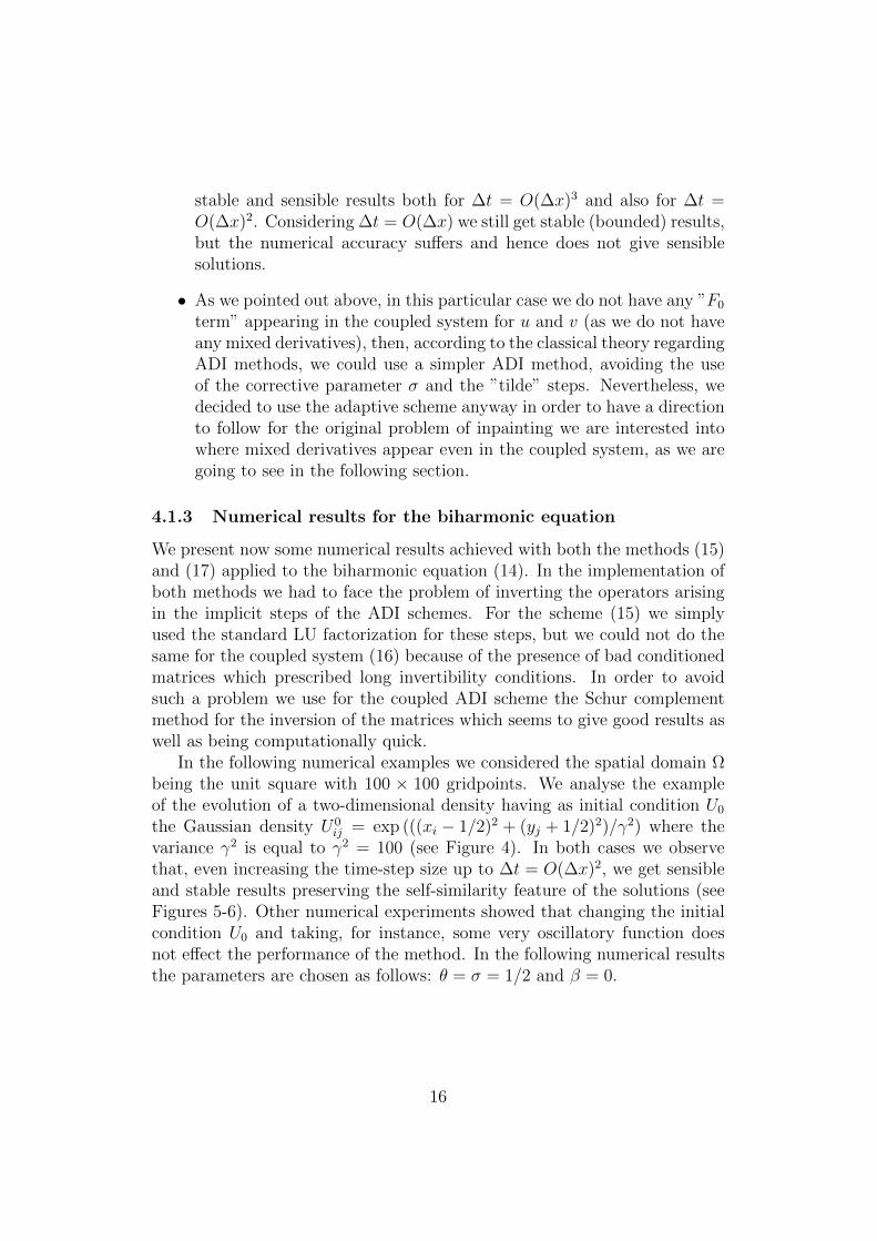
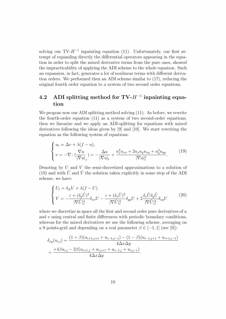
variance γ2 is equal to γ2 = 100 (see Figure 4). In both cases we observethat, even increasing the time-step size up to ∆t = O(∆x)2, we get sensibleand stable results preserving the self-similarity feature of the solutions (seeFigures 5-6). Other numerical experiments showed that changing the initialcondition U0 and taking, for instance, some very oscillatory function doesnot effect the performance of the method. In the following numerical resultsthe parameters are chosen as follows: θ = σ = 1/2 and β = 0.
16
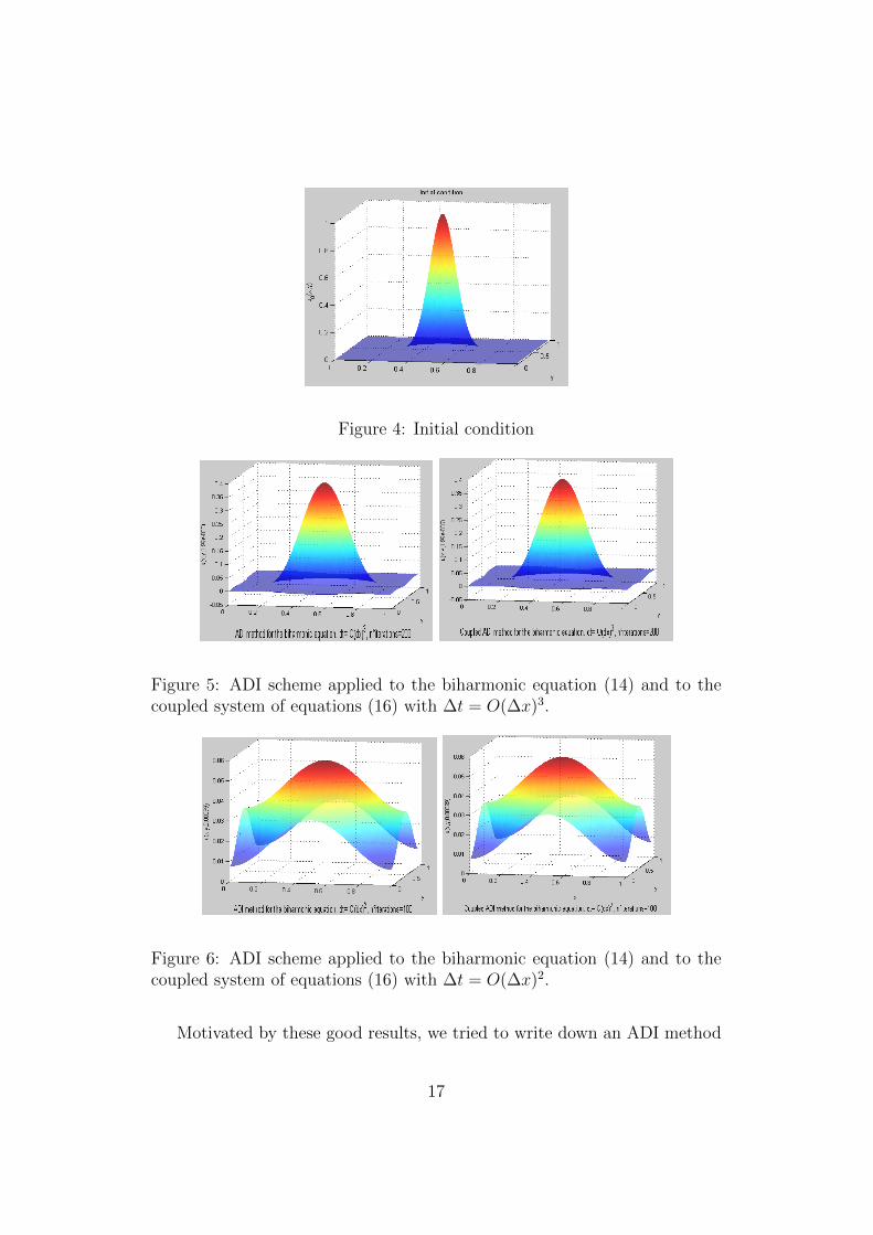
Figure 4: Initial condition
Figure 5: ADI scheme applied to the biharmonic equation (14) and to thecoupled system of equations (16) with ∆t = O(∆x)3.
Figure 6: ADI scheme applied to the biharmonic equation (14) and to thecoupled system of equations (16) with ∆t = O(∆x)2.
Motivated by these good results, we tried to write down an ADI method
17
solving our TV-H−1 inpainting equation (11). Unfortunately, our first at-tempt of expanding directly the differential operators appearing in the equa-tion in order to split the mixed derivative terms from the pure ones, showedthe impracticability of applying the ADI scheme to the whole equation. Suchan expansion, in fact, generates a lot of nonlinear terms with different deriva-tion orders. We performed then an ADI scheme similar to (17), reducing theoriginal fourth order equation to a system of two second order equations.
4.2 ADI splitting method for TV-H−1 inpainting equa-tion
We propose now our ADI splitting method solving (11). As before, we rewritethe fourth-order equation (11) as a system of two second-order equations,then we linearize and we apply an ADI-splitting for equations with mixedderivatives following the ideas given by [9] and [10]. We start rewriting theequation as the following system of equations:
ut = ∆v + λ(f − u),
v = −∇ · ( ∇u|∇u| ε
) = − ∆u
|∇u|ε+u2xuxx + 2uxuyuxy + u2
yuyy
|∇u|3ε.
(19)
Denoting by U and V the semi-discretized approximations to a solution of(19) and with U and V the solution taken explicitly in some step of the ADIscheme, we have:
Ut = δ∆V + λ(f − U)
V = −ε+ (δyU)2
|∇U |3εδxxU −
ε+ (δxU)2
|∇U |3εδyyU + 2
δxUδyU
|∇U |3εδxyU
(20)
where we discretize in space all the first and second order pure derivatives of uand v using central and finite differences with periodic boundary conditions,whereas for the mixed derivatives we use the following scheme, averaging ona 9 points-grid and depending on a real parameter β ∈ [−1, 1] (see [9]):
δxy(ui,j) =(1 + β)(ui+1,j+1 + ui−1,j−1)− (1− β)(ui−1,j+1 + ui+1,j−1)
4∆x∆y
++4βui,j − 2β(ui+1,j + ui,j+1 + ui−1,j + ui,j−1)
4∆x∆y.
18
4.2.1 The splitting of the operator
We write now the system (20) in the following matricial form:(UtV
)= F (U, V ) =
(A BC D
)·(UV
)+
(ST
)for suitable matrices A,B,C,D, S and T in RNM×NM . We split now F intothe sum of three different terms: F0 containing the mixed derivative termand F1 and F2 which contain the derivatives with respect to x and to y only,respectively. This produces the splitting:
F (U, V ) = F0(U, V ) + F1(U, V ) + F2(U, V ) (21)
with:
F0(U, V ) =
(A0 B0
C0 D0
)·(UV
)+
(ST
)=(
−Λ/3 0
2 δxUδyU|∇U |3εδxy 0
)·(UV
)+
(Λf
0
),
F1(U, V ) =
(A1 B1
C1 D1
)·(UV
)=
(−Λ/3 δxx
− ε+(δyU)2
|∇U |3εδxx 0
)·(UV
),
F2(U, V ) =
(A2 B2
C2 D2
)·(UV
)=
(−Λ/3 δyy
− ε+(δxU)2
|∇U |3εδyy 0
)·(UV
).
where Λ and Λf are suitable matrices in RNM×NM related to the fidelityterm, then containing the information on the region to inpaint. The idea ofsplitting Λ in three parts, one explicit and two implicit, seems to get goodnumerical results. An alternative could be splitting it between A1 and A2.For stability reason, it does not seem good putting the whole Λ in the explicitmatrix A0.
Finally, regarding the notations, for every Fj, j = 0, 1, 2, we will indicatethe rows of the respective coefficient matrix as follows:
Fj(U, V ) =
(F 1j (U, V )F 2j (U, V )
)
and we do the same for every vector Y =
(Y 1
Y 2
).
19

4.2.2 The ADI scheme
Given an initial condition (U0, V0) our problem consists in finding an approx-imation (Un+1, Vn+1) of the solution (u(tn+1), v(tn+1)) where tn = n∆t, n ≥ 1of (19). Now, setting (U , V ) = (Un, Vn), we present an ADI scheme to com-pute these approximations:
(Y 2
0
Y 10
)=
(F 2(Un, Vn)
Un + ∆tF 1(Un, Y2
0 ))
),(
Y 11
Y 21
)=
(Y 1
0
Vn
)+
(θ∆t(F 1
1 (Y 11 , Y
21 )− F 1
1 (Un, Vn))F 2
1 (Y 11 , Y
21 )− F 2
1 (Un, Vn)
),(
Y 12
Y 22
)=
(Y 1
1
Vn
)+
(θ∆t(F 1
2 (Y 12 , Y
22 )− F 1
2 (Un, Vn))F 2
2 (Y 12 , Y
22 )− F 2
2 (Un, Vn)
),(
Y 20
Y 10
)=
(F 2(Y 1
2 , Y2
2 )
Y 10 + σ∆t(F 1(Y 1
2 , Y2
0 )− F 1(Un, Vn))
),(
Y 11
Y 21
)=
(Y 1
0
Y 22
)+
(θ∆t(F 1
1 (Y 11 , Y
21 )− F 1
1 (Y 12 , Y
22 ))
F 21 (Y 1
1 , Y2
1 )− F 21 (Y 1
2 , Y2
2 )
),(
Un+1
Vn+1
)=
(Y 1
1
Y 22
)+
(θ∆t(F 1
2 (Y 12 , Y
22 )− F 1
2 (Y 12 , Y
22 ))
F 22 (Y 1
2 , Y2
2 )− F 22 (Y 1
2 , Y2
2 )
).
(22)
We briefly comment this elaborated scheme noting that, as in (17), thereare only two computations in the previous algorithm which are explicit time-steps: the first one and the fourth one where we take care of the mixedderivative terms of the problem. Once again in them the order of applicationof the method is reversed for consistency reasons, as pointed out previouslyfor the biharmonic equation. The other computations are implicit time-steps and, recalling the splitting given by (21), they break down the originalproblem acting once again just along one direction. Namely, the second andthe fifth computation of the scheme take care of the pure x− derivatives, thethird and the sixth one take care of the pure y− derivatives. Moreover weremark that, for consistency reasons, in the explicit steps we could not usethe approximations of Un+1 and Vn+1 given by the explicit steps. Namely,in the second and the third steps, for the approximations of Y 2
1 and Y 22 we
had to use just the value Vn (not the values Y 20 and Y 2
1 , respectively) andsimilarly for Y 2
1 and Vn+1.From a numerical point of view we just emphasize again that the inversion
of the operators in the implicit steps was performed again by using the Schurcomplement technique.
20

4.2.3 The choice of the linearization
In this subsection we want to explain why the choice of the linearization fromwhich our ADI scheme arises turns out to be important to get good results.Heuristically, such a choice is important from two different points of view,intrinsically related to each other. The former is the accuracy of the schemewe are considering: rough linearizations (i.e. linearizations which considermost of the nonlinear terms explicitly evaluating them in one or more givenapproximation) are likely to present poor accuracy as well as stability issuesarising from the explicit evaluation of the nonlinear and stiff terms. Thisis general consideration in the numerical solution of each partial differentialequation and, of course, it must be taken into account and balanced with thechoice of linearizations which might be more accurate and precise, but whichcould present, on the other hand, difficulties in their implementation andapplication. The latter point of view is, in some sense, peculiar to our choiceof performing a dimensional splitting scheme. As pointed out more thanonce above, in fact, our purpose is splitting our partial differential operatorinto the sum of components which are considered both explicitly (see F0
above) and implicitly (see F1 and F2). The choice of the linearization affectsthe splitting from two points of view: the operators we want to put in theexplicit component of F depend, in fact, from the linearization itself as wellas the quantities multiplying the differential operators considered implicitly,which play the role of coefficients (as they are given). Stability considerationsare, even from this point of view, very important and are strictly related thento the choice of the linearization.
In the following, we will make more precise our considerations and choices,analyzing in detail the linearization performed in (20) and showing howthings change when performing a different choice.
The first choice
We give now some motivations to the linearization performed in (20),pointing out some details. In the expression for v found in (19), obtainedby expanding fully the total variation term, the first choice we tried wasa rather accurate linearization where we decided to consider explicitly thenonlinear term |∇u|ε in the denominator and the derivatives of order one(and their powers) in the numerator, thus finding the approximation givenin (20) which, after discretizing also in time, can be more precisely writtenas:
21
Un+1 − Un
∆t= ∆V n+1 + λ(f − Un+1)
V n+1 = −ε+ (δyUn)2
|∇Un|3εδxxU
n+1 − ε+ (δxUn)2
|∇Un|3εδyyU
n+1 + 2δxU
nδyUn
|∇Un|3εδxyU
n+1
(23)for every n ≥ 0. The disadvantage of performing such an accurate choice,
is the appearing of the mixed derivative term with all the related problemswe have already discussed above. Nonetheless, it is hoped the accuracy ofthis linearization can have a better performance than more brutal ones.
The second choice
Another possibility is linearizing the system (19) in a an apparently moreinaccurate way, though with some advantages from the point of view of ourADI numerical scheme. The alternative is the following:
Un+1 − Un
∆t= ∆V n+1 + λ(f − Un+1),
V n+1 = −∇ · (∇Un+1
|∇Un| ε) = − 1
|∇Un|εδxxU
n+1 +UnxU
nxx + Un
y Unxy
|∇Un|3εδxU
n+1
− 1
|∇Un|εδyyU
n+1 +UnxU
nxy + Un
y Unyy
|∇Un|3εδyU
n+1.
(24)We observe that with such a choice we do not have anymore the mixed
derivative operator acting on Un+1 because the mixed terms are encodedand considered in the previous time step. On the other hand, we get firstderivative operators and not just second order ones as in (23). Namely, weare still considering the splitting the operator given by:
F (U, V ) = F0(U, V ) + F1(U, V ) + F2(U, V )
but this time the choice is:
F0(U, V ) =
(−Λ/3 0
0 0
)·(UV
)+
(Λf
0
),
F1(U, V ) =
(−Λ/3 δxx
− 1|∇Un|ε δxx +
Unx U
nxx+Un
y Unxy
|∇Un|3εδx 0
)·(UV
),
F2(U, V ) =
(−Λ/3 δyy
− 1|∇Un|ε δyy +
Unx U
nxy+Un
y Unyy
|∇Un|3εδy 0
)·(UV
)
22

where we have used the same notation as above. The resulting scheme hasthe same structure as in (22), but with the different choice of the functionspointed out above. The balance between the predicted improvements in thestability behaviour giving by the absence of the explicit mixed derivativeoperator and the issues related to too rough-linearization seems to indicate agenerical bad instability tendency with blowing up the numerical solutions.
The third choice
Another possible alternative to the linearization is exploiting the so-calledprimal-dual formulation of the problem (11) and adding a penalty or bareerterm as suggested in [1] and [12]...
4.2.4 Numerical results
We present now some numerical results obtained applying the scheme (22)to our inpainting equation (11). In order to study the properties of thenumerical scheme we first applied it to the equation taking λ = 0, i.e. we juststudied the evolution of the nonlinear process without the fidelity inpaintingterm for a given initial datum. What we expect for such an equation is abetter edge-preserving behaviour than the one showed by the biharmonicequation as the term ∇ · ( ∇u|∇u|ε ) is the subgradient of to the total variation
and as such reduces diffusion in areas of large image gradient (i.e. of edges).The approximation parameter ε becomes then a ”measure” of how close thenonlinear process is to the biharmonic one. Big values of ε should in fact showbehaviours similar to the smoothing effect of the biharmonic equation (asε increases the denominator |∇u|ε becomes infinitely large), whereas smallvalues of ε should show edge-preserving features, typical of total-variationmethods. The results we got seem instead to show a better (and stable)behaviour for big values of ε, according also to the size of the time-step sizeconsidered. We tested also the stability of the scheme and the results givenfor different ε when considering different, typically more oscillatory, initialconditions, thus finding that the stability properties of such a scheme seemto depend also on the variations of the gradient of the initial condition: veryoscillatory initial conditions with really steep gradients will present harderstability constraints on the time step and require then bigger values of ε.The analytical and precise reasons for that has still to be explored and it isa matter of future research.
In the following we present first the results we get by the application ofthe scheme (22) to the nonlinear equation (11) with the choice λ = 0. Thedifferent choices of the regularizing parameter ε are written gradually. Weconsider at first the same initial condition as before, changing it with the
23

more oscillatory function u0(x, y) = sin(15x) + cos(15y). We include herethe results obtained taking time-step sizes equal to ∆t = O(∆x)3 and ∆t =O(∆x)2 as they appear more interesting from a computational point of viewbecause, as we have said before, they overcome the prohibitive constraint∆t = O(∆x)4 to solve our original inpainting problem.
(a) Gaussian initial con-dition.
(b) Oscillatory initialcondition.
Figure 7: Initial conditions
(a) Gaussian datum. (b) Oscillatory datum.
Figure 8: Result ε = 100 and ∆t = O(∆x)3 for the two different initialconditions after 200 iterations.
24

(a) Gaussian datum. (b) Oscillatory datum.
Figure 9: Result with ε = 1000 and ∆t = O(∆x)3 for the two different initialconditions after 200 iterations.
(a) Gaussian datum. (b) Oscillatory datum.
Figure 10: Unstable results with ε = 1 and ∆t = O(∆x)3 for the two differentinitial conditions after few iterations.
(a) Gaussian datum. (b) Oscillatory datum.
Figure 11: Results with ε = 100 and ∆t = O(∆x)2 for the two differentinitial conditions after 100 and 3 iterations.
25

(a) Gaussian datum. (b) Oscillatory datum.
Figure 12: Results with ε = 1000 and ∆t = O(∆x)2 for the two differentinitial conditions after 100 and 13 iterations.
(a) Gaussian datum. (b) Oscillatory datum.
Figure 13: Results with ε = 104 and ∆t = O(∆x)2 for the two differentinitial conditions after 100 iterations.
4.2.5 Numerical results applied to TV-H−1 inpainting
We conclude this report presenting in the following figures some numericalresults obtained applying the ADI method (22) presented above. For thesake of simplicity in the example below we have considered the square image(N = M) with dimension 100 × 100 pixels. Figures 14 and 15 show thebest results we can get (i.e. for sensible values of ε) in a reasonable amountof time for different time-step sizes. Figure 16 shows instead the behaviourof the method for different values of the tuning parameter λ. The stabilityproblems mentioned above still exist for the equation (11) and they do notseem to be overcome by changing the size of the fidelity parameter λ.
26

Figure 14: On the left: initial condition. On the right: result at time tn =9× 10⁻⁵ for ∆t = O(∆x)4, λ = 109 and ε = 0.1.
Figure 15: On the left: result at time tn = 5.5× 10⁻⁵ for ∆t = O(∆x)3, λ =109 and ε = 10. On the right: result at time tn = 0.0142 for ∆t = O(∆x)2,λ = 109 and ε = 100
Figure 16: On the left: result at time tn = 1 × 10⁻⁵ for ∆t = O(∆x)4,λ = 105 and ε = 0.01. On the right: result at time tn = 1.22 × 10⁻⁵ for∆t = O(∆x)3, λ = 105 and ε = 10. We observe that we get poor and ratherunstable results.
27
4.3 The ADI-Newton scheme
The second method we propose follows the ideas presented in [15] where,however, the authors deal with problems related to the study of lubrificationflows of thin liquid films and are able to approximate the mean curvature(i.e. the divergence term in the inpainting equation) by the Laplace operatorin the small gradient limit. We cannot perform such approximation any-more, since we are interested in looking at the variations of the image whenedges appear, that is when the values of the gradient are significantly large.Accurate numerical solutions of nonlinear problems generally necessitate theuse of iterative schemes like Newton’s method to calculate the approximatedsolution at the next time-step Un+1 given the solution at the previous time-steps Un, Un−1, . . . . Solving nonlinear problems like (11) using a backwardEuler scheme involves actually a combination of iterative processes:
1. The application of Newton’s method at each time step to find the so-lution of the discretized nonlinear problems (i.e. for every n we wantto find Un+1 such that for some F describing the problem we haveF (Un+1) = 0);
2. At each step of Newton’s method, some other iterative method mustbe used to solve large sparse linear algebra problem produced by thetwo-dimensional linearized operator, namely the Jacobian matrix whichappears in Newton’s method (i.e. we iterate the process according to
an index k in order to get approximations U(k)n+1 of Un+1).
We want to use some ADI scheme for the second process in order toreduce it to a direct solution of an approximately factored problem. Then,the iteration of 1. guarantees convergence to the solution3. We focus nowon the use of Newton’s method. Consider solving (11) directly, using abackward Euler method. At each time-step, the discretized problem requiresthe solution of the system of nonlinear equations given by
F (Un+1) := Un+1 − Un + ∆t∆∇ ·(∇Un+1
|∇Un+1|ε
)−∆tλ(f − Un+1) = 0
where the performed space discretizations will be specified later on. Theapplication of the Newton’s method to solve nonlinear system yields thefollowing iterative method:
J(U(k)n+1)v = −F (U
(k)n+1), v := U
(k+1)n+1 − U
(k)n+1, k = 0, 1, 2, · · · , (25)
3Some authors refer to this kind of method calling them iterative factorized methods.
28

where, by iterating the process, we find some approximation to the solutionat tn+1. At each time step we initially estimate Un+1 by the trivial explicit
first-order approximation U(0)n+1 = Un and then we keep iterating on k thus
finding better and better approximations of Un+1. According to the theory
regarding Newton’s methods we know that if U(0)n+1 is chosen to be sufficiently
close to Un+1, the sequenceU
(k)n+1
k
converges quadratically to Un+1.
Using now the shorthand U to indicate the quantity U(k)n+1 (”explicit” as
regarding the previous iteration on k), we write down the Jacobian (namely,the Frechet derivative) appearing in (25) by:
J(U)v ≡ δF
δUv =
d
dεF (U + εv)|ε=0 = ∆t∆[−∆U
∇U · ∇v|∇U |3ε
− 1
|∇U |3ε(∇U ·Hv∇U + 2∇U ·HU∇v) +
3
|∇U |5ε(∇U ·HU∇U)(∇U · ∇v)
(26)
+∆v
|∇U |ε] + (1 + λ)v
where we have indicated by HU and Hv the matrices:
HU =
((U)xx (U)xy(U)xy (U)yy
)Hv =
(vxx vxyvxy vyy
)Such approach can be computationally expensive and may become limitingin the speed and of numerical simulations for these problems. In order todevelop a more efficient approach, we consider an approximate Newton’smethod, where we approximate the Jacobian using the factorization J ≈LxLy with the following choice of the operators:
Lx = I + ∆tDx Ly = I + ∆tDy.
The differential operators Dx and Dy appearing in such a decompositionare obtained linearizing the quantity in the square brackets of (26) so that nomixed derivatives of v could appear. The idea exploited to do that is to con-sider for each operator just the terms involving effectively the ’corresponding’derivatives (for example, for Dx just the terms involving derivatives with re-spect to x) and to substitute the other quantities (for example, the derivativeswith respect to y) with the corresponding explicit term related to U . Actingin such a way, we add some further terms, but on the other hand we are ableto exploit the advantage of considering the ’one-dimensional’ operators given
29

by:
Dx(φ) = ∂xx[−∆UUxφx + U2
y
|∇U |3ε− 1
|∇U |3ε(U2
xφxx + φx(UxUxx + UxyUy)
+ 3UxUyUxy + 2U2y Uyy) +
3
|∇U |5ε(∇U ·HU∇U)(Uxφx + U2
y ) +φxx + Uyy
|∇U |ε
− 1
|∇U |3ε(φx(UxxUx + UxyUy) + UxUyUxy + U2
y Uyy)],
Dy(φ) = ∂yy[−∆UUyφy + U2
x
|∇U |3ε− 1
|∇U |3ε(2U2
x Uxx + φy(UxUxy + UyyUy)
+ 3UxUyUxy + U2yφyy) +
3
|∇U |5ε(∇U ·HU∇U)(U2
x + Uyφy) +Uxx + φyy
|∇U |ε
− 1
|∇U |3ε(U2
x Uxx + UxUxyUy + φy(UxyUx + UyyUy)]
With this choice of operators, we have the following ADI scheme, used inthe Newton method (25) to solve the method approximatively:
Lxw = −F (U(k)n+1),
Lyv = w
U(k+1)n+1 = U
(k)n+1 + v.
(27)
In the implementation of such a method we had to write down all theprevious (horrible) operators. In order to do that we used the followingdecomposition of the operators Dx and Dy:
Dx(φ) = Dx(φ) + g1(U) and Dy(φ) = Dy(φ) + g2(U) (28)
such that both the operators Dx and Dy act directly on φ via some dif-ferential operators (namely, taking x and y derivatives of φ multiplied for
some coefficients depending just on the value U = U(k)n+1 which is given in
the previous iteration) while the functions g1 and g2 contain all the givenquantities depending just on U and then they are not acting on the unknownφ. Using the same notation used in the code, the operators Dx and Dy and
30

the functions g1 and g2 turn out to be:
Dx(φ) = ∂xx[−∆U
|∇U |3εUxφx] + ∂xx[−
(Ux)2
|∇U |3εφxx] + ∂xx[−
2(UxUxx + UyUxy)
|∇U |3εφx]
+ ∂xx[3(∇U ·HU∇U)Ux
|∇U |5εφx] + ∂xx[
1
|∇U |εφxx]
= a1xxφx + 2a1xφxx + a1φxxx + a2xxφxx + 2a2xφxxx + a2φxxxx + a3xxφx + 2a3xφxx
+ a3φxxx + a4xxφx + 2a4xφxx + a4φxxx + a5xxφxx + 2a5xφxxx + a5φxxxx
= (a1xx + a3xx + a4xx)φx + (2a1x + a2xx + 2a3x + 2a4x + a5xx)φxx
+ (a1 + 2a2x + a3 + a4 + 2a5x)φxxx + (a2 + a5)φxxxx
Dy(φ) = ∂yy[−∆U
|∇U |3εUyφy] + ∂yy[−
(Uy)2
|∇U |3εφyy] + ∂yy[−
2(UyUyy + UxUxy)
|∇U |3εφy]
+ ∂yy[3(∇U ·HU∇U)Uy
|∇U |5εφy] + ∂yy[
1
|∇U |εφyy]
= b1yyφy + 2b1yφyy + b1φyyy + b2yyφyy + 2b2yφyy + b2φyyyy + b3yyφy + 2b3yφyy
+ b3φyyy + b4yyφy + 2b4yφyy + b4φyyy + b5yyφyy + 2b5yφyyy + b5φyyyy
= (b1yy + b3yy + b4yy)φy + (2b1y + b2yy + 2b3y + 2b4y + b5yy)φyy
+ (b1 + 2b2y + b3 + b4 + 2b5y)φyyy + (b2 + b5)φyyyy
g1(U) = ∂xx(−∆U
|∇U |3ε(Uy)
2) + ∂xx(−1
|∇U |3ε(3UxUyUxy + 2(Uy)
2Uyy))
+ ∂xx(3
|∇U |5ε(∇U ·HU∇U)(Uy)
2) + ∂xx(Uyy
|∇U |ε)
+ ∂xx(−1
|∇U |3ε(UxUyUxy + Uyy(Uy)
2) = ∂xxt1 + ∂xxt2 + ∂xxt3 + ∂xxt4 + ∂xxt5
g2(U) = ∂yy(−∆U
|∇U |3ε(Ux)
2) + ∂yy(−1
|∇U |3ε(3UxUyUxy + 2(Ux)
2Uxx))
+ ∂yy(3
|∇U |5ε(∇U ·HU∇U)(Ux)
2) + ∂yy(Uxx
|∇U |ε)
+ ∂yy(−1
|∇U |3ε(UxUyUxy + Uxx(Ux)
2) = ∂yys1 + ∂yys2 + ∂yys3 + ∂yys4 + ∂yys5.
The coefficients ai and bi are nothing but the terms into the square brack-ets which depend just on U , then they are ’given’ and they don’t act directly
31

on φ. The expressions above have been found by simply applying the Leibnizformula for products of functions. We can observe then that each differen-tial operator Dx and Dy acts just on the corresponding derivatives of thefunction to which it is applied: no mixed derivatives appear and the nonlin-earities appearing in (11) are overcome by considering all the terms derivingfrom them explicitly, by the linearization described above.
As far as the spatial discretizations are concerned, we point out that weused for each operator different ”stencils” of grid points on which we aver-aged to find the approximation of the derivatives. Namely we used 9-pointgrid stencil for the first and the second derivatives, and the 25-point one forthe third and the fourth derivatives, then assembling everything together.Namely, we discretized the x-derivatives of ui,j, where the couple i, j repre-sents a pixel in the image as:
δcx(ui,j) =ui+1,j − ui−1,j
2∆x
δxx(ui,j) =ui+1,j − ui−1,j − 2ui,j
∆x2
δxxx(ui,j) = δcx(δxx(ui,j)) =ui+1,j − 2ui+1,j + 2ui−1,j − ui−2,j
2∆x3
δxxxx(ui,j) = δxx(δxx(ui,j)) =ui+2,j − 4ui+1,j + 6ui,j − 4ui−1,j + ui−2,j
∆x4
and similarly for the y-derivatives.By construction we see that this method turns out to be a semi-implicit
method, i.e. some parts of the equation are taken explicitly (introduced bythe Newton approximation and the dimensional splitting), some implicit intime. Hence, the stability of such a strategy becomes an important consid-eration and has still to be explored. However, we point out that differentlyfrom the second method we are about to present in the next section, in thisADI-Newton method there are no solutions of explicit in time-steps involved.
Even though from a theoretical point of view the ADI-Newton methodpresented above seems to be very promising, its implementation gave us someproblems we were not able to fix. The main problem we experienced was thebad conditioning behaviour of the large and sparse matrices representing theoperators Lx and Ly which caused issues in the inversion of such operatorsin the steps of (27). A fist attempt could be using some preconditioningmethod to overcome this problem or finding some other approximation ofthe Jacobian J different from the ”factorized” one presented above.
32
5 Appendices
We recall now some mathematical concepts which have been useful in ouranalysis. In all this section we will indicate with Ω an open and boundeddomain in R2 with Lipschitz boundary Γ := ∂Ω.
A The space H−1
We define the non-standard Hilbert space H−1(Ω) as:
H−1(Ω) :=F ∈ H1(Ω)∗ : H1(Ω)∗〈F, 1〉H1(Ω) = 0
.
The norm of a function F ∈ H−1(Ω) is defined as
‖F‖2−1 :=
∥∥∇∆−1F∥∥2
L2(Ω)=
∫Ω
(∇∆−1F (x))2dx
where the operator ∆−1 denotes the inverse of the Laplacian with Neumannboundary conditions, i.e. u := ∆−1F is the unique weak solution in the spaceH1N(Ω) :=
ψ ∈ H1(Ω) :
∫Ωψ(x)dx = 0
of the problem:
∆u = F in Ω
∇u · ν = 0 on Γ
where ν denote the outward normal vector on Γ. For further characterizationsof this space we refer to [4, Appendix A].
B Functions of bounded variation
We define the space of functions of bounded variation BV (Ω) in bidimen-sional domain as follows:
Definition B.1 (BV (Ω). Let u ∈ L1(Ω). We say that u is a function ofbounded variation in Ω if the distributional derivative of u is representableby a finite Radon measure in Ω, i.e. if:∫
Ω
u(x)∂φ
∂xi(x)dx = −
∫Ω
φ(x)dDiu(x) = 〈u′, φ〉L2(Ω) ∀φ ∈ C∞c (Ω), i = 1, 2
for some R2-valued measure Du = (D1u,D2u) in Ω. We denote the vectorspace of all such functions by BV (Ω).
33

It is possible to characterize the space BV (Ω) by the total variation ofDu. Before doing it we define the variation of a function in L1
loc(Ω) and thetotal variation of a measure.
Definition B.2 (Variation). Let u ∈ L1loc(Ω). The variation V (u,Ω) of u
in Ω is defined by:∫Ω
|Du| := sup
∫Ω
u(x)∇ · φ(x)dx : φ ∈ (C1c (Ω))2, ‖φ‖∞ ≤ 1
.
We point out that just integrating by parts we see that∫
Ω|Du| =
∫Ω|∇u(x)|dx
if u ∈ C1(Ω) and, using density argument, the same holds for functions inW 1,1(Ω).
Definition B.3 (Total variation). Let (X, E) be a measure space. If µ is ameasure, we define for every E ∈ E its total variation |µ| as follows:
|µ|(E) := sup
∞∑n=0
|µ(En)| : En ∈ E , Ei ∩ Ej = ∅ ∀i 6= j, E =∞⋃n=0
En
.
With the previous definitions we can characterize the space BV (Ω) withthe following theorem.
Theorem B.4 (Characterization of BV (Ω)). Let u ∈ L1(Ω). Then, u ∈BV (Ω) if and only if
∫Ω|Du| <∞. Moreover,
∫Ω|Du| coincides with |Du|(Ω)
for any u ∈ BV (Ω) and the map:
T : u 7→ |Du|(Ω)
is lower semicontinuous in BV (Ω) with respect to the L1loc(Ω) topology.
We also recall that BV (Ω) is a Banach space endowed with the norm:
‖u‖BV (Ω) := ‖u‖L1(Ω) +
∫Ω
|Du|.
Moreover, we point out that BV (Ω) is continuously embedded in L2(Ω) if,as in our case, Ω ⊂ R2.
C Frechet derivatives and subdifferentials
Definition C.1 (Frechet differentiability). Let H be a Hilbert space withnorm ‖·‖ and inner product (·, ·) and let E : H → R. Given u ∈ H we saythat E is Frechet differentiable at u if there exists ξ ∈ H such that:
lim‖v‖→0
E(u+ v)− E(u)− (ξ, v)
‖v‖= 0.
34

The element ξ is necessarily unique and it is called the Frechet derivativeof E at u or the first variation of E at u. We will indicate such ξ with δE.
When the limit does not exist we can define a suitable generalizationintroducing the notion of subdifferential of a convex function.
Definition C.2 (Subdifferential). Let X be a locally convex space, let X∗ beits dual and 〈·, ·〉 the duality pairing X∗ −X. Given a convex map F of Xinto R, we define the subidifferential of F at u ∈ X as:
∂F (u) := ξ ∈ X∗ : 〈ξ, v − u〉 ≤ F (v)− F (u) ∀v ∈ X .
Since every normed vector space is locally convex, we can therefore applythe theory of subdifferentials in the framework of the functions of boundedvariation introduced above. For further details see [8].
Acknowledgements
I am deeply and sincerely grateful to Carola Schonlieb for all the discussionswe had and for all the time I took her up to realize this project. Thanks toher, I was introduced to the exciting area of image processing which I reallywould like to deepen in the future.
References
[1] M. Benning, Singular regularization of inverse problems, 2011.
[2] M. Bertalmio, G. Sapiro, V. Caselles, C. Ballester, Image inpainting,Siggraph 2000, Computer Graphics Proceedings, 417-424, 2000.
[3] A. Bertozzi, S. Esedoglu, A. Gillette, Inpainting of binary images usingthe Cahn-Hilliard Equation, IEEE Trans. Image Proc., 16 (1), 285-291,2007.
[4] M. Burger, L.He, C.-B. Schonlieb, Cahn-Hilliard inpainting and a gen-eralization for grayvalue images, SIAM J. Imaging Sci., 2 (4), 1129-1167,2009.
[5] T.F. Chan, J. Shen, Variational image inpainting, Commun. Pure Ap-plied Math., 58, 579-619, 2005.
[6] B. During, C. B. Schonlieb, A high-contrast fourth-order PDE fromimaging: numerical solution by ADI splitting, to appear.
35

[7] D. Eyre, An unconditionally stable One-Step Scheme for Gradient Sys-tems, unpublished, 1998.
[8] L. C. Evans, Partial differential equations, Graduate Studies in Mathe-matics 19, American Mathematical Society, Providence, RI, 2010.
[9] K.J. in ’t Hout, B.D. Welfert, Stability of ADI schemes applied toconvection-diffusion equations with mixed derivative terms, Appl. Nu-mer. Math., 57, 19-35, 2007.
[10] K.J. in ’t Hout, B.D. Welfert, Unconditional stability of second-orderADI schemes appliet to multi-dimensional diffusion equations with mixedderivative terms, Appl. Numer. Math., 59, 677-692, 2009.
[11] W. Hundsdorfer, J.G. Verwer, Numerical solution of time-dependentadvection-diffusion-reaction equations, Berlin: Springer-Verlag, 2003.
[12] J. P. Muller, Parallel total tariation minimization, Diploma thesis,Munster, November 2008.
[13] C.B. Schonlieb, A. Bertozzi, Unconditionally stable schemes for higherorder inpainting, Commun. Math. Sci., 9 (2), 413-457, 2011.
[14] A. M. Stuart, A. R. Humphries, Model problems in numerical stabilitytheory for initial value problems., SIAM Rev. 36, 226-257, 1994.
[15] T.P. Witelski, M. Bowen ADI schemes for higher-order nonlinear diffu-sion equations, Appl. Numer. Math., 45, 331-351, (2003).
36