Journal of Applied Mathematics and Physics, 2016, 4, 1600-1609 Published Online August 2016 in SciRes. http://www.scirp.org/journal/jamp http://dx.doi.org/10.4236/jamp.2016.48170

How to cite this paper: Lin, B. (2016) Spline Solution for the Nonlinear Schrödinger Equation. Journal of Applied Mathe-matics and Physics, 4, 1600-1609. http://dx.doi.org/10.4236/jamp.2016.48170

Spline Solution for the Nonlinear Schrödinger Equation Bin Lin School of Mathematics and Computation Science, Lingnan Normal University, Zhanjiang, China

Received 13 July 2016; accepted 22 August 2016; published 25 August 2016

Copyright © 2016 by author and Scientific Research Publishing Inc. This work is licensed under the Creative Commons Attribution International License (CC BY). http://creativecommons.org/licenses/by/4.0/

Abstract We develop an exponential spline interpolation method to solve the nonlinear Schrödinger equa-tion. The truncation error and stability analysis of the method are investigated and the method is shown to be unconditionally stable. The conservation quantities are computed to determine the conservation properties of the problem. We will describe the method and present numerical tests by two problems. The numerical simulations results demonstrate the well performance of the proposed method.

Keywords Nonlinear Schrödinger Equation, Exponential Spline Interpolation, Gross-Pitaevskii Equation, Mass and Energy Conservation

1. Introduction Consider the following nonlinear Schrödinger equation

( )21 2 , 0,t xxmu u u u x t uλ λ ε+ + + = (1)

With the boundary conditions

( ) ( ) ( ) ( )1 2, , , , 0u c t t u d t t tβ β= = ≥ (2)

And the initial condition

( ) ( )0, 0 , ,u x u x x= ∈ (3)

where 1m = − , ( ),u x t is the complex-valued wave function. 1λ and 2λ are constant, ( ),x tε is a

B. Lin

1601

bounded real function. This equation plays important roles in nonlinear physics. It can describe many nonlinear phenomena including plasma physics [1], hydrodynamics [1] [2], self-focusing in laser pulses [3], propagation of heat pulses in crystals, models of protein dynamics [4], quantum mechanics [5], models of energy transfer in molecular systems [6] and quantum mechanics and optical communication [7]-[9] and so on.

In the past few years a great deal of efforts has been expended to solve NLS equations. It is more difficult to find the analytical solutions of the NLS equation, so the study of the numerical solution of NLS equation in the theory and application is important. Its numerical solutions have been researched by many authors. For example, finite difference method [10] [11], quasi-interpolation scheme [12], quadratic B-spline finite element scheme [13], compact split-step finite difference method and pseudo-spectral collocation method [14] [15], exponential spline method [16], spline methods [17] [18], split-step orthogonal spline collocation method [19], a high-order and accurate method [20], linearly implicit conservative scheme [21].

The aim of this paper is to give an exponential spline interpolation method for the NLS equation. The paper is organized as follows. In Section 2, construction of the method is presented. The stability analysis of the scheme is investigated in Section 3. In Section 4, the computation of conserved quantities and error norms are given. In Section 5, two numerical examples are presented to demonstrate our theoretical results. The last section is a brief conclusion.

2. Construction of Exponential Spline Interpolation Method We set up a grid in the ,x t plane with grid points ( ),i jx t and uniform grid spacing h and k, where

1 1, , 0,1, 2, ,i i i ix a ih h x x i N+ += + = − = and , 0,1, 2,jt jk j= = . In the interval [ ]1,i ix x + , a exponential spline function ( ),i jS x t is given by

( ) ( ) ( ) ( )1 2 3 4, ,j j j ji j i i i i i i i i iS x t c c x x c x x c x xψ φ= + − + − + − (4)

where 1 2 3 4, , ,i i i ic c c c are coefficients to be determined, iψ and iφ are the auxiliary functions which contain a stiffness parameter 1ip + which will be used to raise the accuracy of the method, on the support [ ]1,i ix x + and are given by

( ) ( )( ) 21 12 cosh 1 ,i i i ix p x x pψ + + = − − (5)

( ) ( )( ) ( ) 21 1 16 sinh ,i i i i i ix p x x p x x pφ + + + = − − − (6)

Since the Taylor series expansions of the hyperbolic functions are

( ) ( ) ( )3 5

sinh ,3! 5!px px

px px= + + + (7)

( ) ( ) ( )2 4

cosh 1 ,2! 4!

px pxpx = + + + (8)

We note that iψ and iφ tend to ( )2ix x− and ( )3

ix x− in the limit of p tending to zero, and in the op-posite limit of p tending to infinity the nonlinear terms in iψ and iφ vanish as 1 p .

So the exponential spline defined above share a number of interesting properties: (1) When 0p → , ( ),i jS x t reduces to cubic spline; when p →∞ , ( ),i jS x t reduces to linear spline. (2) A change of character of the exponential spline function is from linear to third order polynomial on adja-

cent support intervals. (3) In the general case the stiffness parameters p are different on every interval which provides the extremely

high flexibility of the exponential spline function. We wish to find j

nic in Equation (4), 1, 2,3, 4n = , Letting ( ) ( )2 ,ji jM S x t∆= be the unknown second deriva-

tive of the exponential spline of interpolation at the grid points, we can obtain the following representation for ( ), jS x t∆ on [ ]1,i ix x + in terms of the known interpolation data 1,j j

i iu u + and the unknown spline second de-rivatives 1,j j

i iM M +

B. Lin

1602

( ) ( )( )( )( )

( )( )( )( ) [ ]

1 11 11 2

1 1 11 1 1

1112

11 1 1

sinh,

sinh

sinh, , ,

sinh

ji ij ji i i i

j i ii i i i i ii i i i

ji ii i

i ii ii i i i

p x xx x x x M x xS x t u ux x x x x xp p x x

p x xM x x x x xx xp p x x

+ ++ +∆ +

+ + ++ + +

+++

++ + +

−− − −= + − −

− − −− − −

+ − ∈ −−

(9)

The terms involving the values jiu and 1

jiu + represent the linear interpolation part of ( ), jS x t∆ . The terms

involving the second derivatives jiM and 1

jiM + introduce the curvature.

The function ( ), jS x t∆ on the interval [ ]1,i ix x− is obtained with 1i − replacing i in Equation (9). The continuity requirement for the first derivative ( ) ( )1 , jS x t∆ at the point ix yields the following equation:

( ) 1 11 1 1 1

1

,j j j j

j j j i i i ii i i i i i i

i i

u u u uA M B B M A Mh h+ −

− + + ++

− −+ + + = − (10)

where ( )( )

( ) ( )( )2 2

sinh cosh sinh, ,

sinh sinhi i i i i i i i i i

i i i ii i i i i i

p h p h p h p h p hA h B h

p p h p p h− −

= =

Remark 1. (1) By expanding Equation (10) in Taylor series, the truncation error for Equation (10) is of the form

( )

( ) ( ) ( ) ( )

( ) ( ) ( )

2 2 21 11 1 1 1

1

21 1 2 1 3

2 33 2 4 3

1 4 1

1 12 6

1 112 2 20

j j j jj j j ji i i i

i i x i i i x i i x ii i

j ji ii i i i i x i i i i i xi i

ji i i ii i i i x i i i ii

u u u uT A D u B B D u A D uh h

h hA A B B u A A h u

h h h hA A u A A

σ σ σ

σ σ σ σ

+ −− + + +

+

+ + +

+ +

− −= − − − + −

= + − − − − + − + −

+ + − − + − + − ( )

( ) ( ) ( )

5

45 4 5

1 6

6

1 ,30 24

jx i

ji ii i i i x ii

u

h hA A u O hσ σ+ + + − − +

(11)

where 1 1 1,i i i i i ih h h x xσ + + += = − .

For ( ) ( )2 211 , 1

12 12i i i i i ii

h hA Aσ σ σ σσ+= − + + = + − , ( )3 2

1 4 4 112

ii i i i i

i

hB B σ σ σσ++ = + + + , the truncation

error in space of the relation (10) is of ( )4O h . From Equation (10), we can obtain

( ) ( )1 11 1 1 1

1,

j j ji i i i ij j j

i i i i i i ii i

u u uA M B B M A M

hσ σ

σ− +

− + + +

− + ++ + + = (12)

Or

( ) ( )1 1 1

1 1 1 2 2 21 12 2 2

1 1 1 11

,j j j

j j j i i i i ii i i i i i i

i i

u u uA M B B M A M

hσ σ

σ

+ + ++ + + − +− + + +

− + ++ + + = (13)

Further, when 1iσ = , then 1i ih h h += = , 1 110,

12 12i i i ih hA A B B+ += = + = , the truncation error in space of the

relation (10) is of ( )5O h , Equation (2.7) can be rewritten as

( )1 1 1 121210 2 ,j j j j j j

i i i i i iM M M u u uh+ − + −+ + = − + (14)

1 1 1 1 1 12 2 2 2 2 2

1 1 1 121210 2 ,

j j j j j j

i i i i i iM M M u u uh

+ + + + + +

+ − + −

+ + = − +

(15)

In order to get the error estimates of Equation (10), we put ehDE = in Equation (12), where E and D are the

B. Lin

1603

shift and differential operators respectively, and expand them in powers of hD, we have

( ) ( )1

42 1

12 2 , , 1, 2, , .10

j ji i xx i j

E I EM u u x t O h i Nh E I E

−

−

− += = + =

+ + (16)

Or

( ) ( )4 , 1, 2, , .j jxx ii

u M O h i N= + = (17)

At the grid point ( ),i jx t , Equation (1) can be discretized by

( ) ( )2 211 1 11 1

22 2 221 2 0,2

j jj j j j jj i ii ixx i i ii

u uu um u u u O kk

λ ε λ++ + + ++ +−

+ + + + = (18)

From Equation (18), we have

( )2 211 1 11

1 1 21 12 2 21 1 2 1

1 1

1 ,2

j jj jj j ji ii ii i i

u uu uM m u O kk

ε λλ λ

+++ + +− −− −− − −

+− = − − + +

(19)

( )2 211 1 11

22 2 22

1 1

1 ,2

j jj jj j ji ii ii i i

u uu uM m u O kk

ε λλ λ

+++ + + +− = − − + +

(20)

( )2 211 1 11

1 1 21 12 2 21 1 2 1

1 1

1 ,2

j jj jj j ji ii ii i i

u uu uM m u O kk

ε λλ λ

+++ + ++ ++ ++ + +

+− = − − + +

(21)

Substituting Equation (19), Equation (20) and Equation (21) into Equation (15) and after some simplifications, we obtain

1 1 1 * * *1 1 2 3 1 1 1 2 3 1

j j j j j ji i i i i i i i i i i iF u F u F u F u F u F u+ + +

− + − ++ + = + + (22)

where 2 211

221, 2, , , 1, 2, , ,

2

j jj i ij

i i

u ui N j δ ε λ

++ +

= = = +

( ) ( )

( ) ( )

( ) ( )

11 1 22

1 1

*13 1 1 1 2

1 1

* *12 3 12 2

1 1

112 , 2 ,

1 122 , 2 ,

24 122 , 2 .

j ji i i ii i i i

i i

j ji ii i i i

i i

j ji i ii i i i

A B BF m k F m khh

A AF m k F m kh h

B B AF m k F m kh h

σδ δλ λ σ

δ δλ σ λ

δ δλ λ

+−

++ −

++

+ += + + = + −

= + + = − + +

+= − + − = − + +

The local truncation error of the relation (22) is of ( )2 4O k h+ . The boundary conditions (2) and the system given in the Equation (22) consists of 2N + equations in

2N + unknown. We can write this system in a matrix form as follows: 1 * ,j jFU F U+ = (23)

where ( )T

0 1 1, , , ,j j j j jN NU u u u u += ,

Once the vectors 0U are computed, , 1, 2,3,nU n = , unknown vectors can be found repeatedly by solving the recurrence relation (23).

3. Stability Analysis Following the von Neumann technique, we first linearize the nonlinear term in Equation (18) by making the quantity j

iδ as locally constant δ and assume that the numerical solution can be expressed by means of a

B. Lin

1604

Fourier series

( )expj jiu m ihη ϕ= (24)

where 1m = − , jη is the amplitude at time level j, ϕ is the wave number and h is the element size. Subs-tituting Equation (24) into Equation (22), the amplification factor can be written as

* * *1 2 3

1 2 3

e ee e

m h m hi i i

m h m hi i i

F F FF F F

ϕ ϕ

ϕ ϕη−

−

+ +=

+ + (25)

Using Eulers formula, we have

1 1

2 2

,X mYX mY

η +=

+

where ( ) ( )1 2 2 12 21 1 1 1

12 10 24 4 40cos , cosX X h Y Y hk kh h

δ δϕ ϕλ λ λ λ

= = + + − = − = +

,

Since 2 2

1 12 22 2

1,X YX Y

η += =

+ Thus this method is unconditionally stable.

4. Computation of Conserved Quantities and Error Norms The nonlinear Schrödinger equation possesses two conservation quantities:

(1) Mass conservation:

( ) 21 , d ,

bexacta

C u x t x= ∫ (26)

Calculated by 2

10

,N

nj

jC h u

=

= ∑ (27)

(2) Energy conservation: If ( )1 tλ and ( )2 tλ are independent of t, then

( ) ( ) ( ) ( )2 2 422 1 , , , d ,

2bexact

xaC u x t x u x t u x t xλλ ε = − −

∫ (28)

Calculated by

( )2 2 42

2 10

,2

N n n nx i j jj

jC h u u uλλ ε

=

= − − ∑ (29)

where nju and u are the approximate solution at n-th time step at j-th node and exact solution, respectively.

The maximum error norm L∞ and discrete root mean square error norm 2L will be calculated

( ) ( )0

, maxn ni ii N

L h k u u u x u∞ ∞ ≤ ≤= − = − (30)

( ) ( )2

2 2 0,

Nn n

i ii

L h k u u h u x u=

= − = −∑ (31)

The relative error of numerical solution is defined as

( )2

1

2

1

Nn

i iir

Nni

i

u x uE

u

=

=

−=

∑

∑ (32)

B. Lin

1605

5. Numerical Results In the section, we present the results of our numerical experiments for the proposed scheme described in the previous section.

Example 1. Consider the one dimensional Gross-Pitaevskii equation

( ) [ ]221 cos 0, 0, 2π , 02t xxmu u x u u u x t+ − − = ∈ ≥ (33)

With the analytical solution

( ) ( )32, e sin ,tm

u x t x−

= (34)

Conserved quantities and error norms at various times are recorded in Table 1. The real and imaginary parts of the numerical and exact solutions are tabulated in Table 2, the numerical results reveal the accuracy of the proposed method.

The absolute error at different space step sizes h at time 1t = are shown in Figure 1, it can be seen that the absolute errors becomes smaller as decreasing h.

Example 2. Consider the equation (1) with 1 21, 1,λ λ= − =

( ) ( ) ( )22 2 2, 4 2 e ,x tx t x tε − −= − − (35)

The exact solution of this problem is

( ) ( ) ( )22 3, e ,x t m x tu x t − − + − += (36)

Table 1. Conserved quantities and error norms at various times for example 1 with 2π0.01, , 0, 2π64

k h a b= = = = .

t 1C 2C L∞ 2L rE

5.0 3.14159265358952 5.00720563249462 1.4158e−004 2.5096e−004 1.4158e−004

10 3.14159265358946 5.00720563249418 2.8317e−004 5.0191e−004 2.8317e−004

20 3.14159265358965 5.00720563249524 5.6635e−004 1.0038e−003 5.6635e−004

30 3.14159265358984 5.00720563234957 8.4953e−004 1.5057e−003 8.4953e−004 0 0

1 1 3.14159265358979exactC C= =

Table 2. The real and imaginary parts of the numerical and exact solutions for Example 1 with 2π0.001, ,64

k h= = .

0, 2π, 1.a b t= = =

ix Real parts Imaginary parts

Exact solution Approximation Absolute error Exact solution Approximation Absolute error

π4

0.05001875498139 0.05001908991577 3.35e-007 −0.70533546922731 −0.70533544547538 2.37e−008

π2

0.07073720166770 0.07073767533643 4.73e-007 −0.99749498660405 −0.99749495301379 3.35e−008

3π4

0.05001875498139 0.05001908991578 3.35e-007 −0.70533546922731 −0.70533544547537 2.37e−008

5π4

−0.05001875498139 −0.05001908991578 3.35e-007 0.70533546922731 0.70533544547538 2.37e−008

6π4

−0.07073720166770 −0.07073767533646 4.73e-007 0.99749498660405 0.99749495301376 3.36e−008

7π4

−0.05001875498139 −0.05001908991577 3.35e-007 0.70533546922731 0.70533544547537 2.37e−008

B. Lin

1606

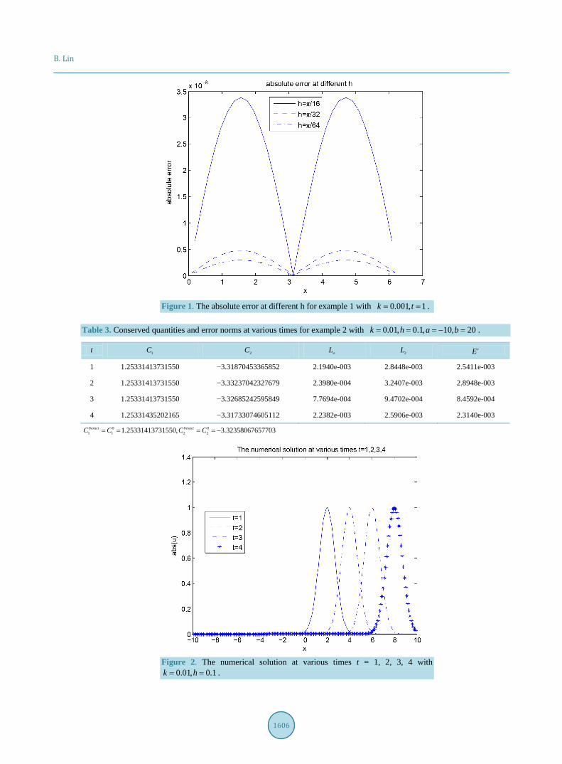
Figure 1. The absolute error at different h for example 1 with 0.001, 1k t= = .

Table 3. Conserved quantities and error norms at various times for example 2 with 0.01, 0.1, 10, 20k h a b= = = − = .

t 1C 2C L∞ 2L rE

1 1.25331413731550 −3.31870453365852 2.1940e-003 2.8448e-003 2.5411e-003

2 1.25331413731550 −3.33237042327679 2.3980e-004 3.2407e-003 2.8948e-003

3 1.25331413731550 −3.32685242595849 7.7694e-004 9.4702e-004 8.4592e-004

4 1.25331435202165 −3.31733074605112 2.2382e-003 2.5906e-003 2.3140e-003 0 0 0 0

1 1 2 21.25331413731550, 3.32358067657703exact exactC C C C= = = = −

Figure 2. The numerical solution at various times t = 1, 2, 3, 4 with

0.01, 0.1k h= = .

B. Lin

1607

Figure 3. The numerical solutions and analytical solutions for k = 0.01, h = 0.1 at time t = 3.

Figure 4 The numerical solutions and analytical solutions for k = 0.01, h = 0.1 at time t = 4.

Conserved quantities and error norms at various times are presented in Table 3. The numerical results reveal

that the values of 1C is almost constant while the values of 2C differ slightly and the errors are very small. The numerical solutions at various times are given in Figure 2. The numerical solutions and analytical solu-

tions at time 3t = and 4t = are shown in Figure 3 and Figure 4, respectively. The absolute error at time 3t = and 4t = are plotted in Figure 5 and Figure 6, respectively. It observed that (1) the propagation of so-

litary wave is rightward while preserving unchanged shape; (2) our method gives a good approximation com-pared with the exact solutions.

6. Conclusion A numerical method based on exponential spline interpolation function is applied to study a class of nonlinear Schrödinger equation. We use exponential spline collocation method, which results in tri-diagonal systems of

B. Lin

1608

Figure 5. The absolute error for k = 0.01, h = 0.1 at time t = 3.

Figure 6. The absolute error for k = 0.01, h = 0.1 at time t = 4.

equations that can be solved efficiently by the Thomas algorithm. The numerical simulations confirm and dem-onstrate the reliability and efficiency of the schemes and tell us that the method is applicable technique, rela-tively simple and approximates the exact solution very well.

Acknowledgements The authors would like to thank the editor and the reviewers for their valuable comments. This work was sup-ported by the Natural Science Foundation of Guangdong (2015A030313827).

References [1] Infeld, E. (1984) Nonlinear Waves: From Hydrodynamics to Plasma Theory, Advances in Nonlinear Waves. Pitman,

Boston.

B. Lin

1609

[2] Nore, C., Abid, A. and Brachet, M. (1996) Small-Scale Structures in Three-Dimensional Hydrodynamics and Magne-tohyrodynamic Turbulence. Springer, Berlin.

[3] Agrawal, G.P. (2001) Nonlinear Fibei Optics. 3rd Edition, Academic Press, San Diego. [4] Fordy, A.P. (1990) Soliton Theory: A Survey of Results. Manchester University Press, Manchester. [5] Bruneau, C.H., Di Menza, L. and Lerhner, T. (1999) Numerical Resolution of Some Nonlinear Schrödinger-Like Equ-

ation in Plasmas. Numerical Methods for Partial Differential Equations, 15, 672-696. http://dx.doi.org/10.1002/(SICI)1098-2426(199911)15:6<672::AID-NUM5>3.0.CO;2-J

[6] Bang, O., Christiansen, P.L., Rasmussen, K. and Gaididei, Y.B. (1995) The Role of Nonlinearity in Modeling Energy Transfer in Schibe Aggregates. In: Nonlinear Excitations in Biomolecules, Springer, Berlin, 317-336. http://dx.doi.org/10.1007/978-3-662-08994-1_24

[7] Ferreira, M.F., Faco, M.V., Latas, S.V. and Sousa, M.H. (2005) Optical Solitons in Fibers for Communication Systems. Fiber and Integrated Optics, 24, 287-313. http://dx.doi.org/10.1080/01468030590923019

[8] Zhang, J.F., Dai, C.Q., Yang, Q. and Zhu, J.M. (2005) Variable-Coefficient F-Expansion Method and Its Application to Nonlinear Schrödinger Equation. Optics Communications, 252, 408-421. http://dx.doi.org/10.1016/j.optcom.2005.04.043

[9] Zhang, J.L., Li, B.A. and Wang, M.L. (2009) Soliton Propagation in a System with Variable Coefficients. Chaos Soli-tons Fractals, 39, 858-865. http://dx.doi.org/10.1016/j.chaos.2007.01.116

[10] Taha, T.R. and Ablowitz, M.J. (1984) Analytical and Numerical Aspects of Certain Nonlinear Evolution Equations. II. Numerical, Nonlinear Schrödinger Equation. Journal of Computational Physics, 55, 203-230. http://dx.doi.org/10.1016/0021-9991(84)90003-2

[11] Zhang, L. (2005) A High Accurate and Conservative Finite Difference Scheme for Nonlinear Schrödinger Equation. Acta Mathematicae Applicatae Sinica, 28, 178-186.

[12] Duan, A. and Rong, F. (2013) A Numerical Scheme for Nonlinear Schrödinger Equation by MQ Quasi-Interpolatin. Engineering Analysis with Boundary Elements, 37, 89-94. http://dx.doi.org/10.1016/j.enganabound.2012.08.006

[13] Dag, I. (1999) A Quadratic B-Spline Finite Element Method for Solving Nonlinear Schrödinger Equation. Computer Methods in Applied Mechanics and Engineering, 174, 247-258. http://dx.doi.org/10.1016/S0045-7825(98)00257-6

[14] Dehghan, M. and Taleei, A. (2010) A Compact Split-Step Finite Difference Method for Solving the Nonlinear Schrödinger Equations with Constant and Variable Coefficients. Computer Physics Communications, 181, 43-51. http://dx.doi.org/10.1016/j.cpc.2009.08.015

[15] Dehghan, M. and Taleei, A. (2011) A Chebyshev Pseudospectral Multidomain Method for the Soliton Solution of Coupled Nonlinear Schrödinger Equations. Computer Physics Communications, 182, 2519-2529. http://dx.doi.org/10.1016/j.cpc.2011.07.009

[16] Mohammadi, R. (2014) An Exponential Spline Solution of Nonlinear Schrödinger Equations with Constant and Varia-ble Coefficients. Computer Physics Communications, 185, 917-932. http://dx.doi.org/10.1016/j.cpc.2013.12.015

[17] Lin, B. (2013) Parametric Cubic Spline Method for the Solution of the Nonlinear Schrödinger Equation. Computer Physics Communications, 184, 60-65. http://dx.doi.org/10.1016/j.cpc.2012.08.010

[18] Lin, B. (2015) Septic Spline Function Method for the Solution of the Nonlinear Schrödinger Equation. Applicable Analysis, 94, 279-293. http://dx.doi.org/10.1080/00036811.2014.890709

[19] Wang, S.S. and Zhang, L. (2011) Split-Step Orthogonal Spline Collocation Methods for Nonlinear Schrödinger Equa-tions in One, Two, and Three Dimensions. Applied Mathematics and Computation, 218, 1903-1916. http://dx.doi.org/10.1016/j.amc.2011.07.002

[20] Mohebbi, A. and Dehghan, M. (2009) The Use of Compact Boundary Value Method for the Solution of Two-Dimensional Schrödinger Equation. Journal of Computational and Applied Mathematics, 225, 124-134. http://dx.doi.org/10.1016/j.cam.2008.07.008

[21] Ismail, M.S. and Taha, T.R. (2007) A Linearly Implicit Conservative Scheme for the Coupled Nonlinear Schrodinger Equation. Mathematics and Computers in Simulation, 74, 302-311. http://dx.doi.org/10.1016/j.matcom.2006.10.020

Submit or recommend next manuscript to SCIRP and we will provide best service for you: Accepting pre-submission inquiries through Email, Facebook, LinkedIn, Twitter, etc. A wide selection of journals (inclusive of 9 subjects, more than 200 journals) Providing 24-hour high-quality service User-friendly online submission system Fair and swift peer-review system Efficient typesetting and proofreading procedure Display of the result of downloads and visits, as well as the number of cited articles Maximum dissemination of your research work

Submit your manuscript at: http://papersubmission.scirp.org/