spline orbifolds - graz university of · pdf filespline orbifolds johannes wallner, ... we de...

Spline Orbifolds

Johannes Wallner, Helmut Pottmann

Abstract. In order to obtain a global principle for modeling closedsurfaces of arbitrary genus, first hyperbolic geometry and then discretegroups of motions in planar geometries of constant curvature are studied.The representation of a closed surface as an orbifold leads to a naturalparametrization of the surfaces as a subset of one of the classical geome-tries S

2, E2 and H

2. This well known connection can be exploited todefine spline function spaces on abstract closed surfaces and use theme. g. for approximation and interpolation problems.

§1. Geometries of Constant Curvature

We are going to define three geometries consisting of a set of points, a setof lines, and a group of congruence transformations: The geometry of theeuclidean plane E2, the geometry of the unit sphere S2 of euclidean E3, andthe geometry of the hyperbolic plane H2. The geometries of E2 and S2 arewell known: the hyperbolic plane will be presented in the next subsections.For more details, see for instance (Alekseevskij et al., 1988).

It is possible to define hyperbolic geometry in a completely synthetic way.We could use a system of axioms for euclidean geometry and then negate theparallel postulate or one of its equivalents. Any structure satisfying the axiomswould be called a model of hyperbolic geometry. We would have to verify thatall models, including the classical ones, the Poincare and the Klein model, areisomorphic. We start from a different point of view: We first define a set ofpoints, lines and congruence transformations, as linear as possible, and thenshow some structures isomorphic to it. The reader then will see the differenceto euclidean or spherical geometry.

Curves and Surfaces with Applications in CAGD 445A. Le Mehaute, C. Rabut, and L. L. Schumaker (eds.), pp. 445–464.

Copyright oc 1997 by Vanderbilt University Press, Nashville, TN.

ISBN 0-8265-1293-3.

All rights of reproduction in any form reserved.

446 J. Wallner, H. Pottmann

��

��

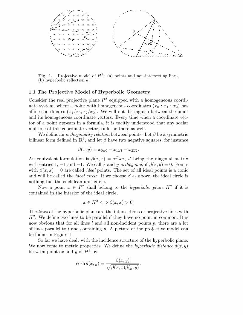
Fig. 1. Projective model of H2: (a) points and non-intersecting lines,

(b) hyperbolic reflection κ.

1.1 The Projective Model of Hyperbolic Geometry

Consider the real projective plane P 2 equipped with a homogeneous coordi-nate system, where a point with homogeneous coordinates (x0 : x1 : x2) hasaffine coordinates (x1/x0, x2/x0). We will not distinguish between the pointand its homogeneous coordinate vectors. Every time when a coordinate vec-tor of a point appears in a formula, it is tacitly understood that any scalarmultiple of this coordinate vector could be there as well.

We define an orthogonality relation between points: Let β be a symmetricbilinear form defined in IR3, and let β have two negative squares, for instance

β(x, y) = x0y0 − x1y1 − x2y2.

An equivalent formulation is β(x, x) = xT Jx, J being the diagonal matrixwith entries 1, −1 and −1. We call x and y orthogonal, if β(x, y) = 0. Pointswith β(x, x) = 0 are called ideal points. The set of all ideal points is a conicand will be called the ideal circle. If we choose β as above, the ideal circle isnothing but the euclidean unit circle.

Now a point x ∈ P 2 shall belong to the hyperbolic plane H2 if it iscontained in the interior of the ideal circle,

x ∈ H2 ⇐⇒ β(x, x) > 0.

The lines of the hyperbolic plane are the intersections of projective lines withH2. We define two lines to be parallel if they have no point in common. It isnow obvious that for all lines l and all non-incident points p, there are a lotof lines parallel to l and containing p. A picture of the projective model canbe found in Figure 1.

So far we have dealt with the incidence structure of the hyperbolic plane.We now come to metric properties. We define the hyperbolic distance d(x, y)between points x and y of H2 by

coshd(x, y) =|β(x, y)|√

β(x, x)β(y, y).

Spline Orbifolds 447

We leave the verification of the fact that always β(x, x)β(y, y) ≤ β(x, y)2 tothe reader. This metric satisfies the triangle inequality and is compatible withthe definition of lines, in the sense that they are precisely the geodesic curveswith respect to this metric.

Hyperbolic congruence transformations will be those projectivetransformations, which map H2 onto H2 and preserve hyperbolic distances.For this reason and also because it is shorter, we will call them isometries ormotions. We express the isometric property in matrix form: for each projec-tive transformation κ there is a matrix such that in homogeneous coordinates

κ(x) = A · x.

It is easy to see that the condition d(x, y) = d(κ(x), κ(y)) for all x ∈ H2 isequivalent to

AT JA = λJ with λ > 0,

and that there are the following types of hyperbolic isometries:

1) the identity transformation;

2) hyperbolic reflections, which leave the points on a hyperbolic line fixedand reverse orientation (see Figure 1b);

4) hyperbolic translations, which preserve orientation and leave nopoint of H2 fixed, but a hyperbolic line is mapped onto itself;

5) hyperbolic rotations, which leave one point of H2 fixed and preserve ori-entation (for a picture in a different model, see Figure 3);

6) ideal hyperbolic transformations which leave no point of H2 fixed, and noline is mapped to itself, but orientation is preserved;

7) the remaining hyperbolic isometries reverse orientation and are the prod-uct of a hyperbolic reflection by one of the above.

The model of the hyperbolic plane just described is called the projective

or Klein model. In this model hyperbolic geometry appears as a subset ofprojective geometry: the point set is a subset of the projective point set, thelines are the appropriate subsets of projective lines, and hyperbolic isometriescan be expressed in matrix form.

What remains to be defined is the hyperbolic angle. We will do this in adifferent model, which will also explain the name “hyperbolic”.

1.2 The Hyperboloid Model of Hyperbolic Geometry

In IR3, β(x, x) = 0 is the equation of a quadratic cone with apex at the origin,and β(x, x) = 1 is the equation of a two-sheeted hyperboloid, which can beseen as the unit sphere with respect to the pseudo-euclidean scalar productβ. We call the “upper sheet” of this unit sphere the hyperbolic plane:

x ∈ H2 ⇐⇒ β(x, x) = 1 and x0 > 0.

There is an obvious one-to-one correspondence between the hyperbolic planedefined in Section 1.1 and the hyperbolic plane defined in this subsection.


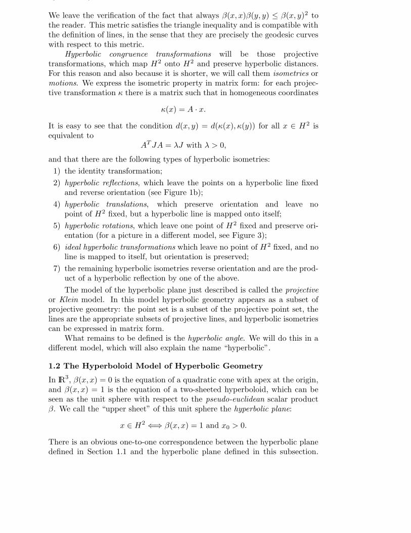
Fig. 2. The hyperboloid model X ⊂ IR3 of H2 and the correspondence

between hyperboloid and projective model, which appears as a unit disktangent to X.

Given a projective point, its uniquely defined coordinate vector x withβ(x, x) = 1 and x0 > 0 defines the corresponding point of the hyperboloidmodel. It is easy to transfer lines and hyperbolic isometries to the hyperboloidmodel: Hyperbolic lines have linear equations and therefore are intersectionsof H2 with two-dimensional linear subspaces of IR3. A picture of the hyper-boloid model is given in Figure 2.

In the projective model, a hyperbolic isometry given by its matrix A isequivalently described by any scalar multiple of A. Now scale A such that

AT JA = J.

Then the unit hyperboloid β(x, x) = 1 is invariant under multiplication byA. Conversely, as scalar products can be expressed in terms of distances,the invariance of the unit hyperboloid implies AT JA = J . If A interchangesthe two sheets of the unit hyperboloid, multiply A by −1. Thus, withoutloss of generality, we call all linear automorphisms of IR3 which map H2 ontoitself hyperbolic isometries and this definition is compatible with the definitiongiven in Section 1.1.

A scalar product β always defines an angle between vectors x and y: InIR3 the pseudo-euclidean angle 6 (x, y) is partially defined by

λ =β(x, y)√

β(x, x)β(y, y)if β(x, x)β(y, y) > 0

cos 6 (x, y) = λ if |λ| ≤ 1

cosh 6 (x, y) = |λ| if |λ| ≥ 1


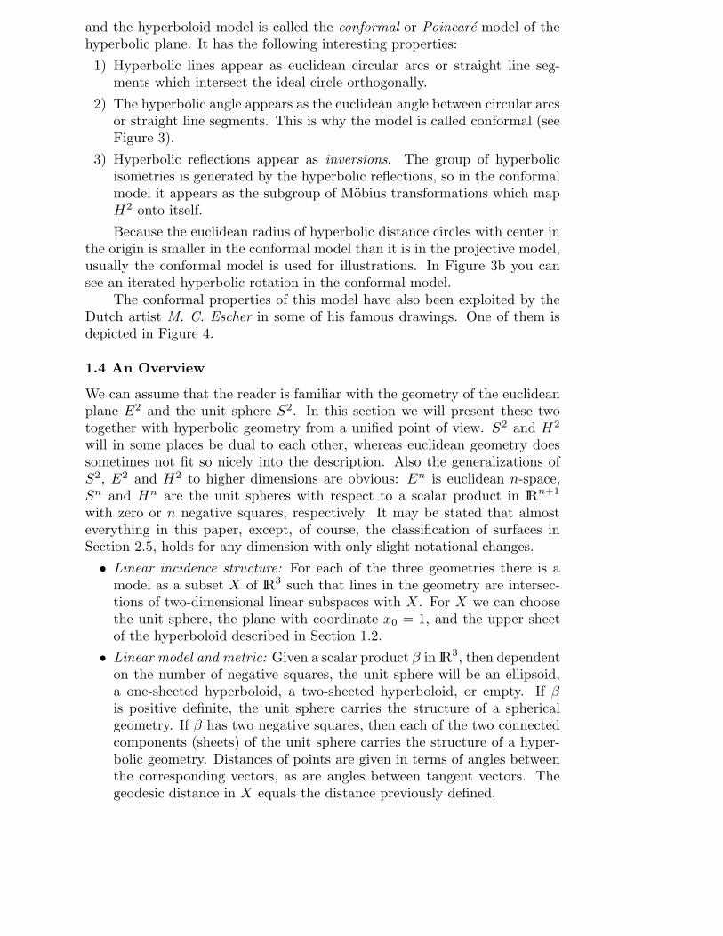
Fig. 3. Conformal model: hyperbolic rotation.

In every case where we will calculate an angle it has to be verified that β(x, x)·β(y, y) > 0. In most cases we leave this verification to the reader. It isclear that the pseudo-euclidean angle of vectors x and y corresponds to thehyperbolic distance defined in Section 1.1. The hyperbolic angle between linesmeeting in x is defined as the pseudo-euclidean angle of tangent vectors at x.Because all vectors v tangent to H2 in a point x satisfy β(v, v) < 0, the anglebetween them is defined.

We define the geodesic distance between points x and y on a smoothsurface X in IRn as the infimum of the arc-lengths of smooth curves c joiningx and y in X. Arc-lengths are measured by means of the scalar product β:We can define the norm of a vector by ‖x‖2 = |β(x, x)| and measure the arclength by

∫‖c(t)‖dt. It is easy to see that for H2 we can explicitly find the

curves for which the infimum, actually then the minimum, is attained: Thegeodesic distance is the arc-length of the unique hyperbolic line joining x andy and equals the hyperbolic distance d(x, y).

1.3 The Conformal Model of Hyperbolic Geometry

Distorting the projective model leads to a new model of hyperbolic geometrywith some other special metric properties: Let H2 be the interior of the unitcircle and define σ : H2 → H2 in affine coordinates by

(x, y) 7→1

1 −√

1 − x2 − y2(x, y).

Thus points will be moved a bit towards the origin. Hyperbolic lines willbe σ-images of hyperbolic lines defined in Section 1.1. If κ is a hyperbolicisometry as defined in Section 1.1, then σκσ−1 shall be a congruence trans-formation. This geometry which is obviously isomorphic to the projective


and the hyperboloid model is called the conformal or Poincare model of thehyperbolic plane. It has the following interesting properties:

1) Hyperbolic lines appear as euclidean circular arcs or straight line seg-ments which intersect the ideal circle orthogonally.

2) The hyperbolic angle appears as the euclidean angle between circular arcsor straight line segments. This is why the model is called conformal (seeFigure 3).

3) Hyperbolic reflections appear as inversions. The group of hyperbolicisometries is generated by the hyperbolic reflections, so in the conformalmodel it appears as the subgroup of Mobius transformations which mapH2 onto itself.

Because the euclidean radius of hyperbolic distance circles with center inthe origin is smaller in the conformal model than it is in the projective model,usually the conformal model is used for illustrations. In Figure 3b you cansee an iterated hyperbolic rotation in the conformal model.

The conformal properties of this model have also been exploited by theDutch artist M. C. Escher in some of his famous drawings. One of them isdepicted in Figure 4.

1.4 An Overview

We can assume that the reader is familiar with the geometry of the euclideanplane E2 and the unit sphere S2. In this section we will present these twotogether with hyperbolic geometry from a unified point of view. S2 and H2

will in some places be dual to each other, whereas euclidean geometry doessometimes not fit so nicely into the description. Also the generalizations ofS2, E2 and H2 to higher dimensions are obvious: En is euclidean n-space,Sn and Hn are the unit spheres with respect to a scalar product in IRn+1

with zero or n negative squares, respectively. It may be stated that almosteverything in this paper, except, of course, the classification of surfaces inSection 2.5, holds for any dimension with only slight notational changes.

• Linear incidence structure: For each of the three geometries there is amodel as a subset X of IR3 such that lines in the geometry are intersec-tions of two-dimensional linear subspaces with X. For X we can choosethe unit sphere, the plane with coordinate x0 = 1, and the upper sheetof the hyperboloid described in Section 1.2.

• Linear model and metric: Given a scalar product β in IR3, then dependenton the number of negative squares, the unit sphere will be an ellipsoid,a one-sheeted hyperboloid, a two-sheeted hyperboloid, or empty. If βis positive definite, the unit sphere carries the structure of a sphericalgeometry. If β has two negative squares, then each of the two connectedcomponents (sheets) of the unit sphere carries the structure of a hyper-bolic geometry. Distances of points are given in terms of angles betweenthe corresponding vectors, as are angles between tangent vectors. Thegeodesic distance in X equals the distance previously defined.


Fig. 4. M. C. Escher’s ”Circle Limit IV”, (c) 1997 Cordon Art – Baarn– Holland. All rights reserved.

• Congruence transformations: In the linear models X ⊂ IR3 of S2 andH2, the group of motions or isometries consists of the restrictions L|X ofthose linear automorphisms L of IR3 which map X onto itself.

• Curvature: The sphere, the euclidean plane and the hyperbolic planeare Riemannian manifolds of constant Gaussian curvature, the value ofwhich is 1, 0 and −1, respectively. From the Gauss-Bonnet theorem itthen follows that the angle sum in a triangle is greater than, equal to, orless than π, respectively. Moreover, the absolute value of the differenceis the area of the triangle as of a Riemannian manifold.

§2. Discrete Motion Groups and Orbifolds

In this section we define the factor orbifold X/H where X is one of E2, S2

or H2, and H is a discrete transformation group acting on X. X will alwaysdenote one of the three geometries, and its motion group will be denoted by


��

� ��

��

��

� ��

��

� � ��

��

��

Fig. 5. The torus as an orbifold.

G. We will not be able to present a complete theory, and we simplify somenotions in some places.

For a detailed presentation, see for instance (Ratcliffe, 1994), (Vinbergand Shvartsman, 1988) or (Zieschang et al., 1980). For a well illustrated bookwhich is easy to read, see for instance (Week, 1985).

2.1 Discrete Transformation Groups

We will consider groups H of motions acting on X, which means that eachh ∈ H is an isometry h : X → X and h1(h2(x)) = (h1 · h2)(x). The identitytransformation will always be denoted by e. We write h(x) for the h-image ofan x ∈ X and h(K) for the h-image of a subset K ⊂ X. We call a group Hacting on X discrete if for every compact set K the intersection K ∩ h(K) isnonempty only for finitely many h ∈ H. This implies that the orbit {h(x), h ∈H} of a point x is discrete, i. e., it has no accumulation point. An example forthis is the group H = ZZ2 acting as a group of translations on the euclideanplane: The pair (i, j) of integers acts on X = E2 by (x, y) 7→ (x + i, y + j). Itis only a change in notation if we consider H as a subgroup of the euclideanmotion group. A picture can be seen in Figure 5.

For a group H acting on X, the stabilizer Hx of x is the subgroup of allthose h ∈ H with h(x) = x. If H is discrete, obviously Hx is finite. Theorder of x is the cardinality of its stabilizer. In the example given above allstabilizers are trivial. We call such actions free.

If x and y are not antipodal points of the sphere, the unique shortestsegment joining them is called their convex hull, and a set C is called convex,if for all x, y ∈ C the convex hull of x and y is in C. Then a convex polygon

is defined as the convex hull of a finite non-collinear set of points. Edges andvertices are defined in the obvious way. Note that a convex polygon is alwaysthe closure of its interior.

2.2 Fundamental Domains

A fundamental domain F of a discrete motion group H is a set which isthe closure of its interior and fulfills the following conditions: 1) the sets


h(F ), h ∈ H cover X, and 2) if h1(F ) and h2(F ) have an interior point incommon, then h1 = h2. There are discrete groups of motions which have noconvex polygons as fundamental domains, for instance the discrete group oftranslations along integer multiples of one fixed vector in E2. We will nottry to generalize the notion of polygon such that it covers all discrete motiongroups (which is possible), but we restrict ourselves to groups which possessconvex fundamental polygons.

We denote the edges of the fundamental polygon F by s0, . . . , sn−1, sn =s0. The intersection of edges si ∩ si+1 is a vertex vi. By subdividing finitelymany edges and introducing new vertices it is possible to achieve that the in-tersection of F with any h(F ) is either empty or an edge. We call the uniquelydefined motion h ∈ H for which F ∩ h(F ) = si the adjacency transformation

of the edge sj . We call a sequence h1(F ), . . . , hn(F ) a chain of polygons, ifthe intersection hi(F ) ∩ hi+1(F ) is an edge. Because any two h ∈ H can beconnected by a chain, the group H is entirely generated by the finitely manyadjacency transformations of one fundamental polygon.

If an adjacency transformation maps si to sj , then we write si = s′j .Obviously then the inverse adjacency transformation maps sj to si, so s′i = sj .For the example given above, the adjacency transformations are indicated inFigure 5.

2.3 Defining Relations

We write hs for the adjacency transformation with F ∩hs(F ) = s. A sequencehs1

, . . . , hsnof adjacency transformations with hs1

· . . . · hsn= e corresponds

to a chain F0 = F, F1 = hs1(F ), F2 = hs1

(hs2(F )), . . . , Fn = F0 of polygons.

Such a chain is called a cycle.Let s, s′ be edges with hs(s

′) = s and hs′(s) = s′. Then obviouslyhshs′ = e and F, hs(F ), hshs′(F ) = F is a cycle. Formally, we write

ss′ = e.

Also for all vertices v there is a cycle of polygons consisting of all polygonscontaining v in the order in which they are encountered when cycling v. Thecorresponding sequence hs1

, . . . , hsnof adjacency transformations gives the

formal relations1s2 . . . sn = e,

which is called a Poincare relation. The importance of the Poincare relationsis shown by the following

Theorem. Let H be a group with a convex fundamental polygon. Denote

its set of edges by S and the set of relations ss′ = e together with all Poincare

relations with R. Then the abstract group with generator set S and relations

R is isomorphic to H.

In the example given above, all adjacency transformations are trans-lations. They correspond to the edges s0, s1, s2, s3 and s′0 = s2, s′1 = s3


(see Figure 5). The four Poincare relations are s0s1s2s3 = e, s1s2s3s0 = e,s2s3s0s1 = e and s3s0s1s2 = e. Obviously s2s0 = e and s1s3 = e. So we caneliminate s2 and s3. Each Poincare relation implies the other three. It followsthat H as an abstract group is isomorphic to the group with generators s0, s1

and the single relation s0s1s−10 s−1

1 = e, or, equivalently, s0s1 = s1s0. Thismeans that H is a free abelian group with free generators s0 and s1.

A natural question to ask now is: Given a convex polygon F and foreach edge s an adjacency transformation hs, such that (a) F ∩ hs(F ) = s,(b) hs(s

′) = s implies hs′(s) = s′, and (c) hshs′ = e. Suppose further that(d) for each vertex v of F there are adjacency transformations hs1

, . . . hsn

such that their product equals e and the polygons hs1hs2

. . . hsi(F ) form a

“circuit” around v. Does there exist a discrete group of motions having F asfundamental polygon and hs as adjacency transformations? The answer, dueto Poincare, is yes.

2.4 Orbifolds

Let H be a discrete group of motions in one of the three geometries E2, S2 orH2. By identifying all points h(x), h ∈ H, we get the points of the orbifold

X/H. This definition, however, gives only the orbifold as a set, without addi-tional structures. They are to be defined by means of the canonical projection

p : X → X/H which maps an x ∈ X to its orbit. The topology on X/H isdefined as the final topology of p: U is open if and only if p−1(U) is open.The incidence structure is directly mapped by p: A line segment in X/H isthe p-image of a line segment of X. The distance between x, y in X/H is theminimum of distances of points in p−1(x) and p−1(y) measured in X.

An example for an orbifold which is very well known, but, in some senseis not typical, is the torus. It appears as the orbifold X/H if X = E2 andH is the discrete group of translations along integer multiples of two basisvectors e1 and e2 (see Figure 5). The order of all points x equals 1, and sofor all y in p−1(x) there is a neighborhood of y which is mapped isometrically(and, of course, homeomorphically) to X/H. This need not be the case, andhappens if and only if some h ∈ H has a fixed point. These orbifolds havemetric singularities and could also be used for modeling surfaces, but we willomit them in order to keep the presentation simple.

2.5 Surfaces

Our aim is to find discrete groups H in a geometry X of constant curvaturesuch that the corresponding orbifold X/H is a compact surface, orientable ornonorientable, of arbitrary genus g. It is well known that the compact surfaceswithout boundary are precisely the spheres with g handles and the sphereswith g crosscaps. For the classification of surfaces from the topological, dif-ferentiable, or combinatorial viewpoint, see textbooks of algebraic topology,differential topology or combinatorial topology, for instance (Hirsch, 1976) or(Kinsey, 1993).


!#"

!%$ "

!'&

!%$&(

Fig. 8. Klein bottle.

It is well known that the following discrete transformation groups H invarious geometries X lead to all compact surfaces:

• The sphere: S2 itself as the orientable surface of genus 0 is one of theprimitive geometries. Formally, let X = S2 and H = {e}.

• The projective plane: P 2 is obtained by identifying antipodal points inS2. If s denotes the antipodal map, then P 2 = S2/H with H = {e, s}.A fundamental polygon is the upper hemisphere.

• The torus: Letting X = E2 and H equal the group generated by thetranslations along two linearly independent vectors gives the torus, whichis the orientable surface of genus 1. A fundamental polygon is the paral-lelogram spanned by a lattice basis.

• The Klein bottle: Letting X = E2 and H equal the group generatedby the adjacency transformations depicted in Figure 8 gives the nonori-entable surface of genus 2, which is called the Klein bottle.

• Orientable surfaces of higher genus: In the conformal model of the hyper-bolic plane, consider the points (r cos(2kπ/l), r sin(2kπ/l)) with l = 4g,g ≥ 2 and k = 0, . . . , l− 1. The convex hull F of these points is a regular4g-gon, with interior hyperbolic angles α depending on the value of r (seeFigure 9). It is easily seen that α tends to 0 as r tends to 1, and α tendsto π − 2π/l as r tends to 0. By continuity, for all l there is a value of rsuch that the interior angle α equals 2π/l. Now denote the edges of F bya1, b1, a

′1, b

′1, . . . , ag, bg, a

′g, b

′g and define orientation-preserving adjacency

transformations which map ak to a′k, bk to b′k and vice versa, for all k.

Then the Poincare relations will be equivalent to the relation

a1b1a′1b

′1a2b2a

′2b

′2 . . . agbga

′gb

′g = e.


)+*

, *

)�- *

, - *)/.

, .

)�-.

, - .

021�3

0#4 3

0 465

0'1 5

)%*

)�- *

) .

) - .)�7

)�-7

)�8

) -8

021 3

0 1 50 1:9

021<;

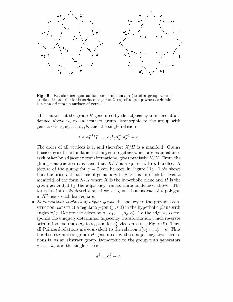
Fig. 9. Regular octogon as fundamental domain (a) of a group whoseorbifold is an orientable surface of genus 2 (b) of a group whose orbifoldis a non-orientable surface of genus 4.

This shows that the group H generated by the adjacency transformationsdefined above is, as an abstract group, isomorphic to the group withgenerators a1, b1, . . . , ag, bg and the single relation

a1b1a−11 b−1

1 . . . agbga−1g b−1

g = e.

The order of all vertices is 1, and therefore X/H is a manifold. Gluingthose edges of the fundamental polygon together which are mapped ontoeach other by adjacency transformations, gives precisely X/H. From thegluing construction it is clear that X/H is a sphere with g handles. Apicture of the gluing for g = 2 can be seen in Figure 11a. This showsthat the orientable surface of genus g with g > 1 is an orbifold, even amanifold, of the form X/H where X is the hyperbolic plane and H is thegroup generated by the adjacency transformations defined above. Thetorus fits into this description, if we set g = 1 but instead of a polygonin H2 use a euclidean square.

• Nonorientable surfaces of higher genus: In analogy to the previous con-struction, construct a regular 2g-gon (g ≥ 3) in the hyperbolic plane withangles π/g. Denote the edges by a1, a

′1, . . . , ag, a

′g. To the edge ak corre-

sponds the uniquely determined adjacency transformation which reversesorientation and maps ak to a′

k, and for a′k vice versa (see Figure 9). Then

all Poincare relations are equivalent to the relation a21a

22 . . . a2

g = e. Thusthe discrete motion group H generated by these adjacency transforma-tions is, as an abstract group, isomorphic to the group with generatorsa1, . . . , ag and the single relation

a21 . . . a2

g = e.


The order of all vertices equals 1, and therefore X/H is a manifold. Itis nonorientable because H contains orientation reversing motions. Fromthe gluing construction it is clear that X/H is a sphere with g crosscaps.

The Klein bottle (g = 2) and the projective plane (g = 1) fit into thisformalism, if we choose a euclidean square or a spherical 2-gon (such asthe northern hemisphere) instead.

§3. Functions on Surfaces

3.1 Group-Invariant Functions

We call a function f : X → R invariant with respect to the group H, if

f(h(x)) = f(x) for all x ∈ X,h ∈ H.

If p : X → X/H denotes the canonical projection, an H-invariant functiondirectly leads to a function f whose domain is the factor orbifold:

f : X/H → R, f(p(x)) = f(x)

and vice versa: a function f defined on X/H gives rise to an H-invariantfunction

f : X → R, f(x) = f ◦ p(x).

If the range R is the real number field IR and f is a function defined on X,then we can build an H-invariant function g from f by letting

g(x) =∑

h∈H

f(h(x)).

Of course it has to be verified that this sum makes sense. If X is the sphere,every discrete motion group is finite, and the sum above is finite. So everyproperty of f which is invariant with respect to finite sums is preserved, sofor instance continuity or differentiability.

If f has compact support, then for all x there is a neighborhood U of xsuch that the sum defined above is finite in U , by discreteness of H. So alllocal properties which are invariant with respect to finite sums are preserved,for instance continuity or differentiability.

If X/H is a manifold, it is clear that f : X/H → IR is continuous (differ-

entiable, of class Cr, of class C∞) if and only if the corresponding f : X → IRhas this property. If X/H is an orbifold with metric singularities, we avoiddifficulties by defining that an f defined on X/H is differentiable (of class Cr,of class C∞) if the corresponding f has this property.

The above sum can make sense even if f does not have compact support.It is sufficient that f decreases fast enough. An example for a summablefunction whose sum is of class C∞ is the Gaussian f(x) = exp(−d(x,m)2) in

E2 and H2 (note that in S2 f is not differentiable everywhere).


3.2 Polynomial and Rational Functions

For each of the three geometries S2, E2 and H2 we have found a model as asubset X of IR3. This enables us to define polynomial or rational functionson X as the restriction of polynomial or rational functions defined in IR2 toX. It is well known that both S2 and H2 possess rational parametrizationswhich can be given by stereographic projections: The mapping σ defined by

σ : IR2 → S2 \ {(−1, 0, 0)}, (p, q) 7→1

1 + p2 + q2(1 − p2 − q2, 2p, 2q)

is one-to-one. Also, the mapping σ defined by

σ : D → H2, (p, q) 7→1

1 − p2 − q2(1 + p2 + q2, 2p, 2q)

with D being the interior of the unit circle, is one-to-one. If f is a polynomialdefined in IR3, then f ◦ σ is a rational function defined in the domain of σ.

We want to indicate how modeling of closed surfaces with the aid ofpiecewise rational functions is possible. First we give an easy example whichshows how to proceed in the not so trivial cases: The B-spline basis functionson the real line are well known, and so are tensor product B-splines in E2.We define a knot sequence on the x1-axis which is periodic and has period 1.This means that if t is a knot, then t + k is a knot for every integer k. Thesame we do for the x2-axis, and then we consider the B-spline basis functionsBi(x1) and Bj(x2) which correspond to this knot sequences. Their productsBij(x1, x2) defined in the plane form a partition of unity. There are finitelymany functions Bij(x1, x2) such that all others can be expressed in the formB(x1, x2) = Bij(h(x1, x2)) where h is an element of the translation group Hgenerated by translations along the unit vectors in x1- and x2-direction. AllBij ’s are compactly supported, so the functions

Cij(x) =∑

h∈H

Bij(h(x))

are well defined, are group-invariant, and form a partition of unity. Thusthere are finitely many functions Cij defined on the torus E2/H such that

Cij(p(x)) = Cij(x) and∑

Cij(p(x)) = 1 for all x ∈ E2,

where p is the canonical projection which maps a point x = (x1, x2) to itsorbit.

The preceding paragraph contained nothing new. It could be said that itis a complicated formulation of the simple fact that “closing” B-spline curvesis also possible in the plane, and analogously to closed curves which can beviewed as defined on the circle, this closing operation yields a closed surfacedefined on the torus. On other surfaces the process of making a functiongroup-invariant may be more complicated, but the principle is the same andhas been shown in Section 3.1.


3.3 Simplex Splines and a DMS-Spline Space

It is well known that the restriction of homogeneous B-splines to the sphereleads to spline spaces of functions whose domain are subsets of the surface ofthe sphere, see e. g. (Alfeld et al., 1996). We want to show that the conceptof simplex spline is not restricted to the sphere and that there is a naturalgeneralization to abstract surfaces of higher genus.

Choose a basis b1, . . . , bn ∈ IRn. Then for all v ∈ IRn there is a uniquelinear combination v1b1+· · ·+vnbn equal to v. For all n-tuples k = (k1, . . . , kn)of integers we define the function

Bk : IRn → IR, v 7→(k1 + . . . + kn)!

k1! . . . kn!vk1

1 . . . vkn

n ,

which is called a homogeneous Bernstein basis polynomial of degree

|k| = k1 + · · · + kn. Any linear combination of homogeneous Bernstein basispolynomials of the same degree is called a homogeneous Bernstein polyno-

mial. For such a polynomial p =∑

|k|=d ckBk the equation p(λv) = λdp(v)

holds. If X is the linear model of one of the three geometries S2, E2 orH2, the restrictions p|X are called spherical, planar or pseudo-spherical Bern-stein polynomials. Note that the planar Bernstein polynomials are just thewell-known triangular Bernstein polynomials in the plane.

Also the notion of simplex spline has a natural meaning in the linearmodel of S2, E2 and H2. We recall that the homogeneous simplex splineMB : IRn → IR is well defined for a set B = {b1, . . . , bm} of vectors as follows:

MB(v) = χB(v)/det(b1, . . . , bn)

MB(v) =∑

b∈T

λbMB\b(v)

if |B| = n

if |B| > n and v =∑

b∈T

λbb.

Here χB(v) equals 1 if all coordinates λi with respect to the basis B arepositive and zero if at least one is negative. T denotes an arbitrary n-elementsubset of B which is a basis of IRn. This defines the simplex spline in IRn

except in some subspaces. Now extend the simplex spline continuously. Thisgives a Cm−n function. It is natural to define spherical, planar or pseudo-spherical simplex splines as the restriction MB |X of simplex splines MB .

This allows the definition of a spline space analogous to the DMS-splinespaces introduced in (Dahmen et al., 1992). This is of theoretical interest,because it shows the existence of a spline space consisting of piecewise rationalfunctions of arbitrary finite differentiability defined on a surface of genus g overan arbitrary triangulation. The planar and the spherical variant of the DMS-spline space have already been defined, for instance in (Pfeifle and Seidel,1994).

Simplex splines are most easily made group-invariant if they are definedover a group-invariant triangulation. Here group-invariant means that everymotion h ∈ H maps the triangulation onto itself. One possibility to construct


Fig. 10. Group-invariant tesselation.

such a triangulation is the following: Choose a set V of vertices in a funda-mental domain of the group H and consider the set V = {h(v), h ∈ H, v ∈ V }.Then apply an algorithm which finds the edges of a triangulation with ver-tex set V and is designed such that it uses only information which can beexpressed in terms of the geometry, for instance distance. Then a congru-ence transformation κ applied to V must result in edges which are just theκ-images of the previous ones. Now it is clear that if V is group-invariant, sois the whole triangulation. An example of a triangulation which is invariantwith respect to the group corresponding to the orientable surface of genus 2is shown in Figure 10.

A function defined by means of the triangulation and the geometry alonethen is group-invariant. This is especially true for all functions which are de-fined by means of one of the linear models X ⊂ IR3 and are linearly dependenton the coordinate vectors of the vertices. One example of this is given by thesimplex splines defined above.

3.4 Approximation, Interpolation, Visualization

These tools can be used for approximation and interpolation of functionsdefined on a compact surface and also for visualizing such surfaces. This hasbeen pointed out by Ferguson and Rockwood (1993). The spherical, euclideanor hyperbolic area dµ defines a measure in X. If we assume that the boundaryof the fundamental domain F has measure zero, dµ naturally defines a measuredµ on X/H and we can define the space L2(X/H) with the scalar product

(f, g) =

∫

X/H

fgdµ =

∫

F

f gdµ


Fig. 11. (a) Gluing the boundary of an octogon together yields a surfaceof genus 2, (b) C

∞-approximation of a polyhedron.

in the well known way. The resulting norm will be denoted by ‖f‖2. Onetypical problem now is the following: Given a finite set B = {b1, . . . , bn} ofbasis functions and a function f on X/H, we seek a linear combination of thebi such that

‖f −∑

λibi‖2 → min .

This is a classical least squares problem and can easily be solved: If the bi

are orthonormal, λi = (f, bi) is the solution. If not, apply the Gram-Schmidtorthogonalization process. For interpolation we for instance introduce thespace L2

∆(X/H) with the scalar product

(f, g)∆ =

∫

X/H

∆f∆gdµ,

where ∆ is the Laplace-Beltrami operator on X/H which is inherited from X.This allows us to find in the linear solution space of the interpolation problem∑

λibi(xj) = cj a solution of minimal energy. It is also possible to extendinterpolation schemes which have been successfully employed for sphere-likesurfaces to the linear models of the S2, E2 and H2, for instant the hybridpatch of (Liu and Schumaker).

Modeling and visualization of compact surfaces is possible in the followingway: A closed surface in IR3 can be seen as an embedding (or, at least, an


immersion) of an abstract closed surface X/H into IR3. For each abstractpoint p ∈ X/H three coordinate values x1(p), x2(p) and x3(p) are given. Thismeans that we have three real functions x1, x2 and x3 whose domain is X/H.Equivalently, we have three H-invariant functions xi whose domain is X. Theyhave the property that the (x1, x2, x3)-image of X/H is homeomorphic toX/H. Thus approximation, interpolation and modeling of surfaces is nothingbut approximation, interpolation and modeling of three separate coordinatefunctions.

Suppose we are given a polyhedron with vertices p1, . . . , pn and we seeka C∞ approximation to it. We describe our solution to this problem, which istypical for the sort of problems arising in this context. The algorithm is thefollowing:1) Cut the polyhedron along four closed curves passing through one fixed

base point, such that the resulting surface becomes simply connected.An example of such a cutting is shown in Figure 11a. The cuts are incorrespondence to the fundamental polygon which is shown in Figure 9a.

2) Find finitely many points q1, . . . , qn in the fundamental octogon corre-sponding to the appropriate group H with the following property: If weconstruct a group-invariant triangulation with vertices h(qi), i = 1, . . . , n,h ∈ H, then this triangulation, when factored to the orbifold, is combi-natorically equivalent to the triangulation of the polyhedron.

This triangulation need not necessarily consist of triangles, it can alsobe a tesselation with n-gons of different shape and different number ofvertices. The vertices do not necessarily have to lie inside the fundamentalpolygon. The cuts and the 8-gon are merely a guide where to put theqi. For instance the tesselation shown in Figure 10 after factoring iscombinatorically equivalent to the polyhedron shown in Figure 11 aftersubdividing each of the squares in four parts.

3) Optimize the triangulation/tesselation with respect to appropriate crite-ria. For instance we can try to optimize the shape of the faces of thetriangulation/tesselation. In our case, the faces of the polyhedron aresquares, so we want the faces of the tesselation be as square-like as pos-sible. Because not for all vertices the number of faces containing thisvertex equals four, we have to compromise.

4) Find a one-to-one correspondence between X/H and the polyhedron, or,equivalently, find a covering map from X to the polyhedron which iscompatible with the triangulation. In our case this is done easily bymapping the 4-gons of the tesselation to the squares of the polyhedronin the obvious way.

5) To each point of X we assign the three coordinate values x1, x2, x3 ofits corresponding point on the polyhedron. This defines three continuousH-invariant functions on X.

6) Approximate the xi by functions yi which are linear combinations of C∞

basis functions, for instance Gaussians.

7) Use the three functions y1, y2 and y3 as coordinate functions of a surface


in IR3 whose parameter domain is X/H or X depending on the level ofabstraction. This is how Figure 11b was made.

If the correspondence between the points q1, . . . , qn of X/H and the verticesp1, . . . , pn is established, interactive modeling of polyhedra of similar shapeis easy. We can construct the correspondence between X/H a further poly-hedron P of the same shape by finding a correspondence between the modelpolyhedron and P . This is especially trivial if P combinatorically is just arefinement of the model polyhedron. The approximation problem for P isthen just the problem of approximation of three new coordinate functions.

If the basis functions bi are already orthonormal, approximation can bedone very quickly. Moving the vertices of the polyhedron, which can now beseen as control points of the surface, influences the approximant surface. De-pending on the type of basis function, the influence will be local or global. AsGaussians decrease rapidly, and in addition can be multiplied by compactlysupported bump functions to become compactly supported without essentiallychanging their global shape, we have local control. For implementation pur-poses, the basis functions with compact support are very convenient, becausethe handling of infinite sums can be avoided completely.

Modeling of Cr surfaces with polynomial coordinate functions is possibleif we choose the bi as simplex splines or homogeneous DMS-splines. Thisgives an algorithm which makes it possible to model surfaces of arbitrarydifferentiability, of arbitrary genus, over an arbitrary triangulation, withoutany boundary and gluing conditions. A more detailed theory and furtherexamples of this can be found in (Wallner, 1996).

References

1. Alekseevskij D. V., E. B. Vinberg and A. S. Solodovnikov, Geometry ofspaces of constant curvature, in: Itogi Nauki i Tekhniki, SovremennyeProblemy Matematiki, Fundamentalnye Napravleniya, Vol. 29, VINITI,Moscow 1988; English translation in: Encyclopedia of Mathematical Sci-ences 29, Springer Verlag 1993.

2. Alfeld P., M. Neamtu and L. L. Schumaker, Bernstein-Bezier polynomialson spheres and sphere-like surfaces, Comput. Aided Geom. Design 13

(1996), 333–349.

3. Dahmen W., C. A. Micchelli and H.-P. Seidel, Blossoming begets B-splinebases built better by B-patches, Math. Comp. 59 (1992), 97–115.

4. Ferguson H. and A. Rockwood, Multiperiodic functions for surface design,Comput. Aided Geom. Design 10 (1993), 315-328.

5. Hirsch M. W., Differential Topology, Graduate Texts in Mathematics 33,Springer Verlag 1976.

6. Kinsey L. C., Topology of Surfaces, Undergraduate Texts in Mathematics,Springer Verlag, 1993.

7. Liu X. and L. L. Schumaker, Hybrid Bezier patches on sphere-like sur-faces, J. Comp. Appl. Math. 73 (1996), 157–172.


8. Pfeifle R. and H.-P. Seidel, Spherical triangular B-splines with applicationto data fitting, Technical report 7/94, University of Erlangen.

9. Ratcliffe J. G., Foundations of Hyperbolic Manifolds, Graduate Texts inMathematics 149, Springer Verlag 1994.

10. Vinberg E. B. and O. V. Shvartsman, Discrete groups of motions ofspaces of constant curvature, in: Itogi Nauki i Tekhniki, Sovremennyeproblemy matematiki, Fundamentalnye napravleniya, Vol. 29, VINITI,Moscow 1988; English translation in: Encyclopedia of Mathematical Sci-ences 29, Springer Verlag 1993.

11. Wallner J., Geometric Contributions to Surface Modeling, Ph. D. Thesis,Vienna University of Technology, 1996.

12. Week J. R., The Shape of Space, Pure & Applied Mathematics, Vol. 96,Marcel Dekker, 1985.

13. Zieschang H., E. Vogt and H.-D. Coldewey, Surfaces and Planar Dis-

continuous Groups, Lecture Notes in Mathematics 835, Springer Verlag1980.

Johannes Wallner/Helmut PottmannInstitut fur Geometrie,Technische Universitat Wien,Wiedner Hauptstraße 8–10/113,A-1040 Wien, [email protected]

[email protected]

spline orbifolds - graz university of · pdf filespline orbifolds johannes wallner, ... we de...

Documents