Spillover Crime and Jurisdictional Expenditure on Law Enforcement: a Municipal Level Analysis

Elizabeth Newlon Department of Economics

University of Kentucky enewlon@uky.edu

(April, 2001)

The author is deeply indebted to Dennis Epple for his comments and guidance. I also would like to express my gratitude to John Engberg, Richard Romano, Chris Bollinger and Daniel Nagin for their helpful comments. I am grateful to the MacArthur Foundation for their financial support of this research. All errors are my own.

Abstract: This paper finds evidence for the existence of significant effects of spillover crime on municipal expenditure by studying how enforcement expenditure varies with the spatial structure of metropolitan areas. There are limited data on the location of criminal activities and the corresponding residence of the perpetrators. I turn, instead, to the spatial structure of a metropolitan area to measure the amount of spillover because travel distance between municipalities affects the net benefit to criminals to relocating their activities. Two potential sources of endogeneity bias create another set of challenges to measuring the impact of spillover crime on enforcement. The first source of bias is the endogeneity between expenditure and municipal level demographic characteristics, due to Tiebout sorting. I address this issue with an empirical test that relies on metropolitan level variation to identify the key relationship between travel distance and enforcement expenditure. A second source of bias is the endogeneity between crime and enforcement. The model utilizes the innovation of temperature-based instruments to identify the relationship between enforcement and interjurisdictional movement of criminals, while controlling for the crime rate. For the analysis, a database was created for metropolitan areas in the U.S. from multiple sources. The empirical evidence shows that the spatial structure of metropolitan areas significantly affects the aggregate expenditure by municipal governments. This result is robust to variations in the specification of the model. The direction of the relationship between expenditure and travel distance supports the prediction that spillover crime affects enforcement expenditure.

2

The interaction between different communities’ enforcement activity through

spillover crime exists largely in the realm of examples. One such example comes from

Pittsburgh in early 1991: during a mayoral election, the Pittsburgh narcotics squad added

100 narcotics officers in a major crackdown on the narcotics trade in the eastern part of

the city. Within a month of the crackdown, Wilkinsburg, a municipality contiguous to

the targeted area, was experiencing a startling increase in drug-related crime, leaving the

police chief of Wilkinsburg wondering "if his town of 21,000 people might be the victim

of the success of drug strike forces in adjacent Pittsburgh, driving dealers into a town

with fewer police." (Pittsburgh Post-Gazette, 1992). Soon after, Wilkinsburg responded

by stepping up its own policing efforts.

The interaction between Pittsburgh and Wilkinsburg, and other such examples,

demonstrate that enforcement decisions in one community can affect crime in a

neighboring community. But they beg the question: how widespread and common is this

interaction? And, does the externality inherent in spillover crime influence the

equilibrium allocation of police across decentralized municipalities?

The effect of interjurisdictional crime on enforcement levels is not a given. It

depends on whether local police are more effective in relocating criminal activity to

another jurisdiction than in incapacitating the perpetrators within their jurisdiction. If

police predominately relocate criminal activities, policing generates a negative

externality for neighboring jurisdictions. When this is true, the safety of one community

is increased at the expense of its neighbors. Not wanting to be on the receiving end of

this interaction gives communities the incentive to compete for safety through their

relative expenditures on police.

Theoretical work on this topic by Marceau (1997) and Newlon (1999) predicted

over-expenditure on enforcement in the presence of decentralization when communities

benefit from the relocation of their indigenous criminals. Thus a measure of the volume

of spillover crime is important because it is tied to the efficiency of municipal

expenditures. The focus of this paper is to present evidence that spillover crime exists by

testing for its predicted impact on expenditures of municipalities in metropolitan areas.

3

Interjurisdictional Crime

Behavioral models of criminals in fixed residences, but with mobile activities,

depend on two major, relatively defendable assumptions. The first states that criminals

will travel to find opportunities, some far enough to enter other jurisdictions.1 Studies of

the spatial behavior of criminals provide one source of evidence for the existence of

cross-jurisdictional travel by opportunistic criminals. Direct interviews with criminals

have enabled researchers to estimate for several cities the spatial range of criminal

activity. The spatial range was measured around the residence of each participating

criminal. Reppetto (1976), Capone and Nichols (1976), and Pope (1980) demonstrated

that, in their sample, most burglaries and robberies are committed from 1.5 to 3 miles

from the perpetrator's home. In particular, Pope found that 48% of burglaries occur more

than 1 mile from the burglar’s residence. For criminals residing within a mile of the

municipal boundary, that radius will place some of their crimes in neighboring

communities.

A second line of research provides more detail on the spatial behavior of

criminals. Routine activity theory, proposed by Cohen and Felson (1979) and

empirically tested by Sherman, et al. (1989), as well as the "geometry of crime"

literature, spearheaded by Brantingham and Brantingham (1984, 1993, and 1995), model

criminals as searching for opportunities in "nodes" along "paths" of routine activity.

Nodes include where offenders work or go to school, shop or find entertainment (such as

bars), as well as where they live. Thus, the criminals who have paths that cross

municipal boundaries will search for criminal opportunities in nodes in other

jurisdictions.

The second major assumption behind spillover crime is that criminals respond to

differentials in enforcement. Differentials in enforcement theoretically create

differentials in the expected profit from crime if enforcement increases the probability of

arrest. I treat as a stylized fact that there is a positive marginal product of police with

1 It is logical to expect criminals, if afraid of being reported, will travel far enough from home that they will not be recognized. Yet in a dense urban area this might mean traveling only as far as the next street.

4

respect to arrests. What is not completely evident is that criminals change their activity

in response to arrest rates beyond forced cessation due to incarceration.

Levitt (1997) established that crime rates significantly decrease when the officer

rate increases. However, Levitt studied noncontiguous cities; hence, the scope of his

analysis does not permit any inference about the role of displaced criminal activity in the

decrease in crime. The story of Pittsburgh and Wilkinsburg suggests that an increase in

enforcement in one city can result in an increase in crime for a neighboring city.2

Statistical evidence for the relocation of criminal activity in response to increased police

protection can be found in the "hot spot" literature. Here criminals were found to move

among centers of activity, such as nuisance bars where fighting and drug activity are

present, in response to increased police attention.3 Olligschlaeger (1997) used data on

nuisance bars to predict the pattern of criminal responses to increased enforcement to

better optimize police strategy. Key to this response interaction is the repetitiveness of

criminal activity. If police respond post hoc to crimes that have little possibility of

prevention, relocation will be unlikely (Barr and Pease, 1990; Hesseling, 1993; and

Poyner, 1993). The hot spot and the geometry of crime literatures show that some types

of criminal activity are concentrated in a finite number of locations; thus, police have the

opportunity to be proactive and take preventative measures. One such preventative

measure is to drive criminals out of that area.

There is an existing literature in economics that has attempted to find evidence

that intercommunity differences in police levels affect spillover between communities

(Mehay, 1977; Fabricant, 1979; Hakim, et al., 1979; Buettner and Spengler, 2001). All

of the analyses are at the neighborhood or jurisdictional level. They provide support that

spillover crime exists, in particular for property crimes. However, they commonly do not

address two potential sources of endogeneity bias. The first source of bias comes from

Tiebout sorting of individuals across municipalities and enters the model through the use

of municipal level variation. The second source of bias arises from the endogenous

relationship between enforcement and crime. If the analysis attempted to control for

2 Pittsburgh hired additional officers right before a mayoral election, echoing the instrument used in Levitt’s analysis. 3 When police cracked down on a nuisance bar, they found that another bar that had been relatively peaceful would erupt in activity.

5

crime without instrumenting, the results for their spillover crime measure are potentially

biased.

The specification of my model endeavors to deal with both of these sources of

endogeneity. I explore the effect of spillover on municipal expenditure by studying how

enforcement varies with the spatial structure of metropolitan areas. The spatial structure

of a metropolitan area determines the travel distance between neighboring communities;

in turn, travel distance affects the net benefit to criminals of relocating their activities.

My analysis is at the metropolitan level, which allows me to attend to the endogeneity

issues associated with municipal-level variation present in previous empirical studies of

spillover crime.

In order to address the endogeneity between crime and enforcement, the empirical

model uses the innovation of temperature-based instruments to identify the relationship

between enforcement and interjurisdictional movement of criminals while controlling for

the crime rate. It has been argued by criminologists that opportunity makes an individual

a criminal and that anyone can be a criminal given the right opportunity. Temperature is

a correlate to the opportunities available across many categories of crime; for example, in

warmer weather there are more pockets available to pick. It is a good instrument because

it relates to the opportunities available to criminals yet not to the policing level in each

community.

Comparative-static predictions in Newlon (2000), addressing the relationship

between aggregate metropolitan expenditure and the average travel distance to a

municipal boundary, yield two tests for spillover crime as well as its impact on municipal

level enforcement expenditure. The empirical analysis reveals that the spatial structure

of metropolitan areas significantly affects aggregate metropolitan police expenditure by

municipal governments. The significant relationship between expenditure and travel

distance supports the prediction of Newlon (2000) that spillover crime affects

expenditure at the municipal level. This evidence indicates that distortions in municipal

expenditure are created by the negative externality of spillover crime and lends greater

importance to the theoretical result of over-expenditure on enforcement.

The structure of the paper is as follows: Section 1 outlines the theoretical basis for

the empirical test of over-expenditure. Section 2 presents the specification and

6

identification strategy. Section 3 describes the data. The results of the estimation are

discussed in Section 4.

Section 1: Decentralized Expenditure on Enforcement

Identification Issues

When investigating community decisions at the municipal level, the main

identification issue to address is the unwanted effect of Tiebout sorting on estimates. The

theory of Tiebout sorting implies that community amenities both are predicted by and

will predict demographic variables. Any characteristics of communities that change with

population flows should therefore be suspected of being endogenously determined. In

the case of this analysis, enforcement expenditure and characteristics of communities

such as income, race, and education can interact in this manner. Due to the potential

endogeneity of the independent variables with the dependent variable, the estimation

must be at the metropolitan level to avoid municipal-level variation. Aggregating

removes the endogeneity bias because information on the relative differences between

communities has been eliminated.

Another issue is the endogeneity between crime at the metropolitan level,

included as a control variable not as a measure of spillover crime, and metropolitan level

enforcement expenditure. Because this is not a Tiebout sorting issue, I cannot rely on

aggregation to eliminate the bias to the coefficient. For this problem, temperature based

instruments were used to eliminate enforcement’s effect on crime. The details of the

temperature instruments are presented below.

Measuring Spillover Crime

7

One impediment to the measurement of the level of spillover crime is the lack of

data on residences of apprehended criminals.4 A few cities such as Los Angeles provide

data for various crimes on the residence of the apprehended criminals along with the

location of their crime.5 But this kind of data is not consistently provided across cities,

making it difficult or impossible to do the cross-metropolitan area analysis necessary to

avoid Tiebout sorting bias. Data collected from these cities does not include surrounding

municipalities either. Even if data did exist, municipal level data on criminal behavior

introduces a new source of misspecification do to its endogeneity with enforcement

expenditure. Therefore, observations of spillovers between communities used without a

viable instrument for enforcement’s effect on crime will not be preferable to a measure of

spillover crime that is unrelated to enforcement. In order to empirically test for the effect

of spillover crime on enforcement, a method of measuring spillover crime is required.

The measure developed in this paper employs the travel distance to a neighboring

community as a proxy for the level of spillover crime.

Criminals must live somewhere and therefore every community has a set of

resident criminals, living at various distances from the boundary of the community.

Following Becker’s model of a rational criminal (Becker (1968)), I assume a criminal

searches for the highest expected pay off when committing a crime. Part of the

criminal’s maximization problem is to weigh the benefits against the costs of commuting

to another community to commit a crime. In other words, when criminals leave their

home community to commit a crime, it is because the net expected benefit from the crime

is larger than the cost to them of commuting.

Relocating activity can generate a range of costs for criminals. At a minimum, it

is more time consuming the farther a criminal travels. If they must transport goods back

to their residence as well as get to a safe spot quickly, the farther they are, the larger the

added costs. Another likelihood is that the familiarity of an area decreases with distance

from a home base, thus increasing the risk of apprehension.6 Travel distance within a

4 Even if residence data on apprehended criminals were available, data would still be missing on non-apprehended criminals as well as non-reported crimes. Also selection bias would be present in the data because apprehension rates by police differ across crimes as well as across types of criminals. 5 Fabrikant (1979) and Mehay (1977) use data from Los Angeles to test for spillover crime and its impact. 6 As noted by Deutsch, Hakim and Weinblatt (1984), familiarity with an area affords criminals more information on opportunities and police activity.

8

metropolitan area is correlated to many of these relocation costs to a criminal. The

analysis presented in this paper uses a measure based on the average travel distance

within a community. The measure only depends on information within the community

since only the boundary crossing is relevant; more detailed location information is not

necessary.

A measure based on the travel distance within a community has several benefits.

One important benefit is that the use of travel distance does not introduce endogeneity

bias. An area-based travel distance measure would avoid Tiebout bias because it is

uncorrelated with the demographic characteristics of municipalities. It is the endogeneity

of criminal behavior with demographic characteristics and enforcement expenditure that

creates specification problems in a model with an exactly measured spillover level.7

Travel distances on the other hand are determined by the placement of municipal

boundaries. Municipal boundaries in most metropolitan areas are historically drawn and

highly static (Epple and Romer, 1989). Viewed from the context of the present,

municipal boundaries are often rather arbitrary lines drawn on a map. Thus, it is of

considerable interest to assess whether such relatively arbitrary boundaries have

important real effects. The often-unique character of metropolitan areas results in

considerable variation in the relative sizes of municipalities across metropolitan areas.

Cross-metropolitan variation in the sizes of municipalities coupled with the relative

inflexibility of boundaries over time provides an attractive source of variation for testing

my key theoretical prediction

A Model of Metropolitan Municipalities

The foundation of the theoretical model is a linear-spatial representation of a

multi-jurisdictional metropolitan area.8 Figure 1 presents the benchmark spatial-

characterization of neighboring communities in a metropolitan area.

7 If spillover exists and the data for spillover levels were available, average travel distance would be a good instrument. 8 The model was developed in Newlon (2000).

9

The far left-hand boundary is the location of the central business district (CBD)

and the outer boundary of the metropolitan area is M. The theoretical model has 2-

contiguous municipalities, indexed by i=1,2. The boundary between the two

communities is labeled (b), and it partitions the metropolitan area into a central city on

the left-hand side, next to the CBD, and a suburban community, on the right-hand side.

Distributed across the metropolitan area is a continuum of residences

corresponding to the population distribution within the area. The population distribution,

f(x), is assumed to be either uniform or downward-sloping. This allows the population in

the suburban community to be at most as dense as that in the central city. The total

population (N) in the metropolitan area is assumed fixed.

Criminals inhabit a proportion of the residences available at each location

implying a distribution of criminal residences, g(x). The indigenous criminals per capita

are assumed to be constant or decreasing with distance from the CBD. The case in which

10

per capita indigenous criminals increases with distance from the CBD is not considered

because crime gradients in metropolitan areas have been observed as decreasing with

distance from the CBD (Shaw, 1929; Schmid, 1960; and Brantingham and Brantingham,

1984). Figure 1 presents a illustration of distributions of population and criminal

residences across the metropolitan area.

Within each community there is a positive, exogenously given number of local

criminals called indigenous criminals. The exogenous number of criminals residing in

each community is set by the location of b, which partitions the distribution of criminal

residences. Let the number of resident criminals be denoted by iR , where i = 1,2.9 The

number of criminals living in each community is exogenously set because this paper is

looking at the location of the criminal act and not the decisions of an individual about

whether to become a criminal.10 This assumption also indicates a fixed number of

criminals in the metropolitan area.

The number of criminals active in each community is an equilibrium concept that

determines the crime level in each community. There are different expected payoffs in

each community, reflecting the community’s gross benefits to crime11 and probability of

apprehension. Criminals maximize their utility by maximizing the expected net payoff

from their criminal acts. Each criminal’s net payoff is determined by the expected payoff

in the community where they commit crimes minus their private cost of travel. For

crimes committed within their own community, private costs to travel are normalized to

zero. Therefore, criminals will relocate on the condition that the difference in expected

profits, between their non-home and home community, is positive and will cover their

cost to relocating. An equilibrium in criminal activity is defined as an allocation of

criminals to communities such that no criminal can increase his/her utility by relocating

9 The number of criminals residing in Community 1 is ( )∫=b

dxxgRR0

1 , and in Community 2 is

( )R R g x db

M

2 = ∫ x , where R is the total number of criminals in the metropolitan area.

10 I am implicitly assuming that it will always be profitable for these individuals to commit crimes. The criminals are choosing to maximize this profit. 11 The benefits to crime represent resources in the community available to victimize, whether material or human.

11

his or her activities.12 The equilibrium condition, detailed in Appendix 1, gives the

number of criminals active in each community (Ri). A convenient normalization is to

assume that criminals who are not apprehended commit one crime, thus Ri is also the

number of crimes in a community.

In order to reduce crime, each community taxes the income of its residents to fund

a police force. Let police jurisdictions be one and the same with municipalities. The

jurisdictions thus have separate tax and spending authorities, making policing

decentralized in the metropolitan area.

When considering expenditure on policing, voters only consider the costs and

benefits to their community. In each community, expenditure on enforcement is

determined by majority rule. I assume that each non-criminal resident has an endowment

of income (yi). Income levels are characterized by a distribution such that the median

income is a function of the boundary, ( )byi~ . The distribution of incomes is restricted to

keep the median income in the suburb at least as large as that in the central city.

There are two goods in the economy: a "composite" private commodity (c), and

the public good, "safety" (S). Safety in a community is expressed as the probability that

an average citizen will not be a victim of crime. A citizen has utility, U c( Si i, ) 13, where

i=1,2. Utility is assumed to be state-dependent with two possible states: the victimization

state and the non-victimized state. Finally, ( )Si i,U c is assumed to satisfy the "single-

crossing" condition for all possible incomes, corresponding to a positive income

elasticity of demand for safety.

Safety is assumed to be a function of the number of criminals such that only the

criminals not arrested or relocated commit their one crime. Police affect the crime level

directly through arrests and indirectly through relocation of criminal activity. Because

prevention, incarceration and deterrence all result in a criminal being unable to commit

his/her intended crime, an arrest can be interpreted more broadly than just as an

incarceration. If the crime rate represents an individual’s probability of being victimized,

let safety be one minus the crime rate:

)12 For the proof that the crime location equilibrium is stable and unique, see Newlon (2000) 13 U c is continuous and quasi-concave, and Uc and US are both positive. ( Si i,

12

( )( )S

R P E RNi

i i i

i

= −−

1,

, for i = 1, 2,

where Ei = the expenditure level on enforcement, Ni = the population and P(Ei,Ri)

= the number of arrests produced by police. The decisions of the neighboring community

enter into the safety equation through Ri, because criminals respond to the difference in

apprehension rates between the communities. Therefore, the safety level in both

communities depends on the equilibrium expenditure on both police departments.

As in Newlon (2000), the equilibrium expenditure levels ( )E E1 2, meet the

following criteria: the expenditure pair is an intercommunity equilibrium in the presence

of mobile criminals if it results in an allocation of criminals and enforcement to

communities such that

(1) Criminal activity is in equilibrium.

(2) Each community is in internal equilibrium.

The internal equilibrium of a community is defined as an allocation that balances

the community's budget and maximizes the utility of the representative voter.14

The theoretical framework developed above encompasses two equilibrium

concepts, that for the criminals and that for the communities. The two theoretical

predictions used to test for the effect of spillover crime are derived from this framework.

Predictions from Theory

Two tests for the effect of spillover crime emerge from contrasting the effect of

travel distance at the municipal and metropolitan level on aggregate per capita

expenditure in the closed-community and open-community cases. The closed-

community case (CCC) defines the state where there is no relocation by criminals

between communities; therefore travel distance between communities has no direct effect

on per capita expenditure, either at the municipal or metropolitan level. In the open-

community case (OCC), a change in the travel distance to a neighboring community

affects the incentive of criminals to relocate, thus associating changes in average travel

14 Newlon (1999) demonstrated that the equilibrium as defined is unique.

13

distance with changes in per capita expenditure on police. The predictions presented in

this section are presented formally as propositions in Appendix 2.

There are two measures of travel distance used for the tests: municipal travel

distance and the metropolitan average travel distance. Returning to the spatial model

presented in Figure 1, the boundary (b) between the central city and the neighboring

suburban municipality defines the municipal level travel distance for each community.

For the central city, the maximum travel distance to the other community is b. In the

suburban community, the maximum travel distance is M-b, where M is the distance from

the CBD. The first test corresponds to the case where only one community’s travel

distance changes, when either b or M shifts out. The second test looks at the change in

the average travel distance for the metropolitan area. It assumes M to be held constant.

In this case as b shifts, the population-weighted average travel distance in each

municipality will change. In the case of the central city, the average travel distance will

increase, thereby increasing the average cost for criminals to relocate. The opposite

occurs in the suburban municipality. Assuming that the central city has the larger

population results in average travel distance increasing in b.

The association between a change in b, generally referred to as a boundary shift,

and the average travel distance is complicated by the boundary’s relationship with three

variables that also affect expenditure. For a fixed distribution of population, the

population’s associated incomes, and criminal residences across the metropolitan area, a

boundary shift results in a simultaneous perturbation of population (Ni), median

income ( )iy~ and indigenous criminals ( Ri ) in both municipalities. The population-

weighted metropolitan averages included in the estimation equation control for changes

in all of these variables, this will be established below.15

The predictions are derived from comparative statics done on municipal level

demand for enforcement. The key result used in both predictions is that municipal level

expenditure decreases as municipal level travel distance increases in the OCC but does

not change with travel distance in the CCC: 15 Ri cannot be measured at the municipal level but it due to the metropolitan area being a closed system of communities, it can be measured at the metropolitan level. The crime level in any municipality is

14

CCCin 0

OCCin 0

=

<

i

i

i

i

dTDdE

dTDdE

(1)

where i = 1,2. TDi enters the community’s problem through the price of safety,

the dollar cost of relocating a single criminal, generating the result in (1). The farther a

community has to move the average criminal to relocate their activities, the higher the

cost of safety.

From the above relationship I derive two test predictions.

Prediction 1: Holding all other travel distances fixed, expenditure per capita in

the metropolitan area increases with the travel distance in one community only in the

OCC:

0

0

=

<

i

i

dTDdeinresultsCCC

dTDde

inresultsOCC for i = 1,2.

Prediction 2: Expenditure per capita in the metropolitan area, holding the total

land area (M) fixed, will not change with average travel distance (ATD) in the CCC:

0

0

=

><

dATDdeinresultsCCC

dATDde

inresultsOCC

comprised of crimes by both resident and commuting criminals. When aggregating, the spill-ins and –outs cancel leaving the fixed number of resident criminals.

15

Prediction 1 follows almost directly from (1), which is the primary effect of the

change in travel distance on the home community’s expenditure. This coupled with a

secondary effect on aggregate expenditure created by the neighboring community’s

reaction to the dislocated criminals from the home community produces the result.

Prediction 2 requires a little more explanation because it is composed of

municipal level effects that work in opposing directions. When land area is fixed, and

one community’s travel distance changes, the other community’s travel distance must

change in the opposite direction. Returning to result (1), it is clear that in the OCC,

expenditure in each community will also be changing in opposite directions, and at

different rates. Therefore, when the municipal level effects are aggregated to the

metropolitan level, it is not possible to predict the net direction of the effect. To further

demonstrate Prediction 2, I turn to a computational model. The computational model

demonstrates the most counter intuitive claim in Prediction 2: that aggregate expenditure

per capita can increase as Community 1’s travel distance increase and Community 2’s

decreases.

Appendix 3 presents the specifications used and reports the data employed in the

calibration. The calibration of the model uses U.S. data from 1990 as well as reported

elasticities from relevant research. The median income in both communities uses the

national median in 1990 of $29,943 (Statistical Abstract of the United States, 1992). A

uniform distribution is assumed for the population and criminal residences.

16

Figure 2 presents the aggregate- and community-level equilibrium per capita

expenditure for a range of travel distances in both communities. On the x-axis is the

percent shift of b to the right, increasing the size of the central city and decreasing the

size of the suburban community. As predicted, the per capita expenditures in the two

communities change inversely. In the case of Community 1, expenditure is decreasing in

response to an increasing cost of safety. As the travel distance increases in Community

1, the proportion of crimes that can be relocated to the other community for a given

expenditure per person decreases. On the other hand, Community 2, whose travel

distance decreases, can export a greater proportion of its criminals at a given expenditure

per capita. Aggregate expenditure per person for the metropolitan area increases, or

decreases, depending on the absolute levels of expenditure and relative changes in both

expenditures. The computational results when the communities are closed are a constant

expenditure per capita of $61.44.

17

The predictions, though based on a linear-characterization of communities

presented in Figure 1, can also be thought of as coming from a standard concentric circle

model of urban areas. The linear-model is a one-dimensional slice out of the two-

dimensional model presented in Figure 3.

The three boundaries still maintain their original purpose, such that only b is

permeable to relocating criminals. In the 2-dimensional model, the radius changes rather

than b but they are equivalent changes with respect to the communities and criminal’s

problems. Thus, one can see that a change in TDi due to a boundary shift will not affect

expenditure in the CCC.

Section 2: The Empirical Model

The first-order condition for choice of enforcement level in a municipality

from the model in Newlon (2000) is the foundation for both the empirical models. The

first-order condition for municipality i in metropolitan area j is

( ) ( )dSde

U S e y U S e yij

ijS ij ij ij c ij ij ij⋅ −, , , , 0= . (2)

18

Spillover crime impacts the community’s expenditure choice through dSde

, the marginal

change in safety due to a change in expenditure on enforcement or one-over the price of

safety. As detailed in Newlon (2000), dSde

depends on the interplay between the

enforcement efforts of police via the production function for arrests, and the choices

faced by criminals, including the decision about where to commit crimes. It is the

determinants of dSde

that appear in the estimation equation.

The role of spillover crime can be clarified by turning back to the closed

communities case (CCC) in which spillover crime does not occur. In a closed

community, dSde

will depend on the level of e and on the number of indigenous criminals.

In addition, dSde

may depend on topographical features (Ω) that affect the ease with

which police move within the community. These topographical features, whether natural

(e.g., rivers) or man-made (e.g., bridges, detours), may impact police performance, for

instance by slowing response time. Of course, factors that affect the ability of police to

move within a municipality may affect the movement of criminals as well. Hence,

although it is important to control for the potential effects of variables such as natural

barriers, the net effect of such variables is not predictable. In addition, demographic

characteristics (X) such as population density may also influence the effectiveness of

police in apprehending criminals.

After accounting for the effect of demographic variables and topographical

features, within a closed community there should be no effect per se of average travel

distance to the boundary of the municipality. By contrast, in an open set of communities,

travel distance (TD) plays a central role. Thus, by testing whether variation in (TD) leads

to variation in enforcement, I test for the presence of spillover crime.16

16 TDij can also affect enforcement through the production of police. Travel distance increases the response time of police there by diminishing their productivity. Therefore TDij would have a positive predicted relationship to metropolitan expenditure if going through policing. I control for this relationship by using variables derived from TDij when possible. In the estimation of Proposition 2 I use population size and population density in a metropolitan area, both of which may give rise to economies or diseconomies in policing. TDij measures the average distance a person has to travel to leave the

19

Replacing dS

with its determinants in (2), and solving for ede

TD

ij gives me

ijijijijijijij XySfe ε+Ω= ),~,,,( (2)

Finally, I modify (2) by substituting Sij with the crime rate (rij).

The metropolitan level is the Metropolitan Statistical Area (MSA).17 I aggregate

the municipal level observations in from the municipal level equation (2) by using a

population-weighted average. The final equation is linear therefore, Nj, ∑i

ijijj

NyN

~1 and

other variables control for corresponding the municipal level variables. The MSA level

crime rate also has the added benefit of controlling for differences in municipal level

resident criminal rates because the aggregation procedure allows spill-ins and –outs to

cancel: ∑∑∑ ===i

ijji

ijji

ijijj

j RN

RN

NrN

111r .

I now turn to the measurement of other variables appearing in (2). The travel

distance to a neighboring community (TDij) is estimated using data on the area of the

municipalities in each MSA. The travel distance to a boundary for a given municipality

is approximated by assuming a circular boundary and a uniform population density for

that municipality. The travel distance measure for that municipality is calculated as a

radius from the center of the circle. The population-weighted average of the results for

all municipalities yields the average number of miles to a contiguous community across

all municipalities in the metropolitan area. A population-weighted measure for the

average travel distance (ATD) in the MSA is necessary because a measure based

exclusively on area tends to over-weight the suburban fringe at the expense of the central

city.

The variables in Ω are features that either inhibit or facilitate apprehension of

criminals within a municipality. My empirical analysis includes the number of rivers,

bridges and ravines. (I have included bridges since they ameliorate the negative effect of

community. After controlling for travel time or population density, this measure would seem to be, at best, tenuously linked to scale effects on the productivity of police. 17 The Census defines an MSA as a freestanding metropolitan area with a high population density in which multiple communities are economically and socially integrated.

20

rivers on travel.) In addition, I have included population density, which may also affect

the productivity of police.

Within a community, median income affects choice of enforcement, as shown in

equation (1). The median income of the MSA is not the only income variable included.

The theoretical framework for exploring community boundaries assumes a fixed income

distribution across the MSA. Thus, the income variance for the MSA is included to

control for the metropolitan income distribution varying with the spatial characteristics of

the MSA. However, controlling for metropolitan-level differences in income distribution

does not imply a control for the variance among municipal median incomes. The theory

analog can be seen in Figure 1. Assuming a distribution of incomes where income

increases with distance from the CBD, the median income in each community increases

with a boundary shift to the right. If median incomes vary with the boundary, the

predictions for the relationship between aggregate expenditure and average travel

distance for both open and closed communities will be different. Using the sum of

municipal median income weighted by the population, I measured the effect of cross-

community differences in relative municipal income.

For mechanically similar reasons to a boundary shift’s association with municipal

median income, two other variables change: indigenous criminal and the proportion of

population in each municipality. In order to use the test for spillover I must control for

cross-municipality differences for these community characteristics. The number of

indigenous or resident criminal is not directly measurable. On the other hand, income is

a correlate of many determinants of crime such as education, age, and opportunity costs

to incarceration. Therefore the sum of municipal median income weighted by population

doubles as a control for relative levels of indigenous criminals in the municipalities of

each MSA.

Finally, to control for variance in the cross-municipality proportion of population

in each MSA, I use the variance of population proportions. As the boundary shifts out,

variance of population proportion will increase and thus control for changes in the sizes

of the municipalities.

The demographic variables measure both the demand for enforcement and the

supply of crime. Previous research could not justify the exclusion of some variables from

21

either structural equation. Beyond the obvious psychic and pecuniary losses, there is

little micro-level research on individual characteristics that correlate with preferences for

enforcement. There is, on the other hand, substantial modeling and empirical research on

the correlates to criminal behavior (see Eide et al., 1994, for a review). Two general

categories of variables are (1) the benefits and (2) the costs of crime. Variables in the

first category are generally measures of the gross pecuniary gains to crime, such as the

upper tail of the income distribution. The second category measures the opportunity cost

to crime as well as the cost of punishment. Variables that measure the opportunity cost

to crime are proxies for foregone legal benefits such as wage income. Proxies include

measures of the lower tail of the income distribution, such as unemployment and

education.18 The cost of punishment is represented by the arrest-rate component of

safety. Another set of variables in this category measures the elusive effect of norms,

wants and beliefs on individual behavior. One source of measures is the social and

economic environment of the community. Examples of environmental factors that affect

criminal behavior are the number of female-headed households and the level of income

inequality. Finally, there is a set of variables that corresponds to individual

characteristics such as gender, age, and race that are correlated to crime. The relationship

between crime and these variables does not have any one explanation but, most notably

in the case of race, often reflects the group’s opportunity costs and benefits to crime

rather than norms, wants, and beliefs.

Identification Strategy

The estimation equation in (2) has two sources of endogeneity: the population-

based measure of the average travel distance and the crime rate. The set of structural

equations is presented in Appendix 3. In general, the use of MSA-level data avoids the

problems associated with the endogeneity of demographic variables created by Tiebout

sorting (Tiebout, 1953). At the municipal level, sorting by individuals into the multiple

communities of an MSA makes the demographic characteristics of municipalities 18 Interpretation of opportunity cost variables is confounded by their interaction with the benefits from crime. For example, an unemployment decrease predicts increases in the opportunity cost and in the

22

endogenous. Instruments are not available at the level of municipalities. Assuming no

sorting between MSAs, MSA-level data are not affected by the endogeneity that plagues

its component data because locational information is not used.

The use of municipal population in measuring average travel distance creates

potential endogeneity of the variable. At the metropolitan level, instruments are available

based on the areas of municipalities. I treat municipal areas as exogenous because their

boundaries are highly inflexible (Epple and Romer, 1989). One instrument is calculated

by removing population from the measure of travel distance and weighting the average of

municipal distances using their share of the total MSA area. A second instrument is a

Herfindahl Index of the concentration of municipal area. The Herfindahl Index increases

as the MSA is concentrated in fewer municipalities.

Finally, estimating the enforcement equation requires a set of instruments for the

crime level. The use of OLS in estimating a simultaneous structural model of crime and

enforcement has long been recognized as producing biased and inconsistent estimates of

parameters (Fisher and Nagin, 1978; see Cameron, 1988, for a review). Instruments for

crime must be used in order to get meaningful estimates for the structural parameters in

the enforcement equation.

The instruments I selected are derived from temperature data exploiting the

relationship between temperature and criminal opportunity. In previous research, crime

rates are observed to vary seasonally; moreover, depending on the type of crime, the rates

vary substantially with the monthly temperature within a city (Dodge, 1980 & 1988;

Corman and Mocan, 1996). In the time-series graphs for different type of crimes from

Corman and Mocan, one can find visual evidence of the seasonal variation of crimes in

New York City. As Dodge observes in his 1988 analysis19 of the seasonality of crime,

the most common pattern in crime rates is an increase in the summer months of June,

July and August with the antipode at the winter months of January, February and March.

benefits to crime because there are higher pecuniary gains to crime. 19 Dodge used two measures of seasonality: one measure is for the amount of seasonality and the other is for consistency.

23

This general pattern does not match all crimes but it provides strong evidence that crime

rates are correlated with temperature.20

The underlying behavioral reasons for this pattern relate to temperature’s effect

on human behavior. Daily routines change in response to changes in temperature,

providing criminals with different opportunities. For example, in warmer weather the

probability of victimization increases as people spend less time at home or leave their

property unguarded (Felson, 1998). Another by-product of warmer weather is increased

time spent outdoors, leading to an increased likelihood of robberies or stranger-to-

stranger assaults (Dodge, 1988; Felson, 1998). Likewise, people are also more likely to

leave their windows open on warm nights, providing easy entry for burglars and rapists.

The evidence for seasonal variation of crime rates suggests that temperature differences

across cities offer one explanation for cross-community variation in crime rates. Thus,

measures of temperature can be considered as a valid instrument for the crime rate.

Using temperature as an instrument raises the issue of the correlation of average

annual temperature with the cultural delineation between the north and the south.

Historically, the southern states have tended to have higher violent crime rates

(Sourcebook of Criminal Justice Statistics, 1990). Research by Cohen et al. (1996) and

Nisbett et al. (1996) shed light on the cultural underpinnings of the differences between

northern and southern violence. If cultural differences affect the demand for police,

temperature may be correlated with the error term of the enforcement equation. I

addressed this potential source of regional variation through the use of census defined

regional indicator variables.

I selected temperature-based instruments to represent the effects of cold and warm

temperatures. In order to measure the influence of warm to hot days, I used the number

of cooling degree days, which are defined as the sum of the positive differences between

daily average temperatures and 65 degrees. The "cooling year," during which pertinent

data are accumulated, runs from January 1st to December 31st. I used the 30-year

average for annual cooling degree days from 1961 to 1990. 20 Dodge found that the crimes with high to moderate seasonality are household larceny, unlawful entry, rape, assault, and personal larceny with contact. Crimes with low levels of seasonality are robbery, motor vehicle theft, forcible entry, and personal larceny without contact. “Household” crimes denote crimes that take place within or around the home. “Personal” crimes are away from the victim’s residence.

24

The second temperature instrument measures the variance in temperatures.

Cooling degree data alone do not differentiate between communities with large variation

in temperature and those with consistently moderate temperatures. For example, San

Francisco and New York City have similar cooling degree days. Cities with greater

seasonal variation have their accumulation of cooling days in a relatively narrow space of

time. This could potentially affect criminal opportunities differently than in a more

temperate city. I used the average monthly temperature for December, January, and

February, a measure the severity of winter.

Section 3: Data

The data were collected in 1990 from 284 MSAs in the continental United States.

MSAs in Alaska and Hawaii, as well as 12 other MSAs from across the US were

excluded due to missing data. The New England states created a potential source of error

for the remaining data. Unlike the rest of the United States, New England does not

define MSA at the county level, resulting in MSAs that contain portions of counties or

share counties. Aggregating from county level to MSA level therefore necessitates

splitting the counties in some way. Aggregating using weights, derived from the

proportion of each county's population that resides within the MSA, would introduce an

additional source of measurement error. Furthermore, some MSAs in New England

partition the same county, resulting in possible Tiebout sorting between the MSAs. In

light of these considerations, the 17 MSAs in the New England Division were removed,

leaving a final data set of 255 observations.

The data set was derived from a variety of sources, most notably the Census of

Population and Housing and the Uniform Crime Reports. Merging was difficult because

identification codes were not uniform. The basic data building method was to aggregate

to the county level, when necessary, and then to the MSA level. At the MSA level the

final data were merged. Details on the data are in Appendix 4.

25

The MSAs in the sample make up 71% of the population in the US. The rate of

index crimes for these MSAs is 6,565 per 100,000 persons as compared to 5,820 for the

entire US. Table 3 presents the summary statistics for the regression variables. Violent

crimes comprise murder, forcible rape, robbery, and aggravated assault. Nonviolent

crimes are burglary, larceny-theft, and motor vehicle theft. I will refer to the nonviolent

crimes as property crimes, although robbery entails the loss of property. The police

officers are both local and county.

Section 4: Results

In estimating the model I have included several municipal level variables to

increase the precision of my estimates.21 The coefficients on the municipal variables

themselves are biased, but Hoxby and Passerman (1998) show that the inclusion of

municipal level variables does not bias metropolitan level variable coefficients, so long

as several procedures are observed. In the specification of the model, municipal-level

observations are formulated as deviations from the metropolitan mean, while the means

of the municipal-level variables for each metropolitan area are also included. For the

estimation of the model, a special weighting matrix is used to address the existence of

grouped errors associated with the municipal level observations in each metropolitan

area. These specification and estimation techniques protect the metropolitan level

variables from bias but they do not allow interpretation of the coefficients on municipal

level variables. Thus, in presenting my results, I do not include the estimates from

municipal level variables.

Prediction 1

The empirical model used to test Proposition 1 has two endogenous variables:

crime rate and the average of municipal median incomes. The key variable for testing

21 Hence, the municipal variables are not controlling for cross-municipal differences within each metropolitan area. If they were I would have to use instruments.

26

Proposition 1 is municipal travel distance (TDij), which is area-based and therefore not

endogenous. There is a possibility that TDij affects the productivity of police in each

municipality. If so, this creates a confound to the negative relationship predicted by

Proposition 1 TDij has to expenditure on police, through spillover crime. I include two

variables based on the same information as TDij in order to explain part of travel

distance’s affect on police productivity. These variables are the Herfindahl index of

municipal concentration and the metropolitan level area-based average travel distance.22

The instrumental variables for this analysis are the two temperature-based

variables and the land area of the MSA. The temperature-based variables instrument for

crime rate. Land area instruments for the average of municipal median incomes. Since

the average of median incomes is suspected to be changing with the spatial partition of

the metropolitan area land area is a natural choice. I want to avoid using an instrument

based on travel distance since this may have a direct effect on enforcement through the

productivity of police. Land area does not have a statistically significant correlation to

TDij. There is a high correlation between land area and the average of median incomes,

orders of magnitude larger than the latter’s correlation to the travel distance-based

variables.

The first-stage results for the endogenous variable crime rate are presented in

Table 2. The temperature instruments are both significant predictors of the crime rate.

Since the results are very similar to the first-stage results for the model used to show

evidence for Proposition 2, I will defer my analysis of these results until Table 4 is

discussed. Suffice to say that the temperature variables demonstrate robust evidence of

being correct instruments for crime rate across both specifications.

The second-stage results as well as ordinary least squares (OLS) results are

presented in Table 3. Column 2 (IV1) contains the estimates from the benchmark model.

In the first row of IV1, municipal travel distance has statistically significant negative

relationship with enforcement in MSAs. This is in line with the prediction of Proposition

1. The relationship is insignificant in the OLS estimation. One explanation for the

change in significance comes from the average municipal median household income.

After instrumenting, its coefficient becomes negative, pointing to Tiebout bias. The 22 These variables are used in the test of Proposition 2 as instruments.

27

biased variable may not control for median incomes varying with municipal boundaries

as well as the fitted value of average median income. Thus the fitted value from the

reduced form is better able to explain variation previously explained by TDij.

Prediction 2

Tables 4 and 5 present the first-stage results for the benchmark model. I have

chosen not to present the first-stage results for the endogenous control variable average

municipal median income. Average municipal median income has a strong relationship

to the instruments; it is for the sake of brevity that it is not included. 23

The reduced-form results in Table 4 indicate that cooling degree days and winter

temperatures are significant predictors of crime rates, even after controlling for regional

and demographic differences. The number of cooling degrees is a small but strongly

significant positive predictor of crime rates, with a p-value of less than .0001. Referring

to Table 1, the average sum of positive deviations from 65° (cooling degree days) is

1,437.99. The model suggests that an increase of one half of a standard deviation from

the mean of cooling degree days (equivalent to approximately a 40% increase)

corresponds to an average increase of 115.8 crimes per 100,000 persons. This is about a

2% increase in crimes per 100,000.

The effect of overall warmth is small in magnitude, but coupled with the larger

significant effect of average winter temperature, there is strong evidence for the

relationship between warmer temperatures and crime. The positive effect of average

temperature during the winter months on crime rates is significant with a p-value < .0001.

The estimate predicts that, for an increase of one forth of a standard deviation in average

winter temperature (or 18.32°), there is a corresponding increase of 392.55 crimes per

100,000 persons.24 In percentage terms, a 25% increase in winter temperature is

associated with about a 7% increase in crimes per 100,000.

Controlling for cooling degrees, the effect of winter temperatures implies the

lower the variance in temperatures over the year, the higher the crime rate. The

23 Results for the non-included endogenous variables are available from the author. 24 Note that this result means the average MSA has an increase of about 2,689 crimes in total.

28

relationship between temperature variance and crime denotes a statistical difference

between cities such as San Francisco and New York that have about the same cooling

degree days. One explanation is that during the summer, criminals in New York do not

play “catch up” with the criminals in San Francisco. Cities, such as San Francisco, with

mild winters give their criminals more time per year to be active; therefore they are

associated, on average, with higher crime rates. Another explanation is that criminals,

like most people, prefer not to go through cold winters, hence cities with warmer winters

have more criminals. Either answer is a fine motivation for winter temperature as an

instrument for crime.

A Wald test reveals that the cooling degrees and winter temperatures are jointly

significant, with a p-value < .0001. The combined results for cooling degrees and winter

temperatures, even after controlling for demographic and regional differences, suggests

that communities that are warmer on average provide greater opportunities for

criminals.25 The results also imply the southern states, from east to west coast, will be

impacted the most by temperature effects. This indicates that criminal opportunity, and

not just cultural reasons, can explain the observed higher crime rates, on average, in

southern states.

Table 5 displays the results from regressing the population-based travel distance

measure onto the exogenous variables. As expected, the travel distance measure using

only area is highly significant and positively related to the population-based measure.

Likewise, the Herfindahl index's estimate shows that as the number of municipal

governments within an area decreases, the average travel distance to a border increases.

Table 6 displays the second stage results as well as OLS estimates. The first

column presents the OLS estimates and the second column, the benchmark instrumental

variables model. The Ramsey Test for functional form suggests that a linear model is an

acceptable specification. Heteroskedasticity is present, and the standard errors given for

the OLS estimates are White heteroskedasticity consistent. Using the Wu-Hausman test

for exogeneity, I could not reject the hypothesis that crime rates and ATD must be treated

25 Since I cannot control for the number of criminals, it is not possible to say if the productivity of criminals is higher in warmer communities or if there is a higher numbers of criminals per capita. Evidence from Dodge (1980, 1988) indicates that the productivity argument cannot be disregarded.

29

as endogenous, evidence that OLS is not the correct estimation method. Hereafter I refer

to the IV estimates in column 2 of Table 6 as the benchmark model.

The first row demonstrates that the sign and the significance of average travel

distance (ATD) is robust to either estimation method. The magnitude of the relationship

between ATD and officers per capita increases when instruments are used. Largely, OLS

and IV have similar estimates although one exception is the change in the sign of crime

rate from OLS to IV estimation. Influential research by Fisher and Nagin (1978) has

shown that endogeneity exists between the criminals and enforcement per capita; the

results from my model do not contradict that finding. One explanation for the negative

relationship is that the TDij based instruments are affecting the fitted value of crime rates.

Thus the fitted value of crime rate has an additional relationship to the officer rate due to

the instruments potential relationship to the productivity of police.26

The benchmark model shows that expenditure per capita has a significant positive

relationship with ATD. For an illustration of the magnitude of the enforcement elasticity,

let the average travel distance increase by a quarter of a mile, which is equivalent to a

14% increase from the metropolitan average in Table 1. For this change, the model

predicts an increase of 20 officers per 100,000 persons. This is an 11.5% increase

relative to the mean. The additional expenditure is clearly not the level of over-

expenditure, since the change in aggregate expenditure does not measure the difference

in total expenditure from the optimal level. But, it reveals the magnitude of the result’s

relationship to the test prediction. This strong positive relationship suggests that

competition to expel criminals exists at such a level that there is a significant deviation

from the closed-community predictions.

The other determinants of the model are grouped into categories. The first is

Income Measures. The positive coefficients on income level measures, median

household income and percent of the population with income over $100,000, provides

evidence in support of the single-crossing in income assumption for safety, which

requires there to be a positive income elasticity of demand for enforcement. Also,

income variance at the MSA level is associated with higher enforcement per capita.

26 These variables were in the previous estimation used as control variables for this relationship.

30

Another category that plays a large role in the analysis is Spatial Characteristics.

Land area enters as a control on the total land area. In terms of the model in Figure 1, it

holds M fixed as b varies. Combined with population, it also controls for population

density, which affects policing efficacy. The significant positive effect of population

density on the officer rate suggests decreasing returns to scale in enforcement production.

Another important spatial variable is the CMSA indicator. A CMSA is an MSA with two

or more consolidated metropolitan areas. The positive intercept for CMSAs indicates

that the larger MSAs, on average, have higher enforcement rates. This result is

consistent with decreasing returns to scale.

The last column in Table 6 addresses the robustness of the relationship between

enforcement and ATD with respect to the extra control variable the average of municipal

median income and municipal variance of population. What the variation shows is how

little the key empirical result depends on this control variable.

Results for the Hausman Omnibus test are reported at the bottom of Table 6 for

the two variations. The results are mixed: only after removing the variable variation of

municipal population does the Omnibus test reject the exclusion restrictions above the

just-identified model.

Section 5: Conclusions

The elusive nature of spillover crime has made its existence and impact difficult

to prove. In this paper, I turn to the costs that criminals consider when choosing a

location in which to commit crime. The most easily measurable cost is the cost of

moving between locations; in particular, the cost to relocating activity, rather than

residence, to another community. By linking the cost of traveling to enforcement

expenditure in communities, I have been able to test for the predicted affect of spillover

crime on decentralized municipal jurisdictions.

Strength of the test rests, in part, in its use of exogenously set municipal

boundaries. The exogeneity of the boundaries avoids endogeneity issues raised by

31

Tiebout sorting that have plagued previous empirical work. Unless they create cross-

community differences for criminals relocating their activities, the boundaries clearly do

not relate to expenditure on policing (after using controls for regional and demographic

differences). When exporting criminals is possible, these marginal differences in

criminal relocation affect community enforcement decisions by communities because

they have different marginal benefits to enforcement.

The results show a robust significant relationship between average travel distance

and aggregate expenditure per capita in metropolitan areas. Removal of potentially

sensitive variables does not affect the sign or the significance of the result. Due to

aggregation to the metropolitan level, theory does not require a specific qualitative

relationship between travel distance and enforcement expenditure. It is sufficient to

show a relationship between the two to prove the open-community case to be the relevant

characterization of communities. However, further tests show evidence in favor of the

predicted negative relationship between municipal travel distance to a neighboring

community and aggregate expenditure on enforcement.

The relationship between average travel distance and expenditure on enforcement

provides validation of the open-community characterization of metropolitan areas. One

result of the significance of the open-community characterization is the doubt it casts on

the Pareto optimality of decentralized municipal enforcement. Results from normative

analyses of decentralized municipal expenditure on enforcement predict over-expenditure

on enforcement when crime can be exported to other jurisdictions. (Marceau, 1997, and

Newlon, 1999). When criminals respond to differentials in community enforcement by

relocating activities, an externality exists because communities can increase their public

provision of safety at their neighbor’s expense. Over-expenditure on enforcement results

because the full cost of enforcement is not internalized by communities; thus, the

Samuelson condition does not hold, and the allocation of expenditure to communities is

not Pareto optimal. Future empirical work in this area must address the degree of

expenditure distortion due to spillover crime.

32

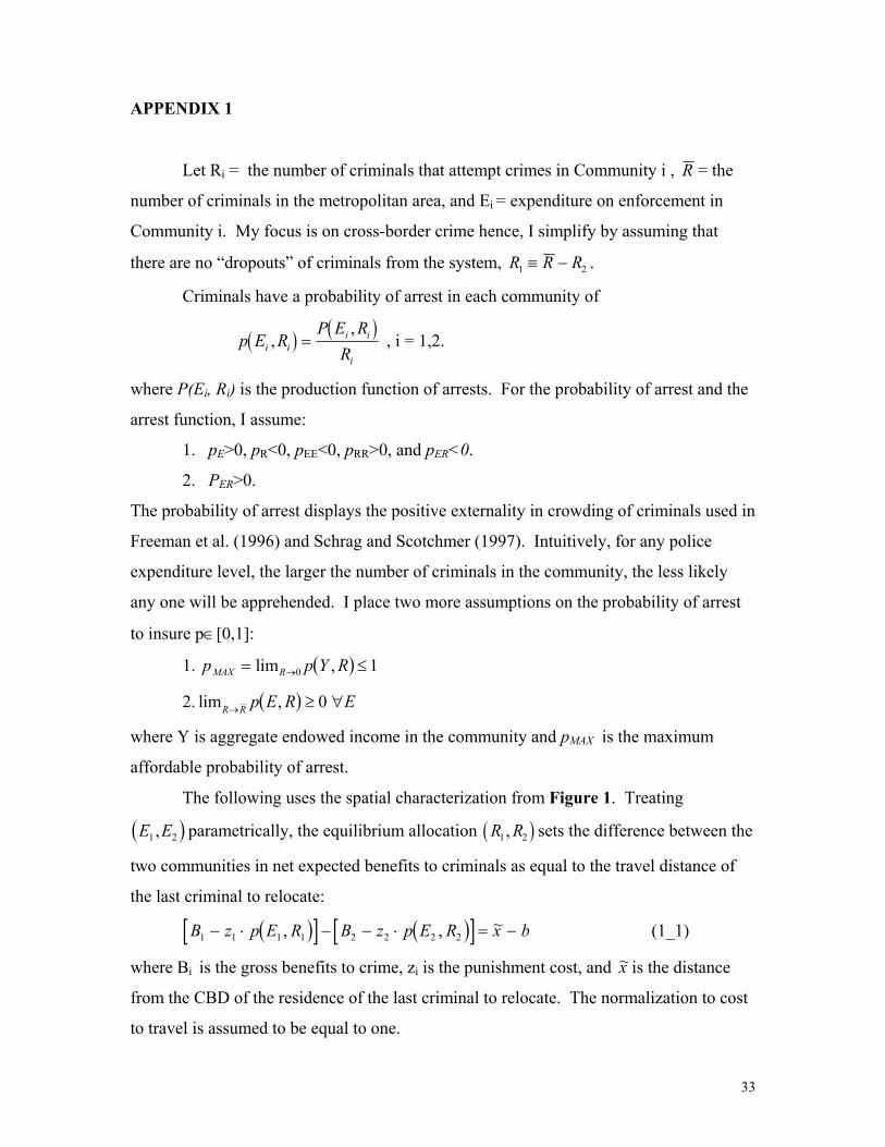
APPENDIX 1

Let Ri = the number of criminals that attempt crimes in Community i , R = the

number of criminals in the metropolitan area, and Ei = expenditure on enforcement in

Community i. My focus is on cross-border crime hence, I simplify by assuming that

there are no “dropouts” of criminals from the system, R R R1 2≡ − .

Criminals have a probability of arrest in each community of

( ) ( )p E RP E R

Ri ii i

i

,,

= , i = 1,2.

where P(Ei, Ri) is the production function of arrests. For the probability of arrest and the

arrest function, I assume:

1. pE>0, pR<0, pEE<0, pRR>0, and pER<0.

2. PER>0.

The probability of arrest displays the positive externality in crowding of criminals used in

Freeman et al. (1996) and Schrag and Scotchmer (1997). Intuitively, for any police

expenditure level, the larger the number of criminals in the community, the less likely

any one will be apprehended. I place two more assumptions on the probability of arrest

to insure p∈[0,1]:

1. ( ) limp p YMAX R= R ≤→0 1,

2. ( )lim R R p E R E→ ≥ ∀, 0

where Y is aggregate endowed income in the community and pMAX is the maximum

affordable probability of arrest.

The following uses the spatial characterization from Figure 1. Treating

parametrically, the equilibrium allocation (E E1 2, ) ( )R R1 2, sets the difference between the

two communities in net expected benefits to criminals as equal to the travel distance of

the last criminal to relocate:

( )[ ] ( )[B z p E R B z p E R x1 1 1 1 2 2 2 2− ⋅ − − ⋅ = −, , ~] b (1_1)

where Bi is the gross benefits to crime, zi is the punishment cost, and ~x is the distance

from the CBD of the residence of the last criminal to relocate. The normalization to cost

to travel is assumed to be equal to one.

33

Newlon (1999) demonstrated that (1_1) is stable. The equilibrium is also unique

when and b K p MAX< ⋅2 2 M b K p MAX− < ⋅1 1 .

Let the distribution of criminal residences be g(x) where x is the distance from

the CBD. Figure 1 presents an example of g(x). The distribution is assumed to be

uniform or decreasing in distance from the CBD. To simplify the exposition, let B1=B2

and z1=z2=z. Using (1_1) and the cumulative distribution function of criminal

residences, G(x), crime in Community 1 is

( ) ( )[[R R G z p E R p E R b1 2 2 1= ⋅ ⋅ − +, , ] ]1 (1_2)

and in Community 2 is

( ) ( )[[R R R G z p E R p E R b2 2 2 1= − ⋅ ⋅ − +, , ] ]1 . (1_3)

34

APPENDIX 2: Derivation of Predictions for Aggregate Expenditure.

This section characterizes the relationship between the travel distance in the

municipalities and the aggregate per capita expenditure (ej) on policing for a metropolitan

area. The results are presented in two propositions. The first proposition looks at how a

change in only one municipality’s travel distance affects expenditure at the metropolitan

level, ej. In deriving this result I assume the other municipalities’ travel distances are

held fixed. This allows me to focus in on the size of the effect of spillover at the

municipal level.

In the second proposition, municipal travel distances are a function of a fixed land

area for the metropolitan area. Therefore if one municipality’s travel distance changes, it

affects the TDij of all the other municipalities. Here I am testing for an average travel

distance effect on ej.

Both predictions used to test for the effect of spillover crime on police

expenditure are derived from the same key municipal result. In Newlon (2000), it was

shown for the Open Community Case (OCC), that if municipal travel distance to another

community (TDij) increases then municipal expenditure on enforcement (Eij) will

decrease,

0<ij

ij

dTDdE

for i = 1,2. (A2_1)

The negative relationship between expenditure and travel distance is a result of travel

distance’s effect on the price of safety in the community. As the travel distance in the

community increases, there is an increase in the price of safety. Intuitively, the price of

safety increases because the number of criminals exported per dollar has decreased with

the increase in the travel distance.

On the other hand, in the Closed Community Case (CCC), because criminal

activities are not cross jurisdictional, travel distance does not affect the safety of voters

and there is no relationship between Eij and TDij :

35

0=ij

ij

dTDdE

for i = 1,2. (A2_2)

Throughout the analysis presented in this appendix I treat communities as

“islands” such that no one lives near the boundaries, but criminals still differ in their

inclination to commute to commit crimes. This treatment allows the empirical model to

correspond to the theoretical model. A complete theoretical modeling of the effect of a

change in TDij includes all variables that depend on the placement of municipal

boundaries (b). But the estimation equation controls for municipal population (Nij) ,

resident criminals ( )ijR , median income ( )ijy~ and other variables that change with TDij.

Therefore to be consistent, the theoretical predictions assume these variables are fixed.

PART 1: Municipal Travel Distance and Metropolitan Expenditure per capita.

In Proposition 1, presented below, I assume that the travel distance in

municipalities is independent:

0 1

2 =j

j

dTDdTD

. (A2_3)

This assumption requires land area not fixed be fixed. One can imagine the change in the

travel distance occurs in the boundary municipalities.

Proposition 1: If travel distance in municipalities vary independently,

Then only in OCC does 0<ij

j

dTDde

for any i = 1,2.

The basis of this result is that expenditure per capita at the metropolitan level decreases

with an increase in the travel distance of one municipality only in the OCC because in the

CCC, (A2_2) holds.

36

Proof:

Aggregating municipal expenditure up to per capita expenditure in metropolitan

area j gives me

j

jjj N

EEe 21 +

= (A2_4)

where Nj is the total population in the metropolitan area.

Next I differentiate equation (A2_4) with respect to TDij. For expositional

purposes I use TD1j. The use of community 1’s travel distance is arbitrary; the result is

the same for either community’s travel distance.

+++=

j

j

j

j

j

j

j

j

j

j

j

j

jj

j

dTDdTD

dTDdE

dTDdTD

dTDdE

dTDdE

dTDdE

NdTDde

1

2

2

2

1

2

2

1

1

2

1

1

1

1 .

Using the result in (A2_3), the above derivative simplifies to

+=

j

j

j

j

jj

j

dTDdE

dTDdE

NdTDde

1

2

1

1

1

1 (A2_5)

A change in TD1j does not directly affect E2j, it changes only in reaction to a change in

R1j. To demonstrate this, I start by expanding j

j

TDE

1

2∂ and rewriting (A2_5) to get

⋅⋅+=

j

j

j

j

j

j

j

j

jj

j

dTDdR

dRdR

dRdE

dTDdE

NdTDde

1

1

1

2

2

2

1

1

1

1 (A2_6)

37

i. In the CCC, clear 01

=j

j

dTDde

because from (A2_2) 01

1 =j

j

dTDdE

and

01

2 =j

j

dRdR 27.

ii. In the OCC, because jj RRR 21 += , spill-ins are one-to-one with spill-outs

and 11

2 −=j

j

dRdR

. Using this information, (A2_6) can be rewritten as

01

1

1

2

2

1

1

1

<

⋅−=

j

j

j

j

j

j

jj

j

dTDdR

dRdE

dTDdE

NdTDde

(A2_7)

From (A2_1) 01

1 <j

j

dTDdE

and from Newlon (2000), I have 02

2 >j

j

dRdE

. The sign of

j

j

dTDdR

1

1 is best demonstrated in two parts.

i. Assume at a given equilibrium ( )*2

*1 , jj EE , that 21 pp ≤ .

In this case, community 2 is exporting criminal activity into community 1, therefore the crime equation for community 1 is

( 122

211 pp

TDR

CRRj

jjj −⋅+= ) . (A2_8)

Differentiating (A2_8) gives 01

1 =j

j

dTDdR

.

ii. Assume at a given equilibrium ( )*2

*1 , jj EE , that . 21 pp >

27 Although jj RRR 21 += , in the CCC jj RR 11 ≡ and jj RR 22 ≡ . Because both jR1 and jR 2

are fixed, it follows that 01

2 =j

j

dRdR

.

38

In this case the exporter is community 1 and thus their crime equation is

( 121

111 pp

TDR

CRRj

jjj −⋅+= ) . (A2_9)

Differentiating (A2_9) results in

( )

0

12

2

1

1

1

1

1221

1

1

1 >

∂∂

+∂∂

+

−⋅−

=

jjj

j

j

j

j

j

Rp

Rp

TDR

ppTDR

C

dTDdR

,

because the denominator is positive, see Newlon(2000).

#

PART 2: Average Municipal Travel Distance and Metropolitan Expenditure per capita.

For Proposition 2, I assume that land area (M) is fixed. This implies that municipal travel

distance is not independent and can be characterized as functions of each other,

TDij(TDkj) where i ? k. In the 2-community model, travel distances combine to equal the

total land area,

MTDTD jj =+ 21 . (A2_10)

Differentiating (A2_10) results in the following relationship between travel distances,

12

1 −=j

j

dTDdTD

. (A2_11)

I define the average travel distance (ATDj) in the metropolitan area as a population-

weighted average

39

j

jj

j

jjj N

NTD

NN

TDATD 22

11 += . (A2_12)

Proposition 2: If municipal travel distances vary inversely,

Then only in the OCC does 0≠ij

j

dATDde

for any i = 1,2.

Proof:

The derivative of ej with respect to ATDj is composed of two parts28

j

j

j

j

j

j

j

j

j

j

dATDdTD

dTDdTD

dTDde

dTDde

dATDde 1

1

2

21

⋅

⋅+=

Simplifying using (A2_11), I get

j

j

j

j

j

j

j

j

dATDdTD

dTDde

dTDde

dATDde 1

21

⋅

−= . (A2_13)

Expanding results in (A2_13) gives

j

j

j

j

j

j

j

j

j

j

jj

j

dATDdTD

dTDdE

dTDdE

dTDdE

dTDdE

NdATDde 1

2

1

1

2

2

2

1

11⋅

−+

−= , (A2_14)

where 021

1

>−=j

j

j

j

j

j

NN

NN

dTDdATD

jj NN 21 >

due to the assumption that the central city has the larger

population, .

40

In equation (A2_14), the sign of the derivatives ij

ij

dTD

dE in

−

j

j

j

j

dTDdE

dTDdE

2

2

1

1 are

the same. The same holds for the sign of the derivatives kj

ij

dTDdE

, where i ? k, in

−

j

j

j

j

dTDdE

dTDdE

2

1

1

2 . These two results imply for the OCC that the direction of the

relationship between ej and ATDj is ambiguous. Both parts of the derivative can be

either negative or positive, depending on the relative size of the expenditure response in

the communities. The results in the computational analysis presented Figure2 show that

expenditure is increasing in average travel distance for a range of boundary

specifications. There is no ambiguity in the CCC because ij

ij

dTD

dE=

kj

ij

dTDdE

=0 for i = 1, 2

and where i ? k.

#

28 I chose to differentiate with respect to TD1j because it has a positive relationship to ATDj. To use TD2j would not change the conclusion of the proof.

41

APPENDIX 3

A computational model allows the development of a more complete picture of the

relationship between relative community characteristics and expenditure levels, and in

turn, relative safety and crime rates. I have strived, whenever possible, to calibrate the

computational model to existing empirical evidence. This appendix discusses the

calibration of the utility and production of arrests functions.

The calibration strategy is based on a symmetric equilibrium. The symmetry of

communities required for such an equilibrium reduces the calibration to only one of the 2

communities. An added benefit of the symmetric equilibrium is that it results in no

spillover between the communities, thus allowing for the calibration of the number of

resident criminals, a variable impossible to get accurate data for. The calibration

strategy dictates the choice of the data source. Municipal level data are likely to reflect

spillover if the municipality is not surrounded by perfectly symmetric communities.

Therefore, national-level data and scale-free empirical results offer the best

approximation to a symmetric equilibrium because they best approximate a zero-

spillover situation without eliminating expenditure distortions. Where necessary, scale-

free specifications are utilized to ameliorate the size of national data. Finally, it can be

shown that the parameters that cannot be set with data are not pivotal since the result of

increasing per capita expenditure in Figure 2 exists for a wide range of values for these

parameters.

Specification, Data and Results:

Most of the calibration data used are from 1990. The exceptions are published

results, often involving data spanning many years. A community has a population of

248,728,000 persons and a median income of $29,243 (Statistical Abstract, 1992). The

expenditure per person on local, state, and federal police is $127.87 (Statistical Abstract,

1993).29 The form of the state-dependent utility function is

( ) ( ) ( ) ( )U y e S S y e S y e BA A− = ⋅ − + − ⋅ − − −, ( )1 1 .

29 The lion's share of that expenditure came in at the local level at $92.80 per person (Statistical Abstract, 1993).

42

In addition to the expenditure per capita, I also use the estimate of .71 for the income

elasticity of demand for enforcement from Bergstrom and Goodman (1973) to calibrate

the utility function. The resulting calibration of the utility function is: A = 0.5019 and B

= 1720.70.

In the computational program, I allow for the justice system’s effect on the

probability of criminal punishment. In 1990, the total number of crimes cleared by arrest

is 2,909,137 (Sourcebook of Criminal Justice Statistics, 1998). Data on the percent of

arrests leading to conviction or guilty pleas is imperfect but upper estimates from Mulkey

(1975) place it at 45.7%. I set the probability of punishment given arrest (f) at 45%. The

arrests function is Cobb-Douglas with constant returns to scale. For per capita

punishment or apprehension, the functional form is

( )ρβ

αα= ⋅

−f e r 1 .

The calibration of the punishment equation results in a low enforcement elasticity

of α = 0.1944, making the production of arrests highly dependent on the number of

criminals in the community. The parameter (β) adjusts the expenditure level to reflect

the officers and equipment purchased, and put the expenditure variable in units close to

those of the resident criminal per capita. The calibrate value is β = 19,736.51.

The actual number, rather than the reported number, of crimes, sets the safety

level. I use the percent of crimes reported to police, approximately 40% (Bureau of

Justice Statistics, 1994), to adjust the reported crime rate, .054, for index crimes (murder,

rape, assault, robbery, burglary, larceny, and motor vehicle theft) to the actual crime rate,

(ac) of .135 (Sourcebook of Criminal Justice Statistics, 1998). In addition I remove the

restriction that criminals commit only one crime. In the computational model, I assume

criminals commit K crimes if they are not arrested, and otherwise commit ~K crimes

before arrest. The safety equation is

( )( )S ac K r K= − = − ⋅ − + ⋅1 1 ρ ρ~ .

I use empirical results from Levitt (1996) to calibrate the actual crime rate. Levitt

estimated that an average criminal released from prison commits 15 crimes. I interpret

this result to be the average of two types of criminals: 1) those that remain free during the

43

following year, and 2) those that are re-arrested. I am thus able to calibrate the criminal's

effort level (K) and the number of criminals residing in the community, r . Because I do

not have data on the average number of crimes that criminals commit before arrest, I set

the average as at the value of zero used in the theoretical analysis. Thus criminals are

apprehended attempting their first crime. The results in Figure 2 are robust to a full

range of pre-arrest crimes from almost all K to no crimes actually accomplished. The

calibrated number of crimes committed on average by an unarrested criminal is 22.33.

The per capita number of criminals residing in the community is 0.0102.

Finally, I have chosen not to use the elasticity of crime rate with respect to the

officer rate reported in Levitt (1997). Having found that Levitt's estimate implies a large

difference between the open- and closed-community expenditure levels, I use instead a

lower elasticity of –0.2418 in order to dampen the spillover effect. As such, communities

in the CCC spend $61.44 per person; starting from the symmetric equilibrium, this is a

little less than half of the OCC expenditures.

The choice of the length of the symmetric communities, or M in Figure 1, is not

as important as its relation to the gross cost of punishment, z (see Appendix 1). The

resulting calibration is the same for any fixed ratio of punishment to travel cost (z/b)

where b is the length of one community. I use a ratio of 1 so that the cost to punishment

is larger than the relocation distance for all but those with the farthest distance to travel.

44

APPENDIX 4

The system of structural equations is

e f r y Xj j j j j j= ( , , , , )∆ Ω j+ ε (A_4.1)

and

(r g e X Wj j j j j j= , , , ,∆ Ω η) j+

j+

(A_4.2)

( )PD h AD Xj j j= , ν (A_4.3)

where j indexes the metropolitan area, e is the officers rate, r is the crime rate, X is a

vector of demographic characteristics, PD is the population-based average distance

measure, AD is the area-based average distance measure, W is a vector of temperature

measures, ∆ is a measure of costs to criminals of relocation of activity, and Ω is the

spatial costs of policing.

45

APPENDIX 4

The two main types of numerical identification codes were created separately by the

Census Bureau and the Federal Bureau of Investigation. The demographic and municipal

structure data comes from the 1990 Census STF3A files. Impediments data also use

census codes, despite having been collected by the National Geographic Survey for their

Geographic Names Information System. Crime and enforcement data were collected by

the FBI in cooperation with local and state law enforcement at the jurisdictional level.

The Inter-university Consortium on Political and Social Research (ICPSR) provided a

translation algorithm between the two types of code at the county level. They are

currently working on a municipal-to-jurisdictional bridge.

Impediments: The structure of the data makes it nearly impossible to get a count of

linear features for each county from the raw data publicly available to researchers. The

Geographic Names Information System proved invaluable by transforming the county

level data for streams, ridges, and bridges.

Temperature: The variables collected for temperature are the normals for monthly and

annual temperature, heating degree days and cooling degree days. Normals are 30-year

average values from the years 1961-1990. Cooling degree days is the sum of the positive

difference, respectively, between daily average temperature and 65 degrees. They are

accumulated from January 1 to December 31. All of the data comes from the National

Oceanic and Atmospheric Administrations (NOAA) national climactic data center. Some

of the data are extracted from the Comparative Climatic Data File. The rest of the data

are collected by hand from the normals files for all stations across the United States.

Unfortunately, these files do not identify stations by name. I use the NCDC station

locator web site to match the cooperative station number with the location of the station.

46

BIBLIOGRAPHY Barr, R., and Pease, K. “Crime Placement, Displacement and Deflation,” in M. Tonry and

N. Morris, eds., Crime and Justice: A review of research, Vol.12. Chicago, IL: University of Chicago Press, 1990.

Bergstrom, Theodore C., and Goodman, Robert P. “Private Demands for Public Goods.”

American Economic Review, June 1973, 63(3), pp. 280-96. Brantingham, Patricia L., and Brantingham, Paul J. “Mobility, Notoriety and Crime: A

Study in Crime Patterns of Urban Nodal Points.” Journal of Environmental Systems, 1984, 11, pp. 89-99.

Brantingham, Patricia L., and Brantingham, Paul J. Patterns in Crime. New York,

NY: MacMillan, 1984. Brantingham, Patricia L., and Brantingham, Paul J. “Environment, Routine and Situation:

Toward a Pattern Theory of Crime.” in Clark and Felson eds., Routine Activity and Rational Choice: Advances in Criminological Theory, 5, New Brunswick, NJ: Transaction Books, 1993.

Buettner, Thiess, and Spengler, Hannes. “Criminal Mobility and Neighborhood Effects:

An Empirical Study of the Determinants of Crime.” Working Paper, April, 2001. Bureau of Justice Statistics. Criminal Victimization in the United States. Washington,

DC : Department of Justice, 1994. Cameron, Samuel. “The Economics of Crime Deterrence: A Survey of Theory and

Evidence.” Kyklos, May 1988, 41(2), pp. 301-23. Cohen, L.E., Nisbett, R. E.; Bowdle, B. F., and Schwarz, N. “Insult, Aggression, and the

Southern Culture of Honor: An ‘Experimental Ethnography.’” Journal of Personality & Social Psychology, 70(5), May 1996, pp. 945-960.

Cohen, L.E., and Felson, M. "Social Change and Crime Rate Trends: A Routine Activity

Approach." American Sociological Review, 1979, 44, pp. 588-607. Capone, D.C., and Nichols, W.W., Jr. “Urban Structure and Criminal Mobility.”

American Behavioral Scientist, November-December 1976, 20, pp. 199-213. Corman, Hope, and Mocan, Naci H. “A Time-Series Analysis of Crime and Drug use in

New York City.” National Bureau of Economic Research, Working Paper, February 1996.

47

Deutsch, Joseph, Hakim, Simon and Weinblatt, J. “Interjurisdictional Criminal Mobility: A Theoretical Perspective,” Urban Studies, November 1984, 21(4), pp. 451-58.

Dodge, Richard W. The Seasonality of Drime Victimization. Washington, DC: U.S. Dept.

of Justice, Bureau of Justice Statistics, 1988. Eide, Erling; Aasness, Jorgen and Skjerpen, Terje. Economics of Crime: Deterrence and

the Rational Offender. Amsterdam; New York: Elsevier, 1994. Epple, Dennis; Filimon, Radu and Romer, Thomas. “Equilibrium Among Local

Jurisdictions: Towards an Integrated Treatment of Voting and Residential Choice.” Journal of Public Economics, August 1984, 24(3), pp.281-308.

Epple, Dennis and Romer, Thomas. “On the Flexibility of Municipal Boundaries.”

Journal of Urban Economics, 1989, 26, pp. 307-319. Fabrikant, Richard. “Interjurisdictional Spillovers of Urban Police Services: Comment.”

Southern Economic Journal, January 1980, 46(3), pp. 955-961. Felson, Marcus. Crime and Everyday Life, Vol. 2. USA: Pine Forge Press, 1998. Fisher, Franklin and Nagin, Daniel. “On the Feasibility of Identifying the Crime Function

in a Simultaneous Equations Model of Crime and Sanctions,” in Alfred Blumstein, Daniel Nagin, and Jacqueline Cohen, eds., Deterrence and Incapacitation: Estimating the Effects of Criminals Sanctions on Crime Rates. Washington, DC: National Academy of Sciences, 1978.

Freeman, Scott; Grogger, Jeffrey and Sonstelie, Jon. “The Spatial Concentration of

Crime.” Journal of Urban Economics, September 1996, 40(2), pp. 216-31. Mulkey, Michael A. Chapter 11, in John A. Gardiner, and Michael A. Mulkey, eds.,

Crime and Criminal Justice : Issues in Public Policy Analysis. Lexington, MA: Lexington Books, 1975.

Hesseling, R. B. “Displacement: A Review of the Empirical Literature,” in R. V. Clarke,

ed., Crime Prevention Studies, Vol. 3. Monsey, NY: Criminal Justice Press, 1993. Hakim, Simon; Ovadia, Arie; Sagi, Eli and Weinblatt, J. “Interjurisdictional Spillover of

Crime and Police Expenditure.” Land Economics, May 1979, 55, pp.200-212. Hoxby, Caroline M. “Does Competition Among Public Schools Benefit Students and

Taxpayers? Evidence from Natural Variation in School Districting.” National Bureau of Economic Research, Working Paper, 1997.

Levitt, Steven. “The Effect of Prison Population Size on Crime Rates: Evidence from

Prison Overcrowding Litigation.” Quarterly Journal of Economics, May 1996,

48

111(2), pp.319-351. Levitt, Steven. “Using Electoral Cycles in Police Hiring to Estimate the Effect of Police

on Crime.” The American Economic Review, June 1997, 87(3), pp. 270-290. Marceau, Nicolas. “Competition in Crime Deterrence.” Canadian Journal of Economics,

November 1997, 30(4), pp. 844-854. Mehay, Stephan L. “Interjurisdictional Spillovers of Urban Police Services.” Southern

Economic Journal, January 1977, 43(3), pp. 1352-1359. Newlon, Elizabeth. “Law Enforcement by Competing Jurisdictions When Criminals are

Mobile.” Carnegie Mellon University, Working Paper, June 1998. Nisbett, Richard E. and Cohen, Dov. “Culture of honor: The Psychology of Violence in

the South.” New Directions in Social Psychology. Boulder, CO: Westview Press, 1996.

Olligschlaeger, Andreas M. “Spatial Analysis of Crime Using GIS-Based Data: Weighted

Spatial Adaptive Filtering and Chaotic Cellular Forecasting with Applications to Street Level Drug Markets.” Carnegie Mellon University, Working Paper, May 1997.

Pittsburgh Post Gazette. “Drugs, Violence Become a Habit in Wilkinsburg.” Pittsburgh

Post Gazette, February 23, 1992. Pope, C.E. “Patterns in Burglary: An Empirical Examination of Offense and Offender

Characteristics.” Journal of Criminal Justice, 1980, 8(1), pp. 39-51. Poyner, B. “What works in crime prevention: An Overview of Evaluations,” in R. V.

Clarke ed., Crime prevention studies, Vol. 3. Monsey, NY: Criminal Justice Press, 1993.

Reppetto, T.A. “Crime Prevention and the Displacement Phenomenon.” Crime and

Delinquency, April 1976, 22, pp. 166-177. Shaw, Clifford R. Delinquency Areas. Chicago: University of Chicago Press, 1929. Schmid, C. F. “Urban Crime Areas: Part 1.” American Sociological Review, 25, pp. 166-

177. Schrag, Joel and Scotchmer, Suzanne. “The Self-Reinforcing Nature of Crime.”

International Review of Law and Economics, September 1997, 17 (3), pp. 325-35. Sourcebook of Criminal Justice Statistics. Washington, DC: U.S. Dept. of Justice, Bureau

of Justice Statistics, 1990, 1997, & 1998.

49

Statistical Abstract of the United States. Washington, DC: U.S. Dept. of Commerce,

Bureau of the Census, 1992 & 1993. Tiebout, C. “A Pure Theory of Local Expenditures.” Journal of Political Economy, 1953,

64, pp. 416-424.

50

Table 1: Summary Statistics

Variable Mean Median Std. Dev. Maximum Minimum Population 685,125.30 240,282.00 1,663,775.00 18,087,251.00 56,735.00 Officer Rate 208.00 177.50 256.98 4,127.55 70.76 Crime Rate 5,632.43 5,462.05 1,998.09 11,974.71 351.15 Violent Crime Rate 576.21 535.02 342.45 1,793.72 46.14 Property Crime Rate 5,056.19 4,967.01 1,756.81 11,375.22 303.31 Average Distance to a Border (in miles) 1.80 1.51 1.02 8.15 0.62 Number of Streams 188.23 106.50 221.98 1,411.95 0.00 Number of Ridges 11.41 2.00 30.54 303.00 0.00 Number of Bridges 7.71 3.00 14.31 102.00 0.00 Number of Annual Cooling Days 1,437.99 971.03 1,141.00 4,305.00 51.00 Average Temperature in Winter Months 37.29 12.55 36.63 68.27 8.33 Median Income 28,146.63 27,517.00 4,416.45 42,250.00 16,703.00 Within-City Variance in Income 0.44 0.43 0.11 1.25 0.24 Percent Black 0.10 0.07 0.10 0.46 0.00 Percent Hispanic 0.07 0.02 0.13 0.94 0.00 Percent Female-Headed Households 0.14 0.12 0.05 0.35 0.06 Percent Older Than 24 Years 0.63 0.63 0.04 0.78 0.43 Percent With a College Degree 0.24 0.23 0.06 0.42 0.11 Mean Public Assistance Per Household 3,784.51 3,678.44 764.52 7,300.10 2,592.55 Percent of Population With Income Above $100,000 0.03 0.03 0.01 0.10 0.01 Percent of Population in the Labor Force 0.65 0.65 0.05 0.79 0.50

All rates are per 100,000 residents. The sample used is a set of 255 MSAs . The mean public assistance per household is in 1983 dollars.

51

Table 2: First-Stage Results for Crime Rate

Dependent Variable: Log of the Crime Rate

White Heteroskedasticity-Consistent Standard Errors & Covariance All rates are per capita

OLS Std. Error Weather Instruments:

Log of the Number of Cooling Days 0.060 0.012 Log of the Average Temperature in Winter 0.276 0.022

Income Measures:

Log of the Median Household Income -0.122∆ 0.078 Within-City Variance in Income -0.002∆ 0.051 Percent of Population with Income Over 100,000 3.333 0.859

Spatial Characteristics:

Log of Land Area -0.079 0.013 Herfindahl Index -0.933 0.154 Log of Area-Based Average Travel Distance 0.325 0.029 Log of Municipal Travel Distance 0.024 0.003 Log of Population 0.007∆ 0.012 Log of the Number of Streams -0.041 0.011 Log of the Number of Ridges -0.022 0.003 Log of the Number of Bridges 0.013 0.003 CMSA Indicator 0.029 0.008

Demographic Variables:

Percent Black 0.321 0.093 Percent Hispanic -0.100∆ 0.138 Percent Female Headed Households 5.470 0.346 Percent of Population over 24 0.958 0.202 Percent with a College Degree 1.265 0.127 Log of the Mean Public Assistance Per Household -1.658 0.348 Percent of Labor Force Employed -4.348 0.506 Percent of Population in the Labor Force 2.464 0.174

Division Indicators:

East North Central Division 0.251 0.013 West North Central Division 0.239 0.016 South Atlantic Division 0.001∆ 0.013 East South Central Division -0.017∆ 0.018 West South Central Division 0.083 0.023 Mountain Division 0.045∆ 0.050 Pacific Division 0.021∆ 0.025 Constant (Middle Atlantic Division) -1.616∆ 1.006

F-statistic 682.322 R-squared 0.727 Adjusted R-squared 0.726 S.E. of regression 0.198 All coefficients are significant at a p-value <.001 unless market with a ∆. Average distance is measured in miles. The mean public assistance per household is from 1983.

52

Table 3: Estimates for Municipal Travel Distance

Dependent Variable: Log of Local and County Officer Rate

Observations: 9272 All rates are per capita Instrumental Variables OLS 1 2

Log of Municipal Travel Distance (TDij) -0.001∆ -0.025 0.011

Endogenous Variables:

Crime Rate 0.286 0.152 0.156 Log of the Average Median Household Income 2.317 -5.020 -

Income Measures:

Log of the Median Household Income -2.134 4.919 0.091 Income Variance -0.060∆ 0.005 0.026 Percent of Population with Income Over 100,000 7.044 0.193 0.316

Spatial Characteristics:

Herfindahl Index 0.181 0.113 0.042 Log of Area-Based Average Travel Distance 0.186 0.183 0.256 Log of Population -0.064 -0.018 -0.161 Log of the Number of Streams 0.015 0.046 0.001 Log of the Number of Ridges -0.008 -0.105 -0.025 Log of the Number of Bridges 0.026 0.340 0.151 CMSA Indicator 0.096 0.310 0.149

Demographic Variables:

Percent Black 0.317 0.000 0.110 Percent Hispanic -0.234 -0.063 -0.073 Percent Female-Headed Households 2.708 0.298 0.226 Percent of Population Over 24 Years 0.092∆ 0.075 0.017 Percent with a College Degree 0.641 0.194 0.144 Log of Mean Public Assistance Per Household 2.323 0.211 0.164 Percent of Labor Force Employed 2.650 0.212 0.135 Percent of Population in the Labor Force -0.604 -0.057 -0.055

Division Indicators:

East North Central Division 0.118 0.171 0.194 West North Central Division 0.092 0.131 0.137 South Atlantic Division 0.041 -0.045 0.071 East South Central Division 0.017∆ -0.008 0.019 West South Central Division 0.058 0.052 0.086 Mountain Division -0.064 -0.024 -0.011 Pacific Division -0.451 -0.321 -0.272 Constant (Middle Atlantic Division) -9.841 -0.001 -0.003

R squared 0.788 0.827 0.748 Omnibus Test - 176.335 136.280 All coefficients are significant at a p-value <.001 unless market with a ∆. Average distance is measured in miles. The mean public assistance per household is from 1983.

53

Table 4: First-Stage Results for Crime Rates

Dependent Variable: Log of the Crime Rate

White Heteroskedasticity-Consistent Standard Errors & Covariance All rates are per capita

OLS Std. ErrorWeather Instruments:

Log of the Number of Cooling Days 0.059 0.012 Log of the Average Temperature in Winter 0.284 0.022

Income Measures:

Log of the Median Household Income -0.131∆ 0.078 Within-City Variance in Income -0.017∆ 0.052 Percent of Population with Income Over 100,000 3.412 0.865

Spatial Characteristics:

Herfindahl Index -0.969 0.156 Log of Area-Based Average Travel Distance 0.347 0.030 Log of Population 0.006∆ 0.012 Log of the Land Area -0.081 0.013 Log of the Number of Streams 0.012 0.003 Log of the Number of Ridges -0.023 0.003 Log of the Number of Bridges -0.040 0.011 CMSA Indicator 0.022 0.008

Demographic Variables:

Percent Black 0.331 0.093 Percent Hispanic -0.075∆ 0.138 Percent Female Headed Households 5.542 0.344 Percent of Population over 24 0.963 0.202 Percent with a College Degree 1.302 0.126 Log of the Mean Public Assistance Per Household -1.752 0.347 Percent of Labor Force Employed 2.464 0.174 Percent of Population in the Labor Force -4.394 0.509

Division Indicators:

East North Central Division 0.260 0.013 West North Central Division 0.245 0.016 South Atlantic Division 0.004 0.013 East South Central Division -0.008 0.018 West South Central Division 0.084 0.023 Mountain Division 0.056 0.050 Pacific Division 0.026 0.025 Constant (Middle Atlantic Division) -1.498 1.014

F-statistic 695.498 0.000 R-squared 0.725 Adjusted R-squared 0.724 S.E. of regression 0.198

All coefficients are significant at a p-value <.001 unless market with a ∆. Average distance is measured in miles. The mean public assistance per household is from 1983.

54

Table 5: First-Stage Results for Average Travel Distance

Dependent Variable: Log of the Distance Measure

White Heteroskedasticity-Consistent Standard Errors & Covariance All rates are per capita

OLS Std. Error Travel Distance Instruments:

Herfindahl Index -0.985 0.082 Log of Area-Based Average Travel Distance 0.785 0.020

Weather Instruments:

Log of the Number of Cooling Days 0.054 0.009 Log of the Average Temperature in Winter 0.002∆ 0.019

Income Measures:

Log of the Median Household Income -1.196 0.071 Within-City Variance in Income -0.663 0.051 Percent of Population with Income Over 100,000 8.456 0.746

Spatial Characteristics:

Log of Population 0.098 0.007 Log of the Land Area -0.178 0.011 Log of the Number of Streams 0.000∆ 0.003 Log of the Number of Ridges -0.019 0.003 Log of the Number of Bridges 0.071 0.008 CMSA Indicator -0.115 0.009

Demographic Variables:

Percent Black 0.495 0.074 Percent Hispanic 0.636 0.085 Percent Female Headed Households 1.371 0.358 Percent of Population over 24 1.112 0.109 Percent with a College Degree 0.616 0.069 Log of the Mean Public Assistance Per Household -0.869∆ 0.319 Percent of Labor Force Employed 0.881∆ 0.126 Percent of Population in the Labor Force 2.238 0.476

Division Indicators:

East North Central Division 0.273 0.008 West North Central Division 0.180 0.012 South Atlantic Division 0.075 0.009 East South Central Division 0.370 0.014 West South Central Division 0.271 0.020 Mountain Division 0.354 0.034 Pacific Division 0.266 0.027 Constant (Middle Atlantic Division) 7.755 0.794

F-statistic 1236.517 0.000 R-squared 0.824 Adjusted R-squared 0.823 S.E. of regression 0.182 All coefficients are significant at a p-value <.001 unless market with a ∆. Average distance is measured in miles. The mean public assistance per household is from 1983.

55

Table 6: Estimates from Average Travel Distance Dependent Variable: Log of Local and County Officer Rate

Observations: 9272 All rates are per capita Instrumental

Variables OLS 1 2

Endogenous Variables:

Log of the Distance Measure 0.061 0.824 0.820 Crime Rate 0.295 -0.340 -0.370 Log of the Average Median Household Income 2.587 2.883 -

Income Measures:

Log of the Median Household Income -2.222 -2.423 0.313 Income Variance 0.127 0.165 0.138 Percent of Population with Income Over 100,000 5.034 0.268 0.256

Spatial Characteristics:

Log of Population -0.099 -0.427 -0.342 Log of Land Area 0.044 -0.039 -0.071 Log of the Number of Streams 0.005 -0.124 -0.102 Log of the Number of Ridges -0.008 -0.029 -0.092 Log of the Number of Bridges 0.019 0.105 0.210 CMSA Indicator 0.092 0.153 0.252

Demographic Variables:

Percent Black 0.473 0.176 0.110 Percent Hispanic -0.092∆ -0.127 -0.125 Percent Female-Headed Households 2.707 0.295 0.366 Percent of Population Over 24 Years 0.374 -0.009 0.034 Percent with a College Degree 0.812 0.112 0.128 Log of the Mean Public Assistance Per Household 1.292 0.065 0.071 Percent of Labor Force Employed 1.288 -0.054 -0.013 Percent of Population in the Labor Force -0.837 0.009 0.017

Division Indicators:

East North Central Division 0.107 0.136 0.120 West North Central Division 0.089 0.137 0.123 South Atlantic Division 0.093 0.042 -0.039 East South Central Division 0.067 -0.143 -0.166 West South Central Division 0.113 -0.017 -0.039 Mountain Division 0.099 -0.084 -0.091 Pacific Division -0.294 -0.329 -0.354 Constant (Middle Atlantic Division) -10.214 0.000 0.009

R squared 0.775 0.871 0.872 Omnibus Test - 13.477 44.454 All coefficients are significant at a p-value <.001 unless market with a ∆. Average distance is measured in miles. The mean public assistance per household is from 1983.