spice like sparse transient analysis
TRANSCRIPT

SPICE Like Sparse Transient Analysis
by
SONALI R. LUNIYA
A thesis submitted to the Graduate Faculty ofNorth Carolina State University
in partial fulfillment of therequirements for the Degree of
Master of Science
COMPUTER ENGINEERING
Raleigh
2002
APPROVED BY:
Chair of Advisory Committee

Abstract
LUNIYA, SONALI. SPICE Like Sparse Transient Analysis. (Under the direc-tion of Michael B. Steer)
A state variable transient circuit analysis using sparse matrices is devel-
oped. The equations are formulated using time discretization based on New-
ton’s iterative method of equations of the nonlinear part of the circuit. The
system thus formed is an algebraic system of linear equations. The program
uses advanced numerical techniques, such as automatic differentiation for cal-
culating the Jacobian of the system. The program is tested by simulating a
Soliton line and a Wideband amplifier. The results of this analysis is compared
to those obtained from SPICE, and conclusions are made.

ii
Biographical Summary
Sonali R. Luniya was born on 27th August, 1978 in Pune, India. She
received a degree in Computer engineering in 2000 from the Pune Institute of
Computer Technology in Pune, India. From June 1999 to May 2000 she worked
as an intern with Parametric Technologies, Pune, India. She was admitted to
North Carolina State University in Spring 2001 in the Master of Computer
Engineering program. Her interests are in the fields of analog circuit design
and computer-aided analysis of circuits.

iii
Acknowledgments
I would like to express my sincere gratitude to my advisor, Dr. Michael
Steer for giving me an opportunity to work with his research group. It was
a great privilege to be a part of his NeoCAD research program. I would also
like to thank Dr. Griff Bilbro and Dr. Paul Franzon for serving on my thesis
committee.
My special thanks to Dr. Carlos Christofferson, for helping me understand
f REEDATM. His knowledge about f REEDATM provided me lots of tips along
the way. A very big thanks to all my graduate colleagues and friends. First
to Shubha Vijaychand and Houssam Kanj who helped me understand the
different analyses implemented in f REEDATM. To Jayanthi Suryanarayanan
and Rachana Shah, who helped me write this report. And to everyone else in
EGRC 410 and EGRC 412.
My special thanks to my parents whose foresight and sacrifice have put
me in a position to succeed. Last but not the least, I would like to thank my
loving husband, Abhi, for all his support, encouragement and care.

iv
Contents
List of Figures vi
1 Introduction 11.1 Motivation . . . . . . . . . . . . . . . . . . . . . . . . . . . . . 11.2 Thesis Overview . . . . . . . . . . . . . . . . . . . . . . . . . . 21.3 Original Contributions . . . . . . . . . . . . . . . . . . . . . . 3
2 Literature Review 42.1 Introduction . . . . . . . . . . . . . . . . . . . . . . . . . . . . 42.2 Nodal Analysis . . . . . . . . . . . . . . . . . . . . . . . . . . 4
2.2.1 Formulating Network Equations for Linear Circuits . . 52.2.2 Modified Nodal Analysis . . . . . . . . . . . . . . . . . 72.2.3 Nodal Analysis for Nonlinear Resistive Circuits . . . . 82.2.4 State Variable Formulation . . . . . . . . . . . . . . . . 9
2.3 Time Marching Transient Analysis . . . . . . . . . . . . . . . 102.3.1 Associated Discrete Model of a Linear Element . . . . 112.3.2 Associated Discrete Model of a Nonlinear Element . . . 132.3.3 Multi Terminal Elements . . . . . . . . . . . . . . . . . 15
2.4 Iteration Methods . . . . . . . . . . . . . . . . . . . . . . . . . 162.4.1 Fixed Point Method . . . . . . . . . . . . . . . . . . . 162.4.2 Newton Method . . . . . . . . . . . . . . . . . . . . . . 17
2.5 Summary . . . . . . . . . . . . . . . . . . . . . . . . . . . . . 18
3 SPICE-Like Sparse Transient Analysis 193.1 Nonlinear Equation Formulation . . . . . . . . . . . . . . . . . 19
3.1.1 Linear Network . . . . . . . . . . . . . . . . . . . . . . 20

v
3.1.2 Nonlinear Network . . . . . . . . . . . . . . . . . . . . 213.1.3 Error Function Formulation . . . . . . . . . . . . . . . 223.1.4 Sparse Matrix Formulation . . . . . . . . . . . . . . . . 243.1.5 Initial Operating Point . . . . . . . . . . . . . . . . . . 26
3.2 Implementation in f REEDATM . . . . . . . . . . . . . . . . . . 263.3 Support Libraries . . . . . . . . . . . . . . . . . . . . . . . . . 28
3.3.1 Solution to Sparse Linear Systems . . . . . . . . . . . . 283.3.2 Vectors and Matrices . . . . . . . . . . . . . . . . . . . 293.3.3 Automatic differentiation . . . . . . . . . . . . . . . . . 30
3.4 Summary . . . . . . . . . . . . . . . . . . . . . . . . . . . . . 32
4 Results 334.1 Introduction . . . . . . . . . . . . . . . . . . . . . . . . . . . . 334.2 Wide Band Amplifier . . . . . . . . . . . . . . . . . . . . . . . 334.3 Soliton Line . . . . . . . . . . . . . . . . . . . . . . . . . . . . 39
4.3.1 Circuit . . . . . . . . . . . . . . . . . . . . . . . . . . . 394.3.2 Results . . . . . . . . . . . . . . . . . . . . . . . . . . . 41
4.4 Summary . . . . . . . . . . . . . . . . . . . . . . . . . . . . . 45
5 Conclusions and Future Research 465.1 Conclusions . . . . . . . . . . . . . . . . . . . . . . . . . . . . 465.2 Future Research . . . . . . . . . . . . . . . . . . . . . . . . . . 47
A Computer Code 49
B Wideband Amplifier Netlist 57
C Soliton Line Netlist 59
Bibliography 65

vi
List of Figures
2.1 Associated discrete model of a two terminal element obtainedusing Backward Euler method. . . . . . . . . . . . . . . . . . . 13
3.1 Network with Nonlinear elements . . . . . . . . . . . . . . . . 203.2 General flow diagram of the program. . . . . . . . . . . . . . . 273.3 Automatic Differentiation . . . . . . . . . . . . . . . . . . . . 31
4.1 Wideband amplifier, from the MCNC benchmark suite with 11Gummel-Poon Bipolar Transistors. . . . . . . . . . . . . . . . 35
4.2 Output voltages at terminals out17, curve (a), and out16, curve(b), of the wideband amplifier simulated in f REEDATM. . . . . 36
4.3 Output voltages at terminals out17, curve (a), and out16, curve(b), of the wideband amplifier simulated in SPICE. . . . . . . 37
4.4 47 diode soliton line. . . . . . . . . . . . . . . . . . . . . . . . 394.5 Comparison of the voltage at the last diode of the soliton line. 404.6 Sparsity of the matrix of the soliton line with different number
of diodes. . . . . . . . . . . . . . . . . . . . . . . . . . . . . . 424.7 Simulation Time of a soliton line: with (a) time marching tran-
sient and (b) new sparse transient analysis. . . . . . . . . . . . 43

1
Chapter 1
Introduction
1.1 Motivations and Objectives of this study
Time marching transient analysis is the most common type used in circuit
simulators. Research efforts are being made to extend this method to solve
large nonlinear circuits using state variables, as this improves robustness and
dramatically simplifies model development. One issue of concern with time
marching transient analysis using state variables, as implemented to date , is
that the analysis matrix is dense. This is due to the fact that the storage of
the Jacobian matrix, requires n2s words, and its factorization time is O(n3
s),
where ns is the number of state variables used in the circuit [1]. For large
systems with more than a few hundred state variables the factorization of the
Jacobian matrix is expensive. So reformulating the transient analysis scheme
to obtain sparse matrices and eliminating the need to factor the Jacobian are
essential to efficiently handle large circuits. These sparse matrix equations can
be solved using a sparse-matrix solver, effectively improving the speed of the

CHAPTER 1. INTRODUCTION 2
system.
This work has primarily focused on developing an efficient time marching
transient analysis using state variables for large systems. The approach used
was:
1. Using the minimum number of state variables and error functions to
reduce redundancy of the matrix.
2. Setting the entries of the matrix, whose magnitude is smaller than a
specific threshold, to zero.
3. Use time and Newton discretization of the nonlinear elements to convert
circuit analysis to successive analyses of linear resistive circuits.
4. Use sparse-matrix techniques to solve the linear system thus formed.
This approach was successfully implemented in f REEDATMand the results
using different time marching simulation techniques were compared. With
respect to memory requirements and simulation time, our program performs
about the same as commercial tools for medium and large size problems. How-
ever this is achieved with substantial increase in robustness and reduction in
modeling complexity.
1.2 Thesis Overview
Chapter 2 presents a review of the published material on transient analysis of
circuits. Chapter 3 discusses in detail the transient analysis formulation used
in f REEDATMfirst, and then the implementation of the algorithm. Chapter 4

CHAPTER 1. INTRODUCTION 3
presents the results of the analysis for a 47 section Nonlinear Transmission
Line(NLTL) and a wideband amplifier.
The last chapter concludes and discusses future research in this area.
1.3 Original Contributions
Sparse matrix formulation are ideally suited for solving large system prob-
lems. The SPICE-like sparse transient analysis, presented in Chapter 3, is an
original contribution in this thesis. The formulation and implementation of
the equations for this analysis are an original contribution. It is shown that
this analysis is best suited for large systems as the matrix gets larger and
sparser with increasing number of circuit elements.

4
Chapter 2
Literature Review
2.1 Introduction
The most widespread method of nonlinear circuit analysis is time-domain anal-
ysis [3] (also called transient analysis) using programs like SPICE. Such pro-
grams use numerical integration methods to determine the response at one
instance of time given the circuit’s response at a previous instance of time.
The success of SPICE is that the associated discrete modeling approach works
extremely well; whereby the analysis of a nonlinear dynamic circuits is con-
verted into successive analysis of linear resistive circuits developed from the
original circuit using time discretization based on Newton’s iterative method.
2.2 Nodal Analysis
In the nodal formulation of the network equations a matrix equation is devel-
oped that relates terminal voltages to external current sources. This formula-

CHAPTER 2. LITERATURE REVIEW 5
tion requires that elements have admittance descriptions such as i = vG for
a resistor, where i is the current flowing through the resistor, v is the voltage
(edge voltage) across it, and G is the conductance of the resistor. The edge
voltages in this description can be related to nodal voltages using network
topology.
2.2.1 Formulating Network Equations for Linear Cir-
cuits
Consider the general network N with N internal terminals in addition to the
reference terminal and E internal edges (not including the edges with external
current sources). In general the reference terminal is not part of the circuit.
All of the terminals of the network have external current sources J with Jn
being the external current source between the nth terminal and the reference
terminal. Formulation of the network equations requires
• knowledge of the network topology for which the incidence matrix is
used, and
• constitutive relations describing the element characteristics.
The admittance of an element relates the edge current through it to the
voltage across it which is the edge voltage. In matrix form the relation between
the edge currents (ie)and edge voltages (ve) is given by,
ie = Yeve (2.1)

CHAPTER 2. LITERATURE REVIEW 6
where Ye is the edge-admittance matrix and contains the required constitutive
relations of the network. To formulate the network equations the result that
external current sources can be related to node voltages is used. To begin
with, the relationship,
ve = ATvn (2.2)
is used, where AT is the transpose of the incidence matrix and vn is the vector
of node voltages. Now Aie is the vector of the net currents leaving a node so
that KCL requires that
Aie = Jn (2.3)
where Jn is the vector of the external current sources at each node. Combining
the above three equations, results in
Y = AYeAT (2.4)
where Y is the nodal admittance matrix. This equation enables us to calculate,
using standard matrix solution techniques, the node voltages given the external
current sources. But as long as the grounded reference terminal is part of the
network there is a linear dependence of the rows of Y (|Y| = 0) and so Y
is called the indefinite Nodal Admittance Matrix (NAM). One row and one
column can be deleted from Y to yield the definite NAM. This approach
cannot be used with multi terminal elements as they do not have admittance
descriptions. Hence the modified nodal analysis technique is used.

CHAPTER 2. LITERATURE REVIEW 7
2.2.2 Modified Nodal Analysis
In this method each element that does not have a nodal-admittance description
is treated specially and the network equation matrix being formed is modified
to account for the new element. Solution of the network using the modified
nodal formulation comes down to solving a set of equations which in matrix
form is
Mx = y (2.5)
which in expanded form can be written as
(Yn E
F D
)(vn
in
)=
(J
K
)
(2.6)
where
vn is a vector of all of the terminal (or node) voltages in a circuit.
ik is a vector of edge currents but only those required to describe the
network equation for those elements that cannot be represented in nodal
admittance form.
Yn is the nodal admittance matrix.
E is similar to an incidence matrix and relates the variables ik to the
terminals. For the most part E contains only 0, +1, and −1. In the
special case of a current controlled current source the gain factor are
entries in E.

CHAPTER 2. LITERATURE REVIEW 8
F and D describe the constitutive relations of elements that do not have
nodal admittance representations. These are elements that have current
elements of ie as independent variables, and
J and K are source vectors. J is the vector of external current sources
that appears in the nodal admittance formulation as contains the con-
tributions of independent current sources. K contains the contributions
of independent current sources.
The major advantage of this technique is that the network equations are as
close to the nodal-admittance form as possible. The only additional equations
are those required to describe elements that can not be described by a nodal
admittance matrix. The resulting network equation matrix has a low sparsity
(for, say, circuits of less than 100 terminals) and is relatively small.
2.2.3 Nodal Analysis for Nonlinear Resistive Circuits
The analysis of nonlinear resistive circuits, or equivalently the analysis of cir-
cuits at dc is an important first step in the ac analysis of electronic circuits
and in transient analysis. In both cases nonlinear resistive analysis determines
the initial starting point for further analysis incorporating the energy storage
elements. To develop dc nonlinear nodal equations, each element is replaced
by a general element including the external sources. In the nodal approach all
elements are assumed to be voltage controlled current sources so that,
ik = gk(vj) (2.7)

CHAPTER 2. LITERATURE REVIEW 9
where, ik is the current through the k th element (or the k th edge), vj is the
voltage across the j th element (or j th edge), and gk is some function. For
a linear resistor gk is a constant. Applying the same approach used for linear
circuits with v̂k = vk + Ek we get the equation
f(vn) = A(g(AT vn + E)) = AJ = 0 (2.8)
This equation can be solved using some iterative method like Newton’s itera-
tion method.
2.2.4 State Variable Formulation
Let the nonlinear subnetwork be described by the following generalized para-
metric equations: [4]
vNL(t) = u[x(t),dx
dt, ...,
dmx
dtm,xD(t)] (2.9)
iNL(t) = w[x(t),dx
dt, ...,
dmx
dtm,xD(t)] (2.10)
where vNL(t), iNL(t) are vectors of voltages and currents at the common ports,
x(t) is a vector of state variables and xD(t) a vector of time-delayed state
variables, i.e., xDi(t) = xi(t− τi). The time delays τi may be functions of the
state variables. All the vectors in (2.9) and (2.10) have a same size nd equal
to the number of common (device) ports. This kind of representation is very
convenient from the physical viewpoint, because it is in fact equivalent to a
set of implicit integro-differential equations in the port currents and voltages.
The resulting system of nonlinear equations is generally much smaller than

CHAPTER 2. LITERATURE REVIEW 10
the nonlinear system resulting from formulations based on voltage controlled
current sources. More about this method is discussed in section 3.1
2.3 Time Marching Transient Analysis
The circuit equations for nonlinear resistive circuits are formulated using Kir-
choff’s laws, Tableau Analysis or Nodal Analysis [3]. These resistive circuit
elements form a system of nonlinear algebraic equations. These nonlinear
algebraic equations can be solved using Newton and Quasi-Newton iterative
techniques, as in resistive circuits the solution at one particular instant of
time does not depend on the solution at any other instant. However gen-
eral lumped circuits or distributed circuits also include circuit elements, like
capacitors and inductors, that cannot be defined by algebraic relationships
involving only their terminal voltages and currents. As these elements store
energy, their branch equations involve derivatives, and hence their circuits are
described by Ordinary Differential Equations (ODEs) or Partial Differential
Equations (PDEs). Like many time-domain nonlinear circuit simulators, the
equations are formulated considering only linear and nonlinear lumped ele-
ments and linear time-invariant distributed elements. This avoids having to
solve PDEs as these elements have their behavior described by “generalized”
ODEs, which in addition to derivatives, also include time-delayed variables
and convolution integrals.
The basic strategy in time-domain methods for integrating systems of
ODEs is to replace derivatives with respect to time by approximate expres-

CHAPTER 2. LITERATURE REVIEW 11
sions involving only values of variables at discrete time points. The solution
of the system of ODEs is then discretized and computed only at these time
points. The approximate equations for derivatives effectively turn ODEs into
finite difference equations [6]. These nonlinear algebraic equations are then be
solved iteratively at each time step.
Converting the differential equations describing the element characteris-
tics into nonlinear algebraic equations changes the network from a nonlinear
dynamic circuit into a nonlinear resistive circuit, thus this method is called
associated discrete modeling [7] (as used in SPICE). Effectively the ODEs de-
scribing the capacitors and inductors are approximated by resistive circuits as-
sociated with the numerical integration method. The term “associated” refers
to the model’s dependence upon the integration method while “discrete” refers
to the model’s dependence on the discrete time value.
2.3.1 Associated Discrete Model of a Linear Element
The development of the discrete model of a linear element begins with a time-
discretization of the constitutive relation of the element.The simplest inte-
gration algorithm, the Backward Euler algorithm, for solving the first order
differential equation x′ = f(x) with a step size of h is given by,
xn+1 = xn + hf(xn+1) = xn + hx′n+1 (2.11)
where the subscript n refers to the nth time sample.
LINEAR CAPACITOR

CHAPTER 2. LITERATURE REVIEW 12
For a linear capacitor
i(t) = C∂v
∂t= Cv′(t) (2.12)
or
v′(tn+1) =1
Ci(tn+1). (2.13)
Using Backward Euler formula,
vn+1 = vn + hv′n+1 (2.14)
Equation (2.13) is an exact relationship, whereas Equation (2.14) is an ap-
proximate solution. Approximating the exact solutions v′(tn+1) and i(tn+1) by
v′n+1 and in+1 respectively and substituting in Equation (2.12),
in+1 =C
hvn+1 − C
hvn. (2.15)
This equation is in the form
in+1 = geqvn+1 + ieq (2.16)
and so is modeled by a constant conductance geq = C/h in parallel with a
current source ieq = −(C/h)vn that depends on the previous time step, as
shown in Figure 2.1.
Similarly an associated discrete model of a linear inductor can be formulated
using the constitutive relation v(t) = L∂i/∂t, thus making geq = h/L and
ieq = in, that depends on the previous time step [7].

CHAPTER 2. LITERATURE REVIEW 13
vn+1
in+1
+
-eq ieqg
Figure 2.1: Associated discrete model of a two terminal element obtained usingBackward Euler method.
2.3.2 Associated Discrete Model of a Nonlinear Ele-
ment
The development of the discrete model of a nonlinear element begins with a
time-discretization of the constitutive relation of the element [3]. The nonlin-
earity of this constitutive relation is solved using Newton iterations. Newtons
iterations for solving the equation, x = f(y), is given by
(j+1)x = f(jy) +∂f(jy)
∂jy
((j+1)y − jy
)(2.17)
NONLINEAR CAPACITOR
For a nonlinear capacitor
i(t) =dq(v)
dt(2.18)
where q(v) is a nonlinear function of voltage. Using the backward Euler al-
gorithm of Equation (2.11) leads to the following disctretized form of the
constitutive relation:
in+1 =1
h(qn+1 − qn) (2.19)

CHAPTER 2. LITERATURE REVIEW 14
where qn = q(vn) and qn+1 = q(vn+1) is evaluated using the Newton iteration
method of Equation (2.17). Through the iteration defined by
(j+1)qn+1 = jqn+1 +∂jqn+1
∂jvn+1
((j+1)vn+1 − jvn+1
)(2.20)
= jqn+1 + C(jvn+1)(
(j+1)vn+1 − jvn+1
)(2.21)
where
C(jvn+1) =∂jqn+1
∂jvn+1
.
Combining Equation (2.19) and Equation (2.21) results in
(j+1)in+1 =1
h
[jqn+1 + C(jvn+1)
((j+1)vn+1 − jvn+1
)− q(vn)
](2.22)
Rearranging
(j+1)in+1 =1
hC(jvn+1)
(j+1)vn+1 +1
h
[jqn+1 − qn − C(jvn+1)
jvn+1
](2.23)
which has a circuit representation of a conductance in parallel with a current
source as shown in Figure 2.1 with
geq =C(jvn+1)
h(2.24)
and
ieq =1
h
[jqn+1 − qn − C(jvn+1)
jvn+1
](2.25)
This associated discrete model is consistent with the associated discrete model
of the linear capacitor developed in the previous section. For a linear capacitor
C is independent of voltage and so q = Cv. Now Equation (2.23) becomes
(j+1)in+1 =1
hC(j+1)vn+1 +
1
h
[jqn+1)− qn −j qn+1
](2.26)
=1
hC(j+1)vn+1 − 1
hqn (2.27)
CHAPTER 2. LITERATURE REVIEW 15
Which is identical to the linear discretized model of Equation (2.15) except
that it is in iterative form.
Thus if all the energy storage elements in the circuit are replaced by their
associative discrete model, the resulting circuit becomes purely resistive, which
can be solved using any efficient method, such as nodal analysis. Hence the as-
sociated discrete models can be conveniently incorporated in a modified nodal
admittance formulation of the network equations. Solution of the network us-
ing the modified nodal formulation comes down to solving a Newton iterate
M(xj)x(j+1) = yj which in expanded form can be written as(
Yn(xj) E(xj)
F(xj) D(xj)
)(vj+1
n
ij+1n
)=
(J(xj)
K(xj)
)
(2.28)
The modified nodal admittance matrix is reformulated and solved until the
changes of the voltages and currents are sufficiently small. The modified nodal
admittance matrix is filled by inspection based on the iterative associated
discrete models of individual elements.
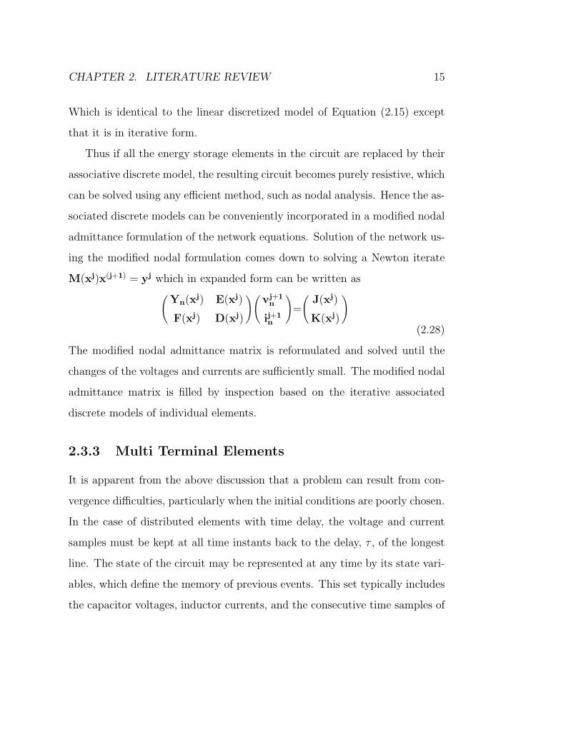
2.3.3 Multi Terminal Elements
It is apparent from the above discussion that a problem can result from con-
vergence difficulties, particularly when the initial conditions are poorly chosen.
In the case of distributed elements with time delay, the voltage and current
samples must be kept at all time instants back to the delay, τ , of the longest
line. The state of the circuit may be represented at any time by its state vari-
ables, which define the memory of previous events. This set typically includes
the capacitor voltages, inductor currents, and the consecutive time samples of
CHAPTER 2. LITERATURE REVIEW 16
the voltages and currents at the ports of the distributed elements. When the
initial conditions selected correspond to the physical turn on of the circuit,
SPICE enables the build up of transients to be readily examined. However,
when only the steady-state response is desired, this can be a burden, particu-
larly in the case when the differential equations representing the network are
stiff.
2.4 Iteration Methods
The two basic approaches to the iterative solution of nonlinear network equa-
tions are the fixed point algorithm, and the Newton algorithm. The notation
xj is used to indicate the jth iterative of x.
2.4.1 Fixed Point Method
In the fixed point algorithm a function F(x) needs to be developed with the
special property that xj+1 = F(x) is a better estimate of the function than xj
for the solution of f(x). The standard method of defining F(x) is
F(xj) = xj −K(xj)f (xj) (2.29)
where K(x) is a matrix function of x. The speed of convergence and whether
or not the iteration scheme is divergent depends heavily on the choice of K(x).
Then the iteration algorithm is
xj+1 = xj −K(xj)f (xj). (2.30)

CHAPTER 2. LITERATURE REVIEW 17
The iteration terminates when the difference between xj+1 and xj is less than
some prescribed acceptable error. This method requires that the error reduces
monotonically. Generally this occurs only for a narrow range of x near the
solution. If the fixed point iteration scheme is convergent, then it is linearly
convergent so that the error of consecutive iterations reduces linearly.
2.4.2 Newton Method
This is a variation of the fixed point method but with a good estimate of K(x).
Newtons method uses K(x) = [J(x)]−1 where J(x) is the Jacobian of f(x).
The iteration algorithm now becomes
xj+1 = xj − [J(xj)]−1f (xj) (2.31)
• The Newton method has good convergence properties and, if it is con-
vergent, has quadratic convergence. That is, if xj is close to the solution
then the error of consecutive iterations reduces quadratically.
• Higher order, e.g. cubic convergent schemes, can be used only with a
very narrow class of problems and estimates of x must be very close to
the solution for the schemes to converge.
• There can be a substantial cost, however, in storing, calculating and
inverting the Jacobian and so a Newton iteration followed by several
fixed point iterations are sometimes used (and termed the Shamanskii
method). This iteration scheme will be superlinearly (that is, more than
linearly but not quadratically) convergent.

CHAPTER 2. LITERATURE REVIEW 18
2.5 Summary
The use of state variables for transient analysis help represent the state of
the circuit at any time instant, which define the memory of previous events.
The set of nonlinear equations representing the elements of a circuit can be
discretized in time to form a set of linear algebraic equations. These equations
can be solved recursively at every time step, to find the nodal voltages of each
element and current flowing through the element.

19
Chapter 3
SPICE-Like Sparse Transient
Analysis
3.1 Nonlinear Equation Formulation
In this chapter the equations for the transient analysis are formulated with
the minimum number of unknowns starting from the nodal admittance matrix
of the linear part of the circuit. This approach has advantages that all the
flexibility of the modified nodal admittance matrix is maintained, and at the
same time has advantages given by the state variable approach.
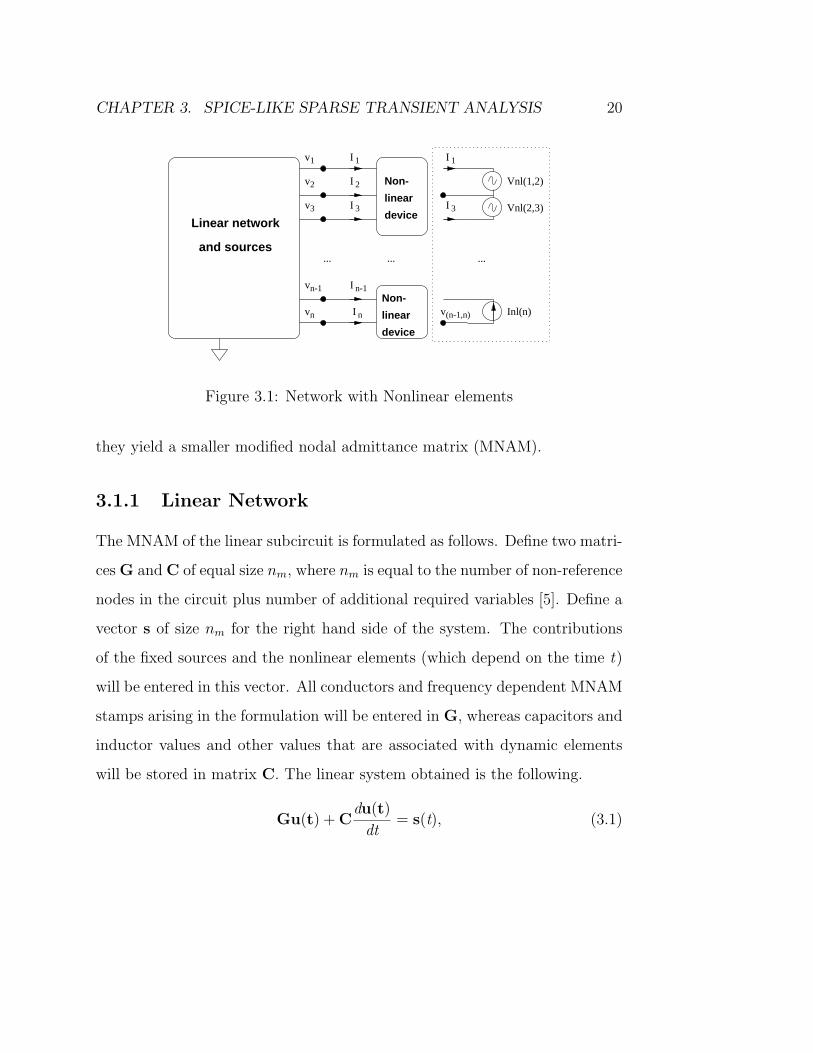
The formulation of the system equations begins with the partitioned net-
work of Figure 3.1 with the nonlinear elements replaced by variable voltage
or current sources [8]. For each nonlinear element one terminal is taken as
the reference and the element is replaced by a set of sources connected to the
reference terminal. Both voltage and current sources are valid replacements
for the nonlinear elements, but current sources are more convenient because
CHAPTER 3. SPICE-LIKE SPARSE TRANSIENT ANALYSIS 20
I 1
I 2
I 3
I n-1
nI
I 3
I 1
nv
...
Inl(n)
Vnl(1,2)
Vnl(2,3)
......
Linear network
and sources
Non-
linear
device
Non-
linear
device
n-1
3
2
1
v
v
v
v
v(n-1,n)
Figure 3.1: Network with Nonlinear elements
they yield a smaller modified nodal admittance matrix (MNAM).
3.1.1 Linear Network
The MNAM of the linear subcircuit is formulated as follows. Define two matri-
ces G and C of equal size nm, where nm is equal to the number of non-reference
nodes in the circuit plus number of additional required variables [5]. Define a
vector s of size nm for the right hand side of the system. The contributions
of the fixed sources and the nonlinear elements (which depend on the time t)
will be entered in this vector. All conductors and frequency dependent MNAM
stamps arising in the formulation will be entered in G, whereas capacitors and
inductor values and other values that are associated with dynamic elements
will be stored in matrix C. The linear system obtained is the following.
Gu(t) + Cdu(t)
dt= s(t), (3.1)

CHAPTER 3. SPICE-LIKE SPARSE TRANSIENT ANALYSIS 21
where u is the vector of the nodal voltages and required currents, and s is
composed of of an independent component sf and a component sv that depends
on the state variables, as in HB case [8].
s(t) = sf(t) + sv(t). (3.2)
The sf vector id due to the independent sources in the circuit. The sv vector is
the contribution of the currents injected into the linear circuit by the nonlinear
network.
3.1.2 Nonlinear Network
The concept of state variable used in this work is the one defined in Section
2.2.4. The Equations (2.9) and (2.10) are rewritten here for convenience:
vNL(t) = u[x(t),dx
dt, ...,
dmx
dtm,xD(t)] (3.3)
iNL(t) = w[x(t),dx
dt, ...,
dmx
dtm,xD(t)]. (3.4)
The error function of an arbitrary circuit is developed using connectivity infor-
mation (described by an incidence matrix and constitutive relations describing
the nonlinear elements). The incidence matrix, T, is built as follows. The
number of columns is nm, and the number of rows is equal to the number of
state variables, ns. In each row, enter “+1” in the column corresponding to
the positive terminal of the row nonlinear element port and “-1” in the column
corresponding to the negative terminal (the local reference of the port). Then,
each row of T has at most 2 nonzero elements and the number of nonzero
elements is at most 2ns.

CHAPTER 3. SPICE-LIKE SPARSE TRANSIENT ANALYSIS 22
The following equations are true for all t :
vL(t) = Tu(t) (3.5)
sv(t) = TT iNL(t) (3.6)
where vL(t) is the vector of the port voltages of the nonlinear elements calcu-
lated from the nodal voltages of the linear network.
3.1.3 Error Function Formulation
Now we have all the equations necessary to build a nonlinear error function
for the entire circuit. Combining Equations (3.1), (3.2) and (3.6), the general
equation for the linear network is obtained:
Gu(t) + Cdu(t)
dt= sf(t) + TT iNL(t). (3.7)
The reduced error function f(t) is defined as follows
f(t) = vL(t)− vNL(t) = 0. (3.8)
Replacing vL(t) from Equation (3.5)
f(t) = Tu(t)− vNL(t) = 0. (3.9)
Equations (3.3), (3.4), (3.7) and (3.8) confirm the generalized state variable
reduction formulation. The error function in Equation (3.8) only depends on
the state variables and the time derivatives:
f
[x(t),
dx
dt, ...,
dmx
dtm,xD(t)
]= 0. (3.10)

CHAPTER 3. SPICE-LIKE SPARSE TRANSIENT ANALYSIS 23
The dimension of the error function and the number of unknowns are equal
to ns, and this number is the minimum necessary to solve the equations of a
circuit without any loss of information. To reduce the error function formu-
lation the differential equations in an algebraic system of nonlinear equations
are converted to nonlinear algebraic systems using time marching integration
methods.
First Equations (3.3) and (3.4) are expressed using discretized time
vNL(xn) = u[xn,x′n, ...,x(m)n ,xD,n] (3.11)
iNL(xn) = w[xn,x′n, ...,x(m)n ,xD,n] (3.12)
where xn = x(tn), x′n = x′(tn), (xD,n)i = xi(tn - τi) and tn is the current time.
Discretization of Equation (3.7) yields
Gun + Cu′n = sf,n + TT iNL(xn). (3.13)
The time marching integration approximation used is given by,
x′n = axn + bn−1 (3.14)
where a is a constant and bn−1 depends on previous history of x. Applying
this equation to calculate the u′n vector gives,
u′n = aun + bn−1 (3.15)
where bn−1 has the same dimension as un. Replacing u′n in Equation (3.13),
Gun + C[aun + bn−1] = sf,n + TT iNL(xn). (3.16)
The size of the resulting algebraic system of nonlinear equation is ns.

CHAPTER 3. SPICE-LIKE SPARSE TRANSIENT ANALYSIS 24
3.1.4 Sparse Matrix Formulation
The solution to these nonlinear algebraic equations is transformed in the suc-
cessive solution of a sequence of linear circuits. This successive solution is
introduced by applying Equation (2.31) to calculate the iNL(xn) vector and
the vNL(xn)
iNL(x(j+1)n ) = iNL(xj
n) + Ji[x(j+1)n − xj
n] (3.17)
vNL(x(j+1)n ) = vNL(xj
n) + Jv[x(j+1)n − xj
n]. (3.18)
Replacing iNL(xn) in Equation (3.16) results in,
[G+Ca]u(j+1)n −TTJix
(j+1)n = [sf,n−Cabn−1]+TT [iNL(xj
n)−Jixjn]. (3.19)
Replacing vNL(xn) in Equation (3.9) results in,
Tu(j+1)n − vNL(xj
n)− Jv[x(j+1)n − xj
n] = 0. (3.20)
From Equation (3.19) and Equation (3.20) it can be seen that there are two
equations and two unknowns, u(j+1)n and x(j+1)
n . These equations can be solved
simultaneously. Since all the quantities in the two equations are vectors or
matrices, they can be put together giving a matrix equation of the form Ax =
B, where A is the coefficient matrix, x is the vector of unknown quantities
and B is the right hand side matrix.

CHAPTER 3. SPICE-LIKE SPARSE TRANSIENT ANALYSIS 25
Combining Equation (3.19) and Equation (3.20) results in,
[G + Ca] −[TTJi]
T −Jv
u(j+1)n
x(j+1)n
=
[sf,n −Cabn−1] +TT [iNL(xjn)− Jix
jn]
vNL(xjn) −Jvx
jn
. (3.21)
From the above Equation it can be seen that an equivalent linear circuit
is formed for every nonlinear element. The circuit is only equivalent to the
nonlinear element at the jth iteration because its element values (but not
its topology) change by discrete amounts at every iteration. This circuit is
repeatedly solved with updated element values till convergence is achieved.
In the above Equation the following observations can be made:
• Matrix G + Ca is sparse
• Matrix T is sparse
• Matrices Ji and Jv are sparse and block diagonal
Hence the matrix A thus formed is sparse. The above Equation can be solved
using LU factorization technique [9]. After solving Equation (3.21), the value
of the state variable vector and un is known, so finding vNL and iNL is straight-
forward.
The size of the resulting algebraic system of linear equations is (nm+ns)x(nm+ns).
G + Ca is constant as long as the time step h is constant. T is constant. The
right hand side vectors, Ji and Jv change at every Newton iteration and every

CHAPTER 3. SPICE-LIKE SPARSE TRANSIENT ANALYSIS 26
time step. Thus with every iteration the equivalent circuit of every element re-
mains same, as the topology remains the same, but the values of the elements
in the equivalent circuit change by discrete amounts at every iteration.
Note the matrices formed are sparse, so as the number of devices increase
nonlinear behavior of the elements is still handled the same way, unlike Har-
monic Balance where the nonlinear behavior is handled poorly as the number
of devices increase. As parameterized device models are used the DC bias
point for the circuit is calculated at the first time step with t = 0. These
voltages are set as the initial conditions for the transient analysis that follows.
3.1.5 Initial Operating Point
All circuits are biased at some dc operating point. This point should be
determined before the transient for better convergence. To determine the
dc operating point, all capacitors are opened, all inductors are shorted and
all controlled sources are set to zero. To realize this with the state variable
formulation, the derivatives of the state variables with respect to time are set
to zero.
3.2 Implementation in fREEDATM
Equation (3.21) resulted in a system of linear algebraic equations at every time
step and every Newton iteration. As the error function changes only slightly
from time step to time step, efficient matrix solving schemes can be used, as a
very good preconditioner is available from the previous time step. This system
CHAPTER 3. SPICE-LIKE SPARSE TRANSIENT ANALYSIS 27
Parse the inputnetlist
Create theMNAM
FormulateTransient equations
Calculate outputfrom state var.
Displayresults
Function andJacobian eval.SuperLU library
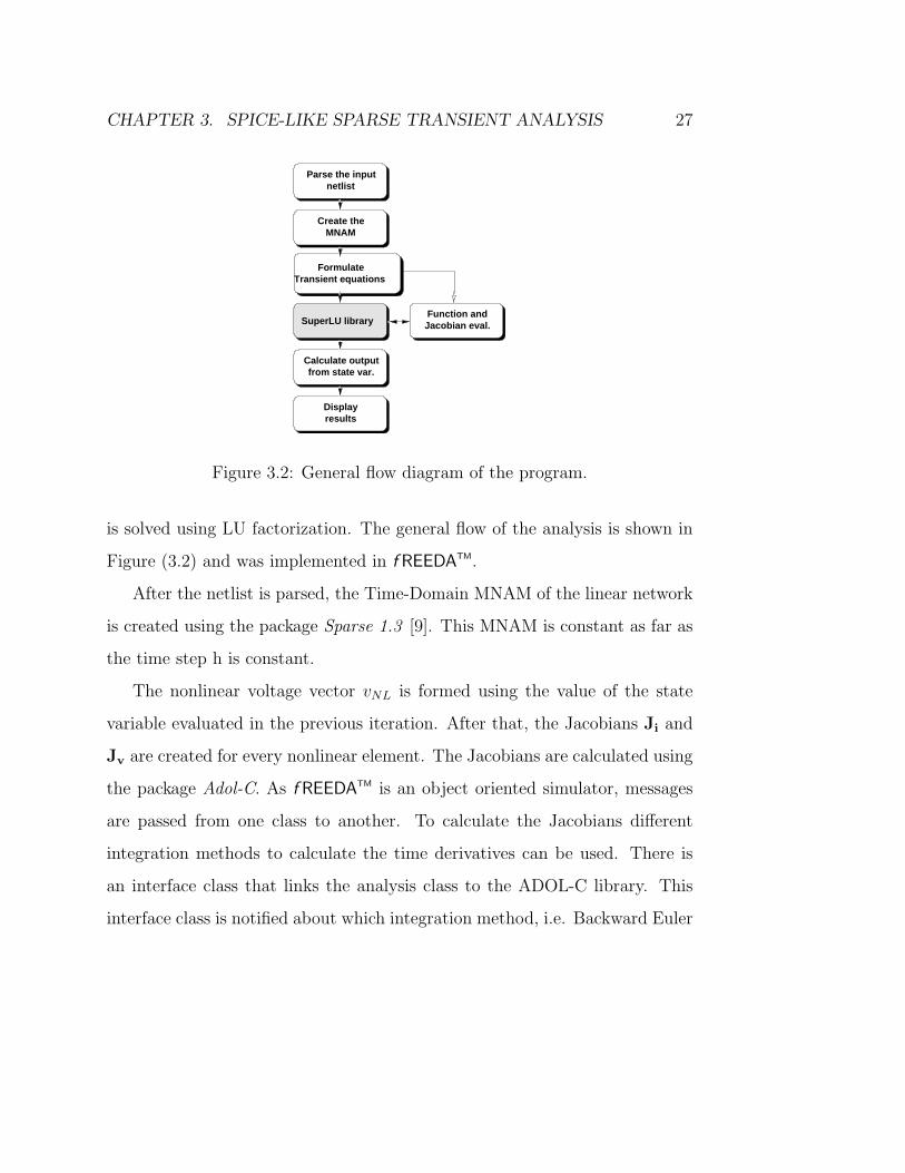
Figure 3.2: General flow diagram of the program.
is solved using LU factorization. The general flow of the analysis is shown in
Figure (3.2) and was implemented in f REEDATM.
After the netlist is parsed, the Time-Domain MNAM of the linear network
is created using the package Sparse 1.3 [9]. This MNAM is constant as far as
the time step h is constant.
The nonlinear voltage vector vNL is formed using the value of the state
variable evaluated in the previous iteration. After that, the Jacobians Ji and
Jv are created for every nonlinear element. The Jacobians are calculated using
the package Adol-C. As f REEDATM is an object oriented simulator, messages
are passed from one class to another. To calculate the Jacobians different
integration methods to calculate the time derivatives can be used. There is
an interface class that links the analysis class to the ADOL-C library. This
interface class is notified about which integration method, i.e. Backward Euler

CHAPTER 3. SPICE-LIKE SPARSE TRANSIENT ANALYSIS 28
or Trapezoidal method, has to be used to calculate the time derivatives.
With all these vectors the matrices in Equation (3.21) are formulated.
These matrices are solved using the package SuperLU. From the evaluated
value of state variables xn and nodal voltages un the nonlinear currents iNL
and nonlinear voltages vNL are calculated and stored to be used for the next
iteration. If the values of xn, un, iNL, vNL are within the tolerance limit, the
analysis advances in time to the next time step.
Once the equations are solved for all time steps, the requested currents and
voltages are saved in files.
The results are displayed using gnuplot. All the graphs requested in the
input netlist are plotted.
3.3 Support Libraries
A large number of software libraries are available (many of them freely) and
a few of them are used in f REEDATM.
3.3.1 Solution to Sparse Linear Systems
Sparse 1.3 [9] is a flexible package of subroutines written in C used to nu-
merically solve large sparse systems of linear equations. The package is able
to handle arbitrary real and complex square matrix equations. Besides being
able to solve linear systems, it is also able to quickly solve transposed systems,
find determinants, and estimate errors due to ill-conditioning in the system of
equations and instability in the computations. Sparse also provides a test pro-

CHAPTER 3. SPICE-LIKE SPARSE TRANSIENT ANALYSIS 29
gram that is able to read matrix equation from a file, solve it, and print useful
information (such as condition number of the matrix) about the equation and
its solution. Sparse was originally written for use in circuit simulators and is
well adapted to handling nodal- and modified-nodal admittance matrices.
SuperLU is used to solve the Equation (3.21) with LU factorization. It con-
tains a set of subroutines to numerically solve a sparse linear system Ax =
b. It uses Gaussian elimination with partial pivoting (GEPP). The columns
of A may be preordered before factorization; the preordering for sparsity is
completely separate from the factorization. SuperLU is implemented in ANSI
C. It provides support for both real and complex matrices, in both single and
double precision.
3.3.2 Vectors and Matrices
Most of the vector and matrix handling in f REEDATMuses MV++ [11]. This
is a small set of vector and simple matrix classes for numerical computing
written in C++. It is not intended as a general vector container class but
rather designed specifically for optimized numerical computations on RISC
and pipelined architectures which are used in most new computer architec-
tures. The various MV++ classes form the building blocks of larger user-level
libraries. The MV++ package includes interfaces to the computational ker-
nels of the Basic Linear Algebra Subprograms package (BLAS) which includes
scalar updates, vector sums, and dot products. The idea is to utilize vendor-
supplied, or optimized BLAS routines that are .ne-tuned for particular plat-
forms. The Matrix Template Library (MTL) is a high-performance generic

CHAPTER 3. SPICE-LIKE SPARSE TRANSIENT ANALYSIS 30
component library that provides comprehensive linear algebra functionality
for a wide variety of matrix formats. It is used in the above transient anal-
ysis. As with the STL, MTL uses a five-fold approach, consisting of generic
functions, containers, iterators, adaptors, and function objects, all developed
specifically for high performance numerical linear algebra. Within this frame-
work, MTL provides generic algorithms corresponding to the mathematical
operations that define linear algebra. Similarly, the containers, adaptors, and
iterators are used to represent and to manipulate matrices and vectors.
3.3.3 Automatic differentiation
The analytic Jacobian is calculated in the routine using Adol-C [10]. This
is a software package written in C and C++ and performs automatic differ-
entiation. The numerical values of the derivative vectors (required to fill the
Jacobians) are obtained free of truncation errors at a small multiple of the run
time required to evaluate the original function with little additional memory
required. The implementation of automatic differentiation in f REEDATM is
shown in Figure 3.3. The eval() method of the nonlinear element class is exe-
cuted at initialization time and so the operations to calculate the currents and
voltages of each element are recorded by Adol-C in a tape which is actually an
internal buffer. After that, each time that the values or the derivatives of the
nonlinear elements are required, an Adol-C function is called and the values
are calculated using the tapes. This implementation is efficient because the
taping process is done only once (this almost doubles the speed of the calcu-
lation compared to the case where the functions are taped each time they are
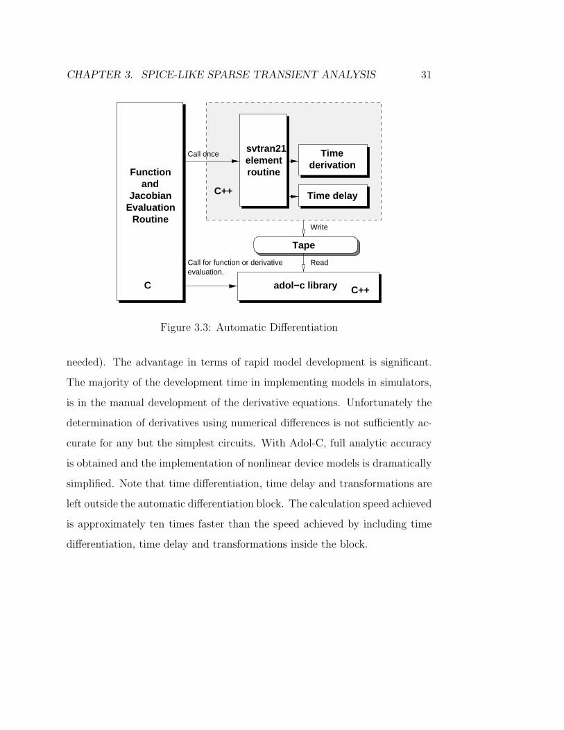
CHAPTER 3. SPICE-LIKE SPARSE TRANSIENT ANALYSIS 31
Time
routineelement derivation
svtran21
C
Call once
Call for function or derivativeevaluation.
Tape
adol−c library C++
Write
Read
Time delayC++
Functionand
JacobianEvaluation
Routine
Figure 3.3: Automatic Differentiation
needed). The advantage in terms of rapid model development is significant.
The majority of the development time in implementing models in simulators,
is in the manual development of the derivative equations. Unfortunately the
determination of derivatives using numerical differences is not sufficiently ac-
curate for any but the simplest circuits. With Adol-C, full analytic accuracy
is obtained and the implementation of nonlinear device models is dramatically
simplified. Note that time differentiation, time delay and transformations are
left outside the automatic differentiation block. The calculation speed achieved
is approximately ten times faster than the speed achieved by including time
differentiation, time delay and transformations inside the block.

CHAPTER 3. SPICE-LIKE SPARSE TRANSIENT ANALYSIS 32
3.4 Summary
The two aspects of the transient analysis of a nonlinear system are formula-
tion of the nonlinear equations and the method used to solve these nonlinear
equations. The nonlinear equations can be formulated as described in Section
3.1. This formulation keeps the flexibility of the modified nodal admittance
matrix, and has the advantages given by a state variable approach. The non-
linear equations thus formed can be solved as a sequence of linear equations
by applying Newton Raphson’s iteration method. The linear equations thus
formed can be represented in a sparse matrix, which can be solved using LU
factorization or any other efficient sparse matrix technique. The technique
discussed in this chapter can be efficiently applied to large systems.

33
Chapter 4
Results
4.1 Introduction
This chapter discusses the results of the analysis described in Chapter 3,
which was implemented in f REEDATM. Section 4.2 presents the results for
a Wide Band Amplifier. The speed and accuracy of the results obtained from
f REEDATM are compared to those obtained from HSPICE. Section 4.3 describes
the soliton line netlist used to validate the Sparse Matrix claim. The results
in this section describe how the sparsity of the matrix varies with the number
of elements used to model the line. A comparison of speed and accuracy of
the results obtained from f REEDATMand SPICE is made.
4.2 Wide Band Amplifier
The circuit used is from the MCNC benchmark suite established around 1990.
The amplifier circuit consists of 11 Gummel-Poon Bipolar Transistors, see

CHAPTER 4. RESULTS 34
Sparse Transient Time Marching Transient SPICE(s)in f REEDATM(s) in f REEDATM(s)
71 76 22
Table 4.1: Comparison of simulation times for the wide band amplifier.
Figure 4.1. This circuit was simulated to test the accuracy and speed of
the new transient analysis implemented in f REEDATM. The amplifier circuit
was simulated in f REEDATMand SPICE. The output waveforms and voltage
amplitudes were found to match, thus validating the accuracy of the new
transient analysis. The netlist for this circuit is provided in Appendix B.
This circuit was simulated for 50 ns with a fixed time step of 10 ps on a
Pentium III Xeon clocked at 500 MHz. Figures 4.2 and 4.3 show the voltages at
the nodes out16 and out17 of the amplifier, shown in Figure 4.1. In Figure 4.2
waveform (a) and (b) are the output voltages at the terminals out17 and out16
respectively. From the two figures it can be seen that the output waveforms
are in excellent agreement. During the simulation, a matrix of size 54 × 54
was formed and 33 state variables were used. 7.784% of the elements in the
matrix formed were non-zero, making the matrix approximately 92% sparse.
The simulation was completed in 71s.
From Table 4.1 it can also be seen that a time marching transient analysis
with state variables [1] is slower than the new analysis, but only marginally.
This is because the time marching transient analysis factorizes the Jacobian,
wherein maximum time is spent in inverting the Jacobian Matrix. The factor-
ization of the Jacobian is expensive for circuits with large number of nonlinear

CHAPTER 4. RESULTS 35
Figure 4.1: Wideband amplifier, from the MCNC benchmark suite with 11Gummel-Poon Bipolar Transistors.

CHAPTER 4. RESULTS 36
0
2
4
6
8
10
12
0 5 10 15 20 25 30 35 40 45 50
Vol
tage
(V
)
Time (ns)
(a)
(b)
Figure 4.2: Output voltages at terminals out17, curve (a), and out16, curve(b), of the wideband amplifier simulated in f REEDATM.

CHAPTER 4. RESULTS 37
time
0.0 5.0 10.0 15.0 20.0 25.0 30.0 35.0 40.0 45.0 50.0
nS
2.0
3.0
4.0
5.0
6.0
7.0
8.0
9.0
10.0
11.0
(a)
(b)
Figure 4.3: Output voltages at terminals out17, curve (a), and out16, curve(b), of the wideband amplifier simulated in SPICE.

CHAPTER 4. RESULTS 38
devices. As the new analysis does not factorize the Jacobian, it is faster.
The improvement in speed will be significant for circuits with large number of
nonlinear elements (more than a few hundred).
This circuit was simulated in SPICE with a maximum time step of 10ps.
From Table 4.1 it can be seen that, the new analysis is slower than SPICE. This
can be explained as follows. Traditional circuit simulators like SPICE, must
perform the decomposition of a sparse matrix (size nm×nm) at each iteration
of the method to solve the nonlinear equations [3]. Here m corresponds to
the number of terminals with the voltage at each terminal being an unknown.
But as f REEDATMuses the idea of state variables to model its elements, the
new analysis has to decompose a sparse matrix of size (nm + ns)× (nm + ns),
where ns is the number of state variables used. Therefore size of the sparse
matrix is larger because the number of unknowns is more. The state variable
approach gives more accurate models and makes model development easier.
Therefore speed is traded off here, for accuracy and ease of development of
models. f REEDATM is an object oriented simulator [13], and uses many support
libraries. The object oriented approach speeds up the process of developing
models i.e. writing code for the models. During simulation messages are passed
and data is copied from one class to another. This is a little expensive than
procedural programming. The most significant impact on speed is because the
new analysis does not use variable time step control. Thus it cannot use long
time steps at the beginning of the simulation. A state variable based time
step control [12] can be easily implemented for the new analysis. This new
time step algorithm uses a predictor-corrector technique, with high accuracy

CHAPTER 4. RESULTS 39
Figure 4.4: 47 diode soliton line.
of results.
4.3 Soliton Line
4.3.1 Circuit
A nonlinear transmission line is regarded by many in the field as an extreme
test of the performance of transient and steady-state simulators. Nonlinear
transmission lines (NLTLs) find applications in a variety of high speed, wide
bandwidth systems including picosecond resolution sampling circuits, laser
and switching diode drivers, test waveform generators, and mm-wave sources.
They have three fundamental characteristics: nonlinearity, dispersion and dis-
sipation. The NLTL considered here consists of coplanar waveguides (CPWs)
periodically loaded with reverse biased Schottky diodes. A diode-based NLTL
used for pulse generation is an extremely nonlinear circuits and is used to test
the robustness of circuit simulators. The NLTL considered here was designed
with a balance between the nonlinearity of the loaded nonlinear elements and
the dispersion of the periodic structure which results in the formation of a
stable soliton. The nonlinearity of NLTLs is principally due to the voltage de-
pendent capacitance of the diodes and the dissipation is due to the conductor
losses in the CPWs.

CHAPTER 4. RESULTS 40
-18
-16
-14
-12
-10
-8
-6
-4
-2
0
450 460 470 480 490 500 510
Dio
de 4
7 V
olta
ge
Time (ps)
Transim TrapezoidalTransim B. Euler
Spice
Figure 4.5: Comparison of the voltage at the last diode of the soliton line.
The NLTL was modelled using generic transmission lines with frequency
dependent loss and Schottky diodes. Skin effect was taken into account in the
modeling of the transmission lines. The NLTL model is shown in Figure 4.4
and is excited by a 9 GHz sinusoid. The NLTL was designed for a 24 GHz
initial Bragg frequency, 225 GHz final Bragg frequency, 0.952097 tapering rule,
and 120 ps total compression. It contains 48 sections of CPW transmission
lines and 47 diodes. The drive is a 27 dBm sine wave at −3 V dc bias. The
netlist for this circuit is provided in Appendix C.

CHAPTER 4. RESULTS 41
4.3.2 Results
This circuit was simulated with f REEDATMfor 0.55 ns. Figure 4.5 compares
the voltage at the last diode obtained using Backward Euler and Trapezoidal
integration method and the SPICE simulation. The fixed time step used was
0.01 ps for BE and 0.1 ps for Trapezoidal. The waveforms are in excellent
agreement. Note that even though a small time step is used, the numerical
damping introduced by BE method attenuates the small oscillations in the
waveform.
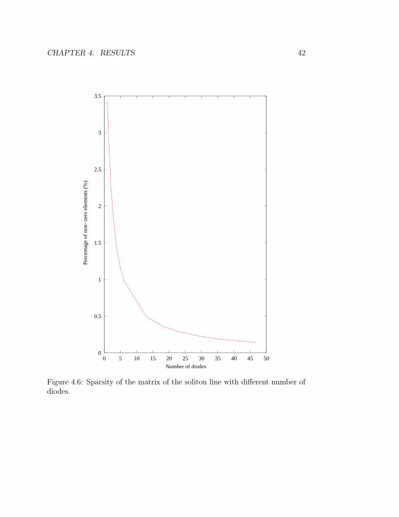
From Figure 4.6 it can be seen that as the number of nonlinear elements
in the circuit, here Schottky diodes, increases the sparsity of the matrix in-
creases ( i.e. the percentage of non-zero elements decreases). This is because,
the number of equations to be solved increases with the number of elements,
making the matrix larger and sparser. The efficiency of the LU factorization
technique improves with size and sparsity of the matrix.
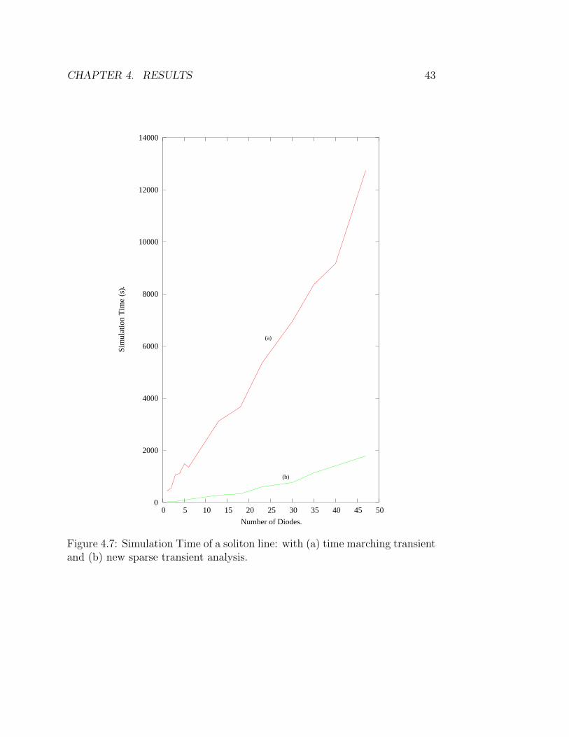
In Figure 4.7 a comparison between the simulation time of a time marching
transient analysis and the new analysis is made. The new analysis considers
every element to be a nonlinear element. To make a fair comparison between
the two analysis, every element in the time marching transient analysis is con-
sidered as a nonlinear element, and the required simulation time is found. The
figure shows that the new analysis is faster. The new analysis is approximately
7.13 times faster than the time marching transient analysis.
From Table 4.2 it can be seen that SPICE is about 1.35 times faster than
the new analysis. This is because SPICE does not model its devices with state
variables, and hence and has relatively less number of unknowns than those in
CHAPTER 4. RESULTS 42
0
0.5
1
1.5
2
2.5
3
3.5
0 5 10 15 20 25 30 35 40 45 50
Perc
enta
ge o
f no
n−ze
ro e
lem
ents
(%
)
Number of diodes
Figure 4.6: Sparsity of the matrix of the soliton line with different number ofdiodes.
CHAPTER 4. RESULTS 43
0
2000
4000
6000
8000
10000
12000
14000
0 5 10 15 20 25 30 35 40 45 50
Sim
ulat
ion
Tim
e (s
).
Number of Diodes.
(a)
(b)
Figure 4.7: Simulation Time of a soliton line: with (a) time marching transientand (b) new sparse transient analysis.

CHAPTER 4. RESULTS 44
Sparse Transient SPICE(s)in f REEDATM(s)
1795 1322
Table 4.2: Comparison of simulation times of a 47 diode soliton line.
f REEDATM. Therefore the size of the matrix to be solved in SPICE is smaller
than that in f REEDATM.
Note that the soliton line with 47 diodes, has 47 inductors and 48 trans-
mission lines. The transmission lines are modelled in f REEDATMas a set RLC
elements, i.e. a set of linear elements. Thus the total number of linear el-
ements in the circuit is 95, which is greater than two times the number of
nonlinear elements. This makes the incidence matrix (T) in Equation (3.21)
large, thus making the multiplication (TT × Ji) expensive for a circuit with a
large number of linear elements. Whereas, in the previous section, the Wide-
band Amplifier circuit has 12 resistors and 11 transistors, i.e. the number
of nonlinear elements is almost equal to the number of linear elements. This
makes the incidence matrix (T) smaller in size, effectively improving the speed
of the simulation. Thus from the above result it can be concluded that the
new analysis is best suited for circuits with large number of nonlinear elements
so ns À nm.
CHAPTER 4. RESULTS 45
4.4 Summary
The use of sparse matrix techniques improves the efficiency of a state variable
based transient analysis. The sparsity of the matrices increases with the size
of the circuits. The reduction in simulation time is significant in large circuits,
with large number of nonlinear elements. The comparison of output waveforms
of the wideband amplifier and soliton line with different transient analysis
techniques shows that, high accuracy is achieved with the new analysis.

46
Chapter 5
Conclusions and Future
Research
5.1 Conclusions
This analysis was successfully developed in f REEDATMand was found to be
robust and flexible. A sparse matrix approach is generally used in simulators
for the transient analysis of circuits. The challenge here was using universal
device modeling where the code defining the model of an element needs to be
written once and used in many different types of analyses.
The following conclusions are made:
• The equation formulation eliminates the need to factorize the Jacobian.
• Time and Newton discretization of the nonlinear elements results in an
algebraic system of linear equations.
• The sparsity of the matrix increases with circuit size, improving efficiency

CHAPTER 5. CONCLUSIONS AND FUTURE RESEARCH 47
of the analysis.
• The analysis is best suited for circuits with large number of nonlinear
elements so that the number of state variables (ns) is much greater than
the number of terminals (nm).
5.2 Future Research
There are many improvements that can be made to the current implemen-
tation of the sparse transient analysis in f REEDATM.
The most important of them is use of efficient memory management to
manage the large sparse matrix formed. This large matrix is formulated and
factorized at every iteration. As for every iteration only some part of the ma-
trix changes, an efficient memory management technique, which uses pointer
to pointer dereferencing, would avoid reformulating the matrix for every iter-
ation. This would make the analysis faster.
As mentioned above, values of only some elements of the matrix change
with every iteration and the non zero structure of the matrix does not change at
every iteration. Some techniques, like chord iterations, take advantage of this.
These techniques, decompose the matrix once and update the decomposed
matrix at every iteration. This technique along with an efficient memory
management scheme will speed up the simulation significantly.
Also, currently the sparse transient analysis does not use time step control.
The use of variable time step, will allow the analysis to use long time steps at
the beginning of the simulation. Hence it would improve accuracy and speed

CHAPTER 5. CONCLUSIONS AND FUTURE RESEARCH 48
of the analysis.

49
Appendix A
Computer Code
Computer Code
This section contains the various functions in the C++ class of the sparse
transient analysis.
/***************************************************************************
*
* Contains the state variable based sparse transient analysis
*
****************************************************************************/
/*The include files*/
#include "SVTran21.h" #include "TimeMNAM.h" #include
"TimeDomainSV.h" #include "NLSInterface.h" #include "Euler.h"
#include "Trapezoidal.h" #include "iostream.h" #include
MV_P"/mvblasd.h"
extern int superLU_print_enable ; extern "C" { #include
"../inout/ftvec.h" #include "../inout/report.h"
}

APPENDIX A. COMPUTER CODE 50
/*This routine develops the incidence matrix T.*/
void buildTIncidence(ElemFlag mask, Circuit*& my_circuit,
IntMatrix& T, ElementVector& elem_vec,
int& n_states, int& max_n_states);
// Element information
ItemInfo SVTran21::ainfo = {
"SVTran2",
"State-Variable-Based Time-Marching Transient Analysis with Newton Iterations.",
"Sonali R. Luniya",
DEFAULT_ADDRESS
};
/*Parameter information about the analysis.*/
ParmInfo SVTran21::pinfo[] = {
{"tstop", "Stop time (s)", TR_DOUBLE, true},
{"tstep", "Time step (s)", TR_DOUBLE, true},
{"nst", "No save time (s)", TR_DOUBLE, false},
{"deriv", "Approximate derivatives or use automatic diff.", TR_INT, false},
{"msv", "Use Msv flag", TR_BOOLEAN, false},
{"im", "Integration method", TR_INT, false},
{"savenode", "Save node voltages", TR_BOOLEAN, false},
{"permc_spec", "Permutation ordering to factor Msv (0, 1 or 2)",
TR_INT, false},
{"out_steps", "Number of steps skipped for output simulation progress",
TR_INT, false},
{"gcomp", "Compensation network conductance (S)", TR_DOUBLE, false}
};
/*Constructor to set the default values of the analysis
parameters.*/

APPENDIX A. COMPUTER CODE 51
SVTran21::SVTran21() : Analysis(&ainfo, pinfo,n_par), ls_size(0),
superLU(false)
{
// Parameter stuff
paramvalue[0] = &(tf);
paramvalue[1] = &(h);
paramvalue[2] = &(nst = zero);
paramvalue[3] = &(deriv = 0);
paramvalue[4] = &(use_msv = true);
paramvalue[5] = &(int_method = 1);
paramvalue[6] = &(savenode = true);
paramvalue[7] = &(permc_spec = 2);
paramvalue[8] = &(out_steps = 200);
paramvalue[9] = &(gcomp = 0);
}
/*The main analysis routine.*/
void SVTran21::run(Circuit* cir) {
/* Build time domain MNAM */
TimeMNAM mnam(cir, mnam_mask);
/*Build T matrix and nonlinear element vector.*/
buildTIncidence(mask, cir, T, elem_vec, n_states, max_n_states);
/*Setup simulation variables (use circular vectors).*/
SparseMatrix *M ;
/*Set the type of integration method to be used Trapezoidal or
Backward Euler.*/
/*Copy the MNAM to sparsematrix M1.*/
l_im->buildMd(M1, h);

APPENDIX A. COMPUTER CODE 52
M = new SparseMatrix(ls_size+n_states,ls_size+n_states);
/*Formulate the incidence matrix from the condensed incidence
matrix.*/
for(int k =0 ; k < n_states ; k++ )
{
if (T(0,k))
{
tmpidx =T(0,k) -1 ;
myT[k][tmpidx] = 1;
}
if(T(1,k) )
{
tmpidx =T(1,k) -1 ;
myT[k][tmpidx] =-1;
}
}
/*Add the MNAM to Sparse matrix M. The sparse matrix stores only
the nonzero values in vector elem_val[] and their row and colummn
indices in vectors row_index[] and col_pointer[] respectively.*/
/*Add incidence matrix T to Sparse Matrix.*/
/*Number of time steps.*/
n_tsteps = int(tf / h + 1);
/*Create a Time domain interface. This class has data structures
that store the values of the state variables, nodal voltages and
currents at every time step.*/
tdsv = new TimeDomainSV(&(cX->getCurrent()[0]),
&(cVnl->getCurrent()[0]),
&(cInl->getCurrent()[0]),max_n_states);
APPENDIX A. COMPUTER CODE 53
/*Start the simulation from time =0.*/
for ( nt=0; nt < n_tsteps; nt++)
{
/*Build the vector of independent sources.*/
l_im->buildSf(sf, ctime);
/*Start Newton Iterations.*/ do
{
/*For every element formulate the Jacobians.*/
elem_vec[k]->svTran(tdsv);
elem_vec[k]->deriv_svTran(tdsv); // Call element evaluation
/*Multiply the Jacobian by T’ and add to the Sparse Matrix M.*/
/*Add or subtract the value of the Jacobian according to a +1 or a
-1 in the Jacobian.*/
elem_val[i]+=Ji_elem(j,m);
elem_val[i]= -Ji_elem(j,m);
/*Add Ju to the sparse matrix M.*/ /*Multiply Ju by cX i.e the
state variable vector and add it to the RHS vector.*/
elem_val[scount]= -Ju_elem(i,m);
row_index[scount]=ls_size+i+ibase;
scount++;
rhs_Jv_X[i+ibase]+=Ju_elem(i,m)*cX->getCurrent()[m+ibase];
/*Multiply T’JiXi.*/
multiply(rhs_temp , xtmp1, tmp_vec1);
/*Multiply T’*Inl.*/ /*Prepare the RHS vector.*/ /*LU factorize
the matrix.*/

APPENDIX A. COMPUTER CODE 54
superLUFactor(M,ssv);
/*Check for error between the two Newton iterations.*/
if(error > 0.001)
{ continue }
/*Update the values of the nodal voltages and currents.*/
updateVInl(&(ssv[0]));
if(iteration >= 40)
{
sprintf(msg , "Newton Raphson didn’t converge |%f \t|",error);
report(MESSAGE, msg);
}
} while (error > 0.001 && iteration <40) /*End Newton
iterations.*/
/*Update previous derivatives in integration method (if
required).*/
/*Store state variables for next time step.*/
cX->getCurrent()[i] =ssv[ls_size+i];
/*Write outputs .*/
doOutput();
}
void SVTran21::superLUFactor(SparseMatrix*& M, DenseVector& ssv) {
/*Create the matrix A to be factorized.*/
/*Create the RHS vector B.*/ /*Create resultant matrix X.*/ /*get
the Permutations.*/
get_perm_c(permc_spec, &A, perm_c);

APPENDIX A. COMPUTER CODE 55
/*Factorize and solve the matrix. The factors are stored in L and
U and the result in stored in ssv[].*/
dgssvx(&fact, &trans, &refact, &A, ftp, perm_c, perm_r, etree, &equed, r, c,
&L, &U, work, lwork, &B, &X, &recip_pivot_growth, &rcond,
&ferr, &berr, &mem_usage, &info);
}
void SVTran21::freeSuperLU() { /*Delete the storage required for
the LU factorization.*/ }
/*Simple matrix multiplication.*/
void SVTran21::multiply(DoubleMatrix& a , ExtVector& b ,
DoubleVector& c) {
}
void SVTran21::updateVInl(double* x_p) { /*Copy new value of U
into the Circ Vector.*/
for(int j=0 ; j< ls_size; j++)
cU->getCurrent()[j] = x_p[j];
/*Copy new value of X into Circ Vector.*/
for (int j=0; j < n_states; j++)
cX->getCurrent()[j] = x_p[ls_size+j];
}
/*Write the data to the output vectors.*/
void SVTran21::doOutput() { /* First check if the result
matrices contain any data.*/
/*Create temporary storage.*/
/*Now fill currents and port
voltages of time domain devices.*/ /*For every element do the
following.*/

APPENDIX A. COMPUTER CODE 56
/*For the current, decompensate while copying.*/
for (int tindex=0; tindex < out_size; tindex++) {
tmp_x[tindex] = cX->getPrevious(out_size - tindex)[j+i];
tmp_i[tindex] = cInl->getPrevious(out_size - tindex)[j+i];
tmp_u[tindex] = cVnl->getPrevious(out_size - tindex)[j+i];
}
elem_vec[k]->getElemData()->setRealX(j, tmp_i);
elem_vec[k]->getElemData()->setRealI(j, tmp_i);
elem_vec[k]->getElemData()->setRealU(j, tmp_u);
}
if (savenode) {
/* For each terminal, assign voltage vector.*/
/* Set the terminal vector.*/
term->getTermData()->setRealV(tmp_u);
}
}

57
Appendix B
Wideband Amplifier Netlist
Wideband Amplifier Netlist
This section contains the netlist for the wideband amplifier, discussed in
section 4.2.
*rca netlist
* Wide Band Amp.
r:rs1 30 1 r=1k r:rs2 31 0 r=1k r:r1 5 3 r=4.8k r:r2 6 3 r=4.8k
r:r3 9 3 r=811 r:r4 8 3 r=2.17k r:r5 8 0 r=820 r:r6 2 14 r=1.32k
r:r7 2 12 r=4.5k r:r8 2 15 r=1.32k r:r9 16 0 r=5.25k r:r10 17 0
r=5.25k bjtnpn:q1 2 30 5 0 model="qnl" bjtnpn:q2 2 31 6 0
model="qnl" bjtnpn:q3 10 5 7 0 model="qnl" bjtnpn:q4 11 6 7 0
model="qnl" bjtnpn:q5 14 12 10 0 model="qnl" bjtnpn:q6 15 12 11 0
model="qnl" bjtnpn:q7 12 12 13 0 model="qnl" bjtnpn:q8 13 13 0 0
model="qnl" bjtnpn:q9 7 8 9 0 model="qnl" bjtnpn:q10 2 15 16 0
model="qnl" bjtnpn:q11 2 14 17 0 model="qnl"
*****************************************bjt model
statement********************** .model qnl bjtnpn(bf=80 rb=100
tf=.3ns tr=6ns rb=100 cje=3pf cjc=2pf vaf=50)
************************************************************************************
APPENDIX B. WIDEBAND AMPLIFIER NETLIST 58
vsource:vin 1 0 vdc=0. vac=.1 f=50e6 phase = -90 delay = 1ns
vsource:vcc 2 0 vdc=15 tr=10ps vsource:vee 3 0 vdc=-15 tr=10ps
*******************************************Transient
Analysis********************** .tran21 tstop=50ns tstep=10ps im=0
out_steps=500
************************************************************************************
.out plot term 1 vt in "out.vt1" .out plot term 16 vt in
"out.vt16" .out plot term 17 vt in "out.vt17"
.end

59
Appendix C
Soliton Line Netlist
Soliton Line Netlist
This section contains the netlist for the soliton line discussed in section 4.3.
Figures 4.6 and 4.7 show how the sparsity of the matrix and the simulation
time vary with the number of diodes, respectively. To get these results the
netlist given below was modified, such that the number of L-sections in the
circuit is equal to the number of diodes. For example, for a soliton line with 1
L-section, the netlist included , diode d1, transmission line t1 and the inductor
i1. Off course, the source (rs) and load (rl) resistors and the transmission line
(t0) in series with the source resistor were always included. Similarly for higher
number of diodes the necessary elements were included. The tapering rule was
kept constant at 0.952097.
*Soliton using good parameters
* Transim file for NLTL with 24.00 GHz initial Bragg frequency,

APPENDIX C. SOLITON LINE NETLIST 60
* 225.00 GHz final Bragg frequency and 0.952097 tapering rule,
* and 120.00 ps total compression.
.options freq=9.GHz nonlin=4 rtol=1e-4 ftol=rtol maxit=100
.tran21 tstop=.55e-9 tstep=.1ps msv=1 im=1 savenode=0
*
* For 27dBm input use vac = 14V
* vsource:1 201 0 vac = 14. vdc = -6. f = freq phase=90 tr=.1e-9
r:rs 201 202 r=50.
*
* Diode parameters
*
* From thesis: js=2.24e-12, alfa=21.13
*
* From Libra netlist: js=51e-15, alfa=default
* .model carlos diode ( js=2.24e-12 alfa=21.13 e=10
ct0=1.32767e-15 r0=171.9 + fi=1.27517 gama=0.810205 jb=1.e-5
vb=-16. )
*
* Transmission line parameters
* .model c_line tlinp4 ( z0mag=75.00 k=7 fscale=10.e9 alpha = 59.9
+ nsect = 20 fopt=10e9)
*
* Diodes
* diode:d1 101 0 model = "carlos" area=271.64 diode:d2 102 0 model
= "carlos" area=258.63 diode:d3 103 0 model = "carlos"
area=246.24 diode:d4 104 0 model = "carlos" area=234.45 diode:d5
105 0 model = "carlos" area=223.21 diode:d6 106 0 model =
"carlos" area=212.52 diode:d7 107 0 model = "carlos" area=202.34
diode:d8 108 0 model = "carlos" area=192.65 diode:d9 109 0 model
= "carlos" area=183.42 diode:d10 110 0 model = "carlos"

APPENDIX C. SOLITON LINE NETLIST 61
area=174.63 diode:d11 111 0 model = "carlos" area=166.27
diode:d12 112 0 model = "carlos" area=158.3 diode:d13 113 0
model = "carlos" area=150.72 diode:d14 114 0 model = "carlos"
area=143.5 diode:d15 115 0 model = "carlos" area=136.63 diode:d16
116 0 model = "carlos" area=130.08 diode:d17 117 0 model =
"carlos" area=123.85 diode:d18 118 0 model = "carlos" area=117.92
diode:d19 119 0 model = "carlos" area=112.27 diode:d20 120 0
model = "carlos" area=106.89 diode:d21 121 0 model = "carlos"
area=101.77 diode:d22 122 0 model = "carlos" area=96.89 diode:d23
123 0 model = "carlos" area=92.25 diode:d24 124 0 model =
"carlos" area=87.83 diode:d25 125 0 model = "carlos" area=83.63
diode:d26 126 0 model = "carlos" area=79.62 diode:d27 127 0
model = "carlos" area=75.81 diode:d28 128 0 model = "carlos"
area=72.18 diode:d29 129 0 model = "carlos" area=68.72 diode:d30
130 0 model = "carlos" area=65.43 diode:d31 131 0 model =
"carlos" area=62.29 diode:d32 132 0 model = "carlos" area=59.31
diode:d33 133 0 model = "carlos" area=56.47 diode:d34 134 0
model = "carlos" area=53.76 diode:d35 135 0 model = "carlos"
area=51.19 diode:d36 136 0 model = "carlos" area=48.73 diode:d37
137 0 model = "carlos" area=46.4 diode:d38 138 0 model =
"carlos" area=44.18 diode:d39 139 0 model = "carlos" area=42.06
diode:d40 140 0 model = "carlos" area=40.05 diode:d41 141 0
model = "carlos" area=38.13 diode:d42 142 0 model = "carlos"
area=36.3 diode:d43 143 0 model = "carlos" area=34.56 diode:d44
144 0 model = "carlos" area=32.91 diode:d45 145 0 model =
"carlos" area=31.33 diode:d46 146 0 model = "carlos" area=29.83
diode:d47 147 0 model = "carlos" area=28.4
*
* Parasitic inductors
* l:i1 1 101 l=21.8pH l:i2 2 102 l=21.8pH l:i3 3 103 l=21.8pH
l:i4 4 104 l=21.8pH l:i5 5 105 l=21.8pH l:i6 6 106 l=21.8pH
l:i7 7 107 l=21.8pH l:i8 8 108 l=21.8pH l:i9 9 109 l=21.8pH
l:i10 10 110 l=21.8pH l:i11 11 111 l=21.8pH l:i12 12 112 l=21.8pH
l:i13 13 113 l=21.8pH l:i14 14 114 l=21.8pH l:i15 15 115 l=21.8pH
l:i16 16 116 l=21.8pH l:i17 17 117 l=21.8pH l:i18 18 118 l=21.8pH

APPENDIX C. SOLITON LINE NETLIST 62
l:i19 19 119 l=21.8pH l:i20 20 120 l=21.8pH l:i21 21 121 l=21.8pH
l:i22 22 122 l=21.8pH l:i23 23 123 l=21.8pH l:i24 24 124 l=21.8pH
l:i25 25 125 l=21.8pH l:i26 26 126 l=21.8pH l:i27 27 127 l=21.8pH
l:i28 28 128 l=21.8pH l:i29 29 129 l=21.8pH l:i30 30 130 l=21.8pH
l:i31 31 131 l=21.8pH l:i32 32 132 l=21.8pH l:i33 33 133 l=21.8pH
l:i34 34 134 l=21.8pH l:i35 35 135 l=21.8pH l:i36 36 136 l=21.8pH
l:i37 37 137 l=21.8pH l:i38 38 138 l=21.8pH l:i39 39 139 l=21.8pH
l:i40 40 140 l=21.8pH l:i41 41 141 l=21.8pH l:i42 42 142 l=21.8pH
l:i43 43 143 l=21.8pH l:i44 44 144 l=21.8pH l:i45 45 145 l=21.8pH
l:i46 46 146 l=21.8pH l:i47 47 147 l=21.8pH
*
* Transmission lines
* tlinp4:t0 202 0 1 0 model = "c_line" length=501.29u tlinp4:t1 1
0 2 0 model = "c_line" length=978.57u tlinp4:t2 2 0 3 0 model =
"c_line" length=931.69u tlinp4:t3 3 0 4 0 model = "c_line"
length=887.06u tlinp4:t4 4 0 5 0 model = "c_line" length=844.57u
tlinp4:t5 5 0 6 0 model = "c_line" length=804.11u tlinp4:t6 6 0
7 0 model = "c_line" length=765.59u tlinp4:t7 7 0 8 0 model =
"c_line" length=728.92u tlinp4:t8 8 0 9 0 model = "c_line"
length=694.00u tlinp4:t9 9 0 10 0 model = "c_line" length=660.75u
tlinp4:t10 10 0 11 0 model = "c_line" length=629.10u tlinp4:t11
11 0 12 0 model = "c_line" length=598.97u tlinp4:t12 12 0 13 0
model = "c_line" length=570.27u tlinp4:t13 13 0 14 0 model =
"c_line" length=542.96u tlinp4:t14 14 0 15 0 model = "c_line"
length=516.95u tlinp4:t15 15 0 16 0 model = "c_line"
length=492.18u tlinp4:t16 16 0 17 0 model = "c_line"
length=468.61u tlinp4:t17 17 0 18 0 model = "c_line"
length=446.16u tlinp4:t18 18 0 19 0 model = "c_line"
length=424.79u tlinp4:t19 19 0 20 0 model = "c_line"
length=404.44u tlinp4:t20 20 0 21 0 model = "c_line"
length=385.06u tlinp4:t21 21 0 22 0 model = "c_line"
length=366.62u tlinp4:t22 22 0 23 0 model = "c_line"
length=349.05u tlinp4:t23 23 0 24 0 model = "c_line"
length=332.33u tlinp4:t24 24 0 25 0 model = "c_line"
length=316.41u tlinp4:t25 25 0 26 0 model = "c_line"

APPENDIX C. SOLITON LINE NETLIST 63
length=301.26u tlinp4:t26 26 0 27 0 model = "c_line"
length=286.83u tlinp4:t27 27 0 28 0 model = "c_line"
length=273.09u tlinp4:t28 28 0 29 0 model = "c_line"
length=260.00u tlinp4:t29 29 0 30 0 model = "c_line"
length=247.55u tlinp4:t30 30 0 31 0 model = "c_line"
length=235.69u tlinp4:t31 31 0 32 0 model = "c_line"
length=224.40u tlinp4:t32 32 0 33 0 model = "c_line"
length=213.65u tlinp4:t33 33 0 34 0 model = "c_line"
length=203.42u tlinp4:t34 34 0 35 0 model = "c_line"
length=193.67u tlinp4:t35 35 0 36 0 model = "c_line"
length=184.39u tlinp4:t36 36 0 37 0 model = "c_line"
length=175.56u tlinp4:t37 37 0 38 0 model = "c_line"
length=167.15u tlinp4:t38 38 0 39 0 model = "c_line"
length=159.14u tlinp4:t39 39 0 40 0 model = "c_line"
length=151.52u tlinp4:t40 40 0 41 0 model = "c_line"
length=144.26u tlinp4:t41 41 0 42 0 model = "c_line"
length=137.35u tlinp4:t42 42 0 43 0 model = "c_line"
length=130.77u tlinp4:t43 43 0 44 0 model = "c_line"
length=124.51u tlinp4:t44 44 0 45 0 model = "c_line"
length=118.54u tlinp4:t45 45 0 46 0 model = "c_line"
length=112.86u tlinp4:t46 46 0 47 0 model = "c_line"
length=107.46u tlinp4:t47 47 0 48 0 model = "c_line"
length=52.41u
res:rl 48 0 r=50.
*.out plot element "diode:d1" 0 ut in "diode1.v" *.out plot
element "diode:d1" 0 it in "diode1.i" *.out plot element
"diode:d1" 0 xt in "diode1.x"
*.out plot element "diode:d2" 0 ut in "diode2.v" *.out plot
element "diode:d2" 0 it in "diode2.i" *.out plot element
"diode:d2" 0 xt in "diode2.x"
*.out plot element "diode:d3" 0 ut in "diode3.v" *.out plot
element "diode:d3" 0 it in "diode3.i" *.out plot element

APPENDIX C. SOLITON LINE NETLIST 64
"diode:d3" 0 xt in "diode3.x"
.out plot element "diode:d2" 0 ut in "diode2_tran2.v" .out plot
element "diode:d2" 0 it in "diode2_tran2.i" .out plot element
"diode:d2" 0 xt in "diode2_tran2.x"
*.out plot element "diode:d22" 0 ut in "diode22.v" *.out plot
element "diode:d22" 0 it in "diode22.i" *.out plot element
"diode:d22" 0 xt in "diode22.x"
*.out plot element "diode:d32" 0 ut in "diode32.v" *.out plot
element "diode:d32" 0 it in "diode32.i" *.out plot element
"diode:d32" 0 xt in "diode32.x"
*.out plot element "diode:d46" 0 ut in "diode46.v" *.out plot
element "diode:d46" 0 it in "diode46.i" *.out plot element
"diode:d46" 0 xt in "diode46.x"
*.out plot element "diode:d47" 0 ut in "diode47.v" *.out plot
element "diode:d47" 0 it in "diode47.i" *.out plot element
"diode:d47" 0 xt in "diode47.x"
.end

65
Bibliography
[1] C. E. Christoffersen, Global Modeling of Nonlinear Microwave circuits,
Ph.D. Thesis, Department of Electrical and Computer Engineering,
North Carolina State University.
[2] L. W. Nagel and D. O. Pederson, SPICE (Simulation Program with
Integrated Circuit Emphasis). Berkeley, Calif.:University of California,
Electronics REsearch Laboratory. Memorandum ERL-M382, Apr. 12,
1973.
[3] M. B. Steer, Computer Aided Circuit Analysis, ECE718 class notes,
January 2001.
[4] V. Rizzoli, A. Lipparini, A. Costanzo, F. Mastri, C. Ceccetti, A.
Neri and D. Masotti, “State-of-the-Art Harmonic-Balance Simulation
of Forced NonlinearMicrowave Circuits by the Piecewise Technique”,
IEEE Trans. on Microwave Theory and Techniques, Vol. 40, No. 1, Jan
1992.
[5] J. Vlach and K. Singhal, Computer Methods for Circuit Analysis and
Design, Van Nostrand Reinhold, 1994.

BIBLIOGRAPHY 66
[6] R. J. Schwarz and B. Freiland, Linear Systems, New York, McGraw-
Hill, 1965.
[7] L. O. Chua and P. Lin, “Computer Aided Analysis of Electronic Cir-
cuits”, Englewood Cliffs, NJ, Prentice-Hall, 1975.
[8] C. E. Christoffersen, M. B. Steer and M. A. Summers, “Harmonic bal-
ance analysis for systems with circuit-field interactions,” 1998 IEEE
Int. Microwave Symp. Dig., June 1998, pp. 11311134.
[9] K. S. Kundert and A. Songiovanni-Vincentelli, Sparse users guide -
a sparse linear equation solver, Dept. of Electrical Engineering and
Computer Sciences, University of California, Berkeley, Calif. 94720,
Version 1.3a, Apr 1988.
[10] A. Griewank, D. Juedes and J. Utke, “Adol-C: A Package for the Auto-
matic Di.erenciation of Algorithms Written in C/C++,” ACM TOMS,
Vol. 22(2), pp. 131167, June 1996.
[11] R. Pozo, MV++ v. 1.5a, Reference Guide, National Institute of Stan-
dards and Technology, 1997.
[12] S. Vijaychand, Time Step Control in Transient Analysis, M.S. Thesis,
Department of Electrical and Computer Engineering, North Carolina
State University, 2002.
[13] C. E. Christoffersen, U. A. Mughal and M. B. Steer, “Object Oriented
Microwave Circuit Simulation,” Int. Journal of RF and Microwave
Computer-Aided Engineering, Vol. 10, Issue 3, 2000, pp. 164-182.