speeding up convergence to equilibrium for diffusion processes · speeding up convergence to...

Speeding up Convergence to Equilibrium forDiffusion Processes

G.A. PavliotisDepartment of Mathematics Imperial College London

Joint Work with T. Lelievre(CERMICS), F. Nier (CERMICS), M.Ottobre (Warwick), K. Pravda-Starov (Cergy)

Multiscale Inverse ProblemsWarwick University

17/06/2013

G.A. Pavliotis (Imperial College London) Nonreversible Diffusions 1 / 43

Nonreversible optimization of the convergence to equilibrium fordiffusions with linear drift, T. Lelièvre, F. Nier, G.P. J Stat Phys.2013.

Exponential Return to Equilibrium for Quadratic HypoellipticSystems M. Ottobre, G.P., K. Pravda-Starov. J. Func. Analysis262(9) pp. 4000-4039 (2012).

Asymptotic Analysis for the Generalized Langevin Equation, (M.Ottobre and G. P.), Nonlinearity, 24 (2011) 1629-1653.


Goal: sample from a distribution π(x) that is known only up to aconstant.

Construct ergodic stochastic dynamics whose invariantdistribution is π(x).

There are many different dynamics whose invariant distribution isgiven by π(x).

Different discretizations of the corresponding SDE can behavevery differently, even fail to converge to π(x).

computational efficiency: choose the dynamics that converges toequilibrium as quickly as possible.


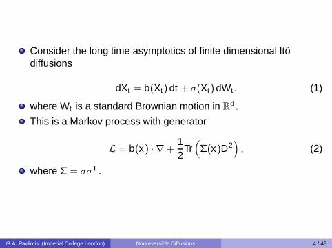
Consider the long time asymptotics of finite dimensional Itôdiffusions

dXt = b(Xt) dt + σ(Xt) dWt , (1)

where Wt is a standard Brownian motion in Rd .

This is a Markov process with generator

L = b(x) · ∇ +12

Tr(

Σ(x)D2)

, (2)

where Σ = σσT .


In order for π(x) to be the invariant distribution of Xt , we requirethat it is the (unique) solution of the stationary Fokker-Planckequation

∇ ·(

−b(x)π(x) +12∇ · (Σ(x)π(x))

)

= 0, (3)

together with appropriate boundary conditions (if we are in abounded domain).

If the detailed balance condition

Js := −bπ +12∇ · (Σπ) = 0, (4)

is satisfied, then the process Xt is reversible wrt π(x).


A stationary diffusion process Xt is reversible (wrt π(x)) if Xt andXT−t have the same law for t ∈ [0,T ].

Time reversibility is equivalent to:◮ The detailed balance condition (4);◮ the generator L being self-adjoint in L2(Rd ;π(x)) (equivalently, the

Fokker-Planck operator L∗ = ∇ · (−b(x) + ∇Σ(x)) beingself-adjoint in L2(Rd ;π−1(x)));

◮ Xt having zero entropy production rate.


There are (infinitely) many reversible diffusions that can be used inorder to sample from π(x):

◮ Either fix b(x) in the detailed balance equation (4) and choose thediffusion matrix Σ(x), or,

◮ fix Σ(x) and choose the drift b(x).

The rate of convergence to equilibrium depends on the tails of thedistribution π(x) and on the choice of diffusion process Xt

(Stramer and Tweedie 1999, Bakry, Cattiaux, Guillin, 2008).

The overdampled Langevin dynamics, Σ = 2I, b(x) = ∇ logπ(x)

dXt = ∇ logπ(Xt) dt +√

2dWt .

is not (always) the best choice.


We can also use higher order Markovian models, for example theunderdamped Langevin dynamics

dqt = pt dt , dpt = ∇ log(π)(qt) dt − γpt dt +√

2γ dWt . (5)

The generator is

L = p · ∇q + ∇q logπ(q) · ∇p + γ(

− p · ∇p + ∆p)

. (6)

We have convergence to the equilibrium distribution

ψ∞(p,q) =1

(2π)N/2Zπ(q)e−p2/2.

The parameter γ > 0 in (5) can be tuned in order to optimize therate of convergence to equilibrium.


To speed up convergence to the target distribution π(x):

Choose optimally (b(x), Σ(x)) within the class of reversiblediffusions.

Consider higher order Markovian models (underdampedLangevin, generalized Langevin equations...) and optimize overthe set of parameters in these models, e.g. the friction coefficientγ.

Consider time dependent temperature (simulated annealing):Holley, Kusuoka, Stroock: Asymptotics of the spectral gap withapplications to the theory of simulated annealing (1989).


To speed up convergence to the target distribution π(x) (contd.):

Choose an appropriate numerical scheme for the solution of theunderlying SDE: Stramer, Tweedie, Langevin-type models. I.Diffusions with given stationary distributions and theirdiscretizations. (1999).

Use a Metropolis-Hastings alrgorithm (acceptance-rejection step):Stramer, Tweedie, Langevin-type models. II. Self-targetingcandidates for MCMC algorithms. (1999).


Choose optimally (b(x), Σ(x)) within the class of reversible diffusions:

Convergence to equilibrium is determined by the first nonzeroeigenvalue of the generator of Xt , which is a self-adjoint operatorin L2(Rd ;π(x)):

λ1 = minφ∈D(L), φ 6=const

〈−Lφ, φ〉‖φ‖2 . (7)

We want to maximize λ1 over the set of drift and diffusioncoefficients that satisfy the detailed balance condition (4). Thisleads to a max-min problem for a self-adjoint operator:

λ1 = maxb,Σ,Js=0

minφ∈D(L), φ 6=const

〈−Lφ, φ〉‖φ‖2 . (8)


If we stay within the class of reversible diffusions then it issufficient to consider spectral optimization problems for selfadjointoperators.

When sampling from multimodal distributions (metastability...) it isreasonable to expect that a well chosen space-dependentdiffusion coefficient can speed up convergence to equilibrium.


Consider the overdamped Langevin dynamics

dXt = −∇V (Xt) dt +√

2β−1 dWt . (9)

The law (PDF) ψt of Xt satisfies the Fokker-Planck equation

∂tψt = ∇ · (∇Vψt + ∇ψt) . (10)

Under appropriate assumptions on the potential, ψ∞ satisfies aPoincaré inequality: there exists λ > 0 such that for all probabilitydensity functions φ,

∫

RN

(

φ

ψ∞− 1

)2

ψ∞dx ≤ 2λ

∫

RN

∣

∣

∣

∣

∇(

φ

ψ∞

)∣

∣

∣

∣

2

ψ∞dx . (11)


The optimal parameter λ in (11) is the spectral gap of theFokker-Planck operator ∇ · (∇V · +∇·), which is self-adjoint inL2(RN , ψ−1

∞ dx).

(11) is equivalent to exponential convergence to equilibrium for (9):for all initial conditions ψ0 ∈ L2(RN , ψ−1

∞ dx), for all times t ≥ 0,

‖ψt − ψ∞‖L2(ψ−1∞ dx)

≤ e−λt‖ψ0 − ψ∞‖L2(ψ−1∞ dx)

, (12)


We will consider the nonreversible dynamics (Hwang et al 1993,2005).

dX bt =

(

−∇V (X bt ) + b(X b

t ))

dt +√

2 dWt , (13)

where b is taken to be divergence-free with respect to theinvariant distribution ψ∞ dx :

∇ ·(

be−V )

= 0. (14)

This ensures that ψ∞(x) dx is still the invariant measure of thedynamics (13).

We can construct such vector fields by taking

b = J∇V , J = −JT . (15)


The dynamics (13) is non-reversible: (X bt )0≤t≤T has the same law

as (X−bT−t)0≤t≤T and thus not the same law as (X b

T−t)0≤t≤T .

Equivalently, the system does not satisfy detailed balance–thestationary probability flux is not zero.

From (15) it is clear that there are many (in fact, infinitely many)different ways for modifying the reversible dynamics withoutchanging the invariant measure.


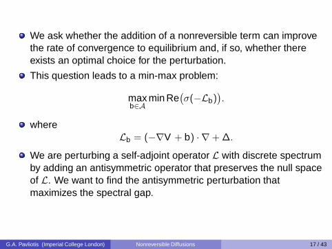
We ask whether the addition of a nonreversible term can improvethe rate of convergence to equilibrium and, if so, whether thereexists an optimal choice for the perturbation.

This question leads to a min-max problem:

maxb∈A

min Re(

σ(−Lb))

.

whereLb = (−∇V + b) · ∇ + ∆.

We are perturbing a self-adjoint operator L with discrete spectrumby adding an antisymmetric operator that preserves the null spaceof L. We want to find the antisymmetric perturbation thatmaximizes the spectral gap.


The reversible case is the worst (Hwang et al 2005):◮ Convergence to equilibrium (measured in L2(Rd , ψ−1

∞)) is slowest

for the reversible case.◮ In other words: the spectral gap is the smallest for the self-adoint

problem.◮ Related work on Poincare and logarithmic Sobolev inequalities for

nonreversible diffusions (Arnold, Carlen, Ju 2008).

Intuition: the addition of a nonreversible (Hamiltonian) partintroduces a drift that can help the system escape frommetastable states.


We consider the nonreversible dynamics

dXt = (−I + δJ)∇V (Xt ) dt +√

2β−1 dWt , (16)

with δ ∈ R and J the standard 2 × 2 antisymmetric matrix, i.e.J12 = 1, J21 = −1. For this class of nonreversible perturbationsthe parameter that we wish to choose in an optimal way is δ.

However, the numerical experiments will illustrate that even anon-optimal choice of δ can significantly accelerate convergenceto equilibrium.

We will use the potential

V (x , y) =14(x2 − 1)2 +

12

y2. (17)


0 0.5 1 1.5 2 2.5 3 3.5 4 4.5 50

0.2

0.4

0.6

0.8

1

1.2

1.4

1.6

1.8

2

t

E(x

2 +y2 )

δ = 0δ =10

Figure: Second moment as a function of time for (16) with the potential (17).We take 0 initial conditions and β−1 = 0.1.


The upper bound for the reversible dynamics (9) is still valid:

‖ψbt − ψ∞‖L2(ψ−1

∞ dx)≤ e−λt‖ψb

0 − ψ∞‖L2(ψ−1∞ dx)

. (18)

Adding a non-reversible part to the dynamics cannot be worsethan the original dynamics (9) (where b = 0) in terms ofexponential rate of convergence.

Our main result is that for a linear drift it is possible to choose b inorder to obtain convergence at exponential rate of the form:

‖ψbt − ψ∞‖L2(ψ−1

∞ dx)≤ C(V , b)e−λt‖ψb

0 − ψ∞‖L2(ψ−1∞ dx)

, (19)

with λ > λ and C(V ,b) > 1.


Let V (x) = 12xT Sx . The nonreversible perturbations that

satisfy (14) are of the form

b(x) = −Ax

A = JS , with J = −JT . (20)

The corresponding SDE is

dX Jt = −(I + J)SX J

t dt +√

2 dWt . (21)

The invariant distribution is

ψ∞(x) =det(S)1/2

(2π)N/2exp

(

−xT Sx2

)

. (22)


Theorem

Define BJ = (I + J)S . Then

maxJ∈AN (R)

min Re (σ(BJ)) =Tr(S)

N. (23)

Furthermore, one can construct matrices Jopt ∈ AN(R) such that themaximum in (23) is attained. The matrix Jopt can be chosen so that thesemigroup associated to BJopt satisfies the bound

∥

∥

∥e−(I+Jopt)St

∥

∥

∥≤ C(1)

N κ(S)1/2 exp(

−Tr(S)

Nt)

, (24)

where κ(S) = ‖S‖ ‖S−1‖ denotes the condition number.


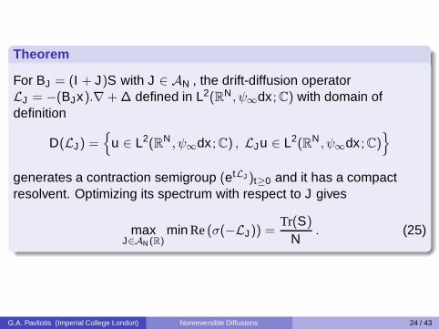
Theorem

For BJ = (I + J)S with J ∈ AN , the drift-diffusion operatorLJ = −(BJx).∇ + ∆ defined in L2(RN , ψ∞dx ; C) with domain ofdefinition

D(LJ) ={

u ∈ L2(RN , ψ∞dx ; C) , LJu ∈ L2(RN , ψ∞dx ; C)}

generates a contraction semigroup (etLJ )t≥0 and it has a compactresolvent. Optimizing its spectrum with respect to J gives

maxJ∈AN (R)

min Re (σ(−LJ)) =Tr(S)

N. (25)


Theorem (contd.)

Furthermore, the maximum in (25) is attained for the matricesJopt ∈ AN(R) constructed as before. The matrix Jopt can be chosen sothat

∥

∥

∥

∥

etLJopt u −(

∫

RNuψ∞dx

)∥

∥

∥

∥

L2(ψ∞dx)

≤ C(2)N κ(S)7/2 exp

(

−Tr(S)

Nt)

∥

∥

∥

∥

u −(

∫

RNuψ∞dx

)∥

∥

∥

∥

L2(ψ∞dx)

(26)

holds for all u ∈ L2(RN , ψ∞dx ; C) and all t ≥ 0.


Corollary

Let us consider the Fokker Planck equation associated to thedynamics (21) on X J

t :

∂tψJt = ∇ ·

(

BJx ψJt + ∇ψJ

t

)

, (27)

where BJ = (I + J)S. Let us assume that ψJ0 ∈ L2(RN , ψ−1

∞ dx). Then,by considering J = −Jopt , where Jopt ∈ AN(R) refers to the matrixconsidered in Theorem 2 to get (26). Then the inequality

∥

∥

∥ψJ

t − ψ∞

∥

∥

∥

L2(ψ−1∞ dx)

≤ C(2)N κ(S)7/2 exp

(

−Tr(S)

Nt)

∥

∥

∥ψJ

0 − ψ∞

∥

∥

∥

L2(ψ−1∞ dx)

,

holds for all t ≥ 0 , when ψ∞ is defined by (22).


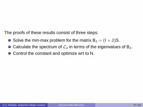
The proofs of these results consist of three steps:

Solve the min-max problem for the matrix BJ = (I + J)S.

Calculate the spectrum of LJ in terms of the eigenvalues of BJ .

Control the constant and optimize wrt to N.


Proposition

Assume that J = S1/2JS1/2 ∈ AN(R) and that S ∈ S>0N (R) . Then the

following two conditions are equivalent:

(i) The matrix BJ = S + J is diagonalizable (in C) and the spectrumof BJ satisfies

σ(BJ) ⊂ Tr(S)

N+ iR . (28)

(ii) There exists a real symmetric positive definite matrix Q = QT

such that

JQ − QJ = −QS − SQ +2Tr(S)

NQ . (29)


Let {λk}Nk=1 denote the (positive real) eigenvalues of Q (counted

with multiplicity), and {ψk}Nk=1 the associated eigenvectors, which

form an orthonormal basis of RN .

Equation (29) is equivalent to the following two conditions: for all kin {1, . . . ,N},

(ψk ,Sψk )R

=Tr(S)

N(30)

and, for all j 6= k in {1, . . . ,N},

(λj − λk )(ψj , Jψk )R = (λk + λj)(ψj ,Sψk )R . (31)

This equivalence enables us to develop an algorithm forcalculating the optimal nonreversible perturbation.


The calculation of the eigenvalues of the matrix in the drift issufficient in order to calculate the spectrum of the generator.Consider the linear SDE (Ornstein-Uhlenbeck process)

dXt = BXt dt + σ dWt (32)

The generator is (with Σ = σσT )

L =12

Tr(

ΣD2)

+ 〈Bx ,∇〉 (33)

Σ can be degenerate, provided that L is hypoelliptic.

We assume that (32) is ergodic with unique Gaussian invariantmeasure π(x) dx .


The spectrum of L in Lp(RN ;π(x)) has been calculated inMetafune, Pallara and Priola, J. Func. Analysis 196 (2002), pp.40-60:For all p > 1 the spectrum consists of integer linear combinationsof the drift matrix. It is independent of the diffusion matrix:

σ(L) =

r∑

j=1

njλj , nj ∈ N

, (34)

where{

λj}r

j=1 denote the r (distinct) eigenvalues of A. Inparticular, the spectral gap of the generator L is determined by theeigenvalues of A.A new proof of this result (for p = 2) can be found in M Ottobre,G.P., K. Pravda-Starov, J. Func. analysis 262(9), 4000-4039(2012).A similar result can also be proved in infinite dimensions: vanNeerven, Infin. Dimens. Anal. Quantum Probab. Relat. Top. 8(2005), no. 3, 473-495.


To prove the exponential convergence for the solution of theFokker-Planck equation and to estimate the constant:

Since LJ is not self-adjoint, in addition to spectral information wealso need estimates on the resolvent.

We use the second quantization formalism (Wick calculus):

−LJ = a∗,T (S − J)a . (35)

where a, a∗ denote creation and annihilation operators.

Use an appropriate expansion in Hermite polynomials.

For the constant in front of the exponential we have that

C(2)N = O(N3).


Algorithm for constructing the optimal nonreversible perturbation

Start from an arbitrary orthonormal basis (ψ1, . . . , ψN).

for n = 1 : N − 1 dobegin

1 Make a permutation of (ψn, . . . , ψN) so that

(ψn,Sψn)R = maxk=n,...,N

(ψk ,Sψk )R > Tr(S)/N

and(ψn+1,Sψn+1)R = min

k=n,...,N(ψk ,Sψk )R < Tr(S)/N .

2 Compute t∗ such that ψt∗ = cos(t∗)ψn + sin(t∗)ψn+1 satisfies(ψt∗ ,Sψt∗)R = Tr(S)/N

3 Use a Gram-Schmidt procedure to change the set of vectors(ψt∗ , ψn+1, . . . , ψN) to an orthonormal basis (ψt∗ , ψn+1, . . . , ψN) .

4 Increase n by one and go back to step 1.

endG.A. Pavliotis (Imperial College London) Nonreversible Diffusions 33 / 43

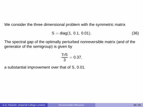
We consider the three dimensional problem with the symmetric matrix

S = diag(1, 0.1, 0.01). (36)

The spectral gap of the optimally perturbed nonreversible matrix (and of thegenerator of the semigroup) is given by

TrS3

= 0.37,

a substantial improvement over that of S, 0.01.


0 10 20 30 40 50 60 70 80 90 10010

−16

10−14

10−12

10−10

10−8

10−6

10−4

10−2

100

102

t

||e−t

B||

BJ

S

Figure: Norms of the matrix exponentials for the 3 × 3 diagonal matrix (36)and its optimal nonreversible perturbation.


We consider a 100 × 100 diagonal matrix with random entries, uniformlydistributed on [0, 1]. For our example the minimum diagonal element (spectralgap) is 0.0012. On the contrary, the spectral gap of BJ with J = Jopt is 0.4762.


0 10 20 30 40 50 60 70 80 90 10010

−20

10−15

10−10

10−5

100

t

||e−t

B||

BJ

S

Figure: Norms of the matrix exponentials for a diagonal matrix with randomuniformly distributed entries and its optimal nonreversible perturbation forN = 100.


Consider a finite difference approximation of the SPDE

∂tu = ∆u + ξ. (37)

We consider this SPDE in 1 dimension on [0, 1] with Dirichlet boundaryconditions.

We can use the finite difference approximation to sample approximatelyfrom an infinite dimensional Gaussian measure.


0 1 2 3 4 5 6 7 8 9 1010

−7

10−6

10−5

10−4

10−3

10−2

10−1

100

101

102

t

||e−t

B||

BJ

S

Figure: Norms of the matrix exponentials for the the discrete Laplacian andits optimal nonreversible perturbation for N = 100.


There are many other stochastic dynamics that can be used in order tosample from a given distribution.

Consider for example the second order Langevin dynamics

q = −∇V (q) − γq +√

2γβ−1W .

For V (q) = 12ω

20q2 the optimal spectral gap is (using (34))

σopt =γ

2, forγ = 2ω0.

We can perturb the Langevin dynamics without changing the invariantmeasure 1

Z e−βH(q,p):

q = p − J∇V (q), p = −∇qV (q) + Jp − Γp +√

2Γβ−1 W .

We have also considered a general symmetric drift matrix Γ instead of ascalar.


Consider the three models

q = −V ′(q) +√

2W , (38a)

q = −V ′(q) − γq +√

2γW , (38b)

q = p, p = −V ′(q) + λz, z = −αz − λp +√

2αW .

(38c)

All these three models can be used in order to sample from thedistribution Z−1e−V (q).

Notice that there are no control parameters in (38a), 1 (the frictioncoefficient) in (38b) and 2 (α and λ) in (38c).

We would like to choose (α, λ) in (38c) in order to optimize the rate ofconvergence to equilibrium.


Figure: Spectral gap as a function of α and λ.


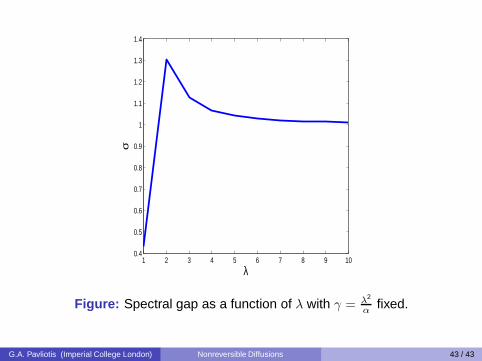
1 2 3 4 5 6 7 8 9 100.4

0.5

0.6

0.7

0.8

0.9

1

1.1

1.2

1.3

1.4

λ

σ

Figure: Spectral gap as a function of λ with γ = λ2

αfixed.


speeding up convergence to equilibrium for diffusion processes · speeding up convergence to...

Documents