speed and position sensorless control of permanent magnet
TRANSCRIPT


Tampereen teknillinen yliopisto. Julkaisu 639 Tampere University of Technology. Publication 639 Matti Eskola Speed and Position Sensorless Control of Permanent Magnet Synchronous Motors in Matrix Converter and Voltage Source Converter Applications Thesis for the degree of Doctor of Technology to be presented with due permission for public examination and criticism in Rakennustalo Building, Auditorium RG202, at Tampere University of Technology, on the 1st of December 2006, at 12 noon. Tampereen teknillinen yliopisto - Tampere University of Technology Tampere 2006

ISBN 952-15-1687-9 (printed) ISBN 952-15-1731-X (PDF) ISSN 1459-2045

iii
Abstract
In this thesis the sensorless control of a permanent magnet synchronous motor (PMSM) is
studied. The study has two main purposes. The first is to find a simple and effective method
to estimate the rotor position and angular speed of the PMSM. The second is to test the
applicability of a matrix converter in sensorless PMSM drives.
A matrix converter (MC) enables a direct frequency conversion without DC-link with
energy storage. In this thesis two matrix converter topologies, direct and indirect, are studied.
The vector modulation and the current commutation strategies of a matrix converter are
described.
Non-ideal properties of frequency converters such as dead times, overlapping times and
voltage losses over semiconductors are disturbances for a control system and position
estimator. These non-idealities are studied and the properties of a conventional voltage source
inverter are compared to direct and indirect MC topologies.
The rotor position and angular speed of the PMSM can be estimated by various methods.
Estimators can be divided into model based estimators and signal injection estimators. Model
based estimators calculate mechanical quantities using the mathematical representation of the
motor. Injection methods usually exploit the saliency of the PMSM. Injected voltage creates
currents which are modulated by the rotor position. The position information can be extracted
from measured currents. In this thesis the best features of model based and injection
estimators are combined. In the proposed hybrid method signal injection is used at low speeds
and the transition to model based estimator is performed when the speed increases. The
estimator methods used in the hybrid estimator are selected by a comparative analysis and
simulations. The most important criteria in the selection of the estimator method in this thesis
are: simple algorithm and no need for modification of the modulator software or frequency
converter.
The suitability of the proposed hybrid estimator is tested by simulations and experimental
tests in various operating conditions. To test the performance of the matrix converter the
experiments are carried out using both MC topologies and a conventional voltage source
converter.
The results obtained show that a matrix converter can be used in PMSM drives where the
speed and position of the PMSM are not measured. The proposed estimator method is stable
over the nominal speed range including the zero speed region with full load torque.

iv

v
Preface
This work was carried out at the Institute of Power Electronics at Tampere University of
Technology (TUT) during the years 2001-2006. The research was funded by the Graduate
School in Electrical Engineering, TUT, the Finnish Funding Agency for Technology and
Innovation (TEKES) and industrial partners (ABB Oy Drives, Hyvinkään TechVilla, Kalmar
Industries, KCI Konecranes Oyj, Kone Oyj, Vacon Oyj). I am also very grateful for the
financial support in the form of personal grants from the Foundation of Technology
(Tekniikan edistämissäätiö).
I express my gratitude to Professor Heikki Tuusa, the head of the Institute of Power
Electronics, for supervising my thesis work and providing an excellent research enviroment. I
thank all the staff in the Institute of Power Electronics for providing with me a pleasant
working atmosphere. I am thankful to Tero Viitanen Dr. Tech. and Mikko Routimo Lic. Tech.
for providing answers to my questions regarding voltage source converters. I also thank Mika
Salo Dr. Tech. for the microcontroller support. Laboratory technician Pentti Kivinen built all
the excellent test benches for the PMSM drives used in this thesis work, which is greatly
appreciated. The matrix converter research of this thesis was done in collaboration with Matti
Jussila Lic. Tech. Special thanks to Matti who built the matrix converter prototypes and did
all the dirty work behind the results regarding MCs. Furthermore, I thank professors Jorma
Luomi and Juha Pyrhönen for their comments and for reviewing this thesis.
I wish also to thank my parents and little brother for their encouragement and support
during the past years. Above all, I express my deepest thanks to my wife, Mirkka, for her
love, patience and understanding. And finally, very special thanks to our sunshine, Elsa, for
many joyful moments during the completion of this thesis.
Helsinki, November 2006
Matti Eskola

vi

vii
Contents
Abstract .................................................................................................................. iii
Preface ................................................................................................................... v
Contents ................................................................................................................. vii
List of symbols .................................................................................................................. ix
1 Introduction ................................................................................................................... 1 2 Frequency converter fed PMSM drive .............................................................................. 6 2.1 Permanent magnet synchronous machines .................................................................. 6 2.2 Modelling of the PMSM .............................................................................................. 8 2.2.1 Modelling of the voltage equations using the space-vector theory ......................... 8 2.2.2 A PMSM model with higher order flux linkage harmonics.................................. 13 2.3 Pulse width modulated frequency converters ............................................................ 18 2.3.1 Voltage source converter....................................................................................... 19 2.3.2 Matrix converter .................................................................................................... 22 2.4 Comparison of non-ideal properties of VSC and MC................................................ 32 2.4.1 Non-linear model of the bi-directional switch ...................................................... 32 2.4.2 Non-linear model of the VSI ................................................................................. 33 2.4.3 Non-linear model of the IMC................................................................................ 35 2.4.4 Non-linear model of the DMC .............................................................................. 39 2.4.5 Comparison of topologies ..................................................................................... 41 2.5 Control system of the PMSM..................................................................................... 44 3 Model based estimators..................................................................................................... 48
3.1 Introduction to speed and position estimators............................................................ 48 3.1.1 Basic properties of the estimators ......................................................................... 49 3.1.2 Principles of the comparison of the estimators in this study................................. 50
3.2 State observers ........................................................................................................... 51 3.2.1 State observers using a linearized PMSM model .................................................. 52 3.2.2 Non-linear state observer....................................................................................... 55 3.2.3 Stochastic state observer (Kalman filter) .............................................................. 56 3.2.4 General properties of state observers in sensorless control of PMSM.................. 58
3.3 Phase locked loop structure in sensorless control of PMSM..................................... 59 3.4 Back-emf estimators .................................................................................................. 62
3.4.1 Direct speed and position estimation..................................................................... 63 3.4.2 Voltage equations in the estimated synchronous reference frame ........................ 66 3.4.3 Back-emf estimator with the phase locked loop structure .................................... 68 3.4.4 Back-emf estimator based on the current tracking................................................ 73 3.4.5 Combined back-emf estimator .............................................................................. 76

viii
3.5 Flux linkage estimators .............................................................................................. 77 3.5.1 Estimation of the flux linkage ............................................................................... 77 3.5.2 Speed and position estimation............................................................................... 79 3.5.3 Drift correction methods ....................................................................................... 80
3.6 Comparison of the model based estimators by simulations....................................... 88 3.6.1 Simulations with ideal PMSM drive ..................................................................... 88 3.6.2 Simulations with non-ideal PMSM drive.............................................................. 99 3.6.3 Conclusions of simulations ................................................................................. 105
4 Signal injection estimators.............................................................................................. 107 4.1 Introduction to signal injection estimators............................................................... 107
4.1.1 Injection estimators based on the saliency of the PMSM ................................... 107 4.1.2 Injection estimators based on mechanical oscillation ......................................... 110
4.2 Estimators using continuous high frequency signal injection.................................. 111 4.2.1 d,q injection (alternating injection)...................................................................... 111 4.2.2 α,β injection (revolving injection)....................................................................... 114 4.2.3 The effect of non-ideal drive ............................................................................... 115 4.2.4 Compensation of disturbances and other practical aspects.................................. 119 4.2.5 Tuning of the signal injection estimator.............................................................. 121 4.3 Low frequency signal injection estimator................................................................ 123 4.3.1 Low frequency d,q injection ................................................................................ 123 4.3.2 Analysis of the steady state behaviour................................................................. 125 4.3.3 Compensation of the steady state position error.................................................. 129 4.4 Hybrid estimator ...................................................................................................... 130 4.5 Simulations of injection and hybrid estimators........................................................ 132 4.5.1 Low speed simulations......................................................................................... 133 4.5.2 Nominal speed simulations.................................................................................. 135
5 Realisation of the experimental setup............................................................................ 137 5.1 Experimental VSI drive ........................................................................................... 137 5.2 Experimental matrix converter drive ....................................................................... 138 5.2.1 Indirect matrix converter prototype...................................................................... 139 5.2.2 Direct matrix converter prototype ........................................................................ 141 5.3 Software implementation ......................................................................................... 142
6 Operation of the sensorless PMSM drives ..................................................................... 144 6.1 Model based estimator ............................................................................................. 144 6.2 Injection and hybrid estimators................................................................................ 146 6.2.1 Comparison of VSI and IMC, d,q injection......................................................... 146 6.2.2 Hybrid estimator .................................................................................................. 147 6.3 Summary of the results ............................................................................................ 154 7 Conclusions ............................................................................................................... 156 References ............................................................................................................... 158 Appendix A ............................................................................................................... 168 Appendix B ............................................................................................................... 169

ix
List of symbols a Acceleration AC Alternating Current b Friction constant BP Band Pass BS Band Stop d Relative duration of vector in PWM DC Direct Current DMC Direct Matrix Converter e Back-emf (electromotive force) EKF Extended Kalman Filter ELO Extended Luenberger Observer f Frequency i Current IGBT Insulated Gate Bipolar Transistor IMC Indirect Matrix Converter j Imaginary unit g Gain parameter k, K Gain parameter L Inductance LP Low Pass m Modulation index MC Matrix Converter p Number of pole pairs PI Proportional and Integrating controller PLL Phase Locked Loop PM Permanent Magnet PWM Pulse Width Modulation R Resistance SVM Space Vector Modulation sw Switching function t Time T Torque TF Transfer Function VSI Voltage Source Inverter VSC Voltage Source (frequency) Converter W Energy u Voltage x Arbitrary quantity ∆ Voltage error of a frequency converter δ Load angle ε Error signal θ Position angle ρ Coefficient used to determine poles of a PLL ψ Flux linkage ω Angular frequency
Subscripts abc Vector or matrix of a three-phase quantity

x
a,b,c Input phases of the frequency converter, phases of three phase quantities A,B,C Ouput phases of the frequency converter ave Average value c Current model, overlapping d Real part of the space-vector in the rotor reference frame de Real part of the space-vector in the estimated rotor reference frame e Electrical quantity i A quantity oscillating with injection frequency, integration, input id, iq Real and imaginary parts of space-vector quantity with injection frequency in
the rotor reference frame ide, iqe Real and imaginary parts of space-vector quantity with injection frequency in
the estimated rotor reference frame inv Inverse transformation L Load LL Line-to-Line on On-state loss q Imaginary part of the space-vector in the rotor reference frame qe Imaginary part of the space-vector in the estimated rotor reference frame mech Mechanical quantity mod Modulation period n Nominal value o Output p Proportional r Electric rotor quantity (position angle, angular speed) ref Reference signal s Sample period supply Mains (three-phase distribution network) sw Switching period in PWM α Real part of the space-vector in the stationary reference frame β Imaginary part of the space-vector in the stationary reference frame δ Lead vector of the line bridge γ Lag vector of the line bridge λ Lead vector of the load bridge κ Lag vector of the load bridge 2 Output of the direct speed estimator
Superscripts g General reference frame (notation used with complex phasor, e.g. ig) r Rotor reference frame (notation used with complex phasor, e.g. ir) re Estimated rotor reference frame (notation used with complex phasor, e.g. ire) s Stationary reference frame T Transpose * Complex conjugate
Other notations x Estimated value of x x~ Estimation error (x - x ) of x x Matrix or vector x x Complex phasor, space-vector

1. Introduction
DC motor drives dominated the field of variable speed drives from the 19th century to the
last decades of the 20th century. The controllability of DC drives was superior to those of AC
drives. At the end of the 1960s K. Hasse introduced the field oriented control of AC motor. It
was pointed out that in theory the induction motor can be controlled in the same way as the
DC motor. The development of semiconductor power devices made it possible to build
frequency converters for AC motors allowing a sinusoidal three-phase current supply with
continuous frequency control. In the 1980s frequency converter fed AC drives using field
oriented control were ready to challenge DC drives commercially. Since then the percentual
share of DC drives has declined because the AC motor has several benefits compared to the
DC motor. It is cheaper and needs much less maintenance because no mechanical commutator
is needed. The speed range of the AC motor is wider and the machine size is smaller in the
same power class. At present the frequency converter fed induction machine is the most
common choice in industry when adjustable speed operation is required in power range from
a few hundred W to a few MW.
The synchronous machines are the other group of AC machines and possess many of the
advantages of induction machines. Traditionally the use of DC excited synchronous machines
has been limited to generators and other high power applications. They cannot compete with
induction motors in medium power range drives due to the higher price and more complex
structure.
If DC excited rotor winding is replaced by permanent magnets, the synchronous machine
has many attractive features compared to the induction motors. The excitation winding is not
needed in the rotor. Thus the structure is greatly simplified. The copper losses are reduced
because there are no current circuits in the rotor. This ensures higher efficiency and easier
cooling compared to the induction motor. The use of modern rare-earth magnetic materials
enables high flux densities and facilitates the construction of motors with unsurpassed power
density. Permanent magnets can be manufactured in many shapes, which allows great
flexibility for motor construction. The major drawback of the permanent magnet synchronous
machine (PMSM) is the price. The stator structure is often similar to that of induction motors
but the magnetic materials needed in the rotor are still fairly expensive. However, PMSMs are

Introduction 2
becoming more popular and their application range is widening. Usually PMSMs are used in
high performance low power servo applications. In recent years PMSMs have also been
utilised in paper mills, wind-energy applications, elevators, ship propulsion drives and other
high power applications. It is expected that in future PMSMs will continue replacing
induction motors, also in conventional variable speed drives.
In variable speed PMSM drives the motor is controlled by a frequency converter. In the
low and middle power ranges the most common solution in industry is to use a voltage source
PWM inverter with diode rectifier. If the power quality is concerned the rectification is also
carried out by an active PWM bridge. The active rectifier enables bi-directional power flow.
This saves energy if the machine also operates in the regenerating region. In the case of the
diode rectifier the power must be dissipated in a brake resistor if the machine is regenerating.
In a DC link between the rectifier and an inverter the capacitor is used as an energy storage.
Smoothening of the rectified voltage is the other purpose of the capacitor.
In recent years research on direct frequency conversion using a matrix converter (MC) has
become more intense. The main reason for the interest in the matrix converter is that it
provides a compact solution for a four-quadrant frequency converter, which produces
sinusoidal input and output currents without a DC-link with passive components. The absence
of the DC-link also has its disadvantages. Unfiltered input and output disturbances are carried
through MC and output/input voltage ratio is smaller compared to the voltage source
converter (VSC). MCs enabling the four-quadrant operation can be divided into direct and
indirect topologies. The direct matrix converter (DMC) is a conventional MC circuit [Ven80]
without the DC-link. Indirect matrix converter (IMC) consists of separated line and load
bridges [Min93]. However, there exists no capacitor or inductor as an energy storage between
the bridges.
The reduction of the size of the variable speed drive components is always an important
goal in industry. In the future the frequency converter may be integrated into the motor. Due
to the compact structure the integration of the matrix converter should be more realisable than
the integration of conventional converters with DC-link. It will be interesting to see if MCs
can challenge the VSC with an active rectifier. VSCs are mature technology but their size and
costs have also been reduced due to the development of semiconductors and capacitors.
The field oriented control (FOC) originally introduced for induction machines is also the
most common control strategy in PMSM drives. FOC is also called vector control [Nov00].
This term is used in this thesis. In vector control the torque of the machine is controlled via

3
controlling the stator current vector. The outer control system adjusting the speed and position
gives the torque demand for the current control system.
Twenty years ago the direct torque control method (DTC) was introduced [Tak86]. This is
the other widespread control method for AC drives. In a DTC drive the idea is to control the
stator flux linkage and torque directly, not via controlling the stator current. This is
accomplished by controlling the power switches using a predefined “optimum switching
table” to select appropriate voltages for a motor. The selection of the switching states is made
by the hysteresis comparators for torque and stator flux linkage. [Luu00] analyses the
application of DTC to PMSMs. Direct torque control of the PMSM is beyond the scope of
this thesis.
The vector control of a synchronous machine requires knowledge of the rotor position and
angular speed. These mechanical quantities of a PMSM have usually been measured by shaft
mounted motion sensors e.g. a tachometer, an encoder or a resolver. The presence of these
sensors implies several disadvantages due to additional cost, a higher number of connections
between the motor and the frequency converter and reduced robustness. In an industrial
environment the sensors are vulnerable to mechanical impacts. Especially in lower power
ranges the motion sensor can be the most expensive component in the entire drive system. For
this reason several strategies to detect the speed and position without sensors have been
developed for synchronous and asynchronous machines during the last twenty years.
If the speed and position are detected by estimator algorithms instead of motion sensors the
control system of the AC machine is said to be sensorless. Sensorless control is a somewhat
misleading term because only the speed/position control system is sensorless. The phase
currents of the PMSM are measured for current control in vector control system. The term
“indirect control” is also used in some publications [Yin03]. However, sensorless control is an
established term in the literature and is also used in this thesis.
The position and speed estimators can be divided into two groups. The majority of the
papers published describe methods based on the mathematical model of the PMSM [Bol99],
[Jon89], [Mat96]. The main drawback of these model based estimators is insufficient
performance at low speeds. To overcome low speed stability problems extensive research has
been carried out to develop so-called injection estimators. In these methods a high frequency
signal (voltage or current) is injected into the motor and the position angle and speed are
determined by processing the resulting currents or voltages [Cor98], [Jan95], [Jan03], [Sil03].

Introduction 4
The objective of this study has been to find a simple and effective method for on-line
estimation of the rotor position angle and angular speed of the PMSM and to study the
suitability of the matrix converter for the sensorless PMSM drives. The most promising speed
and position estimators presented in the literature and meeting the following four
requirements are compared.
1. Modification of the hardware of the frequency converter is not required.
2. Modification of the space-vector modulator software is not required.
3. The algorithm of the estimator should be as simple as possible.
4. The drive must be stable over the entire speed range including operation at zero speed.
Special attention was paid to zero speed region, which is the most problematic operating
region for model based speed and position estimators. Injection estimators are stable at zero
speed region. Therefore a combination of a model based method and an injection method is
one of the goals of this thesis. The combination can exploit the strengths of both classes of
estimators. The other goal is to empirically prove that the matrix converter can be applied in
PMSM drive with sensorless control.
In Chapter 2, the modelling of the variable speed drive with PMSM is studied. The
properties of the PMSMs are briefly discussed. The PMSM model taking the flux linkage
harmonics into account is presented. The model is used in the simulations presented in
Chapters 3 and 4. The voltage source frequency converter and matrix converter topologies
and their non-ideal properties are studied [Jus06]. The vector control of the PMSM used in
this thesis is described.
In Chapter 3, model based speed and position estimators (observers, flux estimators and
back-emf estimators) are studied and the most promising methods are compared in
simulations. The methods presented by Matsui [Mat90], [Mat92] were selected for further
development. A new method which combines the best properties of Matsui’s estimators is
presented. This new algorithm is used in the hybrid estimator presented in Chapter 4.
In Chapter 4, signal injection estimators are studied. The high frequency signal injection
methods are compared. The effect of the reference frame is studied. In addition to high
frequency methods the low frequency estimator is studied [Esk05]. This method was
introduced in 2001 for induction motors [Lep03] and is applied to PMSM drive in this study.
The high frequency method where sinusoidal voltage is injected in the rotor reference frame is
selected for the final implementation. At the end of Chapter 4 the model based estimator and

5
signal injection estimator are combined to achieve stable operation over the entire speed range
of the PMSM.
In Chapter 5, the experimental setup is presented. The performance of the proposed
sensorless control method is verified in Chapter 6. The matrix converter fed speed and
position sensorless PMSM drive is tested experimentally. Some tests are also carried out by
the voltage source converter and the results are compared to those achieved by MCs. Chapter
7 concludes the study.
The contributions of this thesis are summarized below.
- The analysis and comparison of output voltage non-idealities of matrix converters
(Chapter 2). The results were published in [Jus06]. The author’s contribution was
developing the simulation model in collaboration with Jussila and programming of the
control software for the PMSM drive used in experimental tests.
- A novel model based estimator algorithm is presented in Section 3.4.5. The proposed
algorithm is based on the work of Matsui [Mat90], [Mat92]. In this thesis the best
features of Matsui’s estimators are combined.
- Problems arise due to the saliency when the low frequency injection is used to estimate
the speed and position of the PMSM. The saliency effect is theoretically analysed and a
simple compensation method is proposed (Chapter 4). The performance of the
compensation method is verified experimentally. The results were published in
[Esk05]. Speed and position estimator using the low frequency injection was originally
presented for induction motors in [Lep03].
- The proposed hybrid estimator is proven to be stable in the speed range from zero to
nominal speed.
- It is shown by measurements in Chapter 6 that matrix converters can be applied in
PMSM drives where the rotor angular speed and position are not measured. Both MC
topologies are experimentally tested. The PMSM drive fed by the direct MC topology
with sensorless control has been reported in [Ari04] and [Liu03]. The indirect MC
topology with sensorless control was tested first time in [Esk04].

2. Frequency converter fed PMSM drive
2.1 Permanent magnet synchronous machines
Permanent magnet synchronous machines can be divided into brushless DC machines
(BLDC) and sinewave machines. The following ideal characteristics of BLDC are given in
[Hen94].
- Distribution of magnet flux in the airgap is rectangular,
- The current waveform of three phase BLDC is a 120° squarewave. Two phases are
conducting at any and every instant,
- Stator windings are concentrated.
The ideal characteristics of sinewave PMSM are:
- Sinusoidal distribution of magnet flux in the airgap,
- Sinusoidal current waveforms,
- Sinusoidal distribution of stator conductors.
The control of a power electronic device feeding the BLDC is easier than the control of a
converter using PWM techniques. Demands for semiconductor switches and control
electronics are lower compared to a frequency converter capable of producing sinusoidal
currents. The development of semiconductors and integrated circuits has increased the
popularity of sinewave machines. A sinewave machine fed by a modern frequency converter
has clearly better torque characteristics compared to BLDC drive. BLDC drives are not
discussed further in this study.
PMSMs can be categorized based on the mounting of the permanent magnets. Fig. 2.1a
shows one possible rotor structure with two pole pairs. The magnets are mounted on the
surface of the rotor (SPMSM). Fig. 2.1b shows one possible structure where magnets are
buried inside the rotor (IPMSM). More detailed information from different magnet mounting
strategies and rotor structures will be found in [Hen94].

7
q d
NN
S
S
q d
N
N
S
S
N
NS S
a) b) Fig. 2.1 a) PMSM with surface mounted magnets, two pole pairs. b) PMSM with interior mounted
magnets, two pole pairs.
In Fig. 2.1 arrows with “d” and “q” denote direct and quadrature axes of the PMSM. d-axis
is the magnetic axis of the rotor and the arrow indicates the positive direction of the rotor flux.
The mechanical angle between d and q axes is π/(2p) where p is the number of pole pairs.
If the magnets are mounted on the rotor surface the effective air gap is rather large because
the permeability of permanent magnets is low, typically close to that of air [Hen94]. Due to
the large air gap the inductances of the SPMSMs are smaller. The difference between the
direct and quadrature axis inductances (Ld and Lq) is usually small. However, there is always
some saliency because the strong magnetic fields saturate the iron, especially the stator teeth.
This makes the effective air gap larger in the d-axis direction. Thus Ld < Lq. Due to the
relatively small inductances PMSMs with surface mounted magnets are not suitable for drives
where strong field weakening is required.
In the case of IPMSMs there are flux paths in the d axis direction where the reluctance is
high due to the low permeability of the permanent magnet material, Fig. 2.1b. Thus the
inductance is clearly larger in the q axis direction. The buried magnet placement enables a
small air gap. Thus the inductances are larger compared to a SPMSM.
PMSMs can be also categorized on the basis of the direction of the flux. Fig. 2.1 and Fig.
2.2a show the structure of a radial flux machine, which is the common structure for AC
machines. The flux created by the permanent magnets crosses the air gap in a radial direction
to link the rotor flux with stator windings. The stator structure of the radial flux PMSM is
basically same as in the case of the induction machines. The flux can also cross the air gap in
parallel direction with the rotor shaft, Fig. 2.2b. These machines are called axial flux
machines.

Frequency converter fed PMSM drives
8
a)
b)
Fig. 2.2 a) Radial flux structure and b) axial flux structure.
A small length/diameter ratio is typical of axial flux machines. This structure makes
possible a high number of pole pairs. Axial flux machines are often used in high power
solutions where angular speeds are rather small, e.g. elevators, generators and ship propulsion
drives. Radial flux machines compete with induction motors in variable speed drives in
industrial applications and are extensively used in small power servo drives.
2.2 Modelling of the PMSM
At the beginning of Section 2.2.1 three-phase voltage and flux linkage equations of the
PMSM are given. Section 2.2.1 also provides a short introduction to space-vector theory and
its application on modelling of PMSMs. Section 2.2.2 deals with the PMSM model, where the
effects of flux linkage harmonics are taken into account.
2.2.1 Modelling of the voltage equations using the space-vector theory
The voltage equations of the three-phase PMSM in a phase variable form are [Vas92],
[Nov00]
dtd
Riu
dtd
Riu
dtd
Riu
ccc
bbb
aaa
ψ
ψ
ψ
+=
+=
+=
(2–1)
The flux linkages can be written
)π/32cos()()()()π/32cos()()()(
)cos()()()(
rmbrcbm,arcam,crscc
rmcrbcm,arbam,brsbb
rmcracm,brabm,arsaa
++++=
−+++=
+++=
θψθθθψθψθθθψθψθθθψ
iLiLiLiLiLiLiLiLiL
(2–2)

9
where Lsa, Lsb and Lsc are self inductances of the stator windings and Lm,ca, Lm,ab ans Lm,bc are
mutual inductances between the windings. ψm is a permanent magnet (PM) flux. Due to the
saturation effects and mechanical structures of PMSMs the inductances are functions of the
electric rotor position angle θr. The electric rotor position angle is the direction of the rotor
flux (North Pole of the rotor magnets). The zero angle is the direction of phase a. The relation
between the mechanical and the electrical rotor position is
mechr θθ p= (2–3)
where p is the number of pole pairs.
In a general case the inductances of the PMSM (2–2) can be expressed with Fourier series
[Low96], [Pet01]. The inductances consist of a constant component and a sum of even
harmonics when the rotor position θr changes.
In the literature on controlled AC drives the following assumptions are commonly made
[Vas92].
- The stator windings are assumed to be perfectly sinusoidally distributed,
- The effect of the discrete nature of the stator structure is neglected. Therefore stator
windings produce a sinusoidal magneto-motive-force,
- In the case of the PMSM the radial flux-density distribution produced by the rotor
permanent magnets is perfectly sinusoidal and the flux linkage from the rotor in the
stator windings contains only the fundamental component,
- The effect of the magnetic saturation is ignored.
With these assumptions the inductance variation has only a one sinusoidal component. The
inductance of the phase is at its minimum when the rotor flux direction (d axis in Fig. 2.1) is
in alignment with the phase. Thus the phase inductances are functions of the angle 2θr. If only
this single sinusoidally distributed saliency is assumed, the self inductances and the mutual
inductances of a synchronous motor are written [Vas92]:
)3/2()()3/2()(
)2cos()(
r2s0srsc
r2s0srsb
r2s0srsa
πθθπθθ
θθ
++=−+=
+=
LLLLLLLLL
(2–4)
)2cos()(
)3/π22cos()()3/π22cos()(
rm2m0rbcm,
rm2m0rcam,
rm2m0rabm,
θθθθθθ
LLLLLLLLL
+=
++=
−+=
(2–5)
where Ls0 and Lm0 are the average components of the self and the mutual inductances. Ls2 and

Frequency converter fed PMSM drives
10
Lm2 are the amplitudes of the sinusoidal components. In the case of PMSMs Ls2<0 and Lm2<0.
In a general case the flux linkages created by the permanent magnets consist of a
fundamental sinusoidal component and the sum of odd harmonics. If the assumptions given
above are valid the three-phase flux linkage created by the PM flux has only the fundamental
component as written in (2–2).
2.2.1.1 Space-vector theory
In the theory and analysis of AC systems a commonly used approach is to represent the
three-phase quantities as a function of time by complex phasors. These phasors are called
space-vectors in the literature. This section gives a short introduction to space-vector theory.
More detailed information will be found in many textbooks, e.g. [Vas92], [Kra02], [Nov00].
The Park transformation matrix K transforms the three phase quantity x into a complex
phasor called a space-vector. x denotes any three phase quantity, current, flux linkage or
voltage. Subscripts α and β denote real and imaginary parts of the space-vector.
⎥⎥⎥
⎦
⎤
⎢⎢⎢
⎣
⎡
⎥⎥⎥
⎦
⎤
⎢⎢⎢
⎣
⎡+−−−−
+−=
⎥⎥⎥
⎦
⎤
⎢⎢⎢
⎣
⎡
c
b
a
0
β
α
2/12/12/1)3/π2sin()3/π2sin(sin
)3/π2cos()3/π2cos(cos
32
xxx
xxx
44444444 344444444 21K
θθθθθθ
(2–6)
In (2–6) θ denotes the angle of the real axis of the complex plane compared to the direction of
the phase a. This angle of the reference frame can be freely selected. It may be constant or a
function of time. The coefficient 2/3 in front of the transformation matrix means that the non-
power invariant form of coordinate transformation is used. In that case the length of the
space-vector xα + jxβ is equal to the peak value of the sinusoidal three phase quantity x. This
method is used throughout this study. The other common form of transformation [Vas92] is to
replace 2/3 by its square root. In that case the amplitude is changed but the power and torque
equations in space-vector form need no additional coefficients. When the non-power invariant
(amplitude invariant) form is used the inverse transformation is
⎥⎥⎥
⎦
⎤
⎢⎢⎢
⎣
⎡
⎥⎥⎥
⎦
⎤
⎢⎢⎢
⎣
⎡
+−+−−−
−=
⎥⎥⎥
⎦
⎤
⎢⎢⎢
⎣
⎡
0
β
α
c
b
a
inv
1)3/π2sin()3/π2cos(1)3/π2sin()3/π2cos(1sincos
xxx
xxx
4444444 34444444 21K
θθθθ
θθ (2–7)
In this thesis the star connection is used in all machines. If the neutral point is not
connected the zero sequence component x0 has non-zero value only under fault conditions.

11
Fault conditions are not covered in this work. If x is voltage in (2–7) the sum of the
fundamental frequency components of ua, ub and uc is approximately zero. In PWM operation
the instantaneous sum of the phase voltages is not zero because at every instant each three
motor phases are connected to either lower or higher voltage level. As will be explained in
Section 2.3 these two voltage levels can be DC-buses or phase voltages of the supply
network. This zero sequency voltage component varying with high frequency is not
interesting when sensorless control methods are analysed. Therefore x0 is assumed to be zero
throughout this study.
In PMSM drives the typical choices for the angle of the reference frame θ (2–6) are 0 and
the rotor position angle θ r . If the angle is zero the transformation is made to the stator
reference frame, where the real axis is aligned in the direction of phase a. Because the
position angle is constantly zero it is also called a stationary reference frame. In the original
Park transformation the real axis of the complex plane is tied to the rotor position θ r . In this
thesis it is called rotor reference frame.
When sensorless control methods are studied θ r is unknown. In that case θ r is replaced by
its estimate θ r in (2–6). The real and imaginary parts of the space-vector are denoted by the
subscripts d and q in the rotor reference frame and by de and qe in the estimated rotor frame.
In the stationary frame the real and imaginary parts are marked by α and β. In the literature
they are also denoted by D and Q. The coordinate transformations are illustrated in Fig. 2.3 .
α
β
2π/3
a)
d
qe
de
q
θr~
θθr
rα
c)
β
ide
iiqe iq
id
iaib
ic i
iα
iβ
α
β i
iα
iβ
b)
d
q
θridiq
Fig. 2.3 a) Composition of the current vector from three phase form to space-vector representation. b) Transformation from stationary to rotor reference frame. c) Transformation between actual and
estimated rotor reference frames.
If a complex phasor notation is used the transformation to stationary frame can be written
using (2–6) with θ = 0.
βαcb
cba/3j4
c/3j2
bas j
3j)(
21
32)ee(
32 iiiiiiiiiii π +=⎟
⎠⎞
⎜⎝⎛ −+⎟
⎠⎞
⎜⎝⎛ −−+=++= π (2–8)

Frequency converter fed PMSM drives
12
where ia, ib and ic are phase currents. A similar expression can also be written for voltage and
flux linkages. If no zero-sequence currents exist iα = ia. Using complex quantities the
transformation between stationary and rotating reference frames can be written
)sincos(j)sincos(j
)sincos(j)sincos(j
rdrqrqrdβαrs
rαrβrβrαqdsr
r
r
θθθθ
θθθθθ
θ
iiiiiieii
iiiiiieiij
j
++−=+==
−++=+== −
(2–9)
The superscripts s and r of the phasors in (2–8) - (2–9) indicate the reference frame. In the
literature on AC motors s and r often indicate stator and rotor quantities when used as
subscripts. This thesis deals with PMSMs without damper windings. Thus there is no
confusion even if the subscripts s and r are omitted in the case of three-phase quantities.
2.2.1.2 Space-vector representation of voltage and flux linkage equations
The model of the PMSM is simplified if the three-phase voltage model (2–1) is
transformed to a space-vector form using (2–6). In rotor reference frame the voltage equation
of the PMSM is:
drq
qrd
dd
ψωψ
ψωψ
++=
−+=
dtd
Riu
dtd
Riu (2–10)
Flux linkage components ψd and ψq are achieved by transforming (2–2) to the rotor reference
frame. If the inductances (2–4), (2–5) contain only the sinusoidal component varying as a
function of 2θr the flux linkage in the rotor reference frame is
qqq
ddmd
iLiL
=+=
ψψψ
(2–11)
where Ld = Ls0 - Lm0 + Ls2/2 + Lm2 and Lq = Ls0 - Lm0 - Ls2/2 - Lm2. When (2–11) is substituted
into (2–10) the voltage equation of the PMSM can be written
)( ddmr
qqqq
qqrd
ddd
iLdtdi
LRiu
iLdtdi
LRiu
+++=
−+=
ψω
ω (2–12)
The voltage equation (2–12) is usually applied in the literature. It is accurate enough when the
performance of the control system is analysed. A more accurate voltage model of the PMSM

13
is studied in Section 2.2.2. The equations of the electromagnetic torque and mechanics are
given in Section 2.2.2.3.
About the notations
The three-phase equations transformed into the space-vector form can be written using the
matrix notation or the complex phasor notation. The complex phasor form is possible only if
the parameters of the phases are equal. In the case of an AC motor this means that R and L are
equal in each phase and do not vary as a function of rotor position. The basic stator voltage
equation of the symmetric PMSM in the rotor frame is used as an example. It can be written
using the complex phasor notation as follows
)(j mr
r
rrr ψω +++= iL
dtidLiRu (2–13)
In (2–12) the direct and quadrature axis inductances are not equal. Now the
aforementioned simple notation cannot be used. The voltage equation can be written in matrix
form:
)( mr
rrrr ψLiTiLRiu +++= ω
dtd (2–14)
⎥⎦
⎤⎢⎣
⎡=⎥
⎦
⎤⎢⎣
⎡ −=⎥
⎦
⎤⎢⎣
⎡=⎥
⎦
⎤⎢⎣
⎡=⎥
⎦
⎤⎢⎣
⎡=⎥
⎦
⎤⎢⎣
⎡=
0,
0110
,0
0,
00
,, mm
q
d
q
drq
dr ψψTLRiu
LL
RR
ii
uu
or the real and imaginary parts are written separately as in (2–12). The matrix notation (2–14)
is compact and often used in many papers to save space. It is the opinion of the author that
Equation (2–12) is more informative because the real and imaginary parts are written
separately. In this study the style of Equation (2–12) is preferred.
2.2.2 A PMSM model with higher order flux linkage harmonics
The assumptions given in the beginning of Section 2.2.1 can be made if the PMSM is
modelled for control system analysis. If the electric angular speed ω r = pωme c h and the
position angle of the rotor θr are measured using a sensor the modern high performance
closed-loop control techniques compensate most of the effects of non-ideal machine structure.
In the literature the non-ideal properties of the PMSMs are usually analysed in papers
addressing torque ripple minimization in high performance drives with speed and position
sensors [Col99], [Hol96], [Low90], [Qia04].
In this thesis sensorless control is applied. This means that the speed and position are

Frequency converter fed PMSM drives
14
determined using current and voltage information. These electrical quantities contain the
harmonics caused by non-ideal properties of the machine and the frequency converter. To
understand the performance and the problems of sensorless methods a more accurate PMSM
model must be used.
The model now presented is still simplified compared to the real PMSM.
- The effects of magnetic saturation and motor temperature are ignored,
- Slot harmonics (cogging torque) are not modelled. The reluctance of the magnetic
circuit varies when the edges of the rotor magnets pass the stator teeth. Torque
pulsation occur at a frequency ωmech × number of slots,
- The phase resistances are assumed to be identical,
- Geometric symmetry of the stator and rotor poles is assumed.
2.2.2.1 Phase inductances of the PMSM
If all the simplifications given above and in Section 2.2.1 are used the phase inductances
contain only the average value Ls0 = (Lq + Ld)/2 and sinusoidal component with frequency 2ω r
and amplitude Ls2 = (Ld - Lq)/2. This sinusoidal component is called main saliency. If a more
accurate model is needed the higher order saliencies must be included. In a general case the
self inductances of phases are [Low96], [Pet01]
)3/2()()3/2()(
)2cos()(
rsarsc
rsarsb
1r2s,0srsa
πθθπθθ
θθ
+=−=
+= ∑∞
=
LLLL
nLLLn
n
(2–15)
where the zero rotor angle θ r is the direction of the phase a. Similarly, the mutual inductances
between the phases can be written [Pet01]
∑
∑
∑
∞
=
∞
=
∞
=
+=
++=
−+=
1rm,2m,0rbcm,
1rm,2m,0rcam,
1rm,2m,0rabm,
)2cos()(
)3/π22cos()(
)3/π22cos()(
nn
nn
nn
nLLL
nnLLL
nnLLL
θθ
θθ
θθ
(2–16)
2.2.2.2 Flux linkage and voltage equations in the rotor reference frame
The flux linkage from the rotor magnets in the stator winding can be expressed as a sum of
odd cosines [Hen94].

15
∑∞
=−
⎥⎥⎥
⎦
⎤
⎢⎢⎢
⎣
⎡
+−−−
−=
1r
r
r
)12(m,abcm,))3/2)(12cos(())3/2)(12cos((
))12cos((
nn
nn
n
πθπθ
θψψ (2–17)
The amplitude of (2n-1)th harmonic component decreases rapidly when n increases. The
amplitudes of flux harmonics ψm(2n-1) are dependent on the specific shape of the PM magnets
and stator winding structure. Usually in the literature only the first component ψm,1 is
included. It is denoted as ψm [Vas92]. This parameter is also called a back-emf constant. The
back-emf is the voltage induced in the stator windings by the variable magnetic field in the
airgap. In this thesis back-emf is the voltage induced by the rotor magnets when the rotor is
rotating. With the more general definition the back-emf also includes the mutually and self-
induced voltage between windings [Pro03].
Using (2–15) - (2–17) the fluxes of the PMSM can be written
abcm,abcabcabc ψiLψ += (2–18)
⎥⎥⎥
⎦
⎤
⎢⎢⎢
⎣
⎡=
⎥⎥⎥
⎦
⎤
⎢⎢⎢
⎣
⎡=
c
b
a
abc
rscrbcm,rcam,
rbcm,rsbrba,m
racm,rabm,rsa
abc ,)()()()()()()()()(
whereiii
LLLLLLLLL
iLθθθθθθθθθ
After the three-phase flux linkage equation (2–18) is transformed to the rotor reference frame
the d and q axis components of the flux linkage are
ddqqqqmqd
qdqdddmdd
iLiL
iLiL
++=
++=
ψψψψ
(2–19)
where [Low90], [Col99]
∑
∑
∑
∑
∑
∞
=
∞
=
∞
=
∞
=
∞
=
=
+=
=
+=
+=
1rmq,6mq
1rmd,6mmd
1rdq,6dq
1rqq,6qqq
1rdd,6ddd
)6sin(
)6cos(
)6sin(
)6cos(
)6cos(
nn
nn
nn
nn
nn
n
n
nLL
nLLL
nLLL
θψψ
θψψψ
θ
θ
θ
(2–20)
A more detailed description of the formation of the inductance harmonics can be found in
[Pet01]. It can be seen in (2–20) that the stator flux linkages in the d,q frame contain the

Frequency converter fed PMSM drives
16
average component and multiples of the sixth harmonics. In stationary frame the flux linkages
contain harmonics of the order 5,7,11,13,17,19…
Here (2–20) is truncated to contain only the 6th harmonic (n = 1). For modelling purposes
this can be done because the amplitudes of 6nth harmonics decrease rapidly when n increases.
Equation (2–20) is the general case where Ldd,6, Lqq,6 and Ldq,6 have different values. To further
simplify the model, Equations (2–15) and (2–16) are truncated to contain harmonics up to the
4th order (n = 2), [Wal04b]. In that case Ldd,6 = -Lqq,6 = -Ldq,6 = Ls4/2 + Lm4. This inductance
component in the rotor reference frame is denoted here as L6.
In the PM flux linkage equation (2–17) the 5th and 7th harmonics (n = 3, n = 4) are
included. Using the aforementioned simplifications (2–20) can be written.
)6sin()6sin()()6cos()6cos()(
)6sin(
)6cos()6cos(
rmq,6r7m,5m,mq
rmd,6mr7m,5m,mmd
r6dq
r6qqq
r6ddd
θψθψψψθψψθψψψψ
θθθ
nnnn
LL
LLLLLL
=+−=
+=++=
−=
−=+=
(2–21)
Using (2–19) and (2–21) we can write the voltage model (2–10) of the PMSM in the rotor
reference frame where harmonics of 6th order are included.
)6cos()6cos(6)6cos(5)6sin(5
)6sin()6cos()(
)6sin()6sin(6)6cos(5)6sin(5
)6sin()6cos(
r6mdrr6mqrdr6rqr6r
dr6
qr6mddr
qqqq
r6mqrr6mdrqr6rdr6r
qr6
dr6qqr
dddd
θψωθψωθωθω
θθψω
θψωθψωθωθω
θθω
++−+
−−+++=
−−−−
−+−+=
iLiLdtdi
Ldtdi
LiLdtdi
LRiu
iLiLdtdi
Ldtdi
LiLdtdi
LRiu
(2–22)
If only first three components on the right hand side of (2–22) are included the voltage model
reduces to the fundamental frequency model (2–12) used in textbooks.
In the literature on torque ripple the inductances are often assumed to contain only the
average components Ld and Lq [Hol96], [Low90], [Qia04]. This means that only the main
saliency is included in the analysis. In that case the stator flux linkage harmonics are caused
only by the non-sinusoidal distribution of the rotor flux. This assumption may be valid when
the torque ripple is analysed because the contribution to the torque by the stator winding
inductances is smaller than that of the rotor PM flux [Low90]. In this thesis the modelling of
the PMSM is based on (2–22) when the non-ideal properties are studied. Thus the effect of
inductance variation in the rotor frame is also modelled.

17
2.2.2.3 Equations of the electromagnetic torque and mechanics
The equation of the electromagnetic torque can be derived from the expression of the
energy stored in the field coupling the electric and mechanical systems, stator and rotor
[Vas92], [Nov00], [Kra02]. If linear magnetic conditions are assumed, the following three-
phase expression can be written for the energy stored to the coupling field of the PMSM
[Kra02].
)()(21),( rabcm,
Tabcabcrabc
Tabcrfield θθθ ψiiLi +=iW (2–23)
The losses of the coupling field are ignored because the energy of the field is stored mainly in
the air gap of the PMSM. It is shown in [Kra02] that under these assumptions the rate of
change of the mechanical energy of the PMSM is the same as the change of the energy stored
in the coupling field in the air gap. The rate of change of the mechanical energy is the torque
produced by the PMSM.
⎟⎟⎠
⎞⎜⎜⎝
⎛∂
∂+
∂∂
=∂
∂=
r
rabcm,Tabcabc
r
rabcTabc
r
rabcr,abce
)()(21),(
)(θ
θθ
θθ
θθψ
iiL
ii
i pW
pT (2–24)
p is the number of pole pairs. (2–24) is transformed to the rotor reference frame using (2–7).
⎟⎟⎠
⎞⎜⎜⎝
⎛∂
∂+
∂∂
=r
abcm,Trinv
rinv
r
abcTrinvre )()(
21)(
θθθ
ψiKiK
LiKpT (2–25)
where ir = [id iq]T and Kinv is the transformation matrix from rotor frame to stationary (2–7)
frame. The cogging torque is not included. If the expression of the electromagnetic torque is
truncated to contain harmonics up to 6th order (2–25) can be written
)6)(6sin()6)(6cos(
))6cos(2)6sin()((2)(23
6,md6,mqrd6,mq6,mdrq
rqdr2q
2d6qdqdqm
ψψθψψθ
θθψ
+−++
+−−−+=
ii
iiiiLiiLLipTe (2–26)
The first component 3/2pψmiq is the main torque producing component. The second one is the
reluctance torque caused by the main saliency. The other terms arise due to the harmonics in
inductances and rotor flux linkage. They are dependent on the rotor position.
In a general case the load torque, friction and inertia of the PMSM drive can be a function
of time, rotor position and angular speed. In this thesis the inertia J and friction coefficients
are assumed to be constants during the test sequences. Thus the equation of motion can be
written

Frequency converter fed PMSM drives
18
mech
mechmech
mechLe ω
ωωω Fb
dtd
JTT ++=− (2–27)
In (2–27) TL is the load torque, J is the inertia of the drive, ωmech (= ω r /p) is the mechanical
angular speed of the rotor and b is the friction constant. F denotes the Coulomb friction
component. Usually F is ignored because it makes (2–27) non-linear. Between the angular
speed and the rotor position holds
∫ =⇔+=dt
ddt rr0rr
θωθωθ (2–28)
Now all the equations required to build the model of the PMSM have been introduced. The
Simulink model based on Equations (2–22), (2–26) - (2–28) is presented in Chapter 3.
2.3 Pulse width modulated frequency converters
If controlled operation is required the AC machine must be supplied by a frequency
converter. The most common frequency converter structure in industry is the voltage source
converter (VSC) which contains a rectifier, a DC-link with a capacitor, and an inverter. The
power switches of the inverter bridge are usually IGBTs.
The possibility of using current source PWM technology for frequency conversion has also
been studied [Sal02]. Positive features of the PWM current source converter (PWM-CSC) are
inherent AC current production and almost sinusoidal inverted voltages. However, the
commercial applications of PWM-CSC are minimal compared to voltage source technology.
The main disadvantages of the CSCs are the bulky inductor in the DC-link and the more
complex control of the AC currents due to the LC filter resonance. In this thesis current
source technology is not studied.
Direct frequency conversion using PWM technology is possible using a matrix converter.
A matrix converter is a forced commutated converter which uses an array of controlled bi-
directional switches to create a variable output voltage with unrestricted frequency. The idea
of the matrix converter was introduced in the 1970s [Gyu76]. The name “matrix converter”
was introduced in 1980 by Venturini and Alesina [Ven80]. They presented the main circuit as
a matrix of bi-directional power switches. They also significantly developed modulation
methods and mathematical analysis of the MC. The comprehensive list of important steps in
the development of the MCs is presented in [Whe02].
In an MC the power can flow in both directions. An MC does not have a DC-link circuit.

19
The absence of the DC-link components enables small size and reliable operation. Compared
to PWM-VSC the maximum output/input voltage ratio of the MC is smaller and the
disturbances between input and output are not filtered due to the absence of the DC-link with
energy storage.
This section contains an introduction to VSC and MC topologies. The VSC and its PWM
modulation strategies are presented very briefly because the frequency conversion using three
phase PWM inverter is well known technology. Detailed information on PWM-VSC can be
found in several textbooks, e.g. [Hol03], [Nov00]. The properties of the MC are explained in
more detail because MCs are an emerging technology. The properties of VSC and MC
important for sensorless control methods are compared. The disturbances caused by the
voltage losses of the main circuit components are analysed in the case of both converter
structures.
2.3.1 Voltage source converter
The VSC consists of a rectifier, a DC-link and an inverter. In Fig. 2.4 the rectifier is a
three-phase diode bridge. In this thesis the rectifier is called a line bridge. The capacitor in the
DC-link is the energy storage which supplies the three-phase inverter circuit called a load
bridge. The capacitor also filters the DC-voltage. In the load bridge the power can flow from
the DC-link to the motor (motoring operation) or from the motor to the DC-link (regenerating
operation). Power flow is not possible from the DC-link to the supply network if a diode
rectifier is used. Therefore the power must be dissipated in the brake resistor if the load is
regenerating.
If the diode rectifier is replaced by an active line bridge, Fig. 2.5, the brake resistor is not
needed. The other benefits are sinusoidal currents in the supply network, unity input power
factor and the option to compensate the reactive power. In this thesis the VSC used in
experimental tests is the type in Fig. 2.4.
AC loadA
B
C
a
c
b
line filter
line bridge load bridgeDC-link
brak
ing
chop
per
AC loadA
B
C
a
c
b
line filter
line bridge load bridgeDC-link
Fig. 2.4 Main circuit of the VSC with a
diode rectifier. Fig. 2.5 Main circuit of theVSC with an
active IGBT-rectifier.
Frequency converter fed PMSM drives
20
The line filter improves the quality of the input current of the converter. In the case of an
active rectifier, Fig. 2.5, simple L filter can be replaced by LCL filter [Oll93]. LCL filter
removes high frequency current ripple more efficiently and the dimensions of the filter may
be reduced. However, the control of the rectifier with LCL filter is more challenging due to
the resonance properties of the filter.
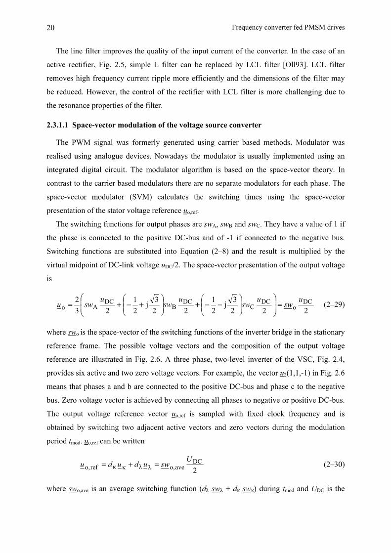
2.3.1.1 Space-vector modulation of the voltage source converter
The PWM signal was formerly generated using carrier based methods. Modulator was
realised using analogue devices. Nowadays the modulator is usually implemented using an
integrated digital circuit. The modulator algorithm is based on the space-vector theory. In
contrast to the carrier based modulators there are no separate modulators for each phase. The
space-vector modulator (SVM) calculates the switching times using the space-vector
presentation of the stator voltage reference uo,ref.
The switching functions for output phases are swA, swB and swC. They have a value of 1 if
the phase is connected to the positive DC-bus and of -1 if connected to the negative bus.
Switching functions are substituted into Equation (2–8) and the result is multiplied by the
virtual midpoint of DC-link voltage uDC/2. The space-vector presentation of the output voltage
is
2223j
21
223j
21
232 DC
oDC
CDC
BDC
Aou
swu
swu
swu
swu =⎟⎟⎠
⎞⎜⎜⎝
⎛⎟⎟⎠
⎞⎜⎜⎝
⎛−−+⎟⎟
⎠
⎞⎜⎜⎝
⎛+−+= (2–29)
where swo is the space-vector of the switching functions of the inverter bridge in the stationary
reference frame. The possible voltage vectors and the composition of the output voltage
reference are illustrated in Fig. 2.6. A three phase, two-level inverter of the VSC, Fig. 2.4,
provides six active and two zero voltage vectors. For example, the vector u2(1,1,-1) in Fig. 2.6
means that phases a and b are connected to the positive DC-bus and phase c to the negative
bus. Zero voltage vector is achieved by connecting all phases to negative or positive DC-bus.
The output voltage reference vector uo,ref is sampled with fixed clock frequency and is
obtained by switching two adjacent active vectors and zero vectors during the modulation
period tmod. uo,ref can be written
2DC
aveo,λλκκrefo,U
swududu =+= (2–30)
where swo,ave is an average switching function (dλ swλ + dκ swκ) during tmod and UDC is the

21
average DC-link voltage. Lead vector uλ is the next active vector in the direction of rotation
and lag vector uκ is the active vector behind uo,ref. Relative durations dλ and dκ of the lead and
lag vectors respectively are
)sin(3
oDC
refo,λ θ
43421m
U
ud = (2–31a)
)3πsin(
3o
DC
refo,κ θ−=
43421m
U
ud (2–31b)
κλ70zero 1 ddddd −−=+= (2–31c)
The coefficient m is called a modulation index. The actual durations are achieved by
multiplying dλ and dκ by tmod. dκ, dλ and zero vectors are taken symmetrically in respect of the
centre of the modulation period, Fig. 2.7. dκ = d1 and dλ = d2. θo is the angle between a voltage
reference vector uref and lag vector, Fig. 2.6. In the literature half of tmod is usually analysed
instead of the full modulation period. In this thesis vector durations are calculated for tmod to
make the equations comparable to those of matrix converters.
IIII
II
IV
V
VI
u1(1,-1,-1)
u2(1,1,-1)u3(-1,1,-1)
u6(1,-1,1)
u4(-1,1,1)
u5(-1,-1,1)
Im
Reu7(1,1,1)u0(-1,-1,-1)
uref
θοdκuκ
dλuλ
1/2
phase a
phase b
-1 1 1 1 1 1 1 -1
-1 -1 -1-11 1 1 1
1 1-1 -1 -1 -1 -1 -1
d0/2 d7/2d1/2 d2/2
1 ( tmod )
phase c
1/2
d7/2 d2/2 d1/2 d0/2
Fig. 2.6 Voltage vectors of VSI. uo,ref is formed in sector I.
Fig. 2.7 Vector placements during one modulating period in the first voltage sector.
If the modulation index m ≤ 1 the amplitude of the voltage reference vector uo,ref equals the
mean output voltage during tmod. The modulation is then said to be linear, meaning |uo,ref| ≤
UDC/ 3 . In this thesis the modulation is performed only in the linear range, 0 ≤ m ≤ 1.
The durations of u7(1,1,1) and u0(-1,-1,-1) and their placements are dependent on the
modulation strategy. In this thesis the placement of the zero vector of the voltage source
inverter (VSI) is symmetrical, Fig. 2.7. Each half modulation period begins and ends at the
zero vector. The active vector is chosen so that the state of switches in only one phase has to

Frequency converter fed PMSM drives
22
be changed during the vector transition. In linear modulation range this method has a
harmonic performance and maximum output voltage rather similar to conventional carrier
based PWM methods with third harmonic injection, [Hol03].
If the VSC is loaded the voltage over DC-link capacitor is the average of the three phase
diode rectifier output: UDC = )/23( π ×ULL,supply (540 V in the case of 400 V supply
network). The maximum output/input voltage ratio of the VSC in the case of linear
modulation is 955.0/3)2/3//()3/( supplyLL,DC ≈= πUU . With active rectifier, Fig. 2.5,
the output voltage is limited by the maximum voltage of the DC-link capacitor and switching
components.
2.3.1.2 Current commutation
In the case of VSI the upper and lower switches of one output phase cannot be conducting
at the same time because the DC-link would be short circuited. This is prevented by a dead
time. During the dead time both switches of the phase are opened and the diodes allow safe
conducting paths for current. The commutation between switches is always forced and the
control of switches requires no information about currents. The commutation is illustrated in
Fig. 2.8, where the active voltage vector of the VSI is changed from vector u1 to u2. The
conducting components are drawn as a straight line.
iAiB
iA
iC
iB iA
iC
vector u1(1,-1,-1) vector u2(1,1,-1)dead time
DC-link
+
-
1. 2. 3.
iB
iC
Fig. 2.8 Current commutation between switches in a voltage source inverter.
2.3.2 Matrix converter
Fig. 2.9a illustrates a conventional 3×3 matrix converter topology [Ven80] where nine bi-
directional switches are implemented using IGBTs. This topology is also called a direct
matrix converter (DMC). The conventional vector modulated DMC, may be replaced by a
vector modulated indirect matrix converter (IMC), which consists of separated line and load
bridges as presented in Fig. 2.9b, [Min93], [Iim97], [Mur01], [Wei01]. This structure is also
called a two-stage matrix converter. In the IMC there are only six active bi-directional
switches instead of nine in the DMC. The load bridge of the IMC is a conventional inverter

23
bridge of a voltage source converter. In theory DMC and IMC have similar properties.
However, the performance of these two topologies is not identical. The differences are
discussed in the following sections.
A B C
a b c
line filter
AC load
a)
A
B
C
a
c
n
p
iDC
b
line filter
line bridge load bridge
AC loadSpa1
Spa2Spb2
Spb1
Spc2
Spc1
uDC
SAp
SAn
b)
Fig. 2.9 a) Direct matrix converter (DMC), b) Indirect matrix converter (IMC).
Every input phase of the matrix converter can be connected to any of the output phases.
Power flow in both directions requires that the switches are bi-directional. Normally, the MC
is fed by a voltage source and, for this reason, the input phases a,b,c should not be short
circuited. If the MC supplies an AC machine which is an inductive load the output phases
A,B,C must never be opened.
In theory nine switches of 3×3 MC have 29 switching states. The aforementioned
constraints limit the possible switching states to 27. The line filter of the MC is usually an LC
circuit. The capacitors provide paths for the currents of the input phases when the phase is not
connected to load. Multistage LC has also been investigated but the simple LC filter is found
to be the best alternative considering cost and size [Whe94].
In the following sections the structure and control of bi-directional switches of MC are
discussed. Current commutation of MC and VSI are compared. A space-vector modulator for
the matrix converter is presented using “fictitious DC-link” method.
2.3.2.1 Bi-directional switches
In this study the bi-directional switch is implemented using IGBTs. Fig. 2.10 illustrates
three switch combinations [Nie96], [Whe02], [Jus05]. Fig. 2.10a shows a common emitter
configuration with a central connection. This switch structure is available as an integrated
IGBT module. The benefit of the integrated structure is the minimised stray inductance.
a) b) c)
Fig. 2.10 Bidirectional switch cells: a) common emitter, b) common collector, c) reverse blocking IGBT.
Frequency converter fed PMSM drives
24
Fig. 2.10b illustrates the common collector configuration. The conduction losses are the
same as for the common emitter configuration. Using the common collector configuration the
number of isolated power supplies can be minimised [Whe02]. Six isolated supplies are
needed if the emitters of three IGBTs connected to each input and output phase are connected
to the same potential. In the case of common emitter switch cell nine isolated supplies are
required. However, if the emitter of three IGBT is connected to the same potential the stray
inductances can cause problems due to the long connections. This is naturally a problem only
if the MC is implemented using discrete components. If the full matrix converter circuit is
integrated into one module the stray inductances are small and the common collector
configuration is a more attractive switch cell structure than the common emitter configuration
[Bru01].
Fig. 2.10c illustrates a switch cell with two reverse blocking IGBTs [Lin01], [Ito04]
connected in antiparallel. This could be the switch cell commonly used in the near future if
reverse blocking IGBTs are further developed.
2.3.2.2 Current commutation
In the MC a short circuit between input phases must be avoided and the output phases
(load phases) must be always connected to some of three input phases. Thus the commutation
must be actively controlled at all times with respect to these basic rules. Each group of three
bi-directional switches connected to each output phase, Fig. 2.9a, is controlled independently
in a such way that the input is not short circuited and the load phases are not opened. This
requires rather complicated commutation strategies compared to VSI.
The commutation is first explained for direct topology (DMC). Commutation techniques
are based on the knowledge of the load current direction [Whe02] or the knowledge of the
voltage over bi-directional switch [Emp98], [Whe04]. An attempt is made to solve the
commutation problem using soft switching techniques but these methods increase the
component count and conduction losses [Whe02]. In this thesis only the load current direction
based commutation methods are discussed.
The first load current direction based method was the four-step commutation [Bur89]. The
four-step commutation from input phase a to input phase b in the case of load phase A is
shown in Fig. 2.11. Similar principles also hold for switches of phases B and C.

25
A
a cbSAa1
SAa2
SAb1
SAb2 SAc2
SAc1
time
SAa1
SAa2
SAb1
SAb2 time
SAa1
SAa2
SAb1
SAb2
i > 0A i < 0A
a) b) c)t1 t2 t3 t4 t1 t2 t3 t4iA
Fig. 2.11 Four-step commutation. a) Switch group of output phase A, b) timing diagram for gate
signals, positive load current, c) timing diagram for gate signals, negative load current.
In Fig. 2.11a the positive current direction is from input (a,b,c) to output A. If iA > 0, Fig.
2.11b, the commutation process begins at the instant t1 when switch SAa2 is turned off. SAa2 is
not conducting. The next step (t2) is to ensure a conducting path for the current from input
phase b) by turning SAb1 on. If ub > ua the current commutates naturally between phases a and
b at this point. If ub < ua the commutation is forced at the instant t3 when SAa2 is turned off.
The last step (t4) is to turn SAb2 on to allow current reversals. Fig. 2.11c shows the timing
diagram in the case of negative iA. The delays between the switching instants are dependent
on the characteristics of the semiconductor devices used in the bi-directional switches.
The four-step commutation can be reduced to three-step if t2 = t3. SAa1 is turned off at the
same instant as SAb1 is turned on. This method requires that the turn-off delay of the switch
device is longer than the turn-on delay [Whe04]. In the opposite case the conduction path
opens and an overvoltage occurs. In the two-step strategy [Swe91], [Emp98] only the
conducting component of the bi-directional switch is turned on. Thus no switching at instants
t1 and t4 is performed. One-step strategy is similar to two-step but there is no delay between
the switching of SAa1 and SAb1. Similar to three step strategy, this requires the turn-off time to
be longer than the turn-on time. In this thesis the four-step commutation is applied.
Indirect matrix converter
The indirect matrix converter, Fig. 2.9b, can be considered as a 3×2 matrix converter and
voltage source inverter connected in series. The output voltage between two phases of the line
bridge (3×2 DMC) is controlled to be a DC voltage. Thus the voltage between the two outputs
can be considered as a DC-link even if there is no energy storage. IMC produces a three phase
output voltage from DC-link similar to VSI. The commutation of the line bridge of the IMC is
performed using similar principles as explained for the DMC. The difference is that the input
phases a,b,c are not connected to the load phases directly but to the two DC-buses. The
commutation of the VSI was explained above and it is similar to the commutation of the load

Frequency converter fed PMSM drives
26
bridge of the IMC.
2.3.2.3 Space-vector modulation of the matrix converter
Several modulation strategies have been proposed for the matrix converter. The most
important methods are discussed and references given in [Whe02]. In this thesis only the
space-vector modulation [Hub89], [Hub95], [Nie96], [Cas02], [Jus05] is discussed.
The direct matrix converter (DMC) has 27 allowed switching states [Hub95]. The allowed
states can be classified into three groups [Whe02].
Group I: Each output phase A,B,C is connected to a different input phase a,b,c. These
vectors rotate at the frequency of the supply network and have a constant amplitude.
Group II: Two output phases are connected to a common input line and the remaining one
is connected to one of the other input lines. These space-vectors have a fixed direction but
varying amplitude.
Group III: All output phases are connected to the same input phase. The output vectors
have zero amplitude.
In the SVM method discussed in this study the Group I vectors are not used. The desired
output voltage is synthesized from Group II active vectors and Group III zero vectors.
The SVM is also called an indirect modulation method because it is often derived using
ideal IMC topology, Fig. 2.12, with “fictitious DC-link”. This is possible if the vectors of
A
B
C
a
c
n
p
i
bu DC
DC
Spa
Sna
Spb Spc
Snb Snc SAn SBn SCn
SAp SBp SCp
Fig. 2.12 Ideal IMC used in the space-vector modulation analysis.
Group I are not used. The line and load bridges are analysed separately and finally the results
are combined. The input voltages and voltage references of the load are assumed to be
constant during one modulation period.
Line bridge
Let us first define switching functions swa, swb, swc for each input phase. They can have
values –1, 0 and 1. swa = 0 means that the input phase a is not connected to DC-bus. swa = 1
means that the phase a is connected to bus p, which means the ideal switch Spa, Fig. 2.12, is

27
conducting. If swa = -1 the Sna is conducting. The same principles also hold for phases b and c.
To prevent the short circuit only one input phase can be connected to each bus. Thus
swa+ swb + swc = 0 (2–32)
The phase currents are: ia = swaiDC, ib = swbiDC, ic = swciDC. Using (2–8) the space-vector of the
input current in stationary reference frame is
DCiDCcDCbDCai 23j
21
23j
21)3/2( iswiswiswiswi =⎟
⎟⎠
⎞⎜⎜⎝
⎛⎟⎟⎠
⎞⎜⎜⎝
⎛−−+⎟⎟
⎠
⎞⎜⎜⎝
⎛+−+= (2–33)
The combinations allowed by (2–32) are illustrated in Fig. 2.13 for positive and negative iDC.
For example i1(1,0,-1) means swa = 1, swb = 0, swc = -1.
a)
θi
b)
dγ
dδ iδ
iδ
iγ
iγ
ii,refI
III II
IV
V VI
0
i2(0,1,-1)
i6(1,-1,0)
i3(-1,1,0)
i5(0,-1,1)
i1(1,0,-1)
i4(-1,0,1)
c)
I
IIIII
IV
VVI
0
ix(swa,swb,swc)
i5(0,-1,1)
i3(-1,1,0)
i6(1,-1,0)
i2(0,1,-1)
i4(-1,0,1)
i1(1,0,-1)
Im
Re Re
Im
iDC > 0 iDC < 0
Fig. 2.13 Input current sectors and allowed switching state vectors for a) iDC > 0, b) iDC < 0, c) composition of the current vector in sector I.
The current reference vector ii,ref is sampled with fixed clock frequency and is obtained by
switching two adjacent active vectors during the modulation period tmod, Fig. 2.13c. Thus the
main principle is similar compared to the composition of the voltage vector in the case of
VSC, Fig. 2.6. The input current vector during tmod, Fig. 2.13c, can be written
δδγγrefi, ididi += (2–34)
where ( )iDC
refi,δi
DC
refi,γ sin,
3sin θθ
i
idπ
i
id =⎟
⎠⎞
⎜⎝⎛ −=
dγ and dδ are relative on-durations for active current vectors. γ and δ denote lag and lead
vector respectively.
If the line bridge is ideal the DC-link power is (3/2)Reu ii i*= uDCiDC [Vas92]. ui is the
space-vector representing the three-phase input voltage. The input current vector from (2–33)

Frequency converter fed PMSM drives
28
is substituted into the expression of the DC-link power and both sides are divided by iDC. The
instantaneous DC-link voltage can be written as
*iiDC Re
23 swuu = (2–35)
The average of the switching function vector swi during a modulation period tmod is the sum of
two vectors, Fig. 2.13c, swi,ave = dγswi,γ + dδswi,δ. The average DC-link voltage during tmod can
be written
( )*δi,iδ
*γi,iγ
*avei,iDC ReRe
23Re
23 swudswudswuU +== (2–36)
Load bridge
The load bridge in Fig. 2.12 is the same circuit as the VSI. Therefore Equations (2–30)-(2–
31) also hold for the load bridge of the IMC. In this thesis the zero vector placement of the
MC is not the same as that used with VSI, Fig. 2.7. The switching strategy of the MC is
explained later in this section. The active output voltage vectors of the IMC and the
composition of uo,ref are presented in Fig. 2.14.
IIII
II
IV
V
VI
0
ux(swA,swB,swC)
uo,ref
uλ
dκuκ
dλuλ
θo
(a)
(b)
uκ
u1(1,-1,-1)
u2(1,1,-1)u3(-1,1,-1)
u6(1,-1,1)
u4(-1,1,1)
u5(-1,-1,1)
Im
Re
Fig. 2.14 a) Output voltage vectors, b) composition of the output voltage in sector I.
Synthesis of the line and load bridges
The space-vector modulation of the MC is achieved by combining the equations of the line
and load bridges [Hub95]. During tmod the reference voltage vector uo,ref (2–30) is composed
of two active vectors, Fig. 2.14. Similarly the average output switching function during tmod is:
swo,ave = dκswκ + dλswλ. When swo is replaced by swo,ave in (2–29) and the expression of UDC
(2–36) is substituted into (2–29) the average output voltage during tmod can be written

29
( ) (
)*δiλδλ
*γiλγλ
*δiκδκ
*γiκγκ
*δiδ
*γiγaveo,aveo,
Re
ReReRe43
ReRe43
swuswdd
swuswddswuswddswuswdd
swudswudswu
+
++=
+=
(2–37)
If the load bridge is ideal uo,ave = uo,ref. Now the direct relation between output and input
voltage is obtained. It can be seen from (2–37) that the output voltage is composed using four
active voltage vectors. There are two DC voltage levels, (3/4)Reuiswγ* and (3/4)Reuiswδ
*.
The output voltage is obtained using both of them with load bridge states swκ and swλ. The
relative on-durations of the active vectors are
( ) ( )( ) ( )
( ) ( )( ) ( )ioδλλδ
ioγλλγ
ioκκ
ioγκκγ
sinsin
3/sinsinsin3/πsin
3/πsin3/πsin
θθθπθθθ
θθ
δδ
mddd
mdddmddd
mddd
==
−==−==
−−==
(2–38)
The time reserved for zero vectors is
δδ κλγκκγ0 1 ddddd −−−−= (2–39)
Maximum output voltage
The maximum output voltage of the MC can be calculated using (2–36). Fundamental
frequency components of the input voltage and the average switching function swi,ave are used.
ω1t is the angle of the fundamental frequency input voltage vector ui,1. The angle of the
fundamental frequency input current ii,1 and average switching function swi,ave is then
ω1t - ϕ i ,1 where ϕ i , 1 is the fundamental displacement angle of the input. The average DC-link
voltage during tmod is
⎭⎬⎫
⎩⎨⎧= +− 1,i1
avei,1
1,DC Re23 ϕωω tjtj
i esweuU (2–40)
|swi,ave| denotes current ratio |ii,1|/iDC which cannot have values greater than unity. Thus the
average DC-link voltage during tmod in the case of unity (|ii,1|/iDC) is
)cos(23
i,11,iDC ϕuU = (2–41)
The maximum value of the modulation index (m = 3 |uo,ref|/UDC) of the load bridge is unity
in linear modulation (see Section 2.3.1.1). If (2–41) is substituted into the equation of the
Frequency converter fed PMSM drives
30
duration of the active output vector of the VSI (2–31) the modulation index m can be written:
1,ii,1
refo,
cos3
2
ϕu
um = (2–42)
Thus the maximum theoretical output/input voltage ratio in the case of linear modulation is
866.02/3 ≈ (m = 1) and is achieved when the displacement power factor of the input is
unity. In this thesis cosϕ i ,1 = 1. In the case of VSC with diode rectifier the maximum
output/input voltage ratio is approximately 0.95 [Hol03].
Switching strategy
In this study the switching states during one modulation period are arranged applying the
following principles [Jus05], [Nie96]:
1. Only one output phase changes its state when the switching state vector is changed.
2. Active vectors are taken symmetrically in respect of the centre of the modulation period.
3. Zero vector is taken in the middle of the modulation period.
This strategy gives small switching losses. [Cha03] has presented a strategy where the losses
are further reduced.
Now the zero vector is not divided as was the case with VSC, Fig. 2.7. The strategy is
clarified in Table 1. Examples of four current and voltage sector combinations are presented.
Let us consider the case when the input current vector and the output voltage vector are in
sector I. It can be seen in Fig. 2.13 and Fig. 2.14 that the state swκγ connects output phase A to
input phase a. B and C are connected to b. This state is denoted abb (state 1 in Table 1). State
swλγ gives aab and so on. This is illustrated in Fig. 2.15. It is important to note that if the sum
of the current and voltage sectors is an odd number, the order of load bridge switching states
is changed. The output zero vector requires no changes in switches of the fictitious line bridge
because the conducting path of the input current is opened anyway when all output phases are
connected to the same bus, Fig. 2.15.
In [Apa03], [Cas02] the zero vector of MC is divided into three parts. In that case every
tmod/2 period begins and ends with zero vector. This method was already explained in the case
of VSI in Section 2.3.1. This strategy decreases the high frequency harmonics in the input and
low frequency harmonics in the output [Apa03]. It also increases the switching losses
compared to zero vector placement of Table 1 because the number of switching events is
increased.

31
Table 1. Switching states and on-durations in four cases during one modulation period.
usec isec state 1 state 2 state 3 state 4 state 5 state 6 state 7 state 8 state 9 I I abb aab aac acc ccc acc aac aab abb I II aac acc bcc bbc bbb bbc bcc acc aac II I bab aab aac cac ccc cac aac aab bab II III cbc bbc bba aba aaa aba bba bbc cbc durations tγ(κ,λ)/2 tγ(λ,κ)/2 tδ(λ,κ)/2 tδ(κ,λ)/2 t0 tδ(κ,λ)/2 tδ(λ,κ)/2 tγ(λ,κ)/2 tγ(κ,λ)/2
Input vector swγ swδ swγ Output vector: odd (usec + isec)
swλ swκ swλ 0 swλ swκ swλ
Combined state swλγ swκγ swκδ swλδ 0 swλδ swκδ swκγ swλγ Output vector:
even (usec + isec) swκ swλ swκ 0 swκ swλ swκ
Combined state swκγ swλγ swλδ swκδ 0 swκδ swλδ swλγ swκγ tmod/2 tmod/2
abc
ABC
swκγ
abb
swλγ
aab
abc
ABC
swλδ
aac
abc
ABC
abc
ABC
swκδ
acc
abc
ABC
0
ccc
γ κ γ λ δ λ
δ κ 0δ
Fig. 2.15 Switching states of MC during tmod/2. usec = I and isec = I (Table 1).
Indirect matrix converter
The analysis presented above was for the DMC topology, Fig. 2.9a. The line and load
bridges are fictitious for DMC but real circuits in the case of IMC, Fig. 2.9b. If the switches
are ideal both topologies have similar performance. In practice the losses and output
waveforms of DMC and IMC are not identical. The on-state losses of the IMC are higher
because there are more components in the current path, Fig. 2.9. In DMC the output voltage is
composed by switching the sinusoidal line-to-line supply voltages. In IMC the output voltage
is formed from DC-link voltage which has a PWM waveform. In the case of the IMC the zero
vector is formed by connecting all the load phases to the upper or lower DC bus. During the
zero vector the input current vector is active (2–33) but iDC is zero because the output phases
are connected to the same bus, Fig. 2.15.

Frequency converter fed PMSM drives
32
2.4 Comparison of non-ideal properties of VSC and MC
In the ideal case the voltage reference vector uo,ref equals the mean output voltage produced
during each modulation period. This requires linear modulation range and ideal components
in the main circuit. In practice the voltage drop over semiconductors causes power losses and
distorts the output waveform of the converter. The necessary switching strategies (dead times
and overlapping times) to prevent short circuits and overvoltages are the other source of
distortion. In this section these non-ideal properties of the voltage source converters and
matrix converters are compared.
In many sensorless control methods the motor input voltage should be known as accurately
as possible. The PWM voltage is not usually measured because the number of sensors would
be increased and the sampling rate is limited. Therefore the estimator algorithms use the
voltage reference vector as the output voltage information. The differences between uo,ref and
the true output voltage in the VSCs and MCs are studied in this section. Power losses are
briefly discussed.
Modelling of the non-linear properties of the voltage source inverter bridge has been
widely studied in the literature [Hol02], [Mun99], [Hol02]. Therefore only the basic
principles are presented here. The non-linear properties of DMC have been studied in
[Lee04b] but IMC has not been analysed earlier. Jussila and the author have compared the
non-linear properties of DMC and IMC using a vector form in [Jus06].
2.4.1 Non-linear model of the bi-directional switch
Fig. 2.16 shows the forward characteristics of SKM75GA123D IGBT module. This
module is used in the DMC prototype (Appendix B) and in the line bridge of the IMC
prototype. In the analysis of the non-linear properties of the VSI and MC, diodes and IGBTs
are linearized using a constant threshold voltage Uth and constant resistance rd, Fig. 2.16. In
the literature [Mun99], [Hol02] the average value of the IGBT and the diode Uth and rd are
used. Therefore only one value for Uth and rd is needed. This simplification is also done in this
thesis.
In the DMC and in the line bridge of the IMC the bi-directional switches contain an IGBT
and a diode connected in series. Therefore Uth and rd are threshold voltages and resistances for
two devices connected in series. In the load bridge of the IMC and in the VSI Uth and rd are
for one device. To avoid confusion between MC topologies Uth and rd are denoted as Uth,i, rd,i
in the line bridge of the IMC. The load bridge quantities of the IMC are marked Uth,o, rd,o.

33
In this study the 5 kVA prototype MCs feed a 3.5 kW PMSM, Appendix A. Due to the low
power level the operating area is in the non-linear part of the Fig. 2.16. The selection of Uth
and rd for the simulation model is therefore rather difficult.
UCE (V)0 1 2 3 4
IC (A)
20
40
80
60
IGBT
diode
operating area
Uth
rd
125 C
Fig. 2.16 Forward characteristics of the power devices in SKM75GA123D module.
2.4.2 Non-linear model of the VSI
Fig. 2.17a illustrates the control of phase A of the VSI. A short circuit is avoided using a
delay td called dead time. The block td in Fig. 2.17a delays the rising edges of the signals
controlling the switches SAp and SAn.
The gate signal, on and off durations of the switches of phase A, are shown in Fig. 2.17b
during one modulation period. The voltage between the output and fictitious central point 0 of
the DC-link is also shown in the case of negative and positive current directions. Ud and UI
denote an on-state voltage drop over diode and IGBT respectively. Let us consider the case iA
< 0. In the beginning SAn conducts iA to bus n. During the first half of tmod SAn is turned off
and after dead time td SAp is turned on. The output A is connected to negative bus via SAn until
the current is commutated from SAn to diode dp. The commutation is complete after the turn
off delay toff. When phase A is connected to the negative bus via SAn the voltage UA0 = -UDC/2
+ UI. When iA flows to a positive bus through dp: UA0 = UDC/2 + Ud. The next transition
begins when swa changes its state from 1 to -1. dp conducts until the dead time and the turn-on
delay ton of SAn are over. Finally the output A is again connected to a negative bus via San. The
rate of change of the voltage over the semiconductors is assumed to be infinite.
It can be seen in Fig. 2.17b that with a negative current the area above the zero voltage
level is increased compared to the desired voltage pulse UA0,ref. For positive current the area is
decreased by the same amount. In the analysis the average on-state voltage drop (Ud + UI)/2 is
used [Hol02] and is denoted Uon = Uth + rdi. The difference between Ud and UI is assumed to
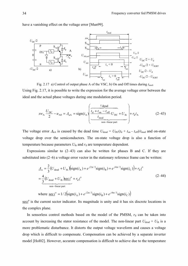
Frequency converter fed PMSM drives
34
have a vanishing effect on the voltage error [Mun99].
Α
p
td
td
swa
SAp
SAniA
0
a)
+−
swa
SAptd tdSAn
UA0,ref
UA0
toffiA < 0
ton
UA0 iA > 0ton toff
tmod
b)
dp
dnUDC/2 + Ud
-UDC/2 + UIGBT
UDC/2
-UDC/2 n
UDC/2 - Ud
-UDC/2 - UIGBT
UDC/2
-UDC/2
Fig. 2.17 a) Control of output phase A of the VSC, b) On and Off times during tmod.
Using Fig. 2.17, it is possible to write the expression for the average voltage error between the
ideal and the actual phase voltages during one modulation period.
Ad
partlinearnon
thDCmod
offondAuAA0
DCA
dead
)(sign2
irUUt
ttti∆u
Usw
U
+⎟⎟⎟⎟
⎠
⎞
⎜⎜⎜⎜
⎝
⎛
+−+
==−
−4444 34444 21
444 8444 76
(2–43)
The voltage error ∆uA is caused by the dead time Udead = UDC(td + ton - toff)/tmod and on-state
voltage drop over the semiconductors. The on-state voltage drop is also a function of
temperature because parameters Uth and rd are temperature dependent.
Expressions similar to (2–43) can also be written for phases B and C. If they are
substituted into (2–6) a voltage error vector in the stationary reference frame can be written:
( )( )( ) s
d
partlinearnon
sthdead
sdC
3/π4B
3/π2Athdeadu
sec34
)(sign)(sign)(sign32
iriUU
irieieiUU∆ jj
++=
++++=
−444 3444 21
(2–44)
where ( ))(sign)(sign)(sign2/1sec C3/π4
B3/π2
As ieieii jj ++=
secis is the current sector indicator. Its magnitude is unity and it has six discrete locations in
the complex plane.
In sensorless control methods based on the model of the PMSM, rd can be taken into
account by increasing the stator resistance of the model. The non-linear part Udead + Uth is a
more problematic disturbance. It distorts the output voltage waveform and causes a voltage
drop which is difficult to compensate. Compensation can be achieved by a separate inverter
model [Hol02]. However, accurate compensation is difficult to achieve due to the temperature

35
dependency and non-linear nature of semiconductors, Fig. 2.16.
Fig. 2.18 illustrates the effect of the non-linear properties of the VSI. The resistive voltage
drop is omitted. Fig. 2.18a shows the voltage drop in one phase (2–43). The real and
imaginary parts of the non-linear voltage vector in the stationary reference frame and the
length of the vector are shown in Fig. 2.18b, c. In the simulations of Fig. 2.18 (td+ton-toff)/tmod
= 0.003, Uth = 0.3 V and UDC = 540 V.
a) b) c)
Fig. 2.18 a) Voltage components in one phase caused by the Udead and Uth. b) Components of the non-linear voltage vector in stationary reference frame. c) Length of the voltage vector.
2.4.3 Non-linear model of the IMC
In the VSI the source voltage for the load is the DC-link voltage. In the matrix converter
the source voltages are the line-to-line voltages of the supply network. In the case of the IMC
the voltage errors of the line and load bridges are discussed separately.
2.4.3.1 Line bridge
The commutation of the current in the line bridge of the IMC is illustrated in Fig. 2.19. Fig.
2.19a shows the four-step commutation in the switch group of bus p between phases a and b
in the input current sector 2, Fig. 2.13, in the case of positive current direction in the DC-link.
The positive current direction is from the line side to the load, Fig. 2.12. Fig. 2.19b shows the
same with a negative iDC. In sector 2 the bus n is connected to the phase c and the positive bus
p is connected either to phase a or b. The switches Spa1, Spa2, Spb1, Spb2 of the input phases were
illustrated in Fig. 2.9b.
As discussed earlier, the commutation is forced or natural depending on the values of
phase voltages taking part in the process. During one modulation period one commutation is
natural and the other is forced. If the commutation is forced the connection of bus p and the
new phase is delayed by the overlapping time tc plus the turn-off delay toff. In natural
commutation the current transfers to the new phase after turn-on delay ton. In Fig. 2.19 the on-
state voltage drop of the bi-directional switch is denoted as Uon and consists of the threshold

Frequency converter fed PMSM drives
36
voltage Uth,i and resistive voltage drop rd,iiDC.
Spa1
Spa2
Spb1
Spb2
ua > ub:
ua < ub:
up
up tc
ton
tc
tontoff
toff
tSbp
ua-Uon
ua-Uon
ub-Uon
iDC > 0
Spa1
Spa2
Spb1
Spb2
ua > ub:
ua < ub:
up
up
tc
tc
tontoff
ua+Uon
ua+Uon
ub+Uon
iDC < 0
toff ton
a)
b)
ua
ub ideal commutationup
Fig. 2.19 Four-step commutation in switch group of bus p between phases a and b in current sector 2. a) iDC flows in a positive direction, b) iDC flows in a negative direction. tSbp denotes the desired
time when bus p is connected to phase b.
The average voltage error during one modulation period between the ideal and real DC-link
voltage can be defined by subtracting the voltage with losses and delays from ideal p bus
voltage up, Fig. 2.19, given in (2–36). The average voltage used in the generation of the active
output voltage vectors during one modulation period is [Jus06]
( ) ui*iδδδ
*iγγγui
*avei,iDC ReRe
23Re
23 ∆swudswud∆swuU −+=−= (2–45)
where ⎟⎟⎠
⎞⎜⎜⎝
⎛+−−+−= )()sign( DCid,ith,medLL,
mod
onoffcDCui irUu
tttti∆ (2–46)
∆ui is the voltage component produced by the non-ideal line bridge. uLL,med is the is the line-to-
line voltage with the middlemost amplitude. In current sector 2 the commutation occurs
between phases a and b, Fig. 2.13 (cosϕ i = 1). Therefore the voltage error is dependent on the
amplitude of the line-to-line voltage uab which is uLL,med in sector 2. In the other sectors the
voltage error is similarly dependent on uLL,med. The voltage component ∆ui during one

37
fundamental period of the input voltage is illustrated in Fig. 2.20. fin is the frequency of the
supply network. The DC-link voltage contains the multiples of the sixth harmonics of the
supply frequency. The amplitudes of these harmonics are small compared to the average uDC
(2–40).
UDC,ideal (2-36)
UDC
-sign(iDC)(Uth,di+ rdi|iDC|)uLL,med,(peak) (tc+toff-ton) tmod
1/fin
uLL,med,(peak) = ULL,RMS / 2
Fig. 2.20 UDC,ref of the IMC and the actual UDC (2-45). iDC flows to positive direction.
It can be seen in (2–46) that the overlapping time boosts the DC-link voltage if iDC > 0. It is
also easy to see in Fig. 2.19 where the bus p is connected to a higher input voltage longer than
the desired time tSbp. Overlapping has an opposite effect compared to dead time (2–43). iDC is
positive when the displacement power angle of the load is between -π/6 and π/6 [Kol02].
2.4.3.2 Load bridge
The load bridge of the IMC is similar to the VSI. However, the control of the switches of
the load bridge is not similar in this thesis. In the case of the VSI every phase is switched
twice during tmod, Fig. 2.7. In the case of IMC one output phase is switched twice, one four
times and one is not switched during one modulation period. The number of state transitions
of the switch depends the sector of the output voltage [Jus06]. It can be seen in Table 1 and in
Fig. 2.15 that the output phase C is not switched during one modulation period if the output
voltage reference is in sector 1. Therefore the voltage error in one phase caused by the dead
time is a function of the sign of the current and also a function of the sector of the voltage
reference uo,ref, Table 2. In Table 2 Udead is the voltage error in the case of two switchings
during tmod: Udead = sign(iphase)UDC(td + ton – toff)/tmod (2–43).
Table 2. Dead time effect of the load bridge of the IMC.
Sector of uo,ref UdA( ×Udead) UdB( ×Udead) UdC ( ×Udead)
1 1 2 0 2 2 1 0 3 0 1 2 4 0 2 1 5 2 0 1 6 1 0 2
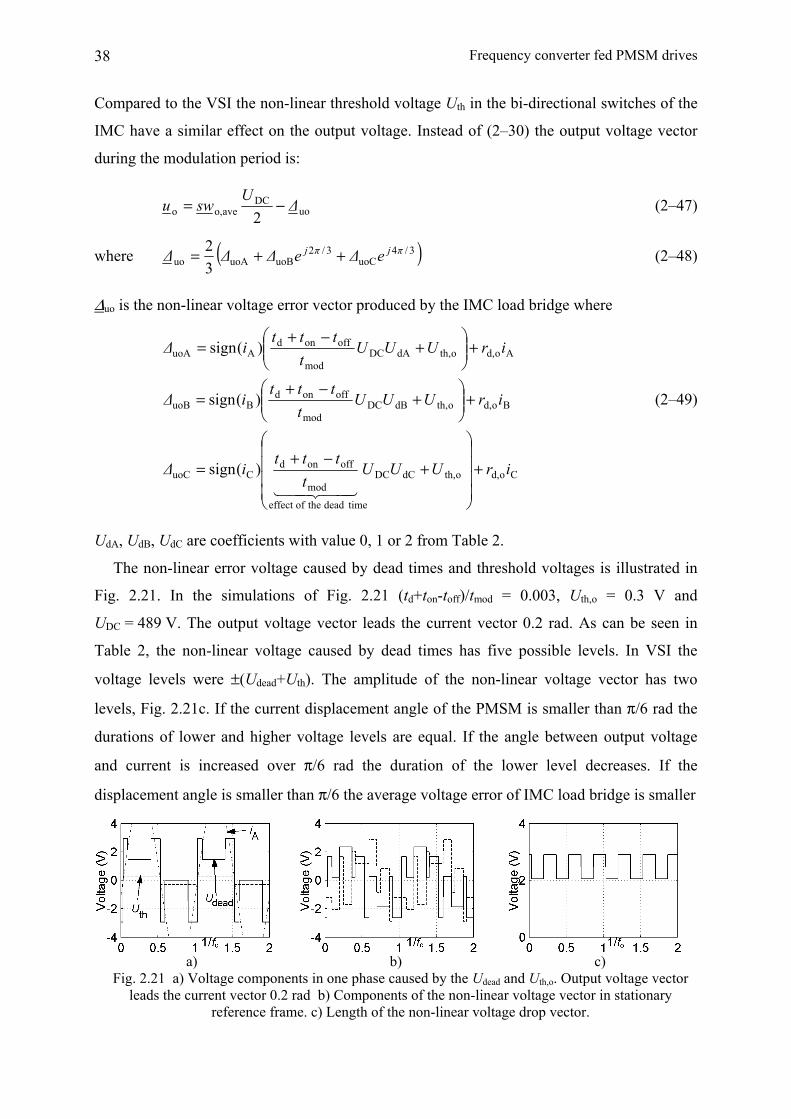
Frequency converter fed PMSM drives
38
Compared to the VSI the non-linear threshold voltage Uth in the bi-directional switches of the
IMC have a similar effect on the output voltage. Instead of (2–30) the output voltage vector
during the modulation period is:
uoDC
aveo,o 2∆
Uswu −= (2–47)
where ( )3/4uoC
3/2uoBuoAuo 3
2 πjπj e∆e∆∆∆ ++= (2–48)
∆uo is the non-linear voltage error vector produced by the IMC load bridge where
Cod,oth,dCDC
time dead theofeffect
mod
offondCuoC
Bod,oth,dBDCmod
offondBuoB
Aod,oth,dADCmod
offondAuoA
)(sign
)(sign
)(sign
irUUUt
ttti∆
irUUUt
ttti∆
irUUUt
ttti∆
+⎟⎟⎟⎟
⎠
⎞
⎜⎜⎜⎜
⎝
⎛
+−+
=
+⎟⎟⎠
⎞⎜⎜⎝
⎛+
−+=
+⎟⎟⎠
⎞⎜⎜⎝
⎛+
−+=
4434421
(2–49)
UdA, UdB, UdC are coefficients with value 0, 1 or 2 from Table 2.
The non-linear error voltage caused by dead times and threshold voltages is illustrated in
Fig. 2.21. In the simulations of Fig. 2.21 (td+ton-toff)/tmod = 0.003, Uth,o = 0.3 V and
UDC = 489 V. The output voltage vector leads the current vector 0.2 rad. As can be seen in
Table 2, the non-linear voltage caused by dead times has five possible levels. In VSI the
voltage levels were ±(Udead+Uth). The amplitude of the non-linear voltage vector has two
levels, Fig. 2.21c. If the current displacement angle of the PMSM is smaller than π/6 rad the
durations of lower and higher voltage levels are equal. If the angle between output voltage
and current is increased over π/6 rad the duration of the lower level decreases. If the
displacement angle is smaller than π/6 the average voltage error of IMC load bridge is smaller
a) b) c)
Fig. 2.21 a) Voltage components in one phase caused by the Udead and Uth,o. Output voltage vector leads the current vector 0.2 rad b) Components of the non-linear voltage vector in stationary
reference frame. c) Length of the non-linear voltage drop vector.

39
compared to VSI due to the smaller DC-link voltage.
2.4.4 Non-linear model of the DMC
During every modulation period two output phases of the DMC change their state twice
and one four times, Table 1. The sector of the output voltage reference determines the phase
switched four times [Jus06]. As explained in Section 2.3.2.2 the commutation principle of the
DMC and the line bridge of the IMC is similar. Thus the voltage error of one phase caused by
one forced and one natural commutation during tmod has the form uLL(tc + toff - ton)/tmod, also in
the case of DMC. uLL is the line-to-line input voltage taking part in the forming of the output
phase voltage. As discussed in Section 2.4.3.1 the overlapping time tc increases the output
voltage (2–46), Fig. 2.19. This also holds for the output voltage of the DMC.
Let us assume that uo,ref and ii,ref both lie in their sector 1. It can be seen in Table 1 and Fig.
2.15 that phase A is formed from the input phases a and c. C is formed using b and c. The
input phase connected to A and C is changed twice during tmod. The input phase connected to
the output B is changed four times during tmod. uB is formed using line-to-line voltages uab and
uca. When the current and voltage references are in sector 1, uab is the highest of the line-to-
line voltages. uca is the lowest one and ubc is the middlemost. The same principle also holds
for other current-voltage sector combinations, Table 3. The voltage error in one phase caused
by the non-linear properties of the DMC topology is dependent on the highest uLL, the lowest
uLL, the middlemost uLL or the voltage (highest uLL - lowest uLL).
Table 3. Line-to-line input voltages determining the non-linear voltage error of the DMC.
Sector of uo,ref Sector of ii,ref Phase A Phase B Phase C Odd |uLL,min| uLL,max- uLL,min |uLL,med| 1 Even |uLL,med| uLL,max- uLL,min uLL,max Odd uLL,max- uLL,min |uLL,min| |uLL,med| 2 Even uLL,max- uLL,min uLL,med uLL,max Odd |uLL,med| |uLL,min| uLL,max- uLL,min 3 Even uLL,max |uLL,med| uLL,max- uLL,min Odd |uLL,med| uLL,max- uLL,min uLL,min 4 Even uLL,max uLL,max- uLL,min |uLL,med| Odd uLL,max- uLL,min |uLL,med| |uLL,min| 5 Even uLL,max- uLL,min uLL,max |uLL,med| Odd |uLL,min| |uLL,med| uLL,max- uLL,min 6 Even |uLL,med| uLL,max uLL,max- uLL,min
Using the equation of the ideal output voltage of the VSI (2–29) and the equation of the
fictitious DC-link voltage (2–36) the output voltage vector of the DMC can be written
u*
avei,ioo Re43 ∆swuswu −= (2–50)
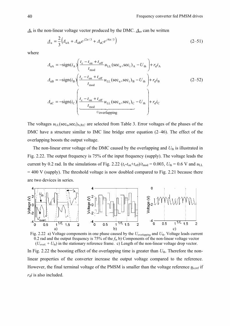
Frequency converter fed PMSM drives
40
∆u is the non-linear voltage vector produced by the DMC. ∆uo can be written
( )3/4uC
3/2uBuAu 3
2 πjπj e∆e∆∆∆ ++= (2–51)
where
CdthCiuLLmod
offoncCuC
BdthBiuLLmod
offoncBuB
AdthAiuLLmod
offoncAuA
goverlappin
)sec,(sec)(sign
)sec,(sec)(sign
)sec,(sec)(sign
irUut
ttti∆
irUut
ttti∆
irUut
ttti∆
U
+
⎟⎟⎟⎟⎟
⎠
⎞
⎜⎜⎜⎜⎜
⎝
⎛
−+−
−=
+⎟⎟⎠
⎞⎜⎜⎝
⎛−
+−−=
+⎟⎟⎠
⎞⎜⎜⎝
⎛−
+−−=
44444 344444 21
(2–52)
The voltages uLL(secu,seci)A,B,C are selected from Table 3. Error voltages of the phases of the
DMC have a structure similar to IMC line bridge error equation (2–46). The effect of the
overlapping boosts the output voltage.
The non-linear error voltage of the DMC caused by the overlapping and Uth is illustrated in
Fig. 2.22. The output frequency is 75% of the input frequency (supply). The voltage leads the
current by 0.2 rad. In the simulations of Fig. 2.22 (tc-ton+toff)/tmod = 0.003, Uth = 0.6 V and uLL
= 400 V (supply). The threshold voltage is now doubled compared to Fig. 2.21 because there
are two devices in series.
a) b) c)
Fig. 2.22 a) Voltage components in one phase caused by the Uoverlapping and Uth. Voltage leads current 0.2 rad and the output frequency is 75% of the fin b) Components of the non-linear voltage vector (Uoverl. + Uth) in the stationary reference frame. c) Length of the non-linear voltage drop vector.
In Fig. 2.22 the boosting effect of the overlapping time is greater than Uth. Therefore the non-
linear properties of the converter increase the output voltage compared to the reference.
However, the final terminal voltage of the PMSM is smaller than the voltage reference uo,ref if
rdi is also included.
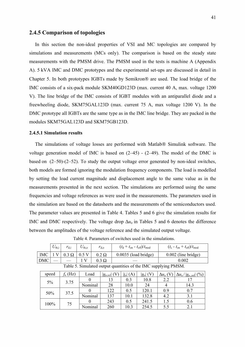
41
2.4.5 Comparison of topologies
In this section the non-ideal properties of VSI and MC topologies are compared by
simulations and measurements (MCs only). The comparison is based on the steady state
measurements with the PMSM drive. The PMSM used in the tests is machine A (Appendix
A). 5 kVA IMC and DMC prototypes and the experimental set-ups are discussed in detail in
Chapter 5. In both prototypes IGBTs made by Semikron® are used. The load bridge of the
IMC consists of a six-pack module SKM40GD123D (max. current 40 A, max. voltage 1200
V). The line bridge of the IMC consists of IGBT modules with an antiparallel diode and a
freewheeling diode, SKM75GAL123D (max. current 75 A, max voltage 1200 V). In the
DMC prototype all IGBTs are the same type as in the IMC line bridge. They are packed in the
modules SKM75GAL123D and SKM75GB123D.
2.4.5.1 Simulation results
The simulations of voltage losses are performed with Matlab® Simulink software. The
voltage generation model of IMC is based on (2–45) - (2–49). The model of the DMC is
based on (2–50)-(2–52). To study the output voltage error generated by non-ideal switches,
both models are formed ignoring the modulation frequency components. The load is modelled
by setting the load current magnitude and displacement angle to the same value as in the
measurements presented in the next section. The simulations are performed using the same
frequencies and voltage references as were used in the measurements. The parameters used in
the simulation are based on the datasheets and the measurements of the semiconductors used.
The parameter values are presented in Table 4. Tables 5 and 6 give the simulation results for
IMC and DMC respectively. The voltage drop ∆uo in Tables 5 and 6 denotes the difference
between the amplitudes of the voltage reference and the simulated output voltage.
Table 4. Parameters of switches used in the simulations.
Uth,i rd,i Uth,o rd,o (td + ton - toff)/tmod (tc - ton + toff)/tmod
IMC 1 V 0.3 Ω 0.5 V 0.2 Ω 0.0035 (load bridge) 0.002 (line bridge) DMC — — 1 V 0.3 Ω — 0.002
Table 5. Simulated output quantities of the IMC supplying PMSM.
speed fo (Hz) Load |uo,ref| (V) |io| (A) |uo| (V) ∆uo (V) ∆uo / |uo,,ref| (%)0 13 0.3 10.8 2.2 17 5% 3.75 Nominal 28 10.0 24 4 14.3 0 122 0.5 120.1 0.9 0.7 50% 37.5 Nominal 137 10.1 132.8 4.2 3.1 0 243 0.5 241.5 1.5 0.6 100% 75 Nominal 260 10.3 254.5 5.5 2.1
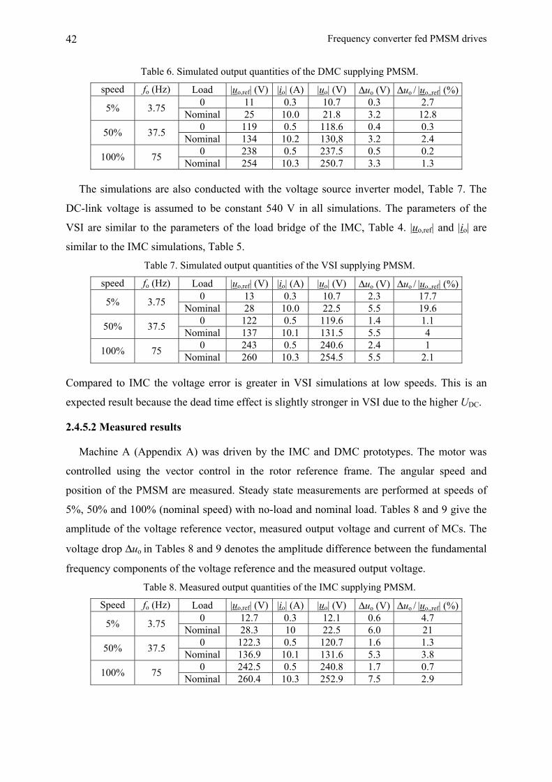
Frequency converter fed PMSM drives
42
Table 6. Simulated output quantities of the DMC supplying PMSM.
speed fo (Hz) Load |uo,ref| (V) |io| (A) |uo| (V) ∆uo (V) ∆uo / |uo,,ref| (%)0 11 0.3 10.7 0.3 2.7 5% 3.75 Nominal 25 10.0 21.8 3.2 12.8 0 119 0.5 118.6 0.4 0.3 50% 37.5 Nominal 134 10.2 130,8 3.2 2.4 0 238 0.5 237.5 0.5 0.2 100% 75 Nominal 254 10.3 250.7 3.3 1.3
The simulations are also conducted with the voltage source inverter model, Table 7. The
DC-link voltage is assumed to be constant 540 V in all simulations. The parameters of the
VSI are similar to the parameters of the load bridge of the IMC, Table 4. |uo,ref| and |io| are
similar to the IMC simulations, Table 5.
Table 7. Simulated output quantities of the VSI supplying PMSM.
speed fo (Hz) Load |uo,ref| (V) |io| (A) |uo| (V) ∆uo (V) ∆uo / |uo,,ref| (%)0 13 0.3 10.7 2.3 17.7 5% 3.75 Nominal 28 10.0 22.5 5.5 19.6 0 122 0.5 119.6 1.4 1.1 50% 37.5 Nominal 137 10.1 131.5 5.5 4 0 243 0.5 240.6 2.4 1 100% 75 Nominal 260 10.3 254.5 5.5 2.1
Compared to IMC the voltage error is greater in VSI simulations at low speeds. This is an
expected result because the dead time effect is slightly stronger in VSI due to the higher UDC.
2.4.5.2 Measured results
Machine A (Appendix A) was driven by the IMC and DMC prototypes. The motor was
controlled using the vector control in the rotor reference frame. The angular speed and
position of the PMSM are measured. Steady state measurements are performed at speeds of
5%, 50% and 100% (nominal speed) with no-load and nominal load. Tables 8 and 9 give the
amplitude of the voltage reference vector, measured output voltage and current of MCs. The
voltage drop ∆uo in Tables 8 and 9 denotes the amplitude difference between the fundamental
frequency components of the voltage reference and the measured output voltage.
Table 8. Measured output quantities of the IMC supplying PMSM.
Speed fo (Hz) Load |uo,ref| (V) |io| (A) |uo| (V) ∆uo (V) ∆uo / |uo,,ref| (%)0 12.7 0.3 12.1 0.6 4.7 5% 3.75 Nominal 28.3 10 22.5 6.0 21 0 122.3 0.5 120.7 1.6 1.3 50% 37.5 Nominal 136.9 10.1 131.6 5.3 3.8 0 242.5 0.5 240.8 1.7 0.7 100% 75 Nominal 260.4 10.3 252.9 7.5 2.9

43
Table 9. Measured output quantities of the DMC supplying PMSM.
Speed fo (Hz) Load |uo,ref| (V) |io| (A) |uo| (V) ∆uo (V) ∆uo / |uo,,ref| (%)0 11.3 0.3 11.5 -0.2 -1.8 5% 3.75 Nominal 24.9 10.0 21.4 3.5 14.1 0 119.0 0.5 118.4 0.6 0.5 50% 37.5 Nominal 133.7 10.2 130.5 3.2 2.4 0 237.5 0.5 236.7 0.8 0.3 100% 75 Nominal 254.3 10.3 251.1 3.2 1.3
It can be seen in Tables 8 and 9 that the DMC generates output voltage more accurately than
the IMC. The spectra of uAB in the case of nominal load and 50% speed are illustrated in Fig.
2.23 and Fig. 2.24.
Fig. 2.23 IMC: Spectrum of uAB with resolution of load frequency (37.5 Hz).
Fig. 2.24 DMC: Spectrum of uAB with resolution of load frequency (37.5 Hz).
The measured results are in agreement with the simulated results. The most remarkable
difference is found in the case of 3.75 Hz output frequency and zero load. The modelling of
the bi-directional switch is not accurate in the case of small currents because the forward
characteristics of the semiconductors used are very non-linear.
2.4.5.3 Conclusion
Speed and position estimators based on the PMSM model need information about the
stator voltage. Because this is usually not measured the voltage reference is used instead.
Therefore in this thesis the most interesting non-ideal property of the converters is the
difference between the voltage reference and the actual output voltage. Measurements and
simulations show that the DMC gives the smallest voltage error. This was expected because
the overlapping in the commutation process boosts the output voltage. In the VSI and the load
bridge of the IMC the effect of the dead time is the opposite. IMC and VSI have quite similar
voltage error properties due to the similar inverter bridge.
In this thesis the space-vector modulation methods of VSI and MCs were different. The
symmetric zero vector placement [Hol03], Fig. 2.7, which minimizes the output harmonics
was used in the case of VSI. The modulation strategy used with MCs, Table 1, gives small
switching losses.

Frequency converter fed PMSM drives
44
The harmonic content of the output voltages of IMC and DMC were shown in Fig. 2.23
and Fig. 2.24. THD of the uo was slightly smaller in the case of the DMC. In [Jus05] IMC and
DMC were compared in several measurements and simulations and it was found that in
general the THD of the output current and the voltage are smaller in the case of the DMC.
Even if the modulation strategy was similar in both MCs there are differences in the
voltage steps caused by the converter when the sector of the output current vector is changed.
In IMC the effect of the threshold voltage and the dead time voltage have a same sign (2–49).
In DMC the effect of the threshold voltage decreases the non-linear effect of overlapping (2–
52). This is important when signal injection position estimators are applied. The non-linear
voltages caused by the threshold voltages and commutation process disturb the estimator
when the output current vector is close to the sector boundary [Lin02], [Lin03b].
On-state power losses are not compared in this study because they are not important from
the perspective of the sensorless control system. However, it is easy to see from the main
circuits that there are three semiconductor devices in the current path of the IMC and two
devices when DMC or VSI are used. Therefore the efficiency of the IMC is usually poorer.
The direct matrix converter topology seems to be more ideal for sensorless control
purposes than the indirect topology. The voltage error between the reference and the actual
voltage is smaller. Voltage steps when phase currents change their signs are smaller. If the
supply is ideal the DMC also outperforms the VSI which has a line bridge similar to IMC. In
practice the quality of the output voltage and the current may be better when a VSI is used
due to the energy storage in the DC-link.
2.5 Control system of the PMSM
In this thesis the control system used in the simulations and the experimental tests is the
vector control [Nov00], [Vas98]. The speed of the PMSM is controlled by a cascaded
structure where the inner loop controls the current (torque) of the PMSM and the outer loop
controls the angular speed ω r.
The speed reference signal is compared to the measured or the estimated speed, Fig. 2.25.
In this thesis the speed is controlled by a PI type algorithm. The output of the speed controller
is the reference signal for the quadrature axis current iq. The flux of the PMSM can be
affected by id.
Measured currents are transformed to the synchronous reference frame and the differences
between the real and imaginary axis current references and actual current components are

45
inputs for the current controllers. In this thesis PI type controllers are used. In steady state the
current error is driven to zero because the components of the current vector reference are DC-
signals.
The outputs of the current controllers are real and imaginary components of the voltage
reference vector uo,ref, which is realized by a PWM converter. The PWM modulator contains
another coordinate transformation because the actual voltages are sinusoidal. Fig. 2.25 shows
the sensorless control system performed in the rotor reference frame tied to the estimated
rotor position rθ . In Fig. 2.25 rω denotes the estimated rotor angular speed. Subscripts de
and qe in Fig. 2.25 denote current vector components in an estimated rotor reference frame.
PI+-
PI
+
+-
+
e jθ PWM frequencyconverter
400 V
PMSMe-jθ
32
PI
+-
+-
ide
iqe
ωref
ωr
estimatorθr
(Ψm + Ldide)
ω r Lqiqe
ωr
id,ref = 0
iq,ref
speedcontrol
ud,ref, uq,ref
ud,ref
uq,ref
iα iβ
Fig. 2.25 Vector control of the PMSM in the rotor reference frame. ω r and θ r are estimated.
In servo drives the controlled quantity is often the rotor position. The position control loop
is not shown in Fig. 2.25. It would be the outermost control loop and the output of the
position control is the speed reference signal.
The coordinate transformation to the rotor reference frame does not linearize the PMSM
equations. The voltage equations of the PMSM in the rotor frame are coupled by the
rotational voltages ω rψd and ω rψq (back-emfs where total flux linkages are included) (2–12).
Therefore id and iq are not independently controlled. The cross-coupling effect is removed if d
and q axis rotational voltages are added to the outputs of the q and d axis current controllers
respectively, Fig. 2.25. This is called a feedforward compensation [Nov00].
Current control can also be performed in the stationary reference frame. Only one
coordinate transformation is then needed. Stationary frame control is sometimes required if
the speed and the position estimation is based on the sinusoidal signals. The drawback of the
stationary frame control is the steady state error due to the sinusoidal references if separate PI
controllers are used as in Fig. 2.25. However, it is possible to construct a current control in the
stationary frame with an identical performance to the control system of Fig. 2.25 [Nov00],

Frequency converter fed PMSM drives
46
[Row86]. This current control system is illustrated in Fig. 2.26 where kp and ti are gain and the
integration time of the PI controller respectively. A cross-coupling between α and β
controllers is required. The decoupling of the back-emf (rotational voltages) requires
trigonometric operations in the stationary frame. Because the structure of the current control
is more complicated in the stationary frame the synchronous frame control is usually
preferred.
Ikp/ti
ti
+ uα,refiα,ref - iα
Ikp/ti
ti
+ uβ,refiβ,ref - iβ
ωr
-+
++
-ωr(ψmsinθr+Liβ)
ωr(ψmcosθr+Liα)
+
+
Fig. 2.26 Current control of the PMSM in the stationary reference frame.
Control of id
If the PMSM is driven above the nominal speed the magnetic field is weakened by
negative direct axis current to prevent too high stator voltages. In this thesis PMSMs are not
driven above their nominal speeds. Field weakening below the nominal speed may be
reasonable when relative values of the inductances are large. In that case a significant amount
of the stator flux linkage is produced by the stator current. High load torques (clearly over
nominal) may require excessive stator voltages when operated around the nominal speed if
the d axis flux is not weakened.
If the effect of the reluctance torque (Ld - Lq)idiq (2–26) is also taken into account in the
current control it is possible to produce a maximum torque with a certain current vector length
[Jah86]. The effect of the saliency in torque producing is often insignificant. The machines
studied in this thesis, Appendix A, have rather small inductance difference (Ld - Lq).
Therefore the maximum torque per ampere control is not used.
In this thesis the average value of id,ref is zero in all simulations and measurements. This is
done to simplify the analysis of the estimators. However, the algorithms of the model based
methods, studied in Chapter 3, do not require zero id. Performance of the estimator may be
impaired if the field weakening is used. In the estimator algorithms id is multiplied by motor
parameters which are not accurately known. Therefore id is an additional source of errors.
In the case of signal injection estimators, studied in Chapter 4, problems may arise when

47
the d axis flux is weakened using negative id and a PMSM with surface mounted magnets is
applied. The saliency is then mainly induced by the saturation of the stator iron in the d axis
direction. Weakening of the d axis flux may remove the saliency which can lead to unstable
operation because most of the injection estimators can not operate with saliency ratio near
unity.
Discrete-time implementation of PI controllers
PI controllers must be transformed into a discrete-time form before they are implemented
in a microcontroller. In this thesis a time-continuous PI controller is discretized using a
Backward difference method [Åst97] where the Laplace variable s is replaced by (z-1)/zts.
The discrete-time transfer function of the PI controller is
1
)/1()( pisp
−−+
=z
kttzkzG (2–53)
where ts, kp and ti are sample time, gain and the integration time respectively. The anti-windup
PI algorithm based on (2–53) can be expressed as
y(k) = y(k-1) + kp(1+ts/ti)u(k) - kpu(k-1)
if(y(k) > ymax); y(k) = ymax (2–54)
if(y(k) < ymin); y(k) = ymin
where y and u denote output and input respectively. y(k) is the output of the current sampling
period and y(k-1) is the previous output. If the output exceeds the limit value the integration is
stopped. This algorithm is used in the current and speed control, Fig. 2.25. The anti-windup
controller is illustrated in Fig. 2.27. The length of the delay ∆ is ts. The saturation of the PI
controllers in Fig. 2.26 is prevented by setting the inputs of the integrators at zero if the output
exceeds the limit value.
kp 1+ts/ti
output limiter
u(k) y(k)
delay
y(k-1)
u(k-1)
++
-
Fig. 2.27 Anti-windup discrete-time PI controller used in speed and current control.

3. Model based estimators
This chapter deals with estimator methods based on the model of the PMSM. At the
beginning of this chapter a short introduction to sensorless methods in general is provided.
The main categories are introduced and the principle for classifying the methods in this study
is explained. The rest of the chapter concentrates on model based estimator methods and their
comparison.
3.1 Introduction to speed and position estimators
Sensorless control means that the mechanical quantities of the AC machine are not
measured but estimated on-line using some convenient algorithm. This is done to reduce costs
and to increase the robustness of the variable speed drive. A sensorless control is composed of
the control system and estimator algorithm which calculates mechanical feedback
information, position angle θr and the rotor angular speed ωr in the case of the PMSM. The
control system used here is the conventional vector control [Vas98], [Nov00], Fig. 2.25.
Speed and position estimators can be allocated to three main categories.
1. Model based estimators. These methods use the model of the machine and the measured
electrical quantities to determine the rotor position and speed. The motor model is usually
based on Equations (2-12), (2-26), (2-27) and (2-28). The measured electrical quantity is
usually the stator current of the AC machine. Here model based methods are divided into the
following subcategories.
a State observers
b. Back-emf methods
c. Flux linkage methods
2. Signal injection estimators. An additional signal (voltage or current) is injected into the
motor and the position angle and speed are determined by processing the resulting currents or
voltages. Injection methods can be divided into two groups.
a. High frequency methods. These estimators exploit the magnetic saliency (anisotropy) of
the machine. In the literature the frequency of the injection signal is from a few hundred Hz to
kHz region.
b. Low frequency methods. These estimators are based on the mechanical vibration of the

49
rotor. The injection frequency is usually from a few Hz to a few hundred Hz.
3. Soft computing estimators. Soft computing methods use neural networks, fuzzy logic or
genetic algorithms to estimate the speed and position. Neural networks learn the properties of
the particular machine using predetermined training data. After training the neural network
should estimate the position and speed. The inputs of the network are currents and voltages.
Neural networks can also learn the properties of the machine during the actual drive sequence.
Fuzzy logic estimators are based on the linguistic rules determined by a human expert.
Chapter 3 concentrates on category 1. Signal injection estimators are discussed in Chapter
4. Soft computing methods are not studied in this thesis. More information about soft
computing estimators can be found in [Vas99].
3.1.1 Basic properties of the estimators
3.3.1.1 Model based methods
In this study the model based methods are divided into state observers (category 1a) and
voltage model methods (1b and 1c). A state observer is an algorithm implemented to
reconstruct the inaccessible states in a system using the accessible states [Bro91], [Gre93].
Accessible states are usually the components of the measured current vector of the PMSM.
However, this definition is valid for most model based estimators. In this study the state
observer is an estimator which uses a state-space representation of PMSM based on the
voltage model (2-12) and mechanical equations (2-27) - (2-28). The state observer estimates
the unknown mechanical states θr and ω r using the error between the measured current space-
vector and the estimated current vector.
The flux linkage estimators and back-emf estimators are based on the voltage model of
PMSM (2-12). In categories 1b and 1c the primary estimated quantities are the back-emf and
the stator flux linkage. The estimates contain speed and position information. This
information can be calculated directly from flux and emf estimates or obtained with a suitable
tracking algorithm. Here the tracking algorithm is a phase locked loop (PLL) discussed in
Section 3.3.
All model based methods need a back-emf to track the rotor position. If ωr = 0 the back-
emf is zero and the currents are DC signals. Zero back-emf and DC currents contain no
information about rotor position. Therefore model based estimators cannot operate at zero
speed. In practice a low speed region is also problematic due to the parameter errors.
Model based estimators 50
3.3.1.2 Signal injection estimators
During the last ten years extensive research has been carried out to develop estimators
where these problems at low speeds can be avoided. The methods also suitable for the zero
speed operation are called “injection methods”. In these methods a high frequency signal
(voltage or current) is injected into the motor and the position angle and speed are determined
by processing the resulting currents or voltages. The injection signal is usually superimposed
on the voltage references of the PMSM. Injection can be continuous when a sinusoidal signal
is added to voltage references and the space-vector modulation is not interrupted. In
discontinuous injection the normal modulation operation is stopped at regular intervals and
test pulses are injected into the motor.
Most of injection estimators belong to group 2a. They exploit the magnetic saliency
(anisotropy) of the machine. High frequency methods have no stability problems at zero or in
low speed region and they need no information on the parameters of the PMSM. High
frequency methods are not suitable for machines with saliency ratio Ld/Lq close to unity. In
that case the error signal amplitude is small and high performance current measurement and
signal processing are required to extract useful position information.
In the case of low frequency signal injection estimator the injected signal creates
mechanical oscillation if the position is not correctly estimated. The voltage model (2-12) is
used to calculate the estimated back-emf signal. This signal contains information on position
error. The estimator also needs the voltage and parameter information. Therefore it is a
mixture of a model based and an injection estimator. The major drawbacks are slow dynamics
due to the low injection frequency and problems in the case of high inertia. The small saliency
(Ld ≈ Lq) is not a problem. Signal injection methods are studied in Chapter 4.
3.1.2 Principles of the comparison of the estimators in this study
In this study the goal is to find a sensorless control system which gives stable operation
over the speed range of the PMSM. Field weakening region is not discussed. It would be very
difficult to find a universally best sensorless method because the demands for an estimator
depend on the PMSM itself and the variable speed solution in which the PMSM is used. Here
the speed and position estimator must meet the following requirements.
1. No modification of the hardware of the frequency converter is required.
2. No modification of the space-vector modulator software is required.
3. The algorithm of the estimator should be as simple as possible.
4. The drive must be stable over the entire speed range including operation at zero speed.

51
Requirement 1 means that the frequency converter used in vector controlled variable speed
drive with motion sensors must also be suitable for sensorless drives without hardware
modifications. In practice this means that no additional measurements are needed. In the VSC
with a diode rectifier the currents of the PMSM and DC-link voltage are the only measured
quantities. In MC line currents are also measured. Sensorless methods requiring additional
measurements, e.g. voltage measurements or current sign detector circuits, are not discussed.
Requirement 2: To decrease the software modifications estimators which require modified
vector modulator are not accepted. The idea again is to keep things simple.
Requirement 3: There are two reasons why simple estimator algorithms are preferred to
mathematically more sophisticated methods. Understanding the straightforward methods
requires no profound knowledge of mathematics or control theory. Complicated algorithms
also need more time to compute. This may not be a problem in the future due to the
development of integrated circuits. However, in industry there is usually a tendency to use
low cost circuits. Therefore it may take quite a long time until the computation time is not a
problem when control systems of AC motors are developed. The requirement for a simple
algorithm also means that parameter estimators should be avoided.
Soft computing methods are not discussed here because they cannot be considered to be
simple methods. The other problem is the tuning of the soft computing algorithms. The
characteristics of the PMSM must be taught to the neural network. There is no universal rule
about how to select optimal teaching data or the optimal structure for the neural network.
Tuning of a fuzzy-logic algorithm is time consuming because the algorithm contains more
tuning parameters compared to estimators based on conventional control theory. Parameters
must be chosen by trial and error. There is no unified theory to help to select suitable fuzzy
rules and tuning parameters for a particular application [Vas99].
Requirement 4: A stable sensorless control system cannot be achieved using only model
based methods. Model based estimators have good performance in high and medium speed
regions while signal injection methods are superior at low speeds. The goal of this study is to
use a hybrid estimator which exploits the benefits both of these. In the case of model based
estimators starting properties or operation at very low speeds are not considered in this thesis.
3.2 State observers
State observers were the first methods proposed to estimate the position and speed of the
AC machine. [Ued75] is one of the first papers where unknown variables (states) of the

Model based estimators 52
synchronous machines were estimated by an observer. In this Section 3.2 several of the state
observer methods presented in the literature to estimate the speed and position angle of the
PMSM are briefly considered. Section 3.2.1 concentrates on deterministic observers based on
the linearized PMSM model. In Section 3.2.2 an “exact linearization” state observer is
discussed. Section 3.2.3 deals with a stochastic observer i.e. Kalman filter. This section is
concluded with discussion on the properties of state observers when used in sensorless control
of PMSM.
3.2.1 State observers using a linearized PMSM model
The general state-space model of a linear time-invariant system is
Cxy
BuAxx
=
+=dtd
(3–1)
where x is the state vector, u is the input vector and y is the output vector. x, u and y are
functions of time. To simplify the equations notation x(t) is replaced by x in this study. A is
an n×n square matrix and B is an n×m matrix. n is the number of states and m is the number
of inputs. A and B are constant coefficient matrices. C is a k×n matrix where k is the number
of outputs.
A state observer for linear systems was introduced by Luenberger in the 1960’s. Some of
the state variables are not measurable. The observer estimates the unknown states using the
error between the measured and estimated output. The state-space model of the Luenberger
observer is
)ˆ(ˆˆxCyKBuxAx −++=
dtd (3–2)
where K is a matrix with constant gains. If x~ = xx ˆ− and (3–2) is subtracted from (3–1) it
follows that
xFxKCAx ~~)(~
=−=dtd (3–3)
The estimation error approaches asymptotically zero as time approaches infinity provided that
the eigenvalues of the gain matrix (poles of the system) F (3–3) are located in the left of the
complex frequency plane [Lue71]. Observers where the gain matrix K is chosen by the pole
placement technique are called deterministic observers. The observer (3–2) where measured
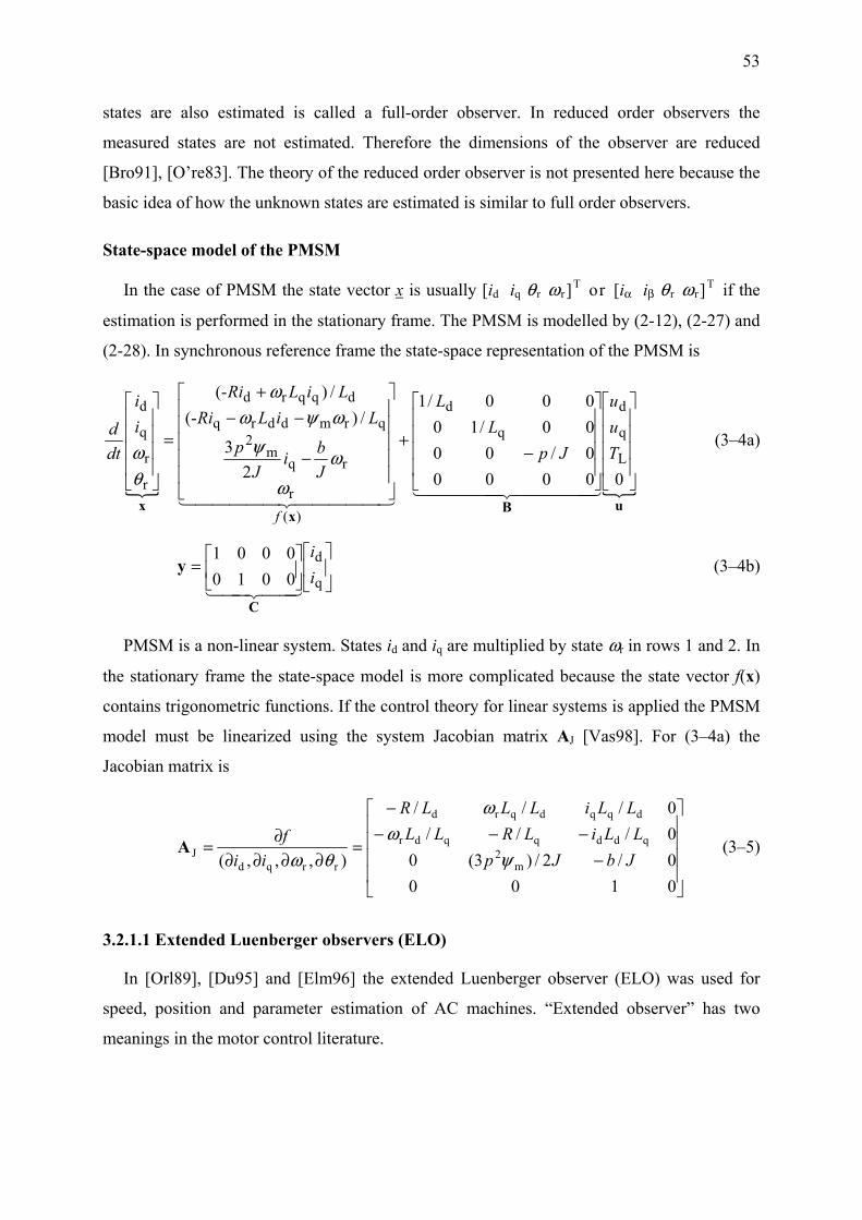
53
states are also estimated is called a full-order observer. In reduced order observers the
measured states are not estimated. Therefore the dimensions of the observer are reduced
[Bro91], [O’re83]. The theory of the reduced order observer is not presented here because the
basic idea of how the unknown states are estimated is similar to full order observers.
State-space model of the PMSM
In the case of PMSM the state vector x is usually [id iq θ r ω r ]T or [iα iβ θ r ω r ]T if the
estimation is performed in the stationary frame. The PMSM is modelled by (2-12), (2-27) and
(2-28). In synchronous reference frame the state-space representation of the PMSM is
uBx
x
⎥⎥⎥⎥
⎦
⎤
⎢⎢⎢⎢
⎣
⎡
⎥⎥⎥⎥
⎦
⎤
⎢⎢⎢⎢
⎣
⎡
−+
⎥⎥⎥⎥⎥
⎦
⎤
⎢⎢⎢⎢⎢
⎣
⎡
−
−−+
=
⎥⎥⎥⎥
⎦
⎤
⎢⎢⎢⎢
⎣
⎡
000000/0000/10000/1
23
/)(-/)(-
L
q
d
q
d
)(r
rqm
2qrmddrq
dqqrd
r
r
q
d
Tuu
JpL
L
Jbi
Jp
LiLRiLiLRi
ii
dtd
f
44444 344444 2144444 344444 21
ωωψωψω
ω
θω
(3–4a)
⎥⎦
⎤⎢⎣
⎡⎥⎦
⎤⎢⎣
⎡=
q
d00100001
ii
44 344 21C
y (3–4b)
PMSM is a non-linear system. States id and iq are multiplied by state ωr in rows 1 and 2. In
the stationary frame the state-space model is more complicated because the state vector f(x)
contains trigonometric functions. If the control theory for linear systems is applied the PMSM
model must be linearized using the system Jacobian matrix AJ [Vas98]. For (3–4a) the
Jacobian matrix is
⎥⎥⎥⎥
⎦
⎤
⎢⎢⎢⎢
⎣
⎡
−−−−
−
=∂∂∂∂
∂=
01000/2/)3(00///0///
),,,( m2
qddqqdr
dqqdqrd
rrqdJ JbJp
LLiLRLLLLiLLLR
iif
ψω
ω
θωA (3–5)
3.2.1.1 Extended Luenberger observers (ELO)
In [Orl89], [Du95] and [Elm96] the extended Luenberger observer (ELO) was used for
speed, position and parameter estimation of AC machines. “Extended observer” has two
meanings in the motor control literature.

Model based estimators 54
1) Linear observer (3–1) is used to estimate the states of a non-linear system. The non-
linear model is linearized every time the estimator algorithm is computed [Bol99],
[Vas98].
2) In addition to 1) the parameters of the model are also estimated [Orl89], [Du95].
If the estimation error x~ is assumed to be small, the non-linear model can be replaced by
AJ (3–5) [Du95], [Elm96]. The discrete time equation of the full order ELO [Du95] is
presented in (3–6). The derivation of (3–6) can be found in [Du95], [Elm96], [Orl89],
[Son00].
( ) ( ))k()k()k()1-k|k(ˆ)k()k()1-k|k(ˆ)k|1k(ˆ s)k(
Js gKyBuxCKAxxL
+++⎟⎟⎟
⎠
⎞
⎜⎜⎜
⎝
⎛−+=+
=
tt44 344 21
(3–6)
The notation x(k|k-1) means that the value of vector x at time instant k is based on the
information from the previous sampling period. The states of the PMSM are estimated by the
ELO using a following four step algorithm:
1. Specify observer poles. Construct a suitable observer matrix L(k) (3–6) with specified
poles. L has the same purpose as F in the linear observer (3–3). This step can be done off-
line.
2. Calculate g(k) = f(x)(k) - AJ(k). g is the error between the nonlinear model and the
linearized model.
3. Solve K from L(k) = AJ(k) – K(k)C.
4. Calculate the state vector at the next sampling period, (3–6).
It is easy to see that the computational requirements of the ELO algorithm are demanding.
AJ is updated at every sampling interval. Therefore the gain matrix K is also constantly
calculated, step 3. Solving K from L(k) is a time consuming operation. In practice the
estimator structure can be greatly simplified without considerable losses in the dynamic
performance. The following section gives a few examples of simplified deterministic
observers.
3.2.1.2 Examples of simplified state observers for speed and position tracking
In [Jon89] the non-linear model of the PMSM in synchronous reference frame (3–4) was
directly used in the observer equation (3–2). Ax was replaced by f(x) in (3–2). It was stated
that the large signal stability of the estimator is difficult to prove. However, it was found in
the simulations that the linearized model predicted the behaviour of the non-linear observer
with a good accuracy. Compared to the ELO the estimator algorithm was greatly simplified.

55
In [Sep92] the observer of [Jon89] was further developed. The gain matrix K was constant in
[Jon89] but in [Sep92] gain scheduling was used. K was not updated in every sampling
period. However, a different gain matrix was used in the low and high speed regions.
In [Low93] the PMSM model in the rotor reference frame (3–4) was linearized using
measured currents id and iq. It is possible now to write a state-space model where A (3–1) is
time-variant but linear.
xCxy
uBx
A
x
]011[
0/00
0/1000/1
/2
30
/)(/-0/0/-
rr
L
q
d
q
d
r
q
d
m2
qddmq
dqqd
r
q
d
===
⎥⎥⎥⎥
⎦
⎤
⎢⎢⎢⎢
⎣
⎡
⎥⎥⎥
⎦
⎤
⎢⎢⎢
⎣
⎡
−+
⎥⎥⎥
⎦
⎤
⎢⎢⎢
⎣
⎡
⎥⎥⎥⎥⎥⎥
⎦
⎤
⎢⎢⎢⎢⎢⎢
⎣
⎡
−
−−=⎥⎥⎥
⎦
⎤
⎢⎢⎢
⎣
⎡
ωθ
ωψψ
ω
dtd
Tuu
JpL
Lii
JbJ
p
LLiLRLLiLR
ii
dtd
4444 34444 21
4444444 34444444 21
(3–7)
The position estimate is obtained by integrating the estimated ω r. (3–7) can be directly used in
the equation of the linear full-order observer (3–2). After the eigenvalues of the error
dynamics (3–3) have been chosen the gain matrix K must be determined. Now A is a function
of currents. Therefore K (3–2) must be updated on-line. A simple method is to use a look-up
table. In practice A is a function of iq only because id is usually small or controlled to zero.
Thus only a one-dimensional table is needed.
3.2.2 Non-linear state observer
The observer based speed and position estimators described above are based on linear
control theory. There are also techniques where the process is linearized using a suitable
feedback structure. No gradient matrix calculations are needed. One of the non-linear
strategies is the “exact linearization” technique [Isi85]. Using this method it is possible to
construct a speed control system for a PMSM where the non-linear effects such as cross
coupling between d and q axis equations are eliminated [Sol00]. This model based non-linear
state-feedback control requires information on all four states of the PMSM (3–4). If
mechanical states are not measured they can be estimated using a full-order [Sol00], [Guc01]
or reduced-order [Sol96] observer also based on the “exact linearization” theory. This non-
linear method can also be used to estimate speed and position for conventional vector control
[Sol95].

Model based estimators 56
The state observer based on “exact linearization” theory is presented in (3–8) [Sol00]. The
observer algorithm is performed in the stationary reference frame. It is an extended version
because the load torque is also estimated.
⎥⎥⎦
⎤
⎢⎢⎣
⎡
−−
⎥⎦
⎤⎢⎣
⎡+
⎥⎥⎥⎥⎥⎥⎥⎥⎥⎥
⎦
⎤
⎢⎢⎢⎢⎢⎢⎢⎢⎢⎢
⎣
⎡
−−+−
+−++
=
⎥⎥⎥⎥⎥⎥
⎦
⎤
⎢⎢⎢⎢⎢⎢
⎣
⎡
+
ββ
αα
r2r1
)(
r
rL
rβrαm
2βrrmβ
αrrmα
L
r
r
β
α
ˆˆ
ˆcosg-ˆsing
0ˆ
ˆˆ
)ˆcosˆˆsinˆ(2
3
//)ˆcosˆˆ(-//)ˆsinˆˆ(-
ˆˆˆ
ˆˆ
iiii
Jb
JT
iiJ
p
LuLiRLuLiR
T
ii
dtd
f
θθω
ωθθψθωψθωψ
θω
ΓK
Bux44444444 344444444 21
(3–8)
where
⎥⎥⎥⎥
⎦
⎤
⎢⎢⎢⎢
⎣
⎡
−= −−
)ˆ/(ˆsin)ˆ/(ˆcos00
ˆcosˆsin0000100001
rmrrmr
1mr
1mr
ωψθωψθψθψθ
LLLL
Γ
K is 4×2 constant matrix. g1 and g2 are also constant gains. A tedious derivation of the non-
linear gain matrix Γ and the proof of stability using Lyapunov’s theory is presented in
[Guc01], [Sol95], [Sol00].
Compared to ELO (3–6) the algorithm is computationally much more effective. There is no
need for complicated matrix operations or gain scheduling. The “exact linearization” method
is mathematically elegant compared to the observers presented above. The stability of the
observer can be proven. Gains K, g1 and g2 are constants and need not to be updated.
3.2.3 Stochastic state observer (Kalman filter)
Kalman filter is a state observer which gives a linear and minimum error variance
algorithm to optimally estimate the unknown states of a dynamic system from noisy data
taken at a discrete time. The structure of the Kalman filter is similar to (3–2). In the Kalman
filter the selection of gain K is based on the stochastic properties of the system [Gre93],
[Vas98]. The model is usually presented in a discrete form.
)k()k()k(
)k())k()k(()k()1k( svCxy
wBuAxx+=
+++=+ xt (3–9)
w and v are zero mean Gaussian noises with covariance matrices Q and R. The system noise
w takes into account the system disturbances (unknown load torque) and parameter errors of
the model. v represents the measurement noise. Noise vectors w and v are independent of the

57
system state vector x if v is not correlated with a process noise w. Q is a 4×4 diagonal matrix
and R is a 2×2 diagonal matrix in the case of the PMSM.
A linear Kalman filter is a two-stage algorithm
( )
))1-k|k(ˆ)k(()1-k|k(ˆk)|k(ˆ))1-k()1-k|1-k(ˆ)1-k|1-k(ˆ)1-k|k(ˆ s
xCyKxxBuxAxx
−+=++= t
(3–10)
where the next value for x is first predicted using the previous value of input vector u and
state vector x. The predicted state vector )1k|k(ˆ −x is then corrected using the error between
the measured output and the predicted output )1k|k(ˆ −xC . For Kalman gain K can be written
1TT )( −+= RCPCPCK (3–11)
P is a state covariance matrix [Gre93], [Vas98]. In the linear case K is a predetermined
constant matrix. In the non-linear case K and P are updated between prediction and correction
steps (3–10) at every sampling interval. The algorithm is called an extended Kalman filter
(EKF). The software implementation is a similar type multistep algorithm as that presented in
Section 3.2.1.1. If an EKF is used to estimate the states of the PMSM the matrix A (3–10) is
replaced by f(x) (3–4). Jacobian matrix AJ (3–5) is needed when the state covariance matrix P
is updated.
Detailed information about EKF can be found in [Bol99], [Bol01], [Bol03], [Dha91],
[Gre93]. Calculations of K and P are time consuming operations. The computational burden
is comparable to an extended Luenberger observer.
Tuning of the Kalman filter is done by adjusting the coefficients of Q and R. Matrices Q
and R affect both the transient performance and steady state operation. The following tuning
principles are given in [Vas98]: If elements of Q are increased a greater uncertainty in the
machine model is assumed. Large Q increases K. The measurements will be more heavily
weighted. If elements of R are increased the measurements are assumed to be noisy and will
be weighted less by the EKF. The elements of K will decrease resulting in a lower transient
performance.
In [Bol03] the selection of Q, R and initial value of P were studied through experimental
tests and simulations. It was found that the per unit values of the current and motor
parameters of surface magnet PMSM vary in a narrow range regardless of motor size.
Therefore it is possible to find covariance matrices suitable for all standard PMSM drives. In
practice some fine tuning should be done but it is claimed in [Bol03] that an effective and
general initial guess has been found for EKF settings in sensorless PMSM drives.

Model based estimators 58
3.2.4 General properties of state observers in sensorless control of PMSM
Several state observers where speed and position were estimated by tracking the measured
stator currents were briefly discussed in Sections 3.2.1 – 3.2.3. ELO, EKF and the observer
based on the “exact linearization” (3–8) were compared by simulations in [Esk02]. There
were no significant differences between the performances of the methods tested. However, the
computations required by those three full order observers are different.
Computations required by the non-linear observer (3–8) are: two divisions, 36
multiplications and 17 additions. The algorithm contains several trigonometric operations.
Sine and cosine of the rotor position may be taken from predetermined tables. Using the look-
up tables is a fast operation compared to time consuming approximation algorithms. In EKF
algorithm there are 125 multiplications and 78 additions. In both methods parameter
dependent constants are calculated off-line and multiplications with zero are eliminated. If the
parameters are estimated on-line they can be updated in the slower time level compared to the
estimator algorithm.
Computational requirements were also compared with Matlab running in the personal
computer with Intel Pentium processor. Both algorithms were driven 105 times in a for-loop.
Time was measured using Matlab’s timer functions.
If the relative duration of the “exact linearization” for-loop is 1, the time needed by EKF is
approximately 3.6. This ratio is in agreement with the number of computations of these
methods. ELO was also tested using the same method and was ten times slower than EKF.
However, this result is not valid in practice because the gain matrix K (3–6) was solved by
Matlab’s PLACE function which is not designed for real-time applications.
The non-linear observer would be fairly easy to implement using common
microcontrollers. EKF and ELO require more optimization of algorithms if they are applied in
practice.
Although the algorithms discussed above have their own features there are also properties
and problems common to all state observers.
1. Instability at zero speed. Theoretically this means that the PMSM model is not
observable if ω r is zero [Åst97]. This is a common property for all model based estimators. If
currents and voltages are DC-signals there is not enough information on rotor position.
2. The Need for the mechanical model. The states are corrected using the error between
measured states and their estimates. All four states [id iq θ r ω r] of the PMSM are needed to
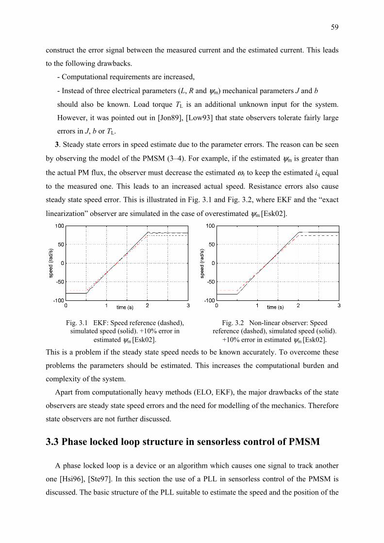
59
construct the error signal between the measured current and the estimated current. This leads
to the following drawbacks.
- Computational requirements are increased,
- Instead of three electrical parameters (L, R and ψm) mechanical parameters J and b
should also be known. Load torque TL is an additional unknown input for the system.
However, it was pointed out in [Jon89], [Low93] that state observers tolerate fairly large
errors in J, b or TL.
3. Steady state errors in speed estimate due to the parameter errors. The reason can be seen
by observing the model of the PMSM (3–4). For example, if the estimated ψm is greater than
the actual PM flux, the observer must decrease the estimated ω r to keep the estimated iq equal
to the measured one. This leads to an increased actual speed. Resistance errors also cause
steady state speed error. This is illustrated in Fig. 3.1 and Fig. 3.2, where EKF and the “exact
linearization” observer are simulated in the case of overestimated ψm [Esk02].
Fig. 3.1 EKF: Speed reference (dashed), simulated speed (solid). +10% error in
estimated ψm [Esk02].
Fig. 3.2 Non-linear observer: Speed reference (dashed), simulated speed (solid).
+10% error in estimated ψm [Esk02].
This is a problem if the steady state speed needs to be known accurately. To overcome these
problems the parameters should be estimated. This increases the computational burden and
complexity of the system.
Apart from computationally heavy methods (ELO, EKF), the major drawbacks of the state
observers are steady state speed errors and the need for modelling of the mechanics. Therefore
state observers are not further discussed.
3.3 Phase locked loop structure in sensorless control of PMSM
A phase locked loop is a device or an algorithm which causes one signal to track another
one [Hsi96], [Ste97]. In this section the use of a PLL in sensorless control of the PMSM is
discussed. The basic structure of the PLL suitable to estimate the speed and the position of the

Model based estimators 60
PMSM is illustrated in Fig. 3.3. The phase detector block calculates the error signal ε, which
is a function of the estimation error. The phase detector embodies the control system, the
model of the motor and the measured quantities used to calculate the error signal ε. As will be
seen in the following sections, the position estimation error rrr ˆ~ θθθ −= causes an error
signal which can be written in the form:
)~sin( rθε K= (3–12)
where K is an application specific gain parameter. The error ε can be used to force the
position estimate to its true value using the following non-linear algorithm [Har00]
εω1
r kˆ
=dt
d (3–13)
εωθ2r
r kˆˆ
+=dt
d (3–14)
where k1 and k2 are gain parameters. The structure of the algorithm (3–13), (3–14) can be
considered as a PI controller and an integrator connected in series, Fig. 3.3. The basic
structure shown in Fig. 3.3 can be used in the case of model based and injection estimators.
Every estimation method has its own phase detector system.
I
ε ω
θ
phasedetector
θIk1
k2 +a)
I
ε
ω
θ
phasedetector
θIk1
k2 +
PI-controller
b)
Fig. 3.3 Speed and position estimator using PLL structure. a) Speed estimate is an integral of the
position error, b) speed estimate is the output of the PI controller.
Dynamics of the PLL
The estimate of angular speed of the PMSM can be taken from the output of the integral
branch [Har00], Fig. 3.3a, or from the output of the PI-controller, Fig. 3.3b. The latter is faster
and commonly used in the literature, [And99], [Lee04a], [Mat90]. In this study the slower
version is preferred because it is less sensitive to noise.
To make the analysis of the PLL easier the error ε is linearized by assuming
rrrrr~ˆ)ˆsin( θθθθθ =−≈− . This is a valid assumption if the estimation error is small. It is
also assumed that ε is calculated correctly and without delay. (3–13) and (3–14) are now
written as
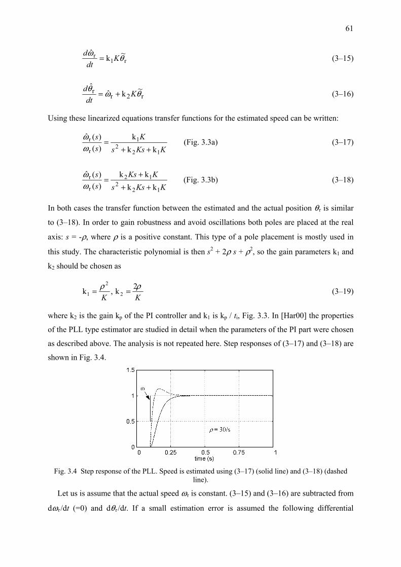
61
r1r ~k
ˆθω K
dtd
= (3–15)
r2rr ~kˆ
ˆθωθ K
dtd
+= (3–16)
Using these linearized equations transfer functions for the estimated speed can be written:
KKss
Kss
122
1
r
r
kkk
)()(ˆ
++=
ωω
(Fig. 3.3a) (3–17)
KKss
KKsss
122
12
r
r
kkkk
)()(ˆ
+++
=ωω
(Fig. 3.3b) (3–18)
In both cases the transfer function between the estimated and the actual position θ r is similar
to (3–18). In order to gain robustness and avoid oscillations both poles are placed at the real
axis: s = -ρ, where ρ is a positive constant. This type of a pole placement is mostly used in
this study. The characteristic polynomial is then s2 + 2ρ s + ρ2, so the gain parameters k1 and
k2 should be chosen as
KKρρ 2k,k 2
2
1 == (3–19)
where k2 is the gain kp of the PI controller and k1 is kp / ti, Fig. 3.3. In [Har00] the properties
of the PLL type estimator are studied in detail when the parameters of the PI part were chosen
as described above. The analysis is not repeated here. Step responses of (3–17) and (3–18) are
shown in Fig. 3.4.
Fig. 3.4 Step response of the PLL. Speed is estimated using (3–17) (solid line) and (3–18) (dashed
line).
Let us is assume that the actual speed ω r is constant. (3–15) and (3–16) are subtracted from
dω r /dt (=0) and dθ r /dt. If a small estimation error is assumed the following differential

Model based estimators 62
equations for estimation error can be written where the noise component n is added to the
linearized error component r~θK .
)~(~
r
2r nK
Kdtd
+−= θρω (3–20)
)~(2~~
rrr nK
Kdtd
+−= θρωθ (3–21)
When the angle error is solved from (3–21) and substituted into (3–20) we obtain the relation
between disturbance n and estimation errors for speed and position.
ns
sK ⎟⎟
⎠
⎞⎜⎜⎝
⎛
+−= 2
2
r )(~
ρρω (3–22)
nssss
K ⎟⎟⎠
⎞⎜⎜⎝
⎛
++++−= 2
22
r ))(2(252~ρρρρρθ (3–23)
The relation between the speed error and noise is a band pass filter with centre frequency ρ
(3–22). The steady state speed error is zero if disturbance n is a DC-signal. This means that
slowly varying disturbances like parameter uncertainties do not produce a speed error in
steady state. This is a clear advantage compared to the observers discussed in previous
sections. Transfer function between position error and noise is a low pass filter with non-zero
DC-gain (3–23). Thus the parameter errors can create a position error in steady state
operation.
3.4 Back-emf estimators
This section deals with estimators where the primary estimated quantity is the back-emf of
the PMSM. First the idea of speed and position estimation directly from voltage equations of
the PMSM (2-12) is discussed in Chapter 3.4.1. Some examples taken from the literature are
presented. Direct estimation from voltage equations is a simple task but leads to problems
with steady state errors if parameters are not accurately known. Therefore the rest of Chapter
3.4 concentrates on methods where a PLL type algorithm is used to remove the steady state
errors. The error signal of the PLL (3–12) in the case of PMSM drive is derived in Section
3.4.2. Section 3.4.3 deals with estimators where the speed is estimated directly from voltage
equations and the effect of parameter errors is corrected by a PLL algorithm. Section 3.4.4

63
deals with the current tracking estimator. This method is also based on the estimated back-
emf information but the error between measured and estimated current is used instead of the
voltage error. The best properties of estimators discussed in Sections 3.4.3 and 3.4.4 are
combined in one algorithm in Section 3.4.5. In this Section 3.4, Ld and Lq do not vary as a
function of the rotor position. The effect of non-sinusoidal flux linkage and inductance
variations are studied by simulations in Section 3.6.
3.4.1 Direct speed and position estimation
A very straightforward strategy to estimate the angular speed ωr of the PMSM is presented
below. The speed is solved directly from the imaginary component of the voltage equation in
the rotor frame (2-12).
m
qeqqeqe
rmddrq
qqq ˆ
ˆˆˆ)(
Ψdt
diLiRu
iLdt
diLRiu
−−=⇒+++= ωψω (3–24)
The subscripts de and qe denote quantity in the estimated rotor reference frame (control
system reference frame). The position estimate is obtained by integrating the estimated speed.
If parameters, currents and voltages are accurately known the PLL algorithm would be
unnecessary because (3–24) gives a correct estimate for the speed. In transients the estimate
would be slightly delayed due to the current control. In practice ωr estimated by (3–24)
always contains a steady state error. Using the actual motor quantities (3–24) can be written in
steady state (current derivatives are zero):
mrdrqrdrqmqeqe2 ˆ/)~sinˆ~cosˆ~sin~cos(ˆ/)ˆ(ˆ ψθθθθψω iRiRuuiRu −−+=−= (3–25)
The subscript 2 in ω denotes the output of the direct speed estimator. The current seen by the
control system is
rdrqqerqrdder~jrre ~sin~cos,~sin~cos θθθθθ iiiiiieii +=−=⇔= (3–26)
The current control drives the average of ide to zero (in this thesis id,ref = 0). The steady state
d axis current is
rqd~tanθii = (3–27)
The rotor frame voltage equation (2-12) and (3–27) are substituted into (3–25). Now the
speed estimate in steady state is:

Model based estimators 64
)~sin~cos(ˆ
~~sinˆ
)(~cosˆ
ˆ rdrqm
rqm
qdr
m
mr2 θθ
ψθ
ψθ
ψψωω iiRi
LL++⎟⎟
⎠
⎞⎜⎜⎝
⎛ −+= (3–28)
The system is unstable without PLL correction if parameter errors force 2ω to be smaller
than |ω r|. Let us consider the case when ω r > 0, iq > 0, 0ˆ mm <−ψψ and .0~ =R The position
error is initially zero. The estimate given by (3–28) is smaller than ω r and the speed control
tries to drive the speed error to zero by increasing the q axis current reference. The position
estimate is the integral of the speed estimate. Now the position error r~θ increases because (3–
28) gives too small estimate for speed. Increased position error further decreases the estimated
speed. This creates a positive feedback. If 0~ <R the effect is similar. In the opposite case the
system is stable but a steady state position error remains. If parameter errors increase the
absolute value of the speed estimate 2ω the system stabilizes to the operating point where the
left and right hand sides of (3–28) are equal. The speed error is zero in steady state. Analytical
solution of the steady state position error would lead to a very complicated expression. It can
be checked by simulations that rather small parameter errors create significant steady state
position errors.
This parameter sensitivity is the main reason why the real part of the voltage model (2-12)
should be also exploited. As will be explained in the next section (3.4.2) the d axis voltage
equation contains position error information.
Estimators in the literature
In [Pii04] the speed is estimated directly using the q axis voltage model (3–24). The
parameter sensitivity of the estimator was decreased by an additional PM flux estimator. The
total estimator algorithm is simple and the performance in experimental tests was fairly
satisfactory [Pii04]. However, the position error can be significant if the R and ψm are not
accurately known.
The paper published by Kim and Sul [Kim97] is a widely cited publication where the
speed and position are determined directly from the estimated back-emf in the estimated
synchronous reference frame. A non-salient PMSM was assumed. If Ld = Lq = L the voltage
model in the estimated rotor frame can be approximated as
65
43421
43421
qe
mrderqe
qeqe
de
mrqerde
dede
~cosˆ
~sinˆ
e
e
Lidt
diLRiu
Lidt
diLRiu
θψωω
θψωω
+++≈
−−+≈
(3–29)
Flux components Lid, Liq are multiplied by the estimated speed because it is the derivative
of the position angle of the estimated reference frame. Equation (3–29) will be further
discussed in Section 3.4.2. In [Kim97] current derivatives were removed using the idea of
“electrical steady state”. Current sampling and control of currents were performed more
frequently than the speed control and the estimator. The longer time interval is called an
“estimation period”. Current samples from the end of the estimation period are used. It was
assumed that even in speed transients the currents are constants at the end of the estimation
period. Thus dire/dt = 0. The estimated position used in current control was fixed to a constant
for one estimation period. If the estimated angle is constant rr ˆ/ˆ ωθ =dtd = 0. Now the
derivatives are removed from (3–29) and it can be written for the position error
rrrrm
rrmqe*qede*de
qede ~~tan~cos
~sin θθθωψθωψ
≈==−+−
=RiuRiu
ee (3–30)
In (3–30) voltages ude* and uqe* are not the same as steady state voltages of (3–29) because
the estimated speed is zero. Position error (3–30) is added to the previous estimate at each
estimation interval. Thus it can be considered an input of the discrete time integrator. The
position is calculated:
sremfremfemf ˆ)1-k(ˆ~)1-k(ˆ)k(ˆ tωθθθθ +=+= (3–31)
where ts is the sample time. It should be noted that π/2 rad must be subtracted from the angle
θemf to obtain the estimate of the rotor position.
This position estimator is a tracking type method where the actual error signal is
-ude* + Ride. If the position estimate is smaller than the actual position the error ( rrr ˆ~ θθθ −= >
0). The position estimate (3–31) will also be too large. As a result ede increases and the
estimated position will be corrected toward the actual value during the next sampling period.
The same idea natually works when the position estimate is leading the actual position.
If ide is small the parameter R in the denominator of (3–30) only changes the gain of the
position error signal (3–31) if it is not accurately known. Therefore parameter errors have no
significant influence on the steady state position estimate.

Model based estimators 66
In [Kim97] the speed is estimated using a separate algorithm where the length of the
estimated back-emf is divided by PM flux. The speed estimate is naturally sensitive to errors
of ψm and R. The estimate of ψm is corrected by a fairly simple algorithm. The estimated
speed is compared to the speed estimated directly from the position error, srr /~ˆ tθω = (3–31).
This signal is noisy but in steady state its average is equal to the actual speed. The difference
between the speed estimates is the input for a PI controller and the output of the controller is
used to correct the estimated ψm.
The algorithm introduced in [Kim97] has a simple structure and good position tracking
properties. The main drawbacks are the parameter sensitive speed estimator and the need for
parameter correction.
In [Bat00] the rotor position of the PMSM is estimated by a state observer based on the
voltage equation in stationary frame. This method suffers from the same drawbacks as the
state observers discussed in previous sections. In the position estimator the gain matrix should
be updated when ω r changes. The estimated speed contains steady state errors if R or ψm are
not correctly estimated. The position estimate has been reported to be rather insensitive to
parameter errors [Bat00].
3.4.2 Voltage equations in the estimated synchronous reference frame
The voltage equation of the PMSM is analysed in steady state conditions. The control and
estimator algorithms are performed in the estimated synchronous reference frame. The
frequency converter is assumed to be ideal. There is no voltage error between the voltage
reference and the actual stator voltage. Higher order harmonics of flux linkage and
inductances are ignored. In that case voltages ude and uqe are the voltage reference signals
ude,ref and uqe,ref. These signals are the outputs of the d and q axis current controllers. The
voltage equations of the PMSM in the actual rotor frame are
)( mddr
qqqq
qqrd
ddd
ψω
ω
+++=
−+=
iLdt
diLRiu
iLdt
diLRiu
(3–32)
Current derivatives can be ignored because steady state operation is analysed. The voltage
equation (3–32) is transformed into the estimated rotor reference frame, r~jrre θeuu = , Fig.
3.5a. The voltage components in the estimated d,q frame are

67
( )( ) rmrqdrrqer
2dr
2qderqeqe
rmrr2
dr2
qqeqdrrderdede~cos)(~sin~cos)~cos~sin(ˆ
~sin)~sin~cos()(~sin~cosˆ
θψωθθθθω
θψωθθθθω
+−−+−−=
−++−−=
LLiLLiRiu
LLiLLiRiu (3–33)
where rrr ˆ~ θθθ −= . The voltages ude, uqe in (3–33) are the steady state outputs of the current
controllers (voltage references). Motor parameters (R, Ld, Lq, ψm) are accurately known.
d
qe
de
q
θ~θ
θr
r α
a)
β
ude
uuqe uq
ud
d
qe
de
q
θ~θ
θr
r α
c)
β
edeeqe
e
d
de
q
θ~θ
θr
r α
a)
β
u
ud
d
de
q
θ~θ
θr
r α
a)
β
u
ud
d
qe
de
q
θ~θ
θr
r α
b)
βiqe iq
id
d
qe
de
q
θ~θ
θr
r α
β
d
qe
de
q
θ~θ
θr
r α
β
i
Fig. 3.5 Transformation between actual and estimated rotor reference frame: a) u b) i c) back-emf.
The position error r~θ is unknown to the estimator algorithm. The software can calculate
the steady state voltage by the following expression
mrdedrqeqe
qeqrdede
ˆˆˆˆˆˆ
ˆˆˆˆ
ψωω
ω
++=
−=
iLiRu
iLiRu (3–34)
The parameters used in (3–34) are estimates. Let us assume there are no parameter errors. The
angular speed is estimated. In steady state the estimated speed is equal to the actual speed if
the PLL algorithm is used. If (3–34) is subtracted from (3–33) it is possible to write the
following voltage errors for the d and q axes.
( )( ) )1~(cos)~cos~sin)((~sinˆ~ˆ
~~sin)~sin~cos)((~sinˆ~ˆ
rmrrqerdeqdrrqeqeqe
rmrrmrrqerdeqdrrdedede
−+−−−==−
−≈−+−−==−
θψωθθθω
θψωθψωθθθω
iiLLuuu
iiLLuuu(3–35)
de~u is the d axis component of the back-emf vector e, Fig. 3.5c. de
~u is a suitable error signal
for PLL algorithm (3–12). Saliency has only a negligible effect because ide and r~sinθ are
controlled to zero in steady state. If the d axis error is compared to (3–12) the gain parameter
K is now -ω rψm.
In practice the input for PLL ( de~u ) can be solved using the d axis voltage reference signal
and (3–34). In steady state ude = ude,ref (3–33). It can be seen from (3–35) that the voltage
reference ude,ref > ûde if r~θ < 0. If r
~θ > 0, ude,ref < ûde. The d axis voltage can be estimated:

Model based estimators 68
qeqrˆˆ iLω− = ûde (3–34) if ide is controlled to zero in steady state. The d axis component of the
back-emf can be approximated as
)ˆsign()ˆˆ(~rqeqrrefde,de ωω iLuu −−≈ (3–36)
The result must be multiplied by the sign of the rotor speed because the sign of the d axis
component of the back-emf is dependent on the sign of ω r (3–35).
The q axis voltage error (3–35) is not a suitable input for the PLL algorithm. However,
uq,ref is proportional to ω r . Thus it contains information which can be exploited in the speed
estimation process.
3.4.3 Back-emf estimator with the phase locked loop structure
Matsui introduced in [Mat90] a simple estimator based on the voltage equation of the
PMSM transformed to the estimated rotor frame (3–33). The rotor speed is estimated using
two separate algorithms. The speed is estimated primarily by the direct method using the q
axis voltage equation (3–24). As discussed in 3.4.1, direct speed estimators are sensitive for
parameter errors. Matsui’s novel idea was to correct the output of the direct estimator with a
PLL type algorithm. The d axis voltage equation (3–33) in the estimated rotor reference
frame, Fig. 3.5, contains information on the position error. The input signal for the PLL is
calculated by (3–36). The output of the PLL is added to the direct estimate, 2ω (3–24). Finally
the position is estimated by integrating the sum of two speed estimates. The block diagram of
the estimator is presented in Fig. 3.6.
I
ude ωr,filt
θr
Ik1
k2 +
-ude,ref+Ride-ωrLqiqeωr
PMSM control system
ureire
iabc
+
(uqe,ref-Riqe-Lq(diqe/dt)-ωrLdide)/ψm ω2
LP
ω1ωr2
+ωr
ire
ure
ωr,filt Fig. 3.6 Speed and position estimator with feedforward branch and PLL in synchronous frame.
Matsui’s voltage model method.
Matsui’s original estimator is not equal to the Fig. 3.6. In [Mat90] the speed estimate used
in the speed control was the sum of 1ω and 2ω ( 2rω in Fig. 3.6). In this thesis the output of
the integrator of the PLL was used as an speed estimate for speed control purposes due to the
lower noise sensitivity.

69
In Fig. 3.6 the derivative of ide is not included in the PLL input because ide is held at zero
and its amplitude is rather small in transients too. Therefore ide can be completely omitted
from the software implementation without significant impairment of the dynamic
performance.
The model based algorithm introduced by Matsui has inspired several authors to publish
methods closely related to [Mat90]. The PLL type voltage model estimator is studied also in
[Har00], [Sak01], [Lee04a]. In [Har00], [Lee04a] the PLL algorithm was used without the
direct speed estimator (3–24). In [Sak01] the position error signal was calculated by arctan
method as in [Kim97], (3–30). The signal was input for the PLL algorithm. No direct speed
estimator was used. These methods utilise only the d axis back-emf information.
[Mat90] is studied in detail in this thesis because it utilises the information of both the real
and imaginary axes of the estimated back-emf. Compared to state observers it has a rather
simple structure. The steady state speed error is zero even if the motor parameters are not
accurately known. In the following sections [Mat90] is called Matsui’s voltage model method.
Matsui’s estimator in stationary reference frames
The author presented a “novel” voltage model based estimator in [Esk03]. In fact, this
estimator method is a direct counterpart to [Mat90] in the stationary reference frame. The
block diagram is illustrated in Fig. 3.7. In [Esk03] the estimator was proposed for PMSMs
with a saliency ratio close to unity (Ld = Lq = L). The fundamental frequency voltage equation
of the PMSM (3–32) can be written in stationary reference frame as
.
ˆ1)
ddˆˆ(
d
ˆdˆ
jd
dd
d
m
π/2)rˆj(s
ssref
rr
rjmr
ss
sss
ψθω
ψωψ
θ
θ
⋅⋅−−==⇒
⋅++=+=
+43421
444 3444 21 wy
etiLiRu
t
etiLiR
tiRu
(3–37)
y is a back-emf phasor whose length is proportional to the angular speed and its angle leads
the d axis π/2 rad. w is a phasor with a length of 1 and it leads the estimated rotor position by
π/2 rad. If the imaginary part of the product yw* (cross product of vectors) is zero, the phasors
w and y are in phase and the estimated position angle is correct, provided that the parameters
are known. The angle increment is mainly composed of Reyw*. Imyw* is an error signal
which is an input for the PLL algorithm.

Model based estimators 70
R
+−
L
+−
ωr
is
us
disdt
wαyα+wβyβ
PI
+
+ψ
m-1
dθrdt I
θr
LP
e j(x+π/2)
y
w
unit vector
ed
Re(ye*):
Im(ye*): wαyβ-wβyα
phase detector
Fig. 3.7 Back-emf estimator with feedforward branch in the stationary reference frame.
Other papers applying stationary frame equations have also been published. In [Yin02] the
position was estimated in stationary frame using three-phase equations. [Yin02] was
improved using PLL structure in [Yin03] which is a three phase counterpart of [Esk03].
3.4.3.1 Estimation of the speed and position using only the phase locked loop
The direct branch of the speed estimation process was discussed in Section 3.4.1. In this
section the PLL branch of the Matsui’s voltage model method is studied. Equations for the
gains of the PI controller are presented and parameter sensitivity is analysed.
I
ωr
θr
Ik1
k2 +
-ud,ref+Ride-ωrLqiqeωr
PMSM control system
ude,refire
iabc
ωr
ude(3-36)
Fig. 3.8 Block diagram of the back-emf estimator in the rotor reference frame.
The gain parameter K of the PLL (3–12) is speed dependent (-ω rψm) as discussed. This is
a drawback because the gains k1 and k2 of the PI controller, Fig. 3.6, Fig. 3.8 must be a
function of the estimated speed if the bandwidth of the PLL is kept constant. In the original
paper [Mat90] constant gains were used. Because K is proportional to speed the gains k1 and
k2 must be inversely proportional to the estimated speed. This leads to infinite gains at zero
speed. Gains k1 and k2 are limited when the estimated speed approaches zero [Har00]. Thus
the bandwidth of the speed control loop is reduced at low speeds. The following gains are
used in this thesis
If lowrˆ ωω > : mr
2
1 ˆˆk
ψωρ= ,
mr2 ˆˆ
2kψωρ= (3–38a)
If lowrˆ ωω ≤ : mlow
2r
1 ˆ)ˆsign(
kψω
ρω= ,
mlow
r2 ˆ
)2ˆsign(k
ψωρω
= (3–38b)

71
The pure PLL estimator has some drawbacks. The rate of convergence at low speeds is
decreased because the gains k1 and k2 must be limited. If the inertia of the drive is small and
fast accelerations are required, the PLL is easily pulled out of phase lock. To prevent this the
poles of the PLL algorithm must be placed far from the imaginary axis. This increases k1 and
k2, which means the noise is more heavily amplified.
In [Wal05] the transient performance of the PLL was improved by boosting the input of
the integrator, Fig. 3.9. The output of the PLL was subtracted from the speed estimate
achieved directly from the length of the estimated back-emf. The result was amplified and
added to the input of the integrator. However, Matsui’s voltage method, Fig. 3.6, Fig. 3.7, is
faster because the direct estimate is not fed through the integrator.
I
εd ωr
θr
Ik1
k2 +
-ud,ref+Ride-ωrLqiqeωr
PMSM control system
ud,refirefia,b,c
+
k3
ieuref
ωr
+−|e|
ψm
Fig. 3.9 Improved PLL estimator [Wal05].
The effect of parameter errors
In steady state the derivative of the speed of the PMSM is zero. The steady state speed
error r~ω is also zero when PLL type algorithm is used. Derivatives of the estimates of speed
(3–13) and position (3–14) are subtracted from the derivatives of the actual quantities. After
subtraction the speed and position error derivatives can be written [Har00]:
⎪⎩
⎪⎨
⎧
=−=
=⇒=−=
0k~
00k~
2rr
~1
r
εω
εεω
θdt
ddt
d
(3–39)
Thus the d axis voltage error signal (3–35) is zero in steady state conditions.
In Section 3.4.2 the equation of the d axis voltage error (position error signal) was obtained
by subtracting the estimator’s ude (3–34) from the actual ude (3–33). Now the same subtraction
is made with parameter errors, R ≠ R and qqˆ LL ≠ . The steady state voltage error signal of d
axis can be written:
( ) ωωθψθθωω ˆrmrqerdedqrdeqeqrde |0~sin)~sin~cos)((~~~==−+−−−= iiLLiRiLu (3–40)

Model based estimators 72
where q~L = qq LL − and R~ = RR ˆ− . ide is assumed to be zero. The position error solved
from (3–40) is
⎪⎪⎩
⎪⎪⎨
⎧
=
≠⎟⎟⎟
⎠
⎞
⎜⎜⎜
⎝
⎛
−−
−++−
=
−
−−
dq1
mqeq1-
dqmqedq
2mq
2qedq1
)~(sin-
)(2
~)(411sin~
LLiL
LLiLL
LiLL
ψ
ψψ
θ (3–41)
If ide is controlled to zero, the effect of the resistance error vanishes. PM flux ψm is not
used in the estimation process. Thus the Lq is the only error source in steady state if the speed
and the position are estimated using only the PLL, Fig. 3.8. The position error is proportional
to iqe (3–41). It should be noted that iqe is also a function of position error. However, in the
case of tolerable errors iqe ≈ iq.
3.4.3.2 Discrete time implementation
The equations of the back-emf estimator must be converted into discrete time form before
they can be implemented with a microcontroller. In this study the backward Euler
approximation [Åst97] is used. Discrete time transfer function is obtained by replacing the
Laplace variable s by (z-1)/zts. The discrete time algorithm of the PI controller of the PLL,
Fig. 3.6, Fig. 3.8, can be written
2des1de1depdei
sp11 )k(~)k(~)1k()k(~)k(~)1k()k( kutkuuku
ttk
++−=++−= ωωω (3–42)
where ts, ti and kp are sample time, integration time and gain respectively.
The calculation of 2ω contains the derivative of iq. The discrete derivative is
(iqe(k) - iqe(k-1))/ts. After LP filtering of the derivative 2ω is calculated by the q axis voltage
equation (3–24). The position estimate is updated by the following integral algorithm.
( ))()()1(ˆ)(ˆ 21srr kktkk ωωθθ ++−= (3–43)
In practice the estimated speed must be filtered before it can be used in the speed control
loop. The first order LP filter can be written in discrete form as follows.
)k(ˆ)1k(ˆ)k(ˆ rs
sfiltr,
sfiltr, ω
τω
ττω
tt
t ++−
+= (3–44)
21r ˆˆˆ ωωω += and τ is an inverse of -3 dB corner frequency, τ = 1/(2πf-3dB)

73
3.4.4 Back-emf estimator based on the current tracking
Matsui also introduced another interesting model based estimator [Mat92], Fig. 3.10. The
estimator was compared to [Mat90] in [Mat96] where it was called a current model estimator.
“Current model” is a somewhat misleading name because the estimation is based on the same
equations (3–32) as Matsui’s “voltage model” method. The idea of [Mat92] is to estimate ω r
and θ r by tracking the measured currents in the estimated synchronous reference frame.
If the basic rotor frame voltage equation (3–32) is transformed to the estimated rotor
reference frame (3–33), the derivatives of ide and iqe can be written
⎟⎟⎟
⎠
⎞
⎜⎜⎜
⎝
⎛
−−−=
⎟⎟⎟
⎠
⎞
⎜⎜⎜
⎝
⎛++−=
4434421
4434421
qe
rmrdedrqeqeq
qe
de
rmrqeqrdeded
de
~cosˆ1
~sinˆ1
e
e
iLRiuLdt
di
iLRiuLdt
di
θψωω
θψωω
(3–45)
Some information is omitted when current derivatives (3–45) are solved from (3–33). A
rather small position error is assumed. In that case sin( r~θ ) and the effect of saliency (Ld - Lq)
are vanishing and can be excluded from (3–33) before (3–45) is written. ede and eqe are d and
q axis components of the back-emf in the estimated synchronous reference frame.
If the derivative of current is known it is possible to write the following discrete time
expression for the current at the next sampling period.
)/()k()1k()/()k()1k(
qesqeqe
desdededtditiidtditii
+=++=+
(3–46)
Voltage components ede and eqe are unknown in (3–45). Therefore the estimator must
calculate the derivatives using the basic rotor frame voltage equation (3–32).
( )
( )mrdedrqeqeq
qe
qeqrdeded
de
ˆˆˆˆˆˆ1ˆ
ˆˆˆˆ1ˆ
ψωω
ω
−−−=
+−=
iLiRuLdt
id
iLiRuLdt
id
(3–47)
In the case of Equation (3–47) the current components predicted by the estimator software are
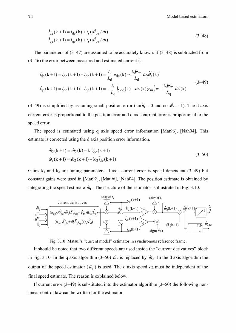
Model based estimators 74
)/ˆ()k()1k(ˆ)/ˆ()k()1k(ˆ
qesqeqe
desdede
dtidtii
dtidtii
+=+
+=+ (3–48)
The parameters of (3–47) are assumed to be accurately known. If (3–48) is subtracted from
(3–46) the error between measured and estimated current is
( ) )k(~)k(ˆ)k()1k(ˆ)1k()1k(~
)k(~)k()1k(ˆ)1k()1k(~
rq
msmrqe
q
sqeqeqe
rrd
msde
d
sdedede
ωψψω
θωψ
Lt
eLt
iii
Lt
eLt
iii
−≈−−=+−+=+
≈=+−+=+ (3–49)
(3–49) is simplified by assuming small position error (sin r~θ = 0 and cos r
~θ = 1). The d axis
current error is proportional to the position error and q axis current error is proportional to the
speed error.
The speed is estimated using q axis speed error information [Mat96], [Nah04]. This
estimate is corrected using the d axis position error information.
)1k(~k)1k(ˆ)1k(ˆ
)1k(~k)k(ˆ)1k(ˆ
de22r
qe122
+++=+
+−=+
i
i
ωω
ωω (3–50)
Gains k1 and k2 are tuning parameters. d axis current error is speed dependent (3–49) but
constant gains were used in [Mat92], [Mat96], [Nah04]. The position estimate is obtained by
integrating the speed estimate rω . The structure of the estimator is illustrated in Fig. 3.10.
ωr,filt
θrk1
k2 (ude-Ride+ωrLqiqe)(ts/Ld)
ω2 ωr(k+1)
LP
(uqe-Riqe-ω2(Ldide+ψm))(ts/Lq)+
ide(k+1)
++-
+ -
iqe(k+1)
iqe(k+1)
ide(k+1)
+ω2(k+1)
+ I
ω1(k+1)
delay of ts
ire
ure
sign(ω2)
delay of ts
ωr
current derivatives
Fig. 3.10 Matsui’s ”current model” estimator in synchronous reference frame.
It should be noted that two different speeds are used inside the “current derivatives” block
in Fig. 3.10. In the q axis algorithm (3–50) rω is replaced by 2ω . In the d axis algorithm the
output of the speed estimator ( rω ) is used. The q axis speed ω2 must be independent of the
final speed estimate. The reason is explained below.
If current error (3–49) is substituted into the estimator algorithm (3–50) the following non-
linear control law can be written for the estimator

75
)/(~cos)k()/1)(k(ˆ)1k(ˆ qs1mrrqms122
qe
LtkLtke
44 344 21ψθωψωω −+=+ (3–51)
)/(~sin)k()1k(ˆ)1k(ˆ ds2
de
rmr2r Ltke
44 344 21θψωωω ++=+ (3–52)
(3–51) is a discrete time first order low pass filter with time constant τ = -(ts + Lq/(k1ψm)).
Thus 2ω converges to ω rcos r~θ . The bandwidth of the LP filter is a function of gain k1. LP
filtered speed 2ω is corrected by the sine of the position error multiplied by the gain k2, Fig.
3.11. k2 must be multiplied by -1 if ω r is negative, Fig. 3.10, because the sign of the d axis
error signal is a function of the sign of ωr (3–49).
ω2
θr
ω1
LP
+ωr
ωrψmcos( )
k2ωrψmsin( )
Fig. 3.11 Control law for the Matsui’s current model method.
The position error is the input for the speed estimation process, Fig. 3.11, and it is the
integral of the speed error rr ωω − . In steady state the output rω is constant. Thus the speed
error must be zero in steady state operation. This also holds in the case of erroneous
parameters.
The basic structure of the “current model” method is similar compared to the “voltage
model” method, Fig. 3.6. The q axis voltage equation is used to give a fast direct estimate for
the speed which is corrected by monitoring the d axis component of the back-emf. However,
this method contains no PLL structure. Therefore parameter errors create large position errors.
Effect of parameter errors
The parameters R and ψm are not accurately known when the equation of current error is
calculated (3–49). The q axis error can be written
( )qemrrmrq
sqe
~ˆ)k(ˆ~cos)k()1k(~ iRLt
i +−−=+ ψωθψω (3–53)
When (3–53) is substituted into (3–50) the equation for 2ω is
( )mqerqms1qms122 /~~cos)k()/()/ˆ1)(k(ˆ)1k(ˆ ψθωψψωω iRLtkLtk +−+=+ (3–54)
Equation (3–54) is a discrete LP filter with DC gain mm ˆ/ψψ . Now the speed estimate 2ω
converges to

Model based estimators 76
( ) mqermr2 ˆ/~~cosˆ ψθψωω iR+= (3–55)
Speed control is unstable if R~ or m~ψ force the speed estimate (3–55) to be smaller than ω r .
Similar behaviour of the direct speed estimator using the q axis voltage model was discussed
in Section 3.4.1. Thus the d axis algorithm must be used to correct the estimated speed (3–55).
In steady state
( ) mqermrdmsr2r21r ˆ/~~cos/)(~sinˆˆ ψθψωψωθωωω iRLtk ++=+= (3–56)
where k2ω r ≥ 0. If small r~θ is assumed: 1~cos r ≈θ and rr
~~sin θθ ≈ . Steady state position error
can solved from (3–56).
dms2r
qemmmrr /)(
)ˆ/~()ˆ/1(~Ltk
iRψω
ψψψωθ
−−≈ (3–57)
A resistance error produces a position error proportional to load torque and inversely
proportional to rotor speed. The error caused by an erroneous PM flux parameter is
independent of the load torque. Increased k2 enables a smaller position error but the system
becomes more sensitive to noise.
Steady state position errors caused by erroneous Ld and Lq are small compared to the effect
resistance and PM flux errors. However, in transient the q axis current error may temporarily
be great. The q axis derivative equation is divided by Lq (3–47). Therefore Lq errors are not
insignificant when the dynamic performance is studied.
3.4.5 Combined back-emf estimator
Matsui’s voltage model estimator, Fig. 3.6, requires the derivative of iqe. If all available
information is to be exploited the derivative of ide is also needed when the direct speed
estimate 2ω is calculated. Discrete derivative algorithms are subject to the noise and require
additional LP filtering. The advantage of the method is the PLL structure enabling very small
steady state position errors.
Matsui’s “current model” estimator, Fig. 3.10, utilises all position error information
contained in the fundamental frequency voltage equations without calculating any derivatives.
This estimator is sensitive to resistance and PM flux errors which may cause great position
errors at low speeds, (3–57). Both methods give zero steady state speed error.
The positive properties of Matsui’s methods are combined in the present study. The
discrete time algorithm of this combined estimator is illustrated in Fig. 3.12. The direct speed

77
estimate 2ω is obtained by the LP filter type algorithm (3–51) of the current model method,
(lowest part of Fig. 3.12). This estimate is corrected by the PLL structure of the voltage model
method, Fig. 3.6, Fig. 3.8. The discrete version of the PLL, (3–42), is the upper part of Fig.
3.12. The current derivatives need not to be modelled.
εd(k+1)
ωr
θr(k+1)tsk1
k2
+-ud,ref+Ride-ωrLqiqe
ωr(k)ude,ref
+
k+
+ −
iqe(k+1)
iqe(k+1)+
ω2(k+1)
delay (ts)
(uqe-Riqe-ω2(Ldide+ψm))(ts/Lq)
+ts
+
ω1(k+1)
ω2(k+1)
uqe,refire
ω2(k)
to speed control
iqe(k)
+
Fig. 3.12 Discrete time algorithm of the combined Matsui method.
3.5 Flux linkage estimators
This section deals with speed and position estimators where the primary estimated quantity
is the stator flux linkage of the PMSM. Flux linkage estimators have been extensively studied
in the literature because the flux linkage of the AC machine is the controlled quantity in direct
torque control (DTC) drives.
Section 3.5 is organized as follows. In Section 3.5.1 the estimation of the flux linkage and
the problems caused by parameter and measurement errors are briefly discussed. The speed
and position estimator used in this thesis with flux linkage estimators is discussed in Section
3.5.2. Flux linkage estimators with a fairly simple structure are compared in Section 3.5.3.
3.5.1 Estimation of the flux linkage
The stator flux linkage of the PMSM can be estimated in stationary reference frame by
solving the flux derivatives from the voltage equation.
dtdRiudtdRiu
//
βββ
ααα
ψψ
+=+=
⇒∫ −=∫ −=
dtiRu
dtiRu
)ˆ(ˆ
)ˆ(ˆ
βββ
ααα
ψ
ψ (3–58)
In practice the α and β components of the stator voltage vector are replaced by their reference
values because the voltages are not measured.
The well known problem is the integral drift of (3–58), Fig. 3.13. Offsets in measured
currents are inevitable. The integration process will integrate these DC signals, and unless
reset, they will grow to large values leading to instability. Drift is also caused by voltage and
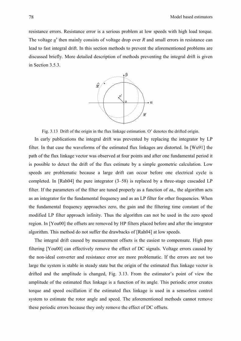
Model based estimators 78
resistance errors. Resistance error is a serious problem at low speeds with high load torque.
The voltage us then mainly consists of voltage drop over R and small errors in resistance can
lead to fast integral drift. In this section methods to prevent the aforementioned problems are
discussed briefly. More detailed description of methods preventing the integral drift is given
in Section 3.5.3.
α
β
o'o
ψ
ψ
Fig. 3.13 Drift of the origin in the flux linkage estimation. O’ denotes the drifted origin.
In early publications the integral drift was prevented by replacing the integrator by LP
filter. In that case the waveforms of the estimated flux linkages are distorted. In [Wu91] the
path of the flux linkage vector was observed at four points and after one fundamental period it
is possible to detect the drift of the flux estimate by a simple geometric calculation. Low
speeds are problematic because a large drift can occur before one electrical cycle is
completed. In [Rah04] the pure integrator (3–58) is replaced by a three-stage cascaded LP
filter. If the parameters of the filter are tuned properly as a function of ω r , the algorithm acts
as an integrator for the fundamental frequency and as an LP filter for other frequencies. When
the fundamental frequency approaches zero, the gain and the filtering time constant of the
modified LP filter approach infinity. Thus the algorithm can not be used in the zero speed
region. In [You00] the offsets are removed by HP filters placed before and after the integrator
algorithm. This method do not suffer the drawbacks of [Rah04] at low speeds.
The integral drift caused by measurement offsets is the easiest to compensate. High pass
filtering [You00] can effectively remove the effect of DC signals. Voltage errors caused by
the non-ideal converter and resistance error are more problematic. If the errors are not too
large the system is stable in steady state but the origin of the estimated flux linkage vector is
drifted and the amplitude is changed, Fig. 3.13. From the estimator’s point of view the
amplitude of the estimated flux linkage is a function of its angle. This periodic error creates
torque and speed oscillation if the estimated flux linkage is used in a sensorless control
system to estimate the rotor angle and speed. The aforementioned methods cannot remove
these periodic errors because they only remove the effect of DC offsets.
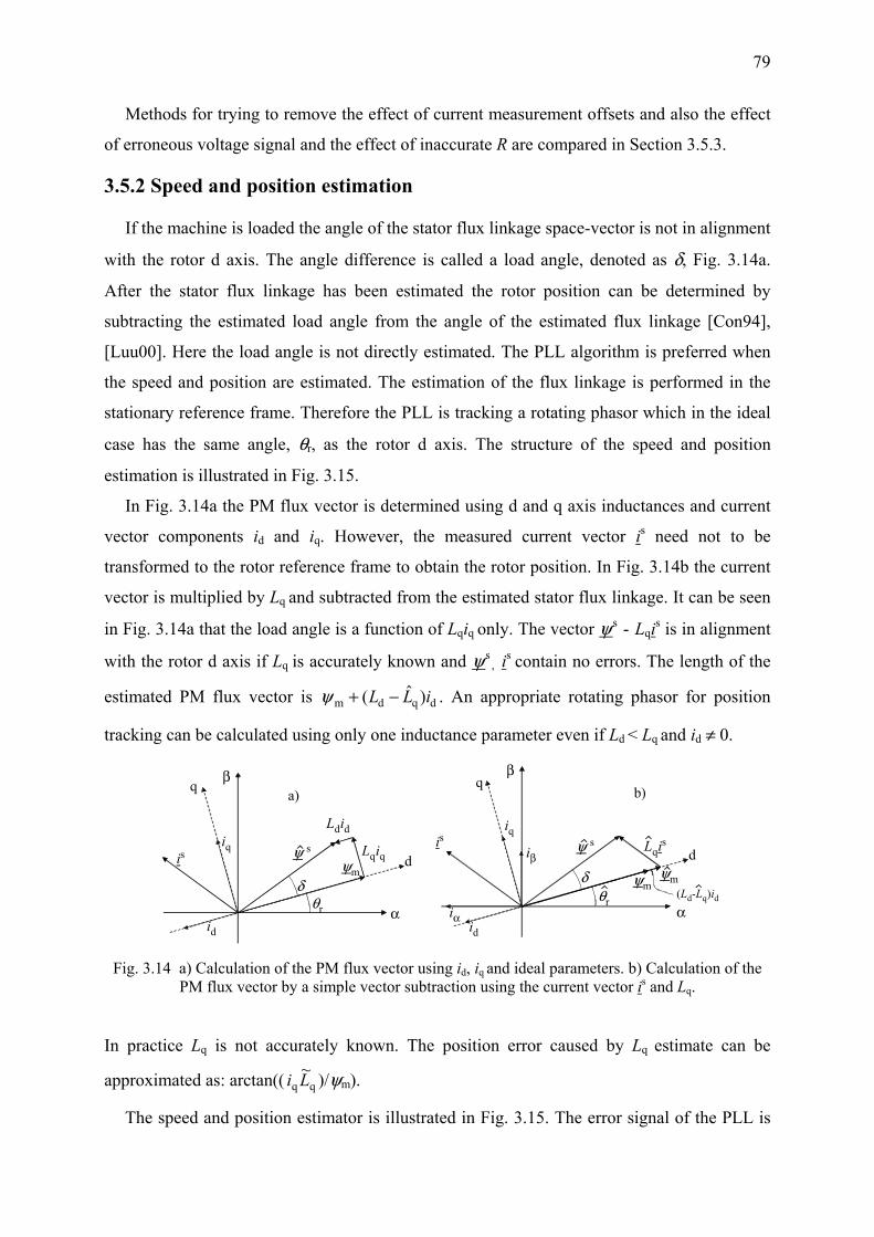
79
Methods for trying to remove the effect of current measurement offsets and also the effect
of erroneous voltage signal and the effect of inaccurate R are compared in Section 3.5.3.
3.5.2 Speed and position estimation
If the machine is loaded the angle of the stator flux linkage space-vector is not in alignment
with the rotor d axis. The angle difference is called a load angle, denoted as δ, Fig. 3.14a.
After the stator flux linkage has been estimated the rotor position can be determined by
subtracting the estimated load angle from the angle of the estimated flux linkage [Con94],
[Luu00]. Here the load angle is not directly estimated. The PLL algorithm is preferred when
the speed and position are estimated. The estimation of the flux linkage is performed in the
stationary reference frame. Therefore the PLL is tracking a rotating phasor which in the ideal
case has the same angle, θr, as the rotor d axis. The structure of the speed and position
estimation is illustrated in Fig. 3.15.
In Fig. 3.14a the PM flux vector is determined using d and q axis inductances and current
vector components id and iq. However, the measured current vector is need not to be
transformed to the rotor reference frame to obtain the rotor position. In Fig. 3.14b the current
vector is multiplied by Lq and subtracted from the estimated stator flux linkage. It can be seen
in Fig. 3.14a that the load angle is a function of Lqiq only. The vector ψ s - Lqis is in alignment
with the rotor d axis if Lq is accurately known and ψ s, is contain no errors. The length of the
estimated PM flux vector is dqdm )ˆ( iLL −+ψ . An appropriate rotating phasor for position
tracking can be calculated using only one inductance parameter even if Ld < Lq and id ≠ 0.
d
α
β
ψm
q
ψ s Lqiq
θr
δ
iq
id
Ldid
d
α
β
ψm
q
is
θr
a) b)
isψ s
iα
iβψm
Lqis
(Ld-Lq)id
id
iq
δ
Fig. 3.14 a) Calculation of the PM flux vector using id, iq and ideal parameters. b) Calculation of the
PM flux vector by a simple vector subtraction using the current vector is and Lq.
In practice Lq is not accurately known. The position error caused by Lq estimate can be
approximated as: arctan(( qq~Li )/ψm).
The speed and position estimator is illustrated in Fig. 3.15. The error signal of the PLL is

Model based estimators 80
the difference between the angle of the estimated PM flux vector and the estimated rotor
position. This operation requires one arctan operation. An other method is to form a rotating
complex phasor using the sine and cosine of the estimated θr. In that case the error signal εd
would be a cross product: rmrmβˆsinˆcos θψθψ α− .
I
εd ωr
θr
Ik1
k2 +
uref
isflux linkageestimator
++-
-
Lqiα
ψα
ψβ
ψmα
ψmβarg +
−θr
PLL
Lqiβ
s
Fig. 3.15 Speed and position estimator. The input of the PLL is the angle difference between the
estimated PM flux vector and the position output of the PLL.
3.5.3 Drift correction methods
In Sections 3.5.3.1 and 3.5.3.2 the flux linkage is estimated using only the voltage model,
(3–58). These methods need the inductance information only when the rotor position is
estimated, Fig. 3.15. Section 3.5.3.3 deals with estimators where the integral drift is prevented
using a current model. The current model estimates the same flux linkage as (3–58) using PM
flux information and flux linkage components Ldid and Lqiq.
3.5.3.1 Hu & Wu method, modified integrator
The modified integrator presented in [Hu98] is a well known method to prevent problems
of the flux linkage estimation. If the amplitude of the estimated flux linkage exceeds the limit
value the algorithm acts as an LP filter. Otherwise the algorithm is a pure integrator. The
transfer function of the modified integrator is
)()(1)(c
c
csz
ssx
ssy
ωω
ω ++
+= (3–59)
The algorithm is illustrated in Fig. 3.16. If y exceeds limit L, z = L, otherwise z = y.
+s + ωc
+1
s + ωc
ωc
Lz
yx
Fig. 3.16 Modified integrator with a saturable feedback.
The problem of the algorithm in Fig. 3.16 is the proper selection of the limiting constant L.

81
A wrong limit value distorts the estimated flux. In [Hu98] an improved algorithm is
introduced which is suitable for AC drives where the flux linkage is not constant. The
improved method exploits the fact that the flux linkage and its back-emf are orthogonal. If a
drift occurs this orthogonal relation is lost and can be detected from non-zero scalar product
between the flux linkage estimate and its back-emf, Fig. 3.17. The scalar product is divided
by the amplitude of the estimated flux linkage and it is amplified by the PI controller.
uα,ref −Riα
1s + ωc ωc
s + ωcPI
polartocartesian
cartesiantopolar
uβ,ref −Riβ
ψαeα + ψβeβ ψα
ψβ1s + ωc
ωcs + ωc
+ +
+
+
ψ
flux angle
Fig. 3.17 Modified algorithm with adaptive flux linkage limit [Hu98].
PI controller output is the compensation signal amplitude suitable for the present flux linkage
value.
Compared to many other drift correction methods the basic structure of the improved
Hu&Wu algorithm, Fig. 3.17, is rather complex. In [Luu00] the structure is simplified by
limiting the flux linkage amplitude directly in the cartesian coordinates. In that case the
trigonometric operations are not needed.
In [Nie99] the drift of the flux linkage estimate is prevented by using a simpler algorithm.
Hu&Wu algorithm and [Nie99] are compared in [Luu00]. Performance of the algorithm
presented in [Nie99] is better. This simple method is studied in the next section. Hu&Wu
algorithm is not further discussed here.
3.5.3.2 Niemelä estimator
It is easy to see from Fig. 3.13 that the maximum value of the flux linkage estimate is
achieved in the direction of the drifted origin. The drift is detected by monitoring the modulus
of the estimated flux linkage vector, |ψ|2 = ψα2+ψβ
2, Fig. 3.18. The average is removed by
subtracting the modulus from its LP filtered value and the result is denoted as ε. It was shown
in [Nie99] that the direction of the drifted origin is approximately the same as the direction of
the flux linkage estimate when ε is at maximum. ε is amplified by a gain g and multiplied by
the flux linkage estimate. The result is a correction vector which is added to the integration
algorithm (3–58). Now the integral of us – Ris can be written in discrete form:
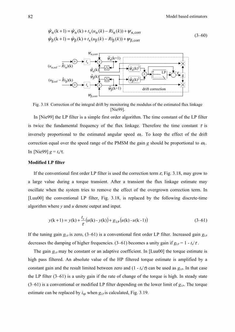
Model based estimators 82
corrβ,ββsββ
corrα,ααsαα
))()(()k(ˆ)1k(ˆ))()(()k(ˆ)1k(ˆ
ψψψψψψ
+−+=+
+−+=+
kRikut
kRikut (3–60)
(uα,ref − Riα)(k)ts +
ψα(k+1)
ψα(k)
ts +ψβ(k+1)
ψβ(k)(uβ,ref − Riβ)(k)
drift correction
+
+
−+ g
ψα(k)2
ψβ(k)2+ LP ε
ψα,corr
ψβ,corr Fig. 3.18 Correction of the integral drift by monitoring the modulus of the estimated flux linkage
[Nie99].
In [Nie99] the LP filter is a simple first order algorithm. The time constant of the LP filter
is twice the fundamental frequency of the flux linkage. Therefore the time constant τ is
inversely proportional to the estimated angular speed ω r . To keep the effect of the drift
correction equal over the speed range of the PMSM the gain g should be proportional to ω r .
In [Nie99] g = ts/τ.
Modified LP filter
If the conventional first order LP filter is used the correction term ε, Fig. 3.18, may grow to
a large value during a torque transient. After a transient the flux linkage estimate may
oscillate when the system tries to remove the effect of the overgrown correction term. In
[Luu00] the conventional LP filter, Fig. 3.18, is replaced by the following discrete-time
algorithm where y and u denote output and input.
( ) ( )1)-(k-(k)(k)-(k)(k)1)(k LPs uugyu
tyy ++=+
τ (3–61)
If the tuning gain gLP is zero, (3–61) is a conventional first order LP filter. Increased gain gLP
decreases the damping of higher frequencies. (3–61) becomes a unity gain if gLP = 1 - ts/τ .
The gain gLP may be constant or an adaptive coefficient. In [Luu00] the torque estimate is
high pass filtered. An absolute value of the HP filtered torque estimate is amplified by a
constant gain and the result limited between zero and (1 - ts/τ) can be used as gLP. In that case
the LP filter (3–61) is a unity gain if the rate of change of the torque is high. In steady state
(3–61) is a conventional or modified LP filter depending on the lower limit of gLP. The torque
estimate can be replaced by iqe when gLP is calculated, Fig. 3.19.

83
HPiqe ABS gadapt gLP
Fig. 3.19 Adaptive calculation of gLP.
The modified LP filter decreases unnecessary large flux linkage corrections when the
torque changes rapidly. If the gain gLP is adaptive it is possible to completely disable the
correction of the flux linkage estimate during torque steps.
In DTC drive this modification clearly improves the performance of the estimator [Luu00].
It also increases the number of the tuning parameters. The filtering time constant of the first
order HP filter and the gain gadapt must be appropriately selected.
3.5.3.3 Effect of parameter errors
The stator resistance is the only parameter needed in the flux linkage estimation, Fig. 3.18.
In Fig. 3.20 the error between the actual input vector ( ss iRu − ) and the input of the estimator
( ss ˆiRu − ) is drawn in steady state. The drift is removed. It can be calculated from Fig. 3.20
that the angle error χ between vectors ss iRu − and ss ˆiRu − is
χ = ⎟⎠⎞⎜
⎝⎛ −− )cos~/()sin~(arctan ssss υυ iRiRuiR (3–62)
where υ = ϕ + arctan( (|Ris|sinϕ ) / (|u| – |Ris|cosϕ) ), ϕ is an angle between the stator voltage
and current vectors and RRR ˆ~ −= .
α
β
is
usRis
Ris
ϕus-Ris
u s-R i sυ
χ
Fig. 3.20 Input error of the flux linkage estimator.
The amplitude of ss ˆiRu − is
2s2sssss sin~cos~ˆ ⎟⎠⎞⎜
⎝⎛+⎟
⎠⎞⎜
⎝⎛ −−=− υυ iRiRiRuiRu (3–63)
υ is usually rather small in PMSMs because no magnetizing current is needed. Therefore

Model based estimators 84
angle error (3–62) is small and the amplitude difference ssss ˆiRuiRu −−− ≈ s~ iR . After
integration of the voltage error vector | ss iRu − | - | ss ˆiRu − | the angle of the flux error vector
is (3–62) but the amplitude difference (3–63) is divided by ω r .
rs /~ˆ ωψψ iR≈− (3–64)
3.5.3.3 Methods exploiting the current model
Some flux estimators also exploit the flux linkage information of so-called current model
to prevent drift problems. In the literature a non-salient machine is often assumed. The stator
flux linkage of the PMSM can be written:
βrmcβ,
αrmcα,
ˆˆsinˆˆ
ˆˆcosˆˆ
iL
iL
+=
+=
θψψ
θψψ (3–65)
If this assumption is not done the flux linkage in the stationary reference frame is [And99]:
rqqrddmcβ,
rqqrddmcα,
ˆcosˆˆsin)ˆˆ(ˆ
ˆsinˆˆcos)ˆˆ(ˆ
θθψψ
θθψψ
iLiL
iLiL
++=
−+= (3–66)
In [Fre96] the flux linkage is estimated by an algorithm which uses three-phase equations.
This method also inherently estimates the rotor position. In the case of the voltage model
methods discussed above the rotor position must be determined by an additional algorithm.
However, the structure of [Fre96] is complicated compared to voltage model algorithms. In
[Öst96] the structure of [Fre96] is simplified by using a space-vector presentation.
In [And99] the position is estimated and the drift is eliminated by comparing the voltage
and current models, (3–58) and (3–66). This type of estimator is called a model reference
adaptive system (MRAS). The angle difference between the flux linkage space-vectors
(ψ c , ψu) is used as an error signal for the PLL algorithm which calculates the position and
speed estimates. The current model is corrected using the estimated position rθ . Therefore the
current model is called an adaptive model. Voltage model is called a reference model.
The drift is corrected by adding a correction vector ucorr to the integrator input us-Ris, Fig.
3.21. ucorr is achieved by amplifying α and β components of (ψc - ψu) by PI controller. The
structure of the algorithm is fairly simple, but due to the drift correction the voltage model is
coupled with the position estimate, Fig. 3.21. Voltage model flux estimators, Fig. 3.17 and
Fig. 3.18, do not need position information.

85
ψde=ψm+Ldide
ψuα= (uα- Riα+ ucorr,α)dt
ψuβ = (uβ- Riβ+ ucorr,β)dt ψu
ψc
ψu ψiIPI
θrωr
is
us
pos.error
PI+−
ucorr correction vector
θr
e-jθ ejθψqe=Lqiqe
ire ψcre
Fig. 3.21 Block diagram of the MRAS estimator with drift correction [And99].
[And99] was compared to the stationary frame version of [Mat90] by the author in [Esk03].
The low speed performance of Matsui’s back-emf method was superior.
Also new approaches are published recently. In [Pii05] an interesting adaptive estimator is
introduced where the estimation is performed in the estimated d,q frame instead of stationary
frame. Now the reference model is the current model
qeqcqe
dedmcdeˆˆ
iLiL
=+=
ψψψ
(3–67)
The adaptive model for flux linkage is the basic voltage equation (3–32) in the d,q frame
( )( )dtiRiu
dtiRiu
∫
∫
+−−=
++−=
qeuderqeqeuqe
deuqerdedeude~kˆˆˆ
~kˆˆˆ
ψωψ
ψωψ (3–68)
where k is a constant gain. The estimated speed is the parameter used to adjust the adaptive
model in a manner which minimises the error between the adaptive and the reference model
(3–67). The adaptive model also calcultates an estimate for the current:
quqeqedmudede /ˆˆ,/)ˆ(ˆ LiLi ψψψ =−= . These current components are subtracted from ide
and iqe and the error is used to correct the voltage model (3–68). The block diagram of the
estimator is presented below.

Model based estimators 86
ψu= (ure-Rire-jωrψ re+ki re)
(ψude-ψm)/Ldψuqe/Lq
adaptive model
ψcde=ψm+Ldideψcqe=Lqiqe
+−
reference model
ωr
Ik1
k2 +
PI-controller
ψuqe
ψcqe
ure
+i re-
ire
Fig. 3.22 Adaptive estimator in the estimated rotor reference frame, [Pii05].
In [Pii05] the model based method was assisted with a signal injection estimator. The
result is a hybrid estimator which is stable also at zero speed region. This type of estimators
are discussed in Chapter 4. Unfortunately, [Pii05] is not compared to other model based
estimators in this study because it was published after the comparative study was completed.
Rasmussen estimator
In [Ras03] the drift of the flux linkage estimate is prevented by a simple scheme based on
the current model. The block diagram of the discrete time algorithm is illustrated in Fig. 3.23.
The flux linkage components Lqiα and Lqiβ are subtracted from the flux linkage estimated by
the voltage model. The remaining vector represents the PM flux linkage in stationary
reference frame. In [Ras03] a non-salient machine is assumed. Here the PM flux linkage is
estimated using Lq of a salient machine. The estimated scalar ψm is subtracted from the length
of the calculated PM flux linkage. If drift occurs the difference is nonzero. PM flux error is
multiplied by gain g and transformed to the stationary reference frame. The resulting
correction terms uα,corr and uβ,corr are added to the inputs of the integral algorithm. Now the
rotor position estimation is included in the drift correction scheme, Fig. 3.23. This estimate
can be directly used as an input for the PLL estimating the rotor speed and position, Fig. 3.15.
(uα,ref − Riα)(k)ts +
ψα(k+1)
+−
ψα(k)
ts +ψβ(k+1)
ψβ(k)
ψm
uα,corr(k)
(uβ,ref − Riβ)(k)
drift correction
+
+ −+
Lqiα(k)
Lqiβ(k)
−+
ψmecosθr
ψmesinθr |ψme| e jθ
arg(ψme)θr
g
uβ,corr(k)
Fig. 3.23 Correction of the integral drift by estimating the permanent magnet flux [Ras03].

87
Parameter sensitivity of Rasmussen method
The effect of PM flux error was analysed in [Ras03]. The following analysis also contains
the resistance and inductance error. As discussed in Section 3.5.2 the rotor position can be
accurately calculated in the stationary reference frame using the current vector and one
inductance parameter, Fig. 3.14. However, the estimated length of the PM flux vector, Fig.
3.23, is not correct if Ld < Lq and id ≠ 0. Therefore it is important to notice that the effect of the
inductance error in the parameter sensitivity analysis below is valid only if the machine is
non-salient or id is very small.
The estimated and real stator flux linkage derivatives can be written on the basis of Fig.
3.23 as follows
( ) rr ˆmem
sssq
ˆme
s )ˆ(ˆˆˆ θθ ψψψψ jj egiRuiLedtd
dtd −+−=+= (3–69)
( ) sssqm
s r iRuiLedtd
dtd j −=+= θψψ (3–70)
where ψme is the length of the PM flux vector estimated by the algorithm, Fig. 3.23. rθ is the
angle of the estimated PM vector ψme and also the estimated rotor position. Steady state
operation is assumed: rrr //ˆ ωθθ == dtddtd . When (3–70) is subtracted from (3–69) and the
result is transformed to estimated synchronous reference frame with angle rθ , the result is:
( ) ( ) )ˆ(~~ˆˆ memrere
q
~
mmerrere r ψψψψωψψ θ −+=−−⎟
⎠⎞
⎜⎝⎛ +=− giRiLej
dtd
dtd j (3–71)
A small position error is assumed. Thus 1~cos r ≈θ and θθ ~~sin r ≈ . Let us denote:
X = (ψme - ψm)/ ψm and Y = ( mmm /)ˆ ψψψ − . Real and imaginary parts of (3–71) are
mqm
qqede
m
qrrr
mderrqem
qr
m
de
/~~~
ˆ/~ˆ:Im
/~~ˆ~
ˆ~
/:Re
ψψψ
ωθω
ψθωψ
ωψ
iRL
dtdi
iL
dtdX
gYiRgXiLL
dtdi
dtdX
=−−−
+=+++− (3–72)
Components containing current derivatives or ide are assumed to be zero. When the derivative
operator is replaced by a Laplace operator s the position error is

Model based estimators 88
)()ˆ(
~ˆ~)()(
ˆˆ
)(~q
m2r
2q
2r
2r
2r
r sigss
LRgssY
gssgs
ψωω
ωωθ
++
++−
++= (3–73)
The steady state position error is approximately
qeq2rmmr
mmr
~ˆ
~1ˆ
)ˆ(~ iLRgg⎟⎟⎠
⎞⎜⎜⎝
⎛+−
−≈
ωψψωψψθ (3–74)
A low tuning parameter g produces a lower position error but the dynamic performance is
impaired.
3.6 Comparison of the model based estimators by simulations
In this section Matsui’s back-emf estimators are compared to flux linkage estimators in
simulations. The simulations are carried out using Matlab Simulink program. The vector
control system, Fig. 2.25, and speed & position estimators are modelled using the S-function
property. S-function contains a text file where the discrete time algorithms are written using
some common programming language. In this thesis Matlab’s own language is used. The
PMSM is modelled in the rotor reference frame using time continuous Simulink blocks. The
model is presented in Fig. 3.24. It contains also the 6th harmonic of the inductance and the
rotor flux linkage (2-22).
3.6.1 Simulations with ideal PMSM drive
In the first stage the frequency converter is assumed to be ideal. The stator voltage of the
model is the voltage reference vector and the current measurement contains no errors. The
PMSM model contains only the fundamental frequency components (Ld, Lq and ψm are
constants). In Fig. 3.24 coefficients L6 (L6 in (2-22)) and PM6 (ψmd6, ψmq6 in (2-22)) are set at
zero. The parameters of the motor model and estimator algorithms are varied to compare the
sensitivity for parameter errors.
Back-emf estimators (Matsui’s methods) are modelled in synchronous reference frame and
flux linkage estimators (Niemelä and Rasmussen methods) in stationary frame. The control
system in rotor frame is illustrated in Fig. 2.25 and the counterpart in the stationary frame in
Fig. 2.26. The discrete algorithm of the PI controllers is presented in Fig. 2.27. The control
system parameters, Table 3.1, are similar in all simulations. The control and estimator
algorithms are performed in 100 µs loop, which is also the calculation time of the
experimental setup.

89
Table. 3.1 Parameters of the control system used in simulations.
Gain kp Integration time ti
Speed control 2 0.033 s Current control 20 0.005 s
The PMSM used in simulations is a 3.5 kW 1500 rpm machine with surface mounted
magnets. The number of pole pairs is 3. More detailed information is provided in
Appendix A. With the parameters of the machine and Table 3.1 the closed loop bandwidth of
the current control is approximately 300 Hz. The speed control bandwidth is approximately
60 Hz in the case of measured speed and position. The closed loop bandwidth is the frequency
when the output is attenuated 3 dB compared to the sinusoidal reference value.
Fig. 3.24 Simulink model of the PMSM in the rotor reference frame.
The selected model based estimators are compared using the test sequence presented in
Fig. 3.25. The load torque is nominal (22 Nm) and positive for 0 - 2.5 s. The speed reference
signal is -1 p.u. during the first 0.5 s and the PMSM is then generating. For 0.5 - 1.5 s the
speed reference is 1 p.u. and the PMSM power flows from the supply to the motor. At 1.5 s
the speed reference is changed to 0.1. The direction of the rotation is changed at 2 s. The load

Model based estimators 90
torque is changed from 100% to -100 % value at 2.5 s. In the last stage the PMSM is
accelerated from speed -0.1 p.u. to speed 0.45 p.u. Per unit (p.u.) values are used throughout
this study when simulated or measured rotor speeds are shown. 1 p.u. is the nominal speed
given by the manufacturer. Nominal values of the PMSMs and per unit values for the
parameters are given in Appendix A.
In all simulations the current was limited to 22 A which is approximately twice the
nominal value. The simulation results presented in the following sections were obtained with
nominal load. All simulations are also carried out without load and with medium load. The
undesirable effects of the non-ideal PMSM drive and parameter errors are more serious in the
case of nominal load. Therefore small load simulations are not presented.
Fig. 3.25 The simulation sequence for comparing the parameter sensitivity of estimators.
3.6.1.1 Back-emf estimators
The tuning parameters of the back-emf estimators are presented in Table 3.2. In [Mat96],
[Nah04] d axis correction gain k2 was constant. However, the d axis total gain is proportional
to speed (3–49), Fig. 3.11. If k2 is suitable for a low speed range the total gain may become
excessive around the nominal speed and the system is subjected to noise. In this thesis k2 is
linearly decreased when the rotor speed is over 0.15 p.u.
Table. 3.2 Tuning parameters of back-emf estimators.
ρ (3–38) ω low (3–38) k1 k2 “voltage model” (Fig. 3.6) 80/s 0.2 p.u. (94.2 rad/s) – –
“current model” (Fig. 3.10) – – 120 if (|ω r |< 0.15 p.u), k2 = 280
else, k2 = 280-188*(ω r (p.u)-0.15)Combined method
(Fig. 3.12) 80/s 0.2 p.u. (94.2 rad/s) 120 –
The tuning of the PI controller of the PLL of Matsui’s “voltage model” estimator is
presented in (3–38). The selection ρ = 80/s gives a rather narrow bandwidth (≈ 32 Hz) for the
PLL. The narrow bandwidth is allowed because the speed is estimated mainly by the q axis
branch, Fig. 3.6. The gain k1 defines the bandwidth of the LP filter type direct speed estimator
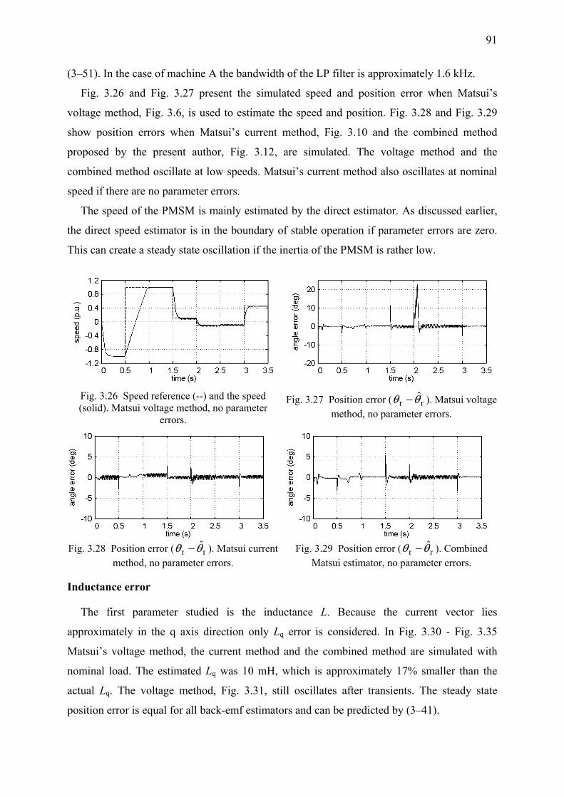
91
(3–51). In the case of machine A the bandwidth of the LP filter is approximately 1.6 kHz.
Fig. 3.26 and Fig. 3.27 present the simulated speed and position error when Matsui’s
voltage method, Fig. 3.6, is used to estimate the speed and position. Fig. 3.28 and Fig. 3.29
show position errors when Matsui’s current method, Fig. 3.10 and the combined method
proposed by the present author, Fig. 3.12, are simulated. The voltage method and the
combined method oscillate at low speeds. Matsui’s current method also oscillates at nominal
speed if there are no parameter errors.
The speed of the PMSM is mainly estimated by the direct estimator. As discussed earlier,
the direct speed estimator is in the boundary of stable operation if parameter errors are zero.
This can create a steady state oscillation if the inertia of the PMSM is rather low.
Fig. 3.26 Speed reference (--) and the speed (solid). Matsui voltage method, no parameter
errors.
Fig. 3.27 Position error ( rr θθ − ). Matsui voltage method, no parameter errors.
Fig. 3.28 Position error ( rr θθ − ). Matsui current
method, no parameter errors. Fig. 3.29 Position error ( rr θθ − ). Combined
Matsui estimator, no parameter errors.
Inductance error
The first parameter studied is the inductance L. Because the current vector lies
approximately in the q axis direction only Lq error is considered. In Fig. 3.30 - Fig. 3.35
Matsui’s voltage method, the current method and the combined method are simulated with
nominal load. The estimated Lq was 10 mH, which is approximately 17% smaller than the
actual Lq. The voltage method, Fig. 3.31, still oscillates after transients. The steady state
position error is equal for all back-emf estimators and can be predicted by (3–41).
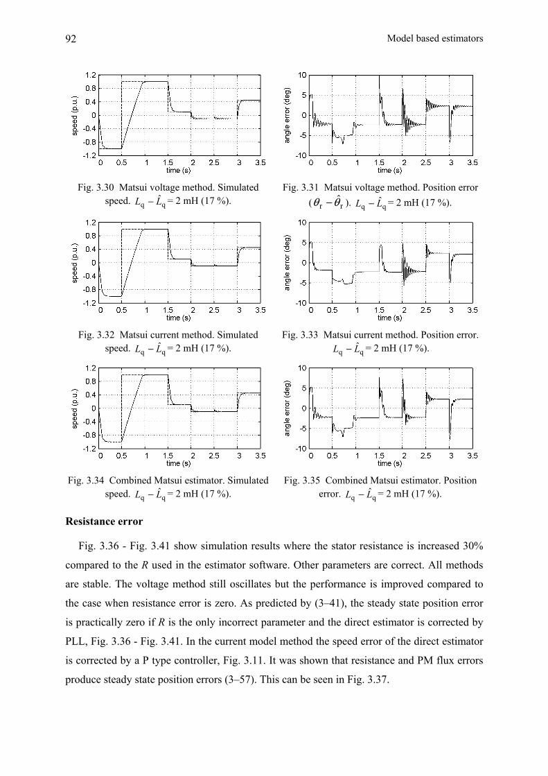
Model based estimators 92
Fig. 3.30 Matsui voltage method. Simulated
speed. qq LL − = 2 mH (17 %). Fig. 3.31 Matsui voltage method. Position error
( rr θθ − ). qq LL − = 2 mH (17 %).
Fig. 3.32 Matsui current method. Simulated
speed. qq LL − = 2 mH (17 %). Fig. 3.33 Matsui current method. Position error.
qq LL − = 2 mH (17 %).
Fig. 3.34 Combined Matsui estimator. Simulated
speed. qq LL − = 2 mH (17 %). Fig. 3.35 Combined Matsui estimator. Position
error. qq LL − = 2 mH (17 %).
Resistance error
Fig. 3.36 - Fig. 3.41 show simulation results where the stator resistance is increased 30%
compared to the R used in the estimator software. Other parameters are correct. All methods
are stable. The voltage method still oscillates but the performance is improved compared to
the case when resistance error is zero. As predicted by (3–41), the steady state position error
is practically zero if R is the only incorrect parameter and the direct estimator is corrected by
PLL, Fig. 3.36 - Fig. 3.41. In the current model method the speed error of the direct estimator
is corrected by a P type controller, Fig. 3.11. It was shown that resistance and PM flux errors
produce steady state position errors (3–57). This can be seen in Fig. 3.37.

93
Fig. 3.36 Matsui current method. Simulated
speed. RR ˆ− = 0.3 Ω (30%). Fig. 3.37 Matsui current method, position error
( rr θθ − ). RR ˆ− = 0.3 Ω (30%).
Fig. 3.38 Matsui voltage method. Simulated
speed. RR ˆ− = 0.3 Ω (30%). Fig. 3.39 Matsui voltage method, position error.
RR ˆ− = 0.3 Ω (30%).
Fig. 3.40 Combined Matsui estimator. Simulated
speed. RR ˆ− = 0.3 Ω (30%). Fig. 3.41 Combined Matsui estimator, position
error. RR ˆ− = 0.3 Ω (30%).
The positive resistance error improves the performance of the sensorless control system
when the PLL type correction algorithms are applied. Steady state position error is practically
zero if the other parameters have correct values. The ringing after transients, Fig. 3.27 - Fig.
3.35, disappears. Very large errors decrease the dynamic performance.
The combined method was tested with 100% resistance error and the system was stable
with nominal load when the test sequence presented above was driven. The maximum
position error was then approximately 40 degrees. If R of the PMSM is 30% smaller than the
R in the software all three back-emf estimators studied are unstable. In that case the PLL
algorithm is not capable of correcting the unstable direct speed estimator.

Model based estimators 94
PM flux error
The flux of the permanent magnets decreases when the temperature of the PMSM rises
[Hen94]. In Fig. 3.42 the combined estimator is simulated in the case when ψm is decreased
by 15% compared to the nominal value, 0.5 Wb. A 15% drop is a large value which requires
that the machine is approximately 100°C warmer than room temperature [Hen94].
Fig. 3.43 shows the position error in the case of the combined method. A rather large error
occurs in the speed reversal but otherwise the effect of positive m~ψ is not significant. The
control system is unstable when Matsui’s original methods are tested with the same error.
If the estimated PM flux is 15% smaller than the actual one the combined Matsui
estimator is unstable. If Lq is also estimated to be too small the performance is improved. The
oscillation in the nominal speed range is damped faster and the maximum position error is
smaller.
Fig. 3.42 Combined Matsui estimator. Simulated
speed. mm ψψ − = -0.075 Wb (-15%). Fig. 3.43 Combined Matsui estimator, position error ( rr θθ − ). mm ψψ − = -0.075 Wb (-15%).
Comparison of back-emf methods
In the simulations presented above Matsui’s voltage method [Mat90] is the poorest of the
three candidates. The position errors after transients are higher compared to other candidates
and the ringing is more intense, Fig. 3.27, Fig. 3.31. The oscillation is caused by the
modelling of the derivative of iq. The derivative algorithm is sensitive to noise and requires
additional LP filtering. This affects the overall dynamic performance.
Matsui’s current model method [Mat92] has a smoother transient performance. The
absence of a PLL type correction algorithm creates greater steady state position errors than
the voltage method, Fig. 3.37.
Matsui’s original algorithms [Mat90], [Mat92] are not further studied by simulations in
this thesis because it is possible to combine most of the positive properties of the Matsui’s
original estimators by using the combined algorithm presented in Fig. 3.12. In the simulations
the combined estimator proved to be less sensitive to parameter errors than [Mat90] and

95
[Mat92]. In the following short list the combined method is compared to the best of Matsui’s
original estimators in each test.
- When the inductance was not correctly estimated the maximum position error of the
combined method was two degrees higher compared to the current method. However, the
oscillation of the combined estimator is attenuated faster, Fig. 3.33, Fig. 3.35.
- In the case of 30% resistance error the maximum position error was approximately seven
degrees smaller than the maximum error in the case of Matsui’s voltage model method Fig.
3.39, Fig. 3.41.
- The proposed combined estimator was stable when the PM flux was decreased by 15%.
Matsui’s original estimators were unstable.
3.6.1.2 Flux linkage estimators
In this Section [Nie99], Fig. 3.18, is compared to the Rasmussen estimator [Ras03], Fig.
3.23. These two methods are selected because they both have a rather simple structure and
they can prevent the drift of the flux linkage estimate caused by parameter errors. The tuning
parameters of the estimators used in the simulations are presented in Table 3.3.
In [Ras03] the gain g was constant. In this thesis g is proportional to rotor speed. This
improves the performance at higher speeds. The correction voltage vector is added to us - Ris,
Fig. 3.23, which is proportional to ω r . Therefore the length of the correction vector is also
proportional to ω r . In the low speed region g is limited to 10.
The tuning of the PLL algorithm is straightforward compared to back-emf methods. The
amplitude of the flux linkage is a function of load torque but can be considered a constant.
Therefore the PLL tuning coefficients can be constant over the speed range. PLL can be tuned
fast compared to back-emf estimators. The bandwidth of the PLL is approximately 300 Hz.
Thus the dynamic performance of the estimator is mainly dependent on the flux linkage
estimator.
Table. 3.3 Tuning parameters of flux linkage estimators.
τ (time constant of LP filter) g PLL (Fig. 3.3a)
Niemelä estimator 2/ω r ts/τ (low limit 0.001) k1 = 3000^2, k2 = 6000
Rasmussen estimator – ω r /1.5 (low limit 10) k1 = 3000^2, k2 = 6000
Simulations without parameter errors
In Fig. 3.44 - Fig. 3.45 the Niemelä method is simulated without parameter errors. In Fig.
3.46 - Fig. 3.49 the same simulation is carried out with the modified Niemelä estimator and
with Rasmussen method. In the modified Niemelä estimator the filtering time constant of the

Model based estimators 96
HP filter, is 0.5 ms and the gain gadapt is 4, Fig. 3.19. These parameters are used in the
following simulations.
Niemelä method oscillates as the back-emf estimators in the previous section. If the
modified LP filter is used the performance is clearly improved, Fig. 3.47. The Rasmussen
estimator has no problems with accurate parameters.
It can be seen in Fig. 3.45, Fig. 3.47 and Fig. 3.49 that there is a position error even if the
parameters are accurately known. The flux linkage estimators are performed in the stationary
reference frame. The steady state position error is created by the computation delays.
Fig. 3.44 Niemelä estimator. No parameter errors.
Simulated speed. Fig. 3.45 Niemelä estimator. No parameter errors.
Position error ( rr θθ − ).
Fig. 3.46 Modified Niemelä estimator. No
parameter errors. Simulated speed. Fig. 3.47 Modified Niemelä estimator. No parameter errors. Position error ( rr θθ − ).
Fig. 3.48 Rasmussen estimator. No parameter
errors. Simulated speed. Fig. 3.49 Rasmussen estimator. No parameter
errors. Position error ( rr θθ − ).
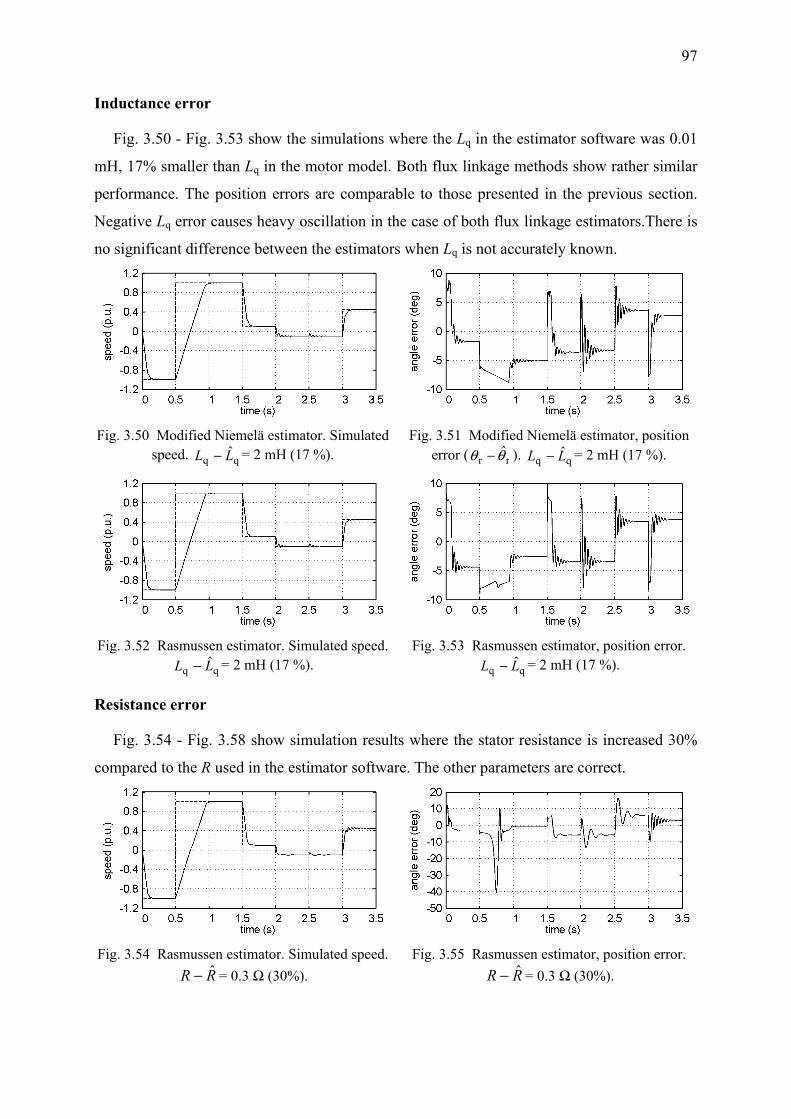
97
Inductance error
Fig. 3.50 - Fig. 3.53 show the simulations where the Lq in the estimator software was 0.01
mH, 17% smaller than Lq in the motor model. Both flux linkage methods show rather similar
performance. The position errors are comparable to those presented in the previous section.
Negative Lq error causes heavy oscillation in the case of both flux linkage estimators.There is
no significant difference between the estimators when Lq is not accurately known.
Fig. 3.50 Modified Niemelä estimator. Simulated
speed. qq LL − = 2 mH (17 %). Fig. 3.51 Modified Niemelä estimator, position
error ( rr θθ − ). qq LL − = 2 mH (17 %).
Fig. 3.52 Rasmussen estimator. Simulated speed.
qq LL − = 2 mH (17 %). Fig. 3.53 Rasmussen estimator, position error.
qq LL − = 2 mH (17 %).
Resistance error
Fig. 3.54 - Fig. 3.58 show simulation results where the stator resistance is increased 30%
compared to the R used in the estimator software. The other parameters are correct.
Fig. 3.54 Rasmussen estimator. Simulated speed.
RR ˆ− = 0.3 Ω (30%). Fig. 3.55 Rasmussen estimator, position error.
RR ˆ− = 0.3 Ω (30%).

Model based estimators 98
Fig. 3.56 Modified Niemelä estimator. Simulated
speed. RR ˆ− = 0.3 Ω (30%). Fig. 3.57 Modified Niemelä estimator, position
error. RR ˆ− = 0.3 Ω (30%).
Fig. 3.58 Niemelä estimator (basic algorithm), position error. RR ˆ− = 0.3 Ω (30%).
The Rasmussen method is stable, but position errors are large compared to back-emf
methods. There are also steady state position errors at low speeds, Fig. 3.55. This can be
predicted by (3–74).
The modified Niemelä estimator oscillates after the speed is reversed from 0.1 p.u. speed
to -0.1 p.u. and in the end of the simulation period. In the case of the 30% resistance error
there is no significant difference between the original [Nie99] and the modified estimator,
Fig. 3.57, Fig. 3.58. Both Rasmussen and Niemelä methods are unstable in the low speed
region if the estimated resistance is 30% larger than the actual one.
PM flux error
PM flux error is tested only in the case of the Rasmussen estimator because ψm need not to
be known if [Nie99] is applied. In Fig. 3.59 and Fig. 3.60 the flux of the permanent magnets
is decreased by 15%. Simulator software uses the nominal value 0.5 Wb. In Fig. 3.61 and Fig.
3.62 ψm of the motor model is 0.5 Wb and mψ = 0.425 Wb. The Rasmussen estimator is not
sensitive to the PM flux error.
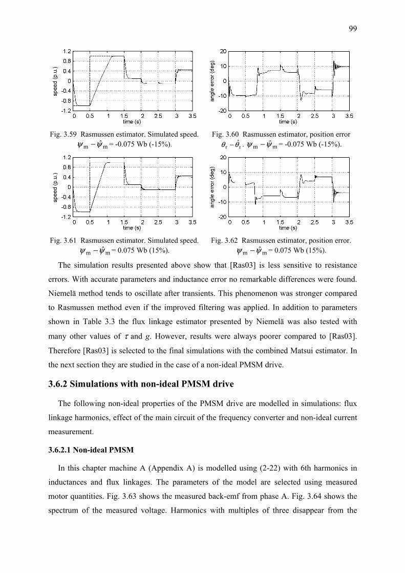
99
Fig. 3.59 Rasmussen estimator. Simulated speed.
mm ψψ − = -0.075 Wb (-15%). Fig. 3.60 Rasmussen estimator, position error
rr θθ − . mm ψψ − = -0.075 Wb (-15%).
Fig. 3.61 Rasmussen estimator. Simulated speed.
mm ψψ − = 0.075 Wb (15%). Fig. 3.62 Rasmussen estimator, position error.
mm ψψ − = 0.075 Wb (15%).
The simulation results presented above show that [Ras03] is less sensitive to resistance
errors. With accurate parameters and inductance error no remarkable differences were found.
Niemelä method tends to oscillate after transients. This phenomenon was stronger compared
to Rasmussen method even if the improved filtering was applied. In addition to parameters
shown in Table 3.3 the flux linkage estimator presented by Niemelä was also tested with
many other values of τ and g. However, results were always poorer compared to [Ras03].
Therefore [Ras03] is selected to the final simulations with the combined Matsui estimator. In
the next section they are studied in the case of a non-ideal PMSM drive.
3.6.2 Simulations with non-ideal PMSM drive
The following non-ideal properties of the PMSM drive are modelled in simulations: flux
linkage harmonics, effect of the main circuit of the frequency converter and non-ideal current
measurement.
3.6.2.1 Non-ideal PMSM
In this chapter machine A (Appendix A) is modelled using (2-22) with 6th harmonics in
inductances and flux linkages. The parameters of the model are selected using measured
motor quantities. Fig. 3.63 shows the measured back-emf from phase A. Fig. 3.64 shows the
spectrum of the measured voltage. Harmonics with multiples of three disappear from the

Model based estimators 100
model after transformation to rotor reference frame because they are common for all phases.
The 5th harmonic is approximately 1% of the main rotor flux ψm and the 7th harmonic is
negligible. Using (2-21): ψmd,6 = -ψmq,6 = ψm,5 if ψm,7 = 0. This amplitude of the 6th PM flux
linkage harmonic is denoted as PM6 in the PMSM model, Fig. 3.24. The value of PM6 is
0.005 Wb.
Fig. 3.63 Measured back-emf (phase A) of the PMSM. Mechanical rotor speed is 2000 rpm.
Fig. 3.64 Back-emf spectrum.
Fig. 3.65 Measured phase inductance (phase A)
as a function of the rotor position θ r . Ideal saliency (solid line).
Fig. 3.66 Spectrum of the phase inductance.
Fig. 3.65 shows the measured phase inductance with several rotor positions. Inductance
was measured using the following setup [Vas93]. Phases B and C were connected to the
common point. A sinusoidal 300 Hz voltage signal was generated over this point and phase A.
The device feeding the circuit was a controllable AC voltage source ELGAR SW5250A. The
voltage generated by ELGAR SW5250A and the current of the phase A were measured and
the data was analysed using Matlab. Inductance was determined using the fundamental
frequency components of the voltage and the current. If the rotor d axis is in alignment with
the phase A the measured inductance is Ld. The angle π/2 rad between the rotor d axis and the
phase A gives the quadrature axis inductance Lq.
The spectrum of the saliency curve is illustrated in Fig. 3.66. The first order component is
the main saliency. The second order component, n = 2 in (2-15) and (2-16), is clearly the
dominant harmonic (≈ 11 %). The amplitude of the main saliency (Lq - Ld)/2 is approximately
1.9 mH, Fig. 3.65. Thus L6 (2-22) in the simulation model is 0.2 mH.

101
The effect of a non-ideal PMSM is compared by steady state simulations. The load is
nominal and simulations are performed at 4% speed and 30% speed. Fig. 3.67 shows the
speed and position error when the combined Matsui estimator is studied. The speed reference
signal is set at 4% of nominal speed. The results of at 30% speed are presented in Fig. 3.68. In
Fig. 3.69 and Fig. 3.70 the same simulations are performed with the Rasmussen estimator.
As presented in Chapter 3.5, the steady state position error is greater in the case of the flux
linkage estimator. At speed 0.04 p.u. the peak-to-peak amplitudes of the simulated speed
oscillations are: 0.011 p.u. (Matsui) and 0.019 p.u. (Rasmussen). At speed 0.3 p.u. the
amplitudes are practically the same. The conclusion is that the combined Matsui estimator is
less sensitive to flux linkage harmonics in the low speed region.
Fig. 3.67 Non-ideal PMSM, combined Matsui estimator, full load, 0.04 p.u. speed reference.
a) simulated speed, b) position error.
Fig. 3.68 Non-ideal PMSM, combined Matsui estimator, full load, 0.3 p.u. speed reference.
a) simulated speed, b) position error.
Fig. 3.69 Non-ideal PMSM, Rasmussen, full load, 0.04 p.u. speed reference. a) simulated
speed, b) position error.
Fig. 3.70 Non-ideal PMSM, Rasmussen, full load, 0.3 p.u. speed reference. a) simulated speed,
b) position error.
The speed ripple consisting of multiples of 6th harmonics is clearly damped when the
speed is increased from 0.04 p.u to 0.3 p.u. The frequency of the disturbance is then outside

Model based estimators 102
the closed loop bandwidth of the speed control. If the speed control is tuned faster the low
speed oscillation increases.
3.6.2.2 Effect of the non-ideal frequency converter
The effect of the non-ideal frequency converter is studied by adding an error voltage vector
to the input of the PMSM model, Fig. 3.24. The error voltage vector is the non-linear part of
(2-43). The voltage error equation of the VSI is used because it is the most simple one to
model. The threshold voltage and the effect of dead times are equal to those used in Fig. 2.18.
The amplitude of the error voltage for one phase in the simulations is 1.9 V. In the
simulations of this section the model of the PMSM is ideal.
In Fig. 3.71 the combined Matsui estimator is simulated with 0.04 p.u. speed and nominal
load. Fig. 3.72 presents the steady state simulation at 0.3 p.u. speed. Fig. 3.73 and Fig. 3.74
show the same simulations with the Rasmussen estimator.
The oscillation is stronger when the back-emf estimator is applied, Fig. 3.71. The
amplitude difference can be explained by the structure of the estimators. The voltage
reference vector is a sum of the actual stator voltage and the voltage drop over the
semiconductors of the frequency converter. The voltage drop creates non-linear error voltage
(2-44) which is included in the input of the flux estimator (3–58). The integrator attenuates
the error signal. In the back-emf estimator, where PLL is used to estimate the speed and
position, the effect of the inverter bridge is amplified by the PI controller. In this thesis the
direct amplifier branch of the PI controller does not take part in composing the signal used in
speed control, Fig. 3.6. If the full output of the PI controller is used the transient performance
is improved but the system becomes sensitive to disturbances created by the non-ideal VSI.
Fig. 3.71 Non-ideal VSI, combined Matsui
estimator, Udead+Uth= 1.92 V, full load, 0.04 p.u. speed reference a) speed, b) position error.
Fig. 3.72 Non-ideal VSI, combined Matsui estimator, Udead+Uth= 1.92 V, full load. 0.3 p.u.
speed reference a) speed, b) position error.

103
In the case of the Rasmussen method the voltage error generates an additional position
error in the low speed region, Fig. 3.73. When the back-emf method is simulated the average
steady state position error is not affected by the voltage errors generated by the inverter bridge
Fig. 3.71.
Fig. 3.73 Non-ideal VSI, Rasmussen estimator,
Udead+Uth= 1.92 V, full load, 0.04 p.u. speed reference. a) speed, b) position error.
Fig. 3.74 Non-ideal VSI, Rasmussen estimator, Udead+Uth= 1.92 V, full load, 0.3 p.u. speed
reference. a) speed, b) position error.
3.6.2.3 Effect of non-ideal current measurements
Fig. 3.75 - Fig. 3.78 show simulations where the current measurement of phase A contains
a 0.2 A (≈1.9%) offset. A quantization error of 10 bit A/D conversion is also simulated.
Simulink’s quantizer blocks with 50 mA interval are used. In the simulations of this section
the model of the PMSM is ideal.
The offset creates a speed oscillation at the fundamental frequency [Qia04]. The flux
linkage estimator is more sensitive to the offset error, Fig. 3.75 - Fig. 3.78. Current offset can
be removed by careful tuning of the measurement system. High pass filters can also be used
to remove DC levels.
In Fig. 3.79 - Fig. 3.80 the effect of gain unbalance of current measurement is simulated.
Gain errors create the 2nd harmonic in speed and torque [Qia04]. The current of phase A is
multiplied by 0.95. Other phases have unity gain. The simulations are performed at 0.04 p.u.
speed. The load torque is nominal. The back-emf estimator is slightly more sensitive for gain
unbalance when tuning parameters of Tables 3.2 and 3.3 are used. However, the differences
are not remarkable.

Model based estimators 104
Fig. 3.75 Combined Matsui estimator, current offset 0.2 A in one phase, full load, 0.04 p.u. speed reference. a) speed, b) position error.
Fig. 3.76 Combined Matsui estimator, current offset 0.2 A in one phase, full load, 0.3 p.u. speed
reference. a) speed, b) position error.
Fig. 3.77 Rasmussen estimator, current offset 0.2 A in one phase, full load, 0.04 p.u. speed
reference. a) speed, b) position error.
Fig. 3.78 Rasmussen estimator, current offset 0.2 A in one phase, full load, 0.3 p.u. speed
reference. a) speed, b) position error.
Fig. 3.79 Combined Matsui estimator, 0.95 gain in phase A, full load. a) speed, b) position error.
Fig. 3.80 Rasmussen estimator, 0.95 gain in phase A, full load. a) speed, b) position error.

105
3.6.3 Conclusions of simulations
In Section 3.6 model based estimators were compared in simulations. Two methods were
based on the flux linkage estimation in the stationary reference frame [Nie99], [Ras03]. Three
estimators were based on the back-emf information in the estimated rotor reference frame
[Mat90], [Mat92]. The third back-emf method was proposed by the present author. It is a
combination of the estimators presented by Matsui.
All the simulated methods are based on the PMSM voltage model (2-12). The flux linkage
estimators are based on the voltage model in the stationary reference frame. No information
on the mechanical parameters is needed. All the simulated methods have a fairly simple
structure. The average steady state speed estimation error is zero with all simulated methods,
also in the case of parameter errors, non-ideal PMSM and frequency converter. However,
there were also differences between the estimators studied in the simulations.
Estimators were compared with erroneous parameters and non-ideal PMSM drive. The
drawbacks and strengths revealed in the parameter sensitivity simulations are presented in
Table 3.4. In the simulations where the parameter sensitivity was studied the combined
Matsui estimator, Fig. 3.12, had a better performance than Matsui’s original algorithms. The
Rasmussen estimator [Ras03] performed better than the Niemelä method [Nie99]. Thus
[Ras03] was chosen for the last simulations with the combined Matsui estimator, where they
were compared in the case of non-ideal PMSM drive.
There were no significant differences between the combined Matsui method and
Rasmussen method when the effects of non-ideal PMSM, frequency converter and current
measurement system were studied. At low speeds the speed oscillation caused by the flux
linkage harmonics of the PMSM was stronger in the case of Rasmussen estimator. The error
voltages created by the non-ideal frequency converter caused a stronger oscillation in the case
of the combined Matsui method. On the other hand the voltage errors increased the position
error of the Rasmussen estimator. It was also slightly more affected by the offsets in the
measured current signals.

Model based estimators 106
Table 3.4 Comparison of the parameter sensitivity.
Drawbacks Strengths Matsui’s voltage method [Mat90], Fig. 3.6.
- Derivative of iq must be modelled - Tends to oscillate - Very sensitive to parameter errors which create too small direct speed estimate.
- R~ and m~ψ do not create a position
error in steady state - Zero steady state position error if
q~L = 0
Matsui’s current method [Mat92], Fig. 3.10.
- R~ and m~ψ create position errors in
the low speed region - Very sensitive to parameter errors which create too small direct speed estimate
- Smooth behaviour even with large paramer errors
Combined Matsui estimator, Fig. 3.12.
- Very sensitive to parameter errors which create too small direct speed estimate
- Same as [Mat90] plus improved dynamic performance compared to [Mat90] without modelling the current derivatives
Niemelä estimator [Nie99], Fig. 3.18.
- Poor dynamic performance in the low speed region compared to back-emf methods - Very sensitive to negative resistance (R < R ) and inductance errors
- PM flux information is not needed. - Very simple algorithm. Only one tuning parameter
Rasmussen estimator [Ras03], Fig. 3.23.
- R~ and m~ψ create position errors in
the low speed region. - Sensitive to negative resistance and inductance errors.
- PM flux information is needed but the method tolerates large errors - Less sensitive to negative resistance and inductance errors than the back-emf methods.
The combined Matsui estimator was selected for the experimental tests. The first reason is
an easy implementation. The algorithm is performed in the synchronous reference frame
where the current control is easier to implement. Computation delays do not create additional
steady state position errors if the algorithm deals with DC signals. The other reason is the
slight novelty of the back-emf estimator. Although it is based directly on the ideas of Matsui,
some improvements are achieved if the algorithm proposed by the present author is applied.

4 Signal injection estimators
This chapter deals with signal injection estimators. At the beginning of the chapter a short
introduction is given to the injection methods presented in the literature. The rest of the
chapter concentrates on the comparison of high frequency and low frequency methods. At the
end of the Chapter 4 a hybrid estimator where injection and model based algorithms are
combined is discussed.
4.1 Introduction to signal injection estimators
4.1.1 Injection estimators based on the saliency of the PMSM
If a PMSM is magnetically asymmetric (salient), Lq > Ld. This is usually the case even if
magnets are mounted on the rotor surface because the PM flux saturates the stator iron in the
d axis direction. This increases the effective air gap and decreases the inductance in that
direction. Thus the phase inductances are not equal. The direction of the saliency is the rotor d
axis only if the PMSM is not loaded. The saturation of the iron is strongest in the direction of
the stator flux linkage. If the load angle δ is significant the minimum inductance direction is
shifted away from the d axis direction.
If Lq ≠ Ld and the stator voltage vector length of the three-phase machine changes, the
direction of the resulting current vector is not the same. The exception is the case when the
voltage vector derivative is aligned or perpendicular to the saliency. All the signal injection
estimators discussed in Section 4.1.1 are based on this simple phenomenon. The estimators
exploiting magnetic anisotropy are also called high frequency estimators. The frequency of
the injected signal is clearly higher than the nominal angular speed ωr.
The type of the high frequency excitation is one property which differentiates the methods.
The types of signal processing used to track the rotor position and the angular speed also vary.
The basic properties of high frequency injection estimators are briefly discussed in the
following sections.
4.1.1.1 Periodic injection signal created by the modified PWM
One of the first signal injection methods presented was the INFORM method (INdirect
Flux evaluation by Online Reactance Measurement). The INFORM method was reported for

Signal injection estimators 108
the first time in 1988 [Sch88]. During the last fifteen years several improvements have been
proposed to the method by the inventor, Professor Manfred Schröedl and his colleagues.
INFORM is also used in commercial applications and can be considered to be a quite mature
method.
The basic idea of detecting the position angle is quite simple. The control system is the
vector control. Signal injection is performed by modifying the PWM operation. At constant
intervals the normal PWM is stopped and a test voltage vector is injected into the motor. The
changes of the phase currents during the test voltage injection are measured. The voltage and
current information are used to determine a reactance vector in a complex plane. This
“INFORM reactance” contains the information on the rotor position of the PMSM [Sch96].
INFORM has been tested with all AC motor types and it can also be used with induction
motors and PMSM with surface mounted magnets [Sch96]. However, there are induction
motors where the INFORM effect is too small for applicable solutions. The INFORM
estimator needs an additional model based algorithm to determine a proper estimate for the
angular speed. The estimator may be a Kalman filter [Sch96], for example, or a simple state
observer [Sch02].
In [Jia97] and [Hol98] the position angle of a cage induction motor was estimated using
instantaneous measurement of the total leakage reactance. The estimator needs measurements
from phase voltages. Compared to INFORM this method requires only slight modification of
the PWM switching and no additional estimator algorithms are required. The method exploits
the magnetic anisotropy caused by the rotor slots. Thus this simple method cannot be applied
to synchronous motors.
So-called “burst injection” was introduced in [Sta99]. This method is also suitable only for
cage induction motors. In [Sta99] the periodic injection signal burst is applied to the stator
voltages at only every half cycle. The rest of the time the voltage reference signals are
sinusoidal. The bandwidth of this method is quite narrow.
Four requirements for a good sensorless control system were stated in Section 3.1.2. The
signal injection methods referred above do not meet requirement 2. In this thesis methods
which do not require modified PWM software are preferred. Periodic injection methods are
discussed here no further.
4.1.1.2 Continuous signal superimposed on the fundamental frequency excitation signals
Compared to the estimators based on the modified PWM switching continuous injection
signal estimators have been widely studied. Continuous injection methods do not need any

109
modifications of the PWM software. A high frequency voltage or current signal is
superimposed on the fundamental frequency excitation signals (voltage or current reference
signals). The waveform of the injected signal is usually sinusoidal. Naturally the injection
signal is not literally sinusoidal because it is generated by a limited number of voltage vectors.
Frequencies may vary from a few hundred hertz to the kilohertz region. In most of the papers
presented the injected signal is a voltage. The amplitudes of resulting high frequency currents
are modulated by the machine anisotropies. The position information is extracted from the
measured stator current or the stator voltage waveforms. Continuous injection estimators can
be divided into two subcategories by the reference frame in which the signal is injected.
Injection of a revolving signal, α,β -injection
A high frequency rotating voltage vector with a constant amplitude is added to the
fundamental frequency voltage reference vector in the stationary α,β-reference frame [Jan95],
[Lor00], [Sil03], [Tes01], [Con01], [Con03]. Thus the injected voltage vector has a constant
angular speed and amplitude if it is observed from motor terminals. The resulting current
vector naturally has a constant angular speed ωi but the amplitude is modulated by the
saliency of the motor. Current components with injection frequency are extracted from
measured currents using band-pass filters or moving average filters. The extracted current
vector ii contains the position error information. A phase locked loop type tracking algorithms
or simple arctan-function [Sil03] is used to form the speed and position estimate on the basis
of the error information extracted from the measured currents (or voltages).
In [Con01] the principle of the α,β injection estimator is very simple. The position is
estimated by detecting minimum and maximum values of the high frequency current vector ii
and comparing it to the angle of the carrier voltage vector at the same moment. The rotor
position can be solved because the amplitude of ii is a trigonometric function of the angle
difference, θ i -θr. θ i is the angle of the injection voltage vector. The PLL algorithm is not
necessary. However, this method does not estimate the angular speed of the rotor. It is also
mentioned in [Lin03a] that measuring an accurate time instant for minimum and maximum ii
is difficult in the noisy environment.
In most of the papers a carrier signal is added to the voltage reference signals. In [Rib98]
the voltage and current signal injections are compared. The voltage injection was
recommended because the current control does not interfere with the high frequency signal
added to the output of the current controllers. If the carrier signal is added to the current
references the bandwidth of the current control limits the performance of position estimator.

Signal injection estimators 110
The other approach is to measure stator voltages instead of currents and probe the zero
voltage term (sum of the phase voltages) [Con00], [Con03]. The saliency of the AC motor
also modulates the injection frequency component in the zero voltage. The position and speed
signal can be extracted from zero voltage using the same signal processing methods as in the
case of estimators using measured currents. In this thesis these methods are not further
discussed. Voltage measurements are not difficult to implement but usually voltages are not
measured in industrial applications. Thus the estimators presented in [Con00] and [Con03] do
not fulfill the requirements given in Chapter 3.
Injection of an alternating signal, d,q -injection
A constant amplitude sinusoidal high frequency voltage signal is added to the voltage
reference vector in the estimated rotor reference frame [Cor98], [Lin02], [Lin03a], [Jan03].
This method is also called pulsating injection because the injected voltage vector has both
positive and negative sequence components. The idea of a pulsating injection signal was
introduced in [Bla96] where a saturated induction machine was studied. The signal processing
used to extract position and the speed information is rather similar to the α,β-injection
methods. The carrier is usually injected into the estimated d axis direction [Lin02], [Lin03a],
[Jan03]. In [Ha99], [Jan01] the carrier signal is injected into the 45° direction in d,q-frame.
The α,β injection and d,q injection both fulfill the requirements of good speed and position
estimator when the measured quantity is the stator current.
4.1.2 Injection estimators based on mechanical oscillation
In [Kim94] the initial rotor position was solved by injecting a rotating current vector into
the PMSM. The frequency of the injected current was 65 Hz. The saliency ratio was assumed
to be unity. It was found that the voltage reference vector with injection frequency moves
along an ellipse if the rotor oscillates. The major axis of the ellipse is the direction of the rotor
reference frame d axis. In [Lep03] the application was an induction motor drive. In addition to
standstill, the low frequency estimator was successfully used in the low speed region. In this
study these methods are called low frequency estimators. The injection frequency is in the
same range as the nominal supply frequency.
In [Lep03] the sinusoidal injection signal was superimposed on the d axis current reference
in the estimated rotor reference frame. Thus the injection current does not rotate in the
stationary reference frame but pulsates as in the high frequency d,q injection discussed above.
If the estimate of the rotor position is not correct there is also a torque producing q axis

111
component, which causes a mechanical oscillation. Oscillation can be detected from the
estimated back-emf provided that the inertia is not too high. The oscillating back-emf signal is
used to drive the position error to zero. The the low frequency estimator uses the motor model
but is somewhat insensitive to parameter errors.
The low frequency estimator can also be applied in the case of PMSM [Ker03], [Esk05]. In
[Ker03] the low frequency method is analysed in the case of a symmetric PMSM (Ld = Lq)
and tested by simulations. The saliency of the motor is a distortion for the low frequency
estimator method. In high frequency methods the saliency is a necessary condition for the
estimator. In [Esk05] the effect of the saliency of the PMSM in the case of low frequency
injection was discussed for the first time in the literature. The saliency effect was analysed
theoretically and verified by measurements. A simple compensation method was proposed to
prevent large steady state position errors. Key questions of the theoretical analysis of [Ker03]
and [Esk05] are presented in Section 4.3. The method presented by Leppänen fulfills the
requirements given in Chapter 3 at least in the low speed region.
4.2 Estimators using continuous high frequency signal injection
In this section d,q and α,β injection methods are briefly presented.
4.2.1 d,q injection (alternating injection)
The first task is to find a suitable voltage vector ui which is injected into the PMSM.
Quantities with frequency ω i are denoted with the subscript i. In most papers and also here
the injection is performed in the d axis direction. If only the d axis flux linkage oscillates the
acoustic noise is minimized because no torque is produced. There is also another reason why
d axis direction is preferred which will be explained later.
Let us assume that the sinusoidal signal is injected only in the direction of the actual d axis.
Then rrrˆ~ θθθ −= = 0. Higher order flux linkage harmonics (2-22) are ignored. The injected
space-vector is: ui = vicos(ω i t) + j0, where vi is the amplitude of the signal. If the injection
frequency is in the kHz region R is negligible compared to ω iL. Therefore the PMSM (2–12)
can be modelled as pure inductive load for quantities with frequency ω i .

Signal injection estimators 112
)( mriddr
iqqiq
iqqrid
did
ψωω
ω
++≈
−≈
iLdt
diLu
iLdt
diLu
(4–1)
ω rψm is a DC signal and therefore omitted.
It can be seen in (4–1) that the d and q axis equations are coupled if ωr ≠ 0. The q axis
current also oscillates if the rotor rotates even if no injection signal is added to the q axis
voltage reference. This should be avoided because the goal is that only the d axis current (and
flux) oscillate when the position error is zero. The coupling can be removed by also adding a
suitable signal in q axis direction. If the q axis flux does not oscillate with the frequancy ω i ,
then iiq = 0. If zero iiq is substituted into (4–1), iid can be written: iid = vi sin(ω i t) /(ω iLd). Now
uiq can be solved and the voltage reference space-vector which compensates the speed
coupling is
)sin(
)cos(
ii
riiqe
iiide
tvu
tvu
ωωω
ω
=
= (4–2)
Now the subscript “id” is replaced by “ide” (4–2) because in practice the injection is
performed in the estimated d,q frame. If the signal injection estimator is used only in the low
speed region (ω i >> ω r ) , zero value for uiqe (4–2) can be used without significant errors. This
has usually been done in the literature and also in this thesis.
When the voltages of (4–1) are replaced by (4–2) the high frequency flux vector in the
estimated reference frame can be written
.0
)sin(
iqe
ii
iide
=
=
ψ
ωω
ψ tv (4–3)
In Chapter 2 the flux linkage equation (2-11) in the rotor reference frame was achieved by
transforming (2-2) to the rotor reference frame. In stationary reference frame the equations of
flux components with frequency ω i are
( )
( ) iβr20iαr2iβ
iβr2iαr20iα
2cos2sin
2sin2cos
iLLiL
iLiLL
θθψθθψ
−+=
++= (4–4)
where L0 = (Ld + Lq)/2 and L2 = (Ld - Lq)/2. iiα and iiβ are injection frequency components of
the measured current vector. PM flux linkages are omitted. If (4–3) is transformed to the

113
stationary reference frame the flux linkage components are
rii
iiβ
rii
iiα
ˆsin)sin(
ˆcos)sin(
θωω
ψ
θωω
ψ
tv
tv
=
= (4–5)
When (4–4) and (4–5) are combined the components of the stationary frame current vector
can be written
⎟⎟⎠
⎞⎜⎜⎝
⎛−
−−
+=
⎟⎟⎠
⎞⎜⎜⎝
⎛−
−−
+=
)ˆ2sin(ˆsin2
)sin(
)ˆ2cos(ˆcos2
)sin(
rrqd
qdr
qd
qd
i
iiiβ
rrqd
qdr
qd
qd
i
iiiα
θθθω
ω
θθθω
ω
LLLL
LLLLvti
LLLL
LLLLvti
(4–6)
(4–6) is the injection current vector measured by A/D converters. Real and imaginary parts
contain a sinusoidal component whose amplitude is modulated by the actual rotor position θr
and the estimated position rθ .
The next step is to transform (4–6) to the estimated rotor frame where the control and
estimator algorithms are performed, Fig. 4.1.
⇒+= − rjiβiα
rei )( θejiii
riqd
qd
i
ir
qd
qdi
i
iiqe
rqd
qd
qd
qdi
i
iide
~)sin(~2sin)sin(2
~2cos)sin(2
inj
θωω
θωω
θωω
tLL
LLvLL
LLtvi
LLLL
LLLL
tvi
K43421
−−≈
−−=
⎟⎟⎠
⎞⎜⎜⎝
⎛ −−
+−=
(4–7)
Now it can be seen that the q axis component of the injection current vector is a suitable error
signal for the PLL type algorithm. If the rotor position is not accurately known the measured
q axis current contains sinusoidal component with frequency ω i . A current vector with
injection frequency (4–7) is extracted from the measured iqe by a band pass filter, Fig. 4.1.
After filtering (4–7) must be demodulated. In [Lin02] (4–7) was transformed to the
synchronous reference frame with angle ω i t and the demodulation was performed for the
transformed current vector. In [Jan03] the demodulation process is simplified. Because the q
axis equation contains all the essential information iide is omitted (4–7). iiqe is multiplied by
sin(ω i t), Fig. 4.1. The result is a pulsating DC signal whose sign and amplitude are
proportional to the position error. This error signal is LP filtered and the result is the input

Signal injection estimators 114
signal of the PLL algorithm. The structure of the estimator is illustrated in Fig. 4.1.
I
LP
BPθr
iqe,ref
ide,ref = 0PI
+
++
+
e jθud,ref
uq,refPWM frequency
converter
400 V
PMSMe-jθ
32
PI
+-
+-
iαiβ
+
currentcontrol
ed
eq
LP
εθωr
iqe
vicos(ωit)
sin(ωit)
estimator
iiqe
iqe
ide
vi(ωr/ωi)sin(ωit)
injection signal
I k1
k2+
to speed control
Fig. 4.1 Injection in the synchronous reference frame. The estimator is surrounded by a dotted line.
In this study the q axis injection signal is zero because injection methods are applied only
at low speeds. In [Jan03] the PI controller of the PLL was replaced by a hysteresis controller
which is faster but also produces more noise. Therefore the PLL structure is preferred.
4.2.2 α,β injection (revolving injection)
Instead of the pulsating signal (4–1) the injected voltage can be a rotating vector given by
)cos()sin(
iiiβ
iiiα
tvutvu
ωω
=−=
(4–8)
The injection current vector in stationary frame can be written [Deg98]
⎟⎟⎠
⎞⎜⎜⎝
⎛−
−−
+=
⎟⎟⎠
⎞⎜⎜⎝
⎛−
−−
+=
)2sin()sin(2
)2cos()cos(2
irqd
qdi
qd
qd
i
iiβ
irqd
qdi
qd
qd
i
iiα
tLLLL
tLL
LLvi
tLLLL
tLL
LLvi
ωθωω
ωθωω
(4–9)
The injection current consists of two vectors rotating in opposite directions. Only the negative
sequence vector (2θr-ω i t) contains position information, Fig. 4.2. (4–9) can be extracted from
the measured current by high pass or BP filtering. After filtering the positive sequence
component is removed from (4–9) by “synchronous filtering” [Deg98]. (4–9) is transformed
to the synchronous reference frame with angle ω i t , Fig. 4.2. After coordination
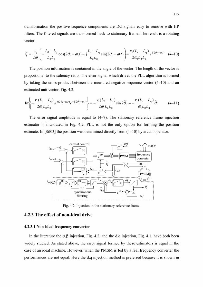
115
transformation the positive sequence components are DC signals easy to remove with HP
filters. The filtered signals are transformed back to stationary frame. The result is a rotating
vector.
)2(j
qdi
qdiir
qd
qdir
qd
qd
i
ii
ir2
)()2sin(j)2cos(
2ts e
LLLLv
tLLLL
tLLLLvi ωθ
ωωθωθ
ω−−
=⎟⎟⎠
⎞⎜⎜⎝
⎛−
−−−
−−= (4–10)
The position information is contained in the angle of the vector. The length of the vector is
proportional to the saliency ratio. The error signal which drives the PLL algorithm is formed
by taking the cross-product between the measured negative sequence vector (4–10) and an
estimated unit vector, Fig. 4.2.
θω
θωω
ωθωθ ~)(~2sin2
)(2
)(Im
qdi
qdir
qdi
qdi)ˆ2(j)2(
qdi
qdi irirLLLLv
LLLLv
eeLLLLv ttj −
−≈−
−=⎪⎭
⎪⎬⎫
⎪⎩
⎪⎨⎧ −− −−− (4–11)
The error signal amplitude is equal to (4–7). The stationary reference frame injection
estimator is illustrated in Fig. 4.2. PLL is not the only option for forming the position
estimate. In [Sil03] the position was determined directly from (4–10) by arctan operator.
iqe,ref
ide,ref = 0PI
e jθ PWM frequencyconverter
400 V
PMSMe-jθ
32
PI
+-
+-
id,q
PI
LP
εθ ωr
e jx ωit
2
HPe
jx
ωit
BP I
e jx
-ωit
θr
ii,n
i α,β
i α,β
current control
synchronous filtering
e-jx
θr
ii,n
+
+
Fig. 4.2 Injection in the stationary reference frame.
4.2.3 The effect of non-ideal drive
4.2.3.1 Non-ideal frequency converter
In the literature the α,β injection, Fig. 4.2, and the d,q injection, Fig. 4.1, have both been
widely studied. As stated above, the error signal formed by these estimators is equal in the
case of an ideal machine. However, when the PMSM is fed by a real frequency converter the
performances are not equal. Here the d,q injection method is preferred because it is shown in

Signal injection estimators 116
[Lin03a], [Lin03b] that the d,q injection is less sensitive to disturbances created by the
frequency converter.
The voltage distortion model of the frequency converters was discussed in Section 2.4.
This modelling is also valid for high frequency injection. Fig. 4.3 illustrates the behaviour of
the voltage and current vectors in the boundary between the current sectors I and II when the
α,β injection is applied. The current sector is changed when one of the phase currents crosses
zero. When the fundamental component of the current vector is is close to the sector boundary
the high frequency current component ii causes high frequency sector transitions. When the
sector is changed the error voltage caused by the converter also changes (2–44) , Fig. 4.3. The
maximum influence between both sectors can be expected when the fundamental current
angle is 30° + n⋅60°. The high frequency error voltage vector transitions distort the estimator
algorithm. Fig. 4.3 presents the distortion in the case of VSI. As discussed in Chapter 2, the
error voltage waveforms of IMC and DMC are more complicated. However, the strongest
voltage transitions occurs in the current sector boundary, also in the case of MC, Fig. 2.21 and
Fig. 2.22.
Fig. 4.4 illustrates the behaviour of the current and voltage vectors when the d,q injection
is performed. Now the current component with the injection frequency pulsates approximately
in the direction of the d-axis because ud,ref oscillates, Fig. 4.1. The sector transitions mainly
distort the d axis voltage. As presented in Section 4.2.1, the q axis current is used for speed
and position tracking. Therefore the voltage distortion is less harmful
0o
30
6090
o
oo
330o
180o
270o
is
iius
ui
I
IIIII
VIV
IVuerrI
uerrII
error voltagesof sectors I and II
30
6090
o
oo
isii
us
ui
I
IIIII
VIV
IV
Fig. 4.3 Voltage and current vector trajectories on the boundary between two sectors, α,β injection.
Fig. 4.4 Voltage and current vector trajectories on the boundary between
two sectors, d,q injection.
The effect of the frequency converter is also illustrated in Fig. 4.5 (α,β) and Fig. 4.6 (d,q).
The PMSM A (Appendix A) is driven in the Simulink model with direct speed and position

117
feedback. Thus rθ is replaced by θr in the estimator algorithms. Injection signals are
superimposed on the voltage reference signals as presented in Fig. 4.1 and Fig. 4.2. The
model of the non-ideal frequency converter is the same as in the simulations in Chapter 3. The
error signal εθ, which is the input for the PLL, is clearly more distorted in the case of α,β
injection, Fig. 4.5. Six sector transitions during the one fundamental period create the sixth
harmonic component to the torque and speed of the PMSM if the signal εθ is used to track the
rotor position. Therefore d,q injection is preferred.
Fig. 4.5 Error signal εθ, α,β injection. Nominal
load, 0.1 p.u. speed. Fig. 4.6 Error signal εθ, d,q injection. Nominal
load, 0.1 p.u. speed.
4.2.3.2 Higher order saliencies and current measurement errors
The estimator algorithms presented in the previous sections are based on the fundamental
frequency model, where Ld and Lq are constants. As presented in Chapter 2, the flux equations
contain multiples of the 6th harmonic of the fundamental motor supply frequency when they
are transformed to the rotor reference frame. Therefore the error signal (4–7), (4–11) contains
multiples of 6th harmonics and the same frequencies can be found in the torque produced by
the PMSM.
Errors of current measurement create effects similar to those presented in the simulations
in Section 3.6.2. Offsets create speed and torque oscillation at fundamental frequency
[Qia04]. Gain errors create 2nd harmonic. In general, an injection estimator is more sensitive
to current measurement errors than a model based estimator. Position error is tracked from the
signal with rather small amplitude compared to the fundamental frequency current. The
measured result may be distorted if A/D conversion is performed close to the time point when
the active vectors of the converter are changed. The distortion may be insiginicant for current
control and a model based estimator, but the relative error may be large when ii is concerned.
In this thesis A/D conversions are executed at the end of the modulation period. In the low
speed region, the end of tmod is reserved for a zero vector with relatively long duration because
the fundamental voltages are small. Thus the current oscillations should have decayed.
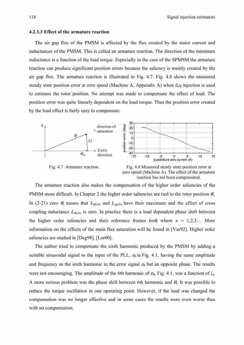
Signal injection estimators 118
4.2.3.3 Effect of the armature reaction
The air gap flux of the PMSM is affected by the flux created by the stator current and
inductances of the PMSM. This is called an armature reaction. The direction of the minimum
inductance is a function of the load torque. Especially in the case of the SPMSM the armature
reaction can produce significant position errors because the saliency is mainly created by the
air gap flux. The armature reaction is illustrated in Fig. 4.7. Fig. 4.8 shows the measured
steady state position error at zero speed (Machine A, Appendix A) when d,q injection is used
to estimate the rotor position. No attempt was made to compensate the effect of load. The
position error was quite linearly dependent on the load torque. Thus the position error created
by the load effect is fairly easy to compensate.
d axisdirection
q
Li
ψm
ψ
direction ofsaturation
Fig. 4.7 Armature reaction. Fig. 4.8 Measured steady state position error at zero speed (Machine A). The effect of the armature
reaction has not been compensated.
The armature reaction also makes the compensation of the higher order saliencies of the
PMSM more difficult. In Chapter 2 the higher order saliencies are tied to the rotor position θr.
In (2-21) zero θr means that Ldd,6n and Lqq,6n have their maximum and the effect of cross
coupling inductance Ldq,6n is zero. In practice there is a load dependent phase shift between
the higher order saliencies and their reference frames 6nθr where n = 1,2,3… More
information on the effects of the main flux saturation will be found in [Vas92]. Higher order
saliencies are studied in [Deg98], [Lor00].
The author tried to compensate the sixth harmonic produced by the PMSM by adding a
suitable sinusoidal signal to the input of the PLL, εθ in Fig. 4.1, having the same amplitude
and frequency as the sixth harmonic in the error signal εθ but an opposite phase. The results
were not encouraging. The amplitude of the 6th harmonic of εθ, Fig. 4.1, was a function of iq.
A more serious problem was the phase shift between 6th harmonic and θr. It was possible to
reduce the torque oscillation in one operating point. However, if the load was changed the
compensation was no longer effective and in some cases the results were even worse than
with no compensation.

119
4.2.4 Compensation of disturbances and other practical aspects
As discussed above, the frequency converter and additional saliencies of the PMSM create
multiples of the 6th harmonic in to the torque and speed of the PMSM. Compensation of the
dead time effect of the frequency converter is not crucial if d,q injection is applied. In the case
of α,β injection dead times must be taken into account [Sil02], [Sil03]. The effect of
additional saliencies of the PMSM still remains. In [Sil03] a so-called space modulation
profile is used to remove unwanted signals from the input of the PLL. The method is based on
the predefined tables. The commissioning of the tables is done off-line with data captured
during sensored operation. Measured position is used to form compensation signals which
remove harmonics from the input signals of the estimator. The initialization sequence is
performed with various load torques. The result is a two-dimensional look-up table giving
suitable compensation signals. In [Sil03] α,β injection is used, but a similar idea can be
applied in the case of d,q injection. The experimental results are quite promising. The
drawback of this method is the need for the sensor during the “teaching sequence”. Kalman
filter based heavy algorithms are also used to remove selected harmonics from a signal
[Car03]. In this thesis compensation methods are not studied in detail.
4.2.4.1 Initial angle detection
When the system is started the estimator finds the direction of the d-axis. However, there is
an uncertainty in the rotor position of 180 degrees since there are two inductance minima, one
in 0° direction and other in 180° direction. The simple method to check the direction of the
estimated d axis is to use a short drive sequence where the motor is fed by a constant q axis
current after the estimator has tracked the minimum inductance. The direction of rotation is
detected. If the estimated angle increases during the sequence with positive current the
estimator has found the correct d axis direction.
Rotating of the rotor is not always possible. A more sophisticated method is to exploit the
saturation of the stator iron. One method is to inject voltage pulses into both directions of the
estimated d axis. When the pulse causes a flux in the same direction as the PM flux the stator
iron becomes more saturated. This decreases the inductance. If the pulse causes opposite flux
the saturation decreases and the inductance increases. If the voltage pulses are strong enough
the inductance difference can be measured. A fairly comprehensive list of initial angle
detection methods based on the signal injection is given and a new method is developed in
[Kim04]. In this thesis initial angle detection methods are not studied.

Signal injection estimators 120
4.2.4.2 Selection of the frequency and the amplitude of the injection signal
The tuning of the high frequency injection estimator requires the selection of parameters
affecting the performance of the system. These parameters are: injection voltage (amplitude
and frequency), parameters of the selected signal processing method used to extract the useful
information from the measured currents and tuning of the PLL. Tuning of the PLL and filter
algorithms of the high frequency injection estimator will be described in Section 4.2.5.
The main principle is to select a injection frequency as high as possible. A higher
frequency means a faster estimator. The magnitude of the position error is known after half of
the injection signal period, Fig. 4.1. If ωi is high enough it does not affect the performance of
the current control because the injection components are outside the bandwidth of the control.
However, two factors restrict the maximum frequency. First, increased ωi decreases iiq which
decreases the accuracy of the system because the resolution of the current measurement is
limited. Very high ωi would require injection voltages which are not acceptable in practice.
Secondly, ωi is limited by the modulation frequency. If ωi is too high, one injection voltage
period is realised using only a few active voltage vectors. This increases the harmonics of the
iiqe and current measurements may be distorted due to the large voltage transients.
In this study one injection voltage period is composed of eleven voltage values. Therefore
the injection frequency is 909 Hz (1/(11*100 µs)). This frequency is clearly outside the
bandwidth of the current control. Frequencies 1 kHz, 1.111 kHz were also tested but the
performance of the estimator was impaired. Frequencies lower than 909 Hz did not improve
the results in the low speed region where injection methods were applied. In the literature,
[Jan03], [Sil03], [Wal04a], the injection frequency usually varies between 500 Hz and 1 kHz.
In [Cor98], [Lin02] the injection frequency was 2 kHz.
In matrix converter drives (Machine A) the amplitude of ui was 40 V. In VSI drive
(Machine B) the amplitude was 80 V. In the matrix converter drive the amplitude of the iid
was approximately 1.1 A (10% of the nominal). In the VSI drive the amplitude was 3 A. The
resolution of the current measurement of the MC drive was 50 mA and 250 mA in the case of
the VSI drive with Machine B.
The amplitudes of the injection currents are higher than would be expected on the basis of
the inductance values of Appendix A. Inductances are smaller for the higher frequencies
because it is more difficult for high frequency flux components to penetrate the iron parts of
the rotor and the permanent magnets. Thus leakage inductances become more dominant when
frequency is increased.

121
4.2.5 Tuning of the signal injection estimator
The high frequency injection estimator, Fig. 4.1, includes signal processing algorithms not
needed in the basic PLL applied in the model based estimators. In this thesis, Fig. 4.1, the
injection frequency component is separated from the measured iqe by a second order band-
pass (BP) filter. The filter type is Butterworth. When the PLL is analysed the amplitude of the
iiqe (4–7) is replaced by a DC signal. The PB filter is then replaced by a first order LP filter
which gives the envelope of the BP filter, Fig. 4.10. The block diagram of the PLL in the
frequency domain is illustrated in Fig. 4.9. Now the PLL is a third order system. The LP filter
used for the smoothing of the demodulated signal, Fig. 4.1, is not concerned because its time
constant may be one tenth of τ in Fig. 4.9. The step responses of the BP filter used in this
thesis and the “equivalent” LP filter are shown in Fig. 4.10. The magnitude response and the
discrete transfer function of the BP filter are shown in Fig. 4.11. The time constant τ is
2.2 ms. The application specific gain Kinj was introduced in (4–7).
LP
I
ε ωr
θr
Ik1
k2 +
K+θr -
Kk1
1τs+1
θr1/s
1/sI
1/s
ωrτs3+s2+Kk1s+Kk2
ωr(s)=ωr(s)
Fig. 4.9 Relation between ωr and estimated speed in the PLL used for speed and position estimation.
Fig. 4.10 Step response of the BP filter and “equivalent” LP filter. Input signals are dashed.
Fig. 4.11 Amplitude response and the transfer function of the BP filter.
Filtering naturally narrows the bandwidth of the PLL. Thus the filter should be as fast as
possible. A fast filter means that the amplitude of the filter output iiqe rapidly follows the
changes of the position error. The drawback is the lesser damping of the frequencies around
ωi. In fast current transients other frequencies pass the filter and disturb the estimation
process. Heavy damping around the injection frequency gives a “clean” signal but the
performance of the speed control is impaired.
The BP filter is not the only algorithm used to extract iiqe from iqe. In [Wal04a] high-pass

Signal injection estimators 122
filters with very low bandwidths were used to remove the DC-level of the measured current.
These filters are sensitive to disturbances and serious problems may occur during transients,
especially in servo drives, where mechanical time constants are small. In [Lep03], [Pii04] the
DC-level is removed by using moving average (MA) and trend removing alogorithms.
[Lep03] concentrated on low frequency injection but the idea of the estimator is similar to
high frequency methods. In a MA filter n samples of data are stored and the sum of samples is
divided by n. In every calculation period the oldest sample is replaced by the newest. The
filter can remove frequency multiples of 1/(nts), where ts is the sample time.
In this thesis a BP filter is preferred because it has better properties in fast current
transients. In Fig. 4.12 a signal with a frequency of 1 kHz is extracted from the input signal by
a BP filter and the MA algorithm where the MA of 1 ms (n = 10) is subtracted from the input
signal. In steady state both algorithms give similar results. If the DC level of the input signal
is rapidly changed the output of the MA algorithm is more heavily distorted. The MA filter
removes only certain frequencies as explained above. On the other hand the MA filter is faster
and does not contain the LP filter type delay presented in Fig. 4.10, when the magnitude of
the position error changes rapidly. Because a MA algorithm filters effectively only the
multiples of 1/(nts) the signal may require stronger LP filtering after the demodulator
compared to the case when a BP filter is used, Fig. 4.1
Fig. 4.12 Comparison of responses of the band-pass filter (BP) and the moving average filter (MA).
The estimated speed (output of the PLL) must be filtered to prevent the amplification of
distubances in the speed control loop. Here a second order Butterworth type LP filter was
used. The filter has a double pole in –400/s. Let us assume that a second order LP filter is
tuned to attenuate a certain frequency by the same amount as a first order filter. The step
response of the higher order filter is clearly faster. The bandwidth of the speed control loop is
therefore increased. In this thesis a second order LP filter was used to filter the speed estimate
in the simulations and measurements.
The benefits of second order filters are clear in the case of machine A, which is a small
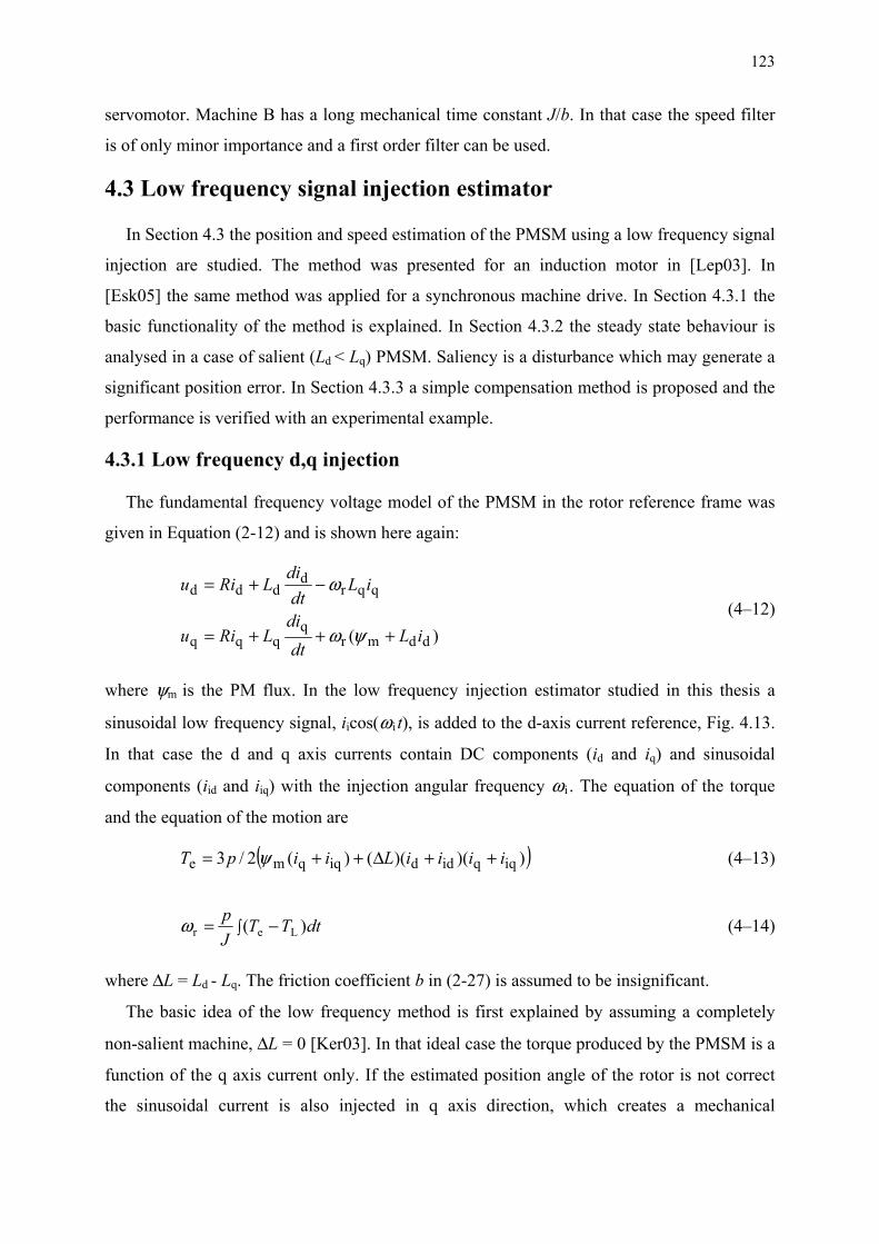
123
servomotor. Machine B has a long mechanical time constant J/b. In that case the speed filter
is of only minor importance and a first order filter can be used.
4.3 Low frequency signal injection estimator
In Section 4.3 the position and speed estimation of the PMSM using a low frequency signal
injection are studied. The method was presented for an induction motor in [Lep03]. In
[Esk05] the same method was applied for a synchronous machine drive. In Section 4.3.1 the
basic functionality of the method is explained. In Section 4.3.2 the steady state behaviour is
analysed in a case of salient (Ld < Lq) PMSM. Saliency is a disturbance which may generate a
significant position error. In Section 4.3.3 a simple compensation method is proposed and the
performance is verified with an experimental example.
4.3.1 Low frequency d,q injection
The fundamental frequency voltage model of the PMSM in the rotor reference frame was
given in Equation (2-12) and is shown here again:
)( ddmr
qqqq
qqrd
ddd
iLdt
diLRiu
iLdt
diLRiu
+++=
−+=
ψω
ω (4–12)
where ψm is the PM flux. In the low frequency injection estimator studied in this thesis a
sinusoidal low frequency signal, iicos(ω i t), is added to the d-axis current reference, Fig. 4.13.
In that case the d and q axis currents contain DC components (id and iq) and sinusoidal
components (iid and iiq) with the injection angular frequency ω i . The equation of the torque
and the equation of the motion are
( )))()(()(2/3 iqqiddiqqme iiiiLiipT ++∆++= ψ (4–13)
dtTTJp )( Ler −= ∫ω (4–14)
where ∆L = Ld - Lq. The friction coefficient b in (2-27) is assumed to be insignificant.
The basic idea of the low frequency method is first explained by assuming a completely
non-salient machine, ∆L = 0 [Ker03]. In that ideal case the torque produced by the PMSM is a
function of the q axis current only. If the estimated position angle of the rotor is not correct
the sinusoidal current is also injected in q axis direction, which creates a mechanical

Signal injection estimators 124
oscillation. The actual q axis current oscillating with frequency ω i can be written
rii
~jiiiq
~sin)cos(e0)cos(Im r
refide,
θωω θ tijtiii
−≈⎪⎭
⎪⎬
⎫
⎪⎩
⎪⎨
⎧
⎟⎟⎟
⎠
⎞
⎜⎜⎜
⎝
⎛+≈ −
43421 (4–15)
The equation of iiq is an approximation, because the actual currents do not follow their
references perfectly. (4–15) is substituted into the equation of torque (4–13). The oscillating
torque is substituted into (4–14). The load torque TLoad is assumed to be constant, and it can
thus be omitted because it does not contain any components with injection frequency. Now it
is possible to write an expression for the back-emf oscillating with the injection frequency ω i .
ri
i2m
2iir
i2m
2mriq
~sin2
3)sin()cos(~sin
23 θ
ωψωωθψψωJ
iptdtt
Jip
e =∫=−= (4–16)
Finally the actual oscillating q axis back-emf (4–16) is transformed into the estimated d,q
frame with angle rθ . The oscillating back-emf component in the reference frame of the
control system is
ri
i2m
2
iri
i2m
2
ir
~jiqiqe
~2
3)sin(~sin2
3)sin(~cosejIm r θω
ψωθω
ψωθθ
Jipt
Jiptee ≈== (4–17)
(4–17) is a suitable error signal for a PLL type algorithm. Equation (4–17) has a similar form
to the error equation of the high frequency estimator, (4–7). The amplitude of the oscillating
back-emf eiqe is proportional to the square of the number of pole pairs and inversely
proportional to the inertia J.
Estimator structure
The estimate of the oscillating back-emf in the q direction (4–17) is obtained using the
basic voltage equation in the estimated rotor reference frame (4–12).
dedrqe
qqeqeqemdedrqe
qqeqeˆˆˆˆ)( iL
dtdi
LiRueiLdt
diLRiu ωψω +++−=⇒+++= (4–18)
A BP filter is used to extract eiqe from the estimated back-emf eqe (4–18). In [Lep03] the
filtering is achieved by removing the trend and average from eqe. The position error is
demodulated by multiplying the extracted signal by sin(ω i t), Fig. 4.13.

125
I LP
BP
θr
iqe,ref
ide,refPI
+
++
e jθud,ref
uq,refPWM frequency
converter
400 V
PMSMe-jθ
32
PI
+ -
+ -
ide
iqe
iαiβ
ed
PIεθ
iicos(ωit)
uq
ire -uq + Riqe + L + Lideωrdtdiqe
eqe
sinωit
θ
ωr
ω2
+ω1
eiqe
Estimator
Current control
ω2= (uq,ref - Riqe )/ψm
eq
+
Fig. 4.13 Basic structure of the current control and low frequency estimator.
If the motor is symmetric and the rotor speed is close to zero the PLL algorithm drives the
position error to zero in steady state operation. In practice there is always some saliency even
in the case of surface magnet motors. The effect of saliency and interaction between speed
and oscillating current components may cause severe errors in the estimated position if they
are not properly compensated.
The dynamic performance of the low frequency signal injection is rather poor because the
position error information is extracted from a low frequency signal. The injection frequency
ω i varies between a few Hz and a few hundred Hz depending on p2/J ratio (4–17). The
dynamic performance of the estimator can be improved by also exploiting the speed
information of the average component of eq e [Lep03]. In Fig. 4.13 the output of the direct
speed estimator is denoted as 2ω .
4.3.2 Analysis of the steady state behaviour
If the PMSM is loaded and there is an error between the actual and the estimated position
the current seen by the control system is
rqrdeqrqrdderr
~jre ~cos~sin,~sin~cos θθθθθ iiiiiiiei +=−=⇔= (4–19)
The current control drives the average of ide to zero. Thus in steady state
rqd~tanθii = . (4–20)
iq is dependent on the load and on the position error. If the position error is within an
acceptable range: iq ≈ 2TLoad/3pψm. The BP filter, Fig. 4.13, removes from eqe (4–18) all but
the frequencies ω i . Therefore the DC component (idiq) and the component with frequency 2ω i
(iidiiq) are omitted from the equation of the torque (4–13). Using (4–13) and (4–14) the speed

Signal injection estimators 126
in steady state is
( ) tdiiiiLiJpdtT
Jp
444444 3444444 21ir
)(2
3idqiqdiqm
2r0ier0irr0r
ω
ψωωωωω ∫ +∆++=∫+=+= , (4–21)
where ω r0 is the average speed and ω i r is the oscillating speed with frequency ω i . Now we
can write the voltage equation (4–12) in the actual synchronous reference frame. Only the
components with frequency ω i are included.
irmdiridr0diq
qiqiq
qiriqr0qid
didid
)(
)(
ωψωω
ωω
++++=
+−+=
iiLdt
diLRiu
iiLdt
diLRiu
(4–22)
Using (4–19) - (4–22) we can built a model in a more convenient form for the steady state
analysis of the low frequency estimator, Fig. 4.14. This model contains the current control,
PMSM and the block calculating the oscillating back-emf eiqe. The “e” block of Fig. 4.14 is
simplified by omitting the derivative of iq. This can be done because the steady state
performance is analysed and the iq reference contains no component with frequency ω i . For
the same reason the speed control is excluded.
Lds+R1
-+
+ +
Lqs+R1
PI
e-jθr e jθr
iideiid
PI
uide
iide
0
iide,ref
eiqe-uiqe+Ldiide,refωr0
+
-
-
+
uid
uiq
ω r0PMSM
Lq(ωiriq +ωr0iiq)
Ld(ωirid +ωr0iid)+ψmωiruiqe
iiq iiqe
iiqe iide,ref
uiqee
Fig. 4.14 Simplified structure of the control system and low frequency estimator.
Using Fig. 4.14 it is possible to write a transfer function between the back-emf eiqe and iide
reference [Esk05].
r0d23qdp
4qd
r2
qr2
dr02r2
ip
refide,
iqee ˆ
)))(((
)~sin~cos(2
)~2sin()(
)(
)()( ω
θθωθ
LsDCsBssLLRKsLL
AsLLsL
KsK
si
sesG +
++++++
⎟⎟⎠
⎞⎜⎜⎝
⎛+++
∆+−
==
(4–23)

127
where
)(2
3
)
)((23
)(2
32)(
)(2
3)()(
)~cos)(~sin(2
3))((4
)~2sin(3
dmqqddi
22i
qmd
ddqqqd2
r0ddqqdm
2ip
qqqdddddm2
qdi2
pqd2r0
r2
qddmr2
q2
dmddqqr
2
ψψψψ
ψψ
ψψω
ψψψψ
ψψψψω
θψψθψψψψψθ
+∆−∆+=
++∆+⎟⎟
⎠
⎞
⎜⎜
⎝
⎛∆+∆−++=
⎟⎟
⎠
⎞
⎜⎜
⎝
⎛∆−∆++++++=
∆+∆++++∆−=
iLiLJKp
KD
L
iLiLLJp
iLiLJ
pKRKC
iLLiLLLJ
pLLKRKLLB
iLLiJ
piiLJ
pA
In (4–23) Kp is the gain of the PI controller and Ki is the gain Kp divided by the integration
time ti. ψd and ψq are flux linkage components (ψm + Ldid) and Lqiq. If the rotor speed is near
zero and the PI controller gains (Ki, Kp) are large the denominator of (4–23) approaches s(Kps
+ Ki)2. If this approximation is used we can write a simplified expression for the gain and
phase of (4–23). The simplified model does not take the tuning of the PI controllers into
account.
( )
( )
⎟⎟⎟⎟⎟⎟
⎠
⎞
⎜⎜⎜⎜⎜⎜
⎝
⎛
+−
⎟⎟⎠
⎞⎜⎜⎝
⎛+
∆−
≈
⎟⎟⎠
⎞⎜⎜⎝
⎛+
∆−++≈
−
)~sin~cos(
2)~2sin(
tan)(Phase
2)~2sin(
)~sin~cos()(Gain
r2
qr2
dr0
ii
r
1e
2
ii
r2r
2qr
2d
2r0e
θθω
ωωθ
ωωθθθω
LL
AL
sG
ALLLsG
(4–24)
The effect of saliency at zero speed
First the position error r~θ is assumed to be zero. The only nonzero component in the gain
is 3p2∆Lψdiq/2J inside the coefficient A, (4–24). The phase shift is approximately -π/2. This
can be concluded from (4–24) because the denominator of the lower expression is very small
(the speed ωr0 is near zero). In the demodulation process, Fig. 4.13, eiqe is multiplied by a
signal with -π/2 phase lag compared to iide,ref = iicos(ωit). Thus the eiqe has a non-zero
amplitude and is in phase with the demodulation signal. The error signal εθ is larger than 0.
The estimated position increases. The next important operating point is the position error
where the torque oscillation with the angular frequency ω i is zero. This is the case when the
coefficient A is zero. However, the position estimate still increases because the saliency
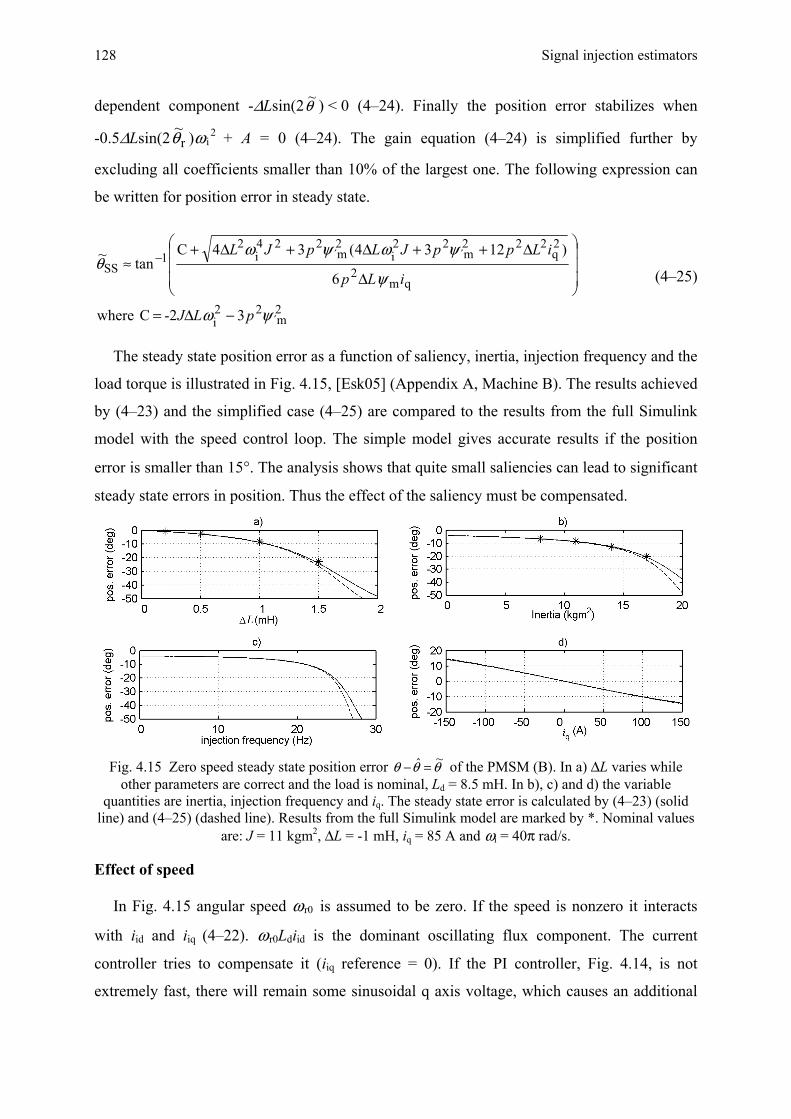
Signal injection estimators 128
dependent component -∆Lsin(2θ~ ) < 0 (4–24). Finally the position error stabilizes when
-0.5∆Lsin(2 r~θ )ω i
2 + A = 0 (4–24). The gain equation (4–24) is simplified further by
excluding all coefficients smaller than 10% of the largest one. The following expression can
be written for position error in steady state.
2m´
22i
qm2
2q
222m´
22i
2m´
224i
21
SS
3-2Cwhere
6
)1234(34Ctan~
ψω
ψ
ψωψωθ
pLJ
iLp
iLppJLpJL
−∆=
⎟⎟⎟
⎠
⎞
⎜⎜⎜
⎝
⎛
∆
∆++∆+∆+≈ −
(4–25)
The steady state position error as a function of saliency, inertia, injection frequency and the
load torque is illustrated in Fig. 4.15, [Esk05] (Appendix A, Machine B). The results achieved
by (4–23) and the simplified case (4–25) are compared to the results from the full Simulink
model with the speed control loop. The simple model gives accurate results if the position
error is smaller than 15°. The analysis shows that quite small saliencies can lead to significant
steady state errors in position. Thus the effect of the saliency must be compensated.
Fig. 4.15 Zero speed steady state position error θθθ ~ˆ =− of the PMSM (B). In a) ∆L varies while
other parameters are correct and the load is nominal, Ld = 8.5 mH. In b), c) and d) the variable quantities are inertia, injection frequency and iq. The steady state error is calculated by (4–23) (solid
line) and (4–25) (dashed line). Results from the full Simulink model are marked by *. Nominal values are: J = 11 kgm2, ∆L = -1 mH, iq = 85 A and ωi = 40π rad/s.
Effect of speed
In Fig. 4.15 angular speed ω r0 is assumed to be zero. If the speed is nonzero it interacts
with iid and iiq (4–22). ω r0Ldiid is the dominant oscillating flux component. The current
controller tries to compensate it (iiq reference = 0). If the PI controller, Fig. 4.14, is not
extremely fast, there will remain some sinusoidal q axis voltage, which causes an additional

129
error to eiqe. It can be seen in (4–24) that non-zero ω r0 changes the amplitude and the phase
shift of eiqe. The steady state error is now clearly dependent on the tuning of the current
control. Thus the simple model (4–24) gives accurate results only if the angular frequency ω r0
is zero or very low. Fig. 4.16 shows the error when the speed varies between -10% and 10%
speed. The results are calculated with three ti using (4–23). If ti is kept constant and Kp varies
the results are very similar. Increased inertia and saliency increase the speed dependent error.
However, this speed error also exists when Ld = Lq.
Fig. 4.16 Steady state position error as a function
of speed. Load and the other parameters are nominal.
4.3.3 Compensation of the steady state position error
A major steady state error in the position estimate can be prevented by injecting a
convenient low frequency signal in the q axis direction. The idea is to cancel the reluctance
component from the equation of the torque. Let us assume that iiqe,ref ≠ 0. Now iid and iiq are:
(iid + jiiq) ≈ (iide,ref + jiiqe,ref) r~θje− . iid and iiq are are substituted into the equation of the torque
(4–13). There is no torque oscillation with frequency ω i if the position error is zero and
dm
qrefide,refiqe, Li
Liii
∆+
∆−=
ψ (4–26)
The reference signal in the q direction is in phase with the main injection signal iide,ref.
Even if the position error is not zero the injection of (4–26) compensates the effect of the
reluctance torque with good accuracy. In practice the non-ideal current controllers cause a
small error. The saliency ratio, inertia and other parameters restrict the use of this
compensation method. Even if injecting (4–26) removes the other coefficients with ∆L from
the numerator of (4–23) there remains a component 0.5∆Lsin(2 r~θ ). If it increases faster than
the coefficient A (4–23) when the position error increases the system is unstable or at least the
steady state error becomes considerable. If the slopes of these two coefficients are studied
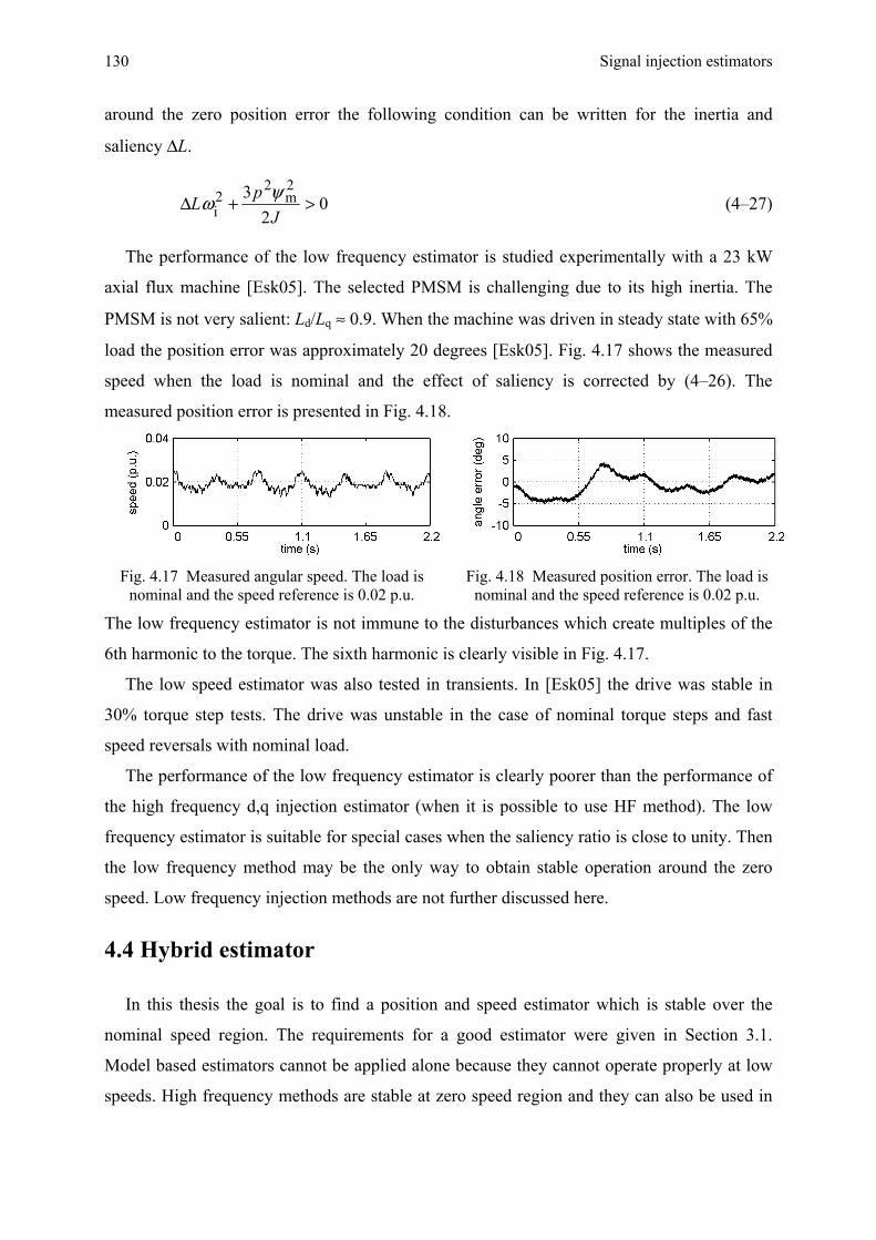
Signal injection estimators 130
around the zero position error the following condition can be written for the inertia and
saliency ∆L.
02
3 2m
22i >+∆
JpL ψω (4–27)
The performance of the low frequency estimator is studied experimentally with a 23 kW
axial flux machine [Esk05]. The selected PMSM is challenging due to its high inertia. The
PMSM is not very salient: Ld/Lq ≈ 0.9. When the machine was driven in steady state with 65%
load the position error was approximately 20 degrees [Esk05]. Fig. 4.17 shows the measured
speed when the load is nominal and the effect of saliency is corrected by (4–26). The
measured position error is presented in Fig. 4.18.
Fig. 4.17 Measured angular speed. The load is nominal and the speed reference is 0.02 p.u.
Fig. 4.18 Measured position error. The load is nominal and the speed reference is 0.02 p.u.
The low frequency estimator is not immune to the disturbances which create multiples of the
6th harmonic to the torque. The sixth harmonic is clearly visible in Fig. 4.17.
The low speed estimator was also tested in transients. In [Esk05] the drive was stable in
30% torque step tests. The drive was unstable in the case of nominal torque steps and fast
speed reversals with nominal load.
The performance of the low frequency estimator is clearly poorer than the performance of
the high frequency d,q injection estimator (when it is possible to use HF method). The low
frequency estimator is suitable for special cases when the saliency ratio is close to unity. Then
the low frequency method may be the only way to obtain stable operation around the zero
speed. Low frequency injection methods are not further discussed here.
4.4 Hybrid estimator
In this thesis the goal is to find a position and speed estimator which is stable over the
nominal speed region. The requirements for a good estimator were given in Section 3.1.
Model based estimators cannot be applied alone because they cannot operate properly at low
speeds. High frequency methods are stable at zero speed region and they can also be used in

131
the nominal speed region [Lin03b]. However, at higher speeds model based methods have
attractive features, hence the motivation for a hybrid estimator.
The main drawbacks of high frequency injection estimators are:
- Need for injection voltage. Injection creates additional acoustic noise and power losses,
- Modulation index greater than unity may be demanded by the control if the machine is
operating with nominal speed and an injection voltage with high amplitude is added to the
voltage references,
- Higher demands for the performance of the current measurement system.
In Chapters 3 and 4 several model based estimators and injection estimators were
discussed. The model based estimator presented in Section 3.4.5 is used at higher speeds. In
the low speed region d, q injection is applied.
An important issue is the change of the method. It cannot be done suddenly because it
would cause unwanted oscillation if the drive operates near the border speed. In [Wal04a] the
transition between the model based and the injection estimator is made by linear transition
functions, Fig. 4.19. This method is also used here.
The position error signal is calculated by the voltage model, Fig. 3.12, and the injection
method, Fig. 4.1. Both error signals are multiplied by their transition function and added
together. If |ωr| > ωh the estimator is completely model based. If |ωr| < ωl, the position error is
corrected using only the signal injection method. When |ωr| >ωh the amplitude of the injection
signal vi is decreased linearly toward zero as a function of |ωr|.
ωr
0
1
weighting coefficient
injection model basedmodel based
-ωrωl ωh-ωl-ωh
Fig. 4.19 Transition function providing smooth transition between estimation methods.
Fig. 4.20 shows the hybrid estimator used in this study. The estimator is the same as that
presented in Fig. 3.12 (combined Matsui estimator). The only addition is the “filtering and
demodulation” block from Fig. 4.1. The direct speed estimator (lower branch in Fig. 4.20 with
output 2ω ) is always active. It was found that the performance of the estimator is improved at
low speeds if the signal injection estimator is assisted by the simple model based speed
estimator.

Signal injection estimators 132
εθ,modωr
θr(k+1)tsk1
k2
+-ud,ref+Ride-ωrLqiqeωr(k)ude,ref +
k+
+ −
iqe(k+1)
iqe(k+1)+
ω2(k+1)
delay (ts)
(uqe-Riqe-ω2(Ldide+ψm))(ts/Lq)
+ts
+
ω1(k+1)
ω2(k+1)
uqe,refire
ω2(k)
to speed control
iqe(k)
+
transition
εθ,injiqe
filtering and demodulation
BP LPsin(ωit) pre-gain
ωr
Fig. 4.20 Discrete time implementation of the hybrid estimator.
In [Pii05] the injection estimator does not directly take part in calculating the speed
estimate. The injection branch has its own PI controller and the output of the PI algorithm is
used to correct the speed estimate which adjusts the adaptive model. When |ωr| increases the
effect of injection is reduced by linearly decreasing the amplitude of vi and gains of the PI
controller.
4.5 Simulations of injection and hybrid estimators
The modelling of the d,q injection estimator and the hybrid estimator is performed in the
Matlab Simulink environment. The tuning of the speed controller, current controllers and
estimator algorithms are presented in Table 4.1. The motor parameters are from Appendix A
(Machine A).
Simulations are carried out with d,q injection estimator alone Fig. 4.1 and with the hybrid
estimator Fig. 4.20. When d,q injection is not assisted by the model based algorithm the gains
of the PLL are constants because the application specific gain K (3-12) is not speed
dependent. Poles are placed at the real axis as explained in Section 3.3.
In the hybrid estimator the model based estimator is the combined Matsui method
presented in Section 3.4.5. As discussed in Section 3.4.3, the gains of the PLL vary as a
function of speed ωr when a back-emf estimator is applied (3-38). When ωr < ωlow the gains k1
and k2 are constants, Table 4.1. The gain ( Kinj = vi(Ld-Lq)/ωiLdLq ) of the injection estimator
(4–7) is clearly smaller than the gain ωrψm (3-35) of the model based estimator when ωr <
ωlow = ωh. Gains of the PLL are constants when the estimated ωr is below ωlow (3–38).
Therefore the output of the injection branch, Fig. 4.20, is multiplied by a “pre-gain”
(ωlowψm)/Kinj This ensures that the error signals εθ,inj and εθ,mod are approximately equal when
the injection branch is active. In the case of motor A (Appendix A), pre-gain is approximately

133
70. The border frequencies ωl and ωh of the hybrid estimator are 0.09 p.u and 0.18 p.u.
respectively, Fig. 4.19. The 2nd order LP filter in speed feedback has a double pole in -400/s.
Table 4.1 Parameters of the control system and estimators.
kp ti PLL of the estimator ω l o w k
Speed control 1.8 0.03 s Current control 20 0.005 s
Model based in hybrid k1 = ρ2/K, k2 = 2ρ/K (ρ = 80/s and K =ω rψm)
0.18 p.u. 120
d,q injection in hybrid same as above (K always (0.18*471)ψm) d,q injection alone k1 = 7002, k2 = 2*700
4.5.1 Low speed simulations
First the pure injection estimator and hybrid estimator are compared. The speed is changed
from zero to 0.05 p.u. and then the sign of the speed reference is changed. After the machine
has been decelerated to zero speed the sign of the nominal load torque is changed from 100%
to -100% value at 0.75 s. Fig. 4.21 and Fig. 4.22 show the simulated speed and position error.
Fig. 4.23 and Fig. 4.24 illustrate the same sequence in the case of the hybrid estimator.
Because the speed estimate is under 0.09 p.u. the signal εd,mod is not used to correct the
estimated position. However, the direct speed estimator of the hybrid estimator with output
2ω is active, Fig. 4.20.
The overshoot of the simulated speed is significant. The reason is not the tuning of the
speed controller. The current transient disturbs the injection estimator. For a short period after
the transient the estimated speed increases into a wrong direction.
The performance of the hybrid estimator is better even if the slower PLL tuning is used
compared to the pure d,q injection version, Table 4.1. This is an advantage because the
estimator is less sensitive to disturbances if the gains of the PLL can be decreased.
Fig. 4.21 d,q injection, speed reference and simulated speed, nominal load.
Fig. 4.22 d,q injection, position error ( rr θθ − ), nominal load.
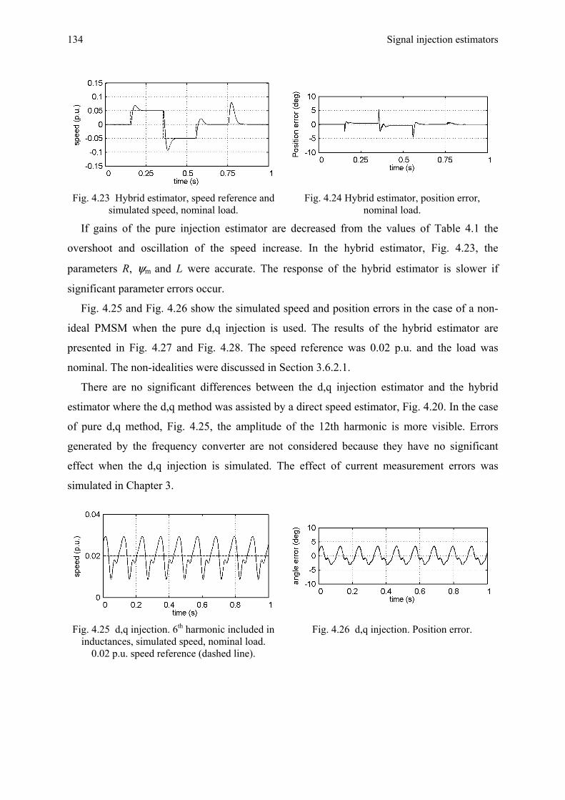
Signal injection estimators 134
Fig. 4.23 Hybrid estimator, speed reference and simulated speed, nominal load.
Fig. 4.24 Hybrid estimator, position error, nominal load.
If gains of the pure injection estimator are decreased from the values of Table 4.1 the
overshoot and oscillation of the speed increase. In the hybrid estimator, Fig. 4.23, the
parameters R, ψm and L were accurate. The response of the hybrid estimator is slower if
significant parameter errors occur.
Fig. 4.25 and Fig. 4.26 show the simulated speed and position errors in the case of a non-
ideal PMSM when the pure d,q injection is used. The results of the hybrid estimator are
presented in Fig. 4.27 and Fig. 4.28. The speed reference was 0.02 p.u. and the load was
nominal. The non-idealities were discussed in Section 3.6.2.1.
There are no significant differences between the d,q injection estimator and the hybrid
estimator where the d,q method was assisted by a direct speed estimator, Fig. 4.20. In the case
of pure d,q method, Fig. 4.25, the amplitude of the 12th harmonic is more visible. Errors
generated by the frequency converter are not considered because they have no significant
effect when the d,q injection is simulated. The effect of current measurement errors was
simulated in Chapter 3.
Fig. 4.25 d,q injection. 6th harmonic included in inductances, simulated speed, nominal load.
0.02 p.u. speed reference (dashed line).
Fig. 4.26 d,q injection. Position error.
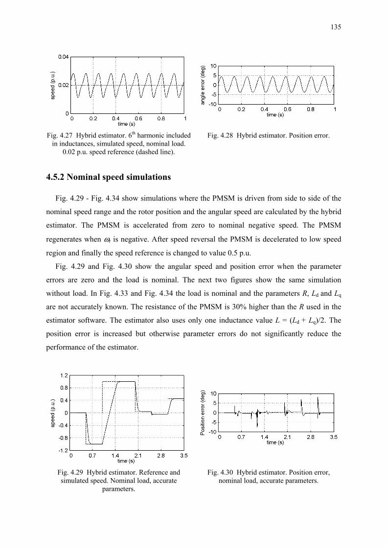
135
Fig. 4.27 Hybrid estimator. 6th harmonic included in inductances, simulated speed, nominal load.
0.02 p.u. speed reference (dashed line).
Fig. 4.28 Hybrid estimator. Position error.
4.5.2 Nominal speed simulations
Fig. 4.29 - Fig. 4.34 show simulations where the PMSM is driven from side to side of the
nominal speed range and the rotor position and the angular speed are calculated by the hybrid
estimator. The PMSM is accelerated from zero to nominal negative speed. The PMSM
regenerates when ωr is negative. After speed reversal the PMSM is decelerated to low speed
region and finally the speed reference is changed to value 0.5 p.u.
Fig. 4.29 and Fig. 4.30 show the angular speed and position error when the parameter
errors are zero and the load is nominal. The next two figures show the same simulation
without load. In Fig. 4.33 and Fig. 4.34 the load is nominal and the parameters R, Ld and Lq
are not accurately known. The resistance of the PMSM is 30% higher than the R used in the
estimator software. The estimator also uses only one inductance value L = (Ld + Lq)/2. The
position error is increased but otherwise parameter errors do not significantly reduce the
performance of the estimator.
Fig. 4.29 Hybrid estimator. Reference and simulated speed. Nominal load, accurate
parameters.
Fig. 4.30 Hybrid estimator. Position error, nominal load, accurate parameters.

Signal injection estimators 136
Fig. 4.31 Hybrid estimator. Reference and simulated speed. No load, accurate parameters.
Fig. 4.32 Hybrid estimator. Position error, no load, accurate parameters.
Fig. 4.33 Hybrid estimator. Simulated speed. Nominal load, RR ˆ− = 0.3 Ω (30%). L = 0.01 H.
Fig. 4.34 Hybrid estimator, position error, nominal load. RR ˆ− = 0.3 Ω (30%). L = 0.01 H.
In the step response tests above the estimated ωr rapidly crosses the speed range between ω l
and ωh, Fig. 4.19. In the next two figures the load torque is nominal and the speed is reversed
by using a rather slow ramp reference signal. The parameter errors are same as above, Fig.
4.33. The position error, Fig. 4.36, contains a small steady state error but otherwise the
behaviour of the system is good. The steady state error is created by parameter errors. In that
case the incorrent q axis inductance estimate produces a position error (3-41).
Fig. 4.35 Hybrid estimator. Simulated speed. Nominal load, RR ˆ− = 0.3 Ω, L = 0.01 H.
Fig. 4.36 Hybrid estimator, position error. Nominal load, RR ˆ− = 0.3 Ω, L = 0.01 H.

5. Realisation of the experimental setup
5.1 Experimental VSI drive
Fig. 5.1 illustrates a schematic diagram of the VSI drive used in this thesis. A 23 kW axial
flux PMSM (machine B in Appendix A) is fed by a voltage source frequency converter,
Appendix B. The rectifier is a three-phase diode bridge. In the DC link two 3300 µF 350 V
electrolytic capacitors are connected in series. The rated power of the frequency converter is
50 kW. The load machine is a 50 kW separately excited DC machine fed by a thyristor
rectifier (ABB, DCS500). The power transmission between the PMSM and the DC-machine
is implemented with a cogged belt. A photograph of the setup will be found in Appendix A.
a
c
b
i iA BuDC-
uDC+ DC-machine
+-
DCS500
Ia
a
c
b
Tacho
Resolver
R/DScaling
gatedriver
0...100 V
PC
A/D
MPC555ω (0...5 V)
i iA BuDC-uDC+
GAL
Userinterface
User interface
MPC555 board
θ(12 )bit
Originalcontrol board
VSIPMSM (MX18)
400 V
400 V
IO
Fig. 5.1 Schematic diagram of the VSI drive.
The original control board of the frequency converter is replaced by an MPC555 control
board, designed at the Institute of Power Electronics (TUT). The heart of the control board is
the MPC555 microcontroller. The board also contains the auxiliary circuits needed by the
peripherals of MPC555 and the GAL circuits (generic array logic) needed for modulation and
protection purposes. The GAL circuits create switching signals (0…5 V) for each inverter leg.
A positive signal means that the upper IGBT is conducting. Dead time generation is done by
an IXYS IXDP631 circuit in the original gate driver board. The user interface is a PC with
Matlab. The PC and MPC555 communicate via RS-232 serial interface. DCS500 has its own
control panel.

Realisation of the experimental setup 138
Measurements
The quantities measured are two load currents for the control system and the estimator, the
DC link voltage for the modulator, the rotor angular speed and the rotor position angle for
analytical purposes. Current measurements of phases A and B are made with Hall-effect
based LEM LA100-P current transducers. The current signal is converted into 0…5 V voltage
signal where -130 A, 0 A, and 130 A correspond 0 V, 2.5 V and 5 V respectively. The voltage
signal is the input of the 10 bit A/D converters of MPC555, Fig. 5.1. Thus the resulting
current resolution is approximately 250 mA. The DC link voltage is scaled by a resistance
circuit into level 0…5 V where 750 V corresponds to 5 V.
The angular speed is measured with a tachometer (Radio-Energie, RE.0444 L1B) and the
voltage is scaled to 0…5 V level with the circuits of the original control board before being
transformed to the digital form in the MPC555. The rotor position is measured with a resolver
(Smartsyn). The analogue sine and cosine signals are converted to a digital form by the
resolver to digital (R/D) converter (Analog Devices, AD2S81A). The resolution of the
position measurement is 12 bit. The R/D converter and MPC555 communicate via general
purpose I/O pins of MPC555. The measured speed and position are used as references when
the performance of the sensorless operation is verified.
Protection
The experimental setup of Fig. 5.1 contains two overcurrent and overvoltage protection
systems. The control software disables the VSI (all switches are opened) if too high current or
voltage is detected. The MPC555 board also includes a hardware protection which disables
the VSI bridge when any of the input voltages of the A/D converters exceeds a predetermined
level. The fault signal is routed to the MPC555 and also to the logic circuitry (GAL). Thus the
VSI can be disabled even if the software operation fails.
5.2 Experimental matrix converter drive
The structure of the matrix converter setup is described in Fig. 5.2, where the MC can be
the indirect or the direct topology. The matrix converter feeds the 3.5 kW radial flux PMSM,
Appendix A. The load is a 6.3 kW separately excited DC machine fed by a thyristor rectifier
(Siemens, Simoreg K 6RA24). The rated power of the MC prototypes is 5 kVA. Photographs
of the setup will be found in Appendix B.
The current and voltage measurements will be discussed in the following sections. The
rotor angular speed and the rotor position angle are measured for analytical purposes. The

139
speed is measured with a tachometer (Hübner GT 7.08L/420) which creates 20 mV/rpm. The
voltage of the tachometer is scaled to 0…5 V signal by a simple external board. The rotor
position is measured with an absolute encoder (Stegmann AG612 XSRS). The encoder gives
4096 pulse/revolution. Thus the resolution is 12 bit. Before the position signal is routed to the
MPC555 the serial form signal is transformed to the parallel form by a Stegmann SPA3
device.
a
c
b
iA B
DC-machine
+-
Simoreg
Ia
a
c
b
Tacho
Absoluteencoder
Scaling
Driverboards
0...30 V
PC
A/D
MPC555ω (0...5 V)
i iA B
Userinterface
MPC555 board
MCPMSM
400 V
400 V
IO
i ibi
aua
Logicboards
iDC
i iba ( )i DC ua
ABC
Supply filter
θ(12 )bitSerial to parallel
θ(12 )bit
Overvoltage
axis
iC
(IMC)
(DMC)
iC
Fig. 5.2 Schematic diagram of the matrix converter drive.
5.2.1 Indirect matrix converter prototype
Sections 5.2.1 and 5.2.2 give a summary of the matrix converter prototypes tested in this
thesis. A comprehensive presentation of these MCs will be found in [Jus05].
Main circuit
The main circuit of the IMC with clamp circuits for overvoltage protection is presented in
Fig. 5.3 [Jus03]. The load bridge is an IGBT module containing a whole inverter bridge
(Semikron SKM40GD123D). The voltage and current ratings of the module are 1200 V and
40 A. The line bridge consists of twelve discrete IGBTs with integrated antiparallel diodes
(Semikron SKM75GAL123D). The voltage and current ratings of the modules are 1200 V
and 75 A.
The inductances of the supply LC filter, Fig. 5.3, are 2.3 mH. The capacitors are 10 µF and
they are Y-connected. For the output power of 5 kVA these values mean 0.023 p.u. and 0.1
p.u. respectively. The resonance frequency of the LC filter is approximately 1049 Hz.

Realisation of the experimental setup 140
a
b
c
n
p
A
B
C
CL
supply filter
line bridge load bridge
RCl
CCl
DClRCl
CCl
DCl
Fig. 5.3 IMC implementation with clamp circuits (overvoltage protection).
Measurements and protection
Five measurements are needed, Fig. 5.2: 1. Zero crossing of the supply phase voltage
(phase a), 2. Two supply currents, 3. DC link current, 4. Two load currents, 5. DC voltage of
the clamp circuit of the line bridge. The first is needed to synchronise the input current
reference vector to the input phase voltages. The second is needed for protection purposes
only. The third is needed to detect the directions of the line bridge currents. This measurement
is required by the four-step commutation of the line bridge and is also needed for protection.
The fourth measurement is required by the vector control of the PMSM and the speed and
position estimator. It is also used for overcurrent protection. The fifth measurement is made
only for protection purposes. If overvoltage occurs, a fault bit is routed to the logic board, Fig.
5.2. The logic board sets switches at zero vector state until the fault is over.
The current measurements are made with LEM LA55-P current transducers. In the load
current measurement -25 A and 25 A correspond 0 V and 5 V respectively in the MPC555
board. Thus the resulting current resolution is approximately 50 mA.
Clamp circuits, Fig. 5.3, include two diode circuits to protect the bridges against
overvoltages. The voltage rating of the diodes (DCl) is 1200 V and the voltage rating of both
varistors (RCl) is 700 V. The capacitors (CCl) are formed by connecting three 22 µF (400 V)
capacitors in series.
Control and driver boards
The microcontroller board used in MC prototypes is similar to that discussed in Section

141
5.1. Therefore the measurements and protection functions are carried out in the same way as
in the VSI drive, Fig. 5.1. The modulation is performed in the external logic board with GAL
circuits.
The block “Driver boards” in Fig. 5.2 consists of three gate driver circuit boards. Each of
them has six isolated outputs. One unit drives the load bridge and the others drive the line
bridge. The driver boards also generate the required operating voltages for electronics of the
prototype. The driver boards were designed and made at the Institute of Power Electronics,
TUT.
5.2.2 Direct matrix converter prototype
Main circuit
The main circuit with the overvoltage protection circuit is presented in Fig. 5.4 [Jus05].
The main circuit of the DMC prototype consists of nine bi-directional switches. Three of them
have a common collector configuration and six have a common emitter configuration.
Switches are composed of six SKM75GAL123D modules and six SKM75GBL123D
modules. The first contains one IGBT and diode connected antiparallel. In SKM75GBL123D
two pieces of the IGBT/diode configuration of SKM75GAL123D are connected in series. In
Fig. 5.4. parts of the SKM75GBL123D modules are surrounded and connected by a line. The
voltage and current ratings of the modules are 1200 V and 75 A. The supply LC filter is equal
to the filter of the IMC prototype.
A B C
a b c
.
Fig. 5.4 DMC implementation with clamp circuit.
Other properties
The measurement systems of the DMC and IMC prototypes are almost equal. Naturally,
the DC link current measurement is not needed in the DMC. However, all output currents of

Realisation of the experimental setup 142
the DMC prototype are measured. The four-step commutation of the DMC requires accurate
knowledge of the output current directions [Jus05]. The information of the sign of iC is routed
only to the logic board, Fig. 5.2. Current transducers are similar in both prototypes (LEM
LA55-P). The same MPC555 microcontroller board and driver boards are used in both
prototypes. The modulator software is the same in both prototypes and the auxiliary logic
boards use similar GAL circuits.
5.3 Software implementation
In the experimental tests the operation of the MC prototypes and the VSI were controlled
by a Motorola MPC555 32 bit single-chip microcontroller [Mot00]. The main features of the
MPC555 are: PowerPC core with floating point unit, 40 MHz operation, 448 kilobytes on-
chip flash EEPROM, 26 kilobytes on-chip RAM, two 10 bit A/D converter modules with 16
input channels total, two time processor units (TPU). Floating-point operations are possible
but only fixed point operations were used.
The microcontroller implementation includes A/D conversions of the measured quantities,
software based overcurrent protection, computation of the control system algorithms (speed
and current control, estimator and modulator) and the communication between the user
interface (Matlab) via RS-232. These operations are executed at every interrupt interval of
100 µs.
Two A/D converter modules of MPC555 operate independently. Therefore two phase
currents of the PMSM can be measured simultaneously. A third phase current can be
calculated on the basis of the measured currents because the PMSMs are Y-connected. In the
MCs two line currents are measured for protection purposes. The measured voltages are the
DC link voltage of the VSI (for the modulator algorithm) and the input voltage ua of the MCs.
The angle of the synchronous reference frame of the supply network is updated by a PLL
algorithm [Sal02], [Jus05] which needs the information of the zero crossings of ua.
The control system and estimator algorithms were introduced in Chapters 2, 3 and 4.
Coordinate transformations and generation of injection signals require sine and cosine
functions. In this study predetermined tables are used. Sine and cosine tables are generated in
the initialisation process of the software with resolution 0.176° (90°/512).
The implementation of the modulator algorithms of the VSI and the MCs is beyond the
scope of this thesis. The theory and implementation of the space-vector modulator of the VSI
are presented in [Rou05]. Implementations of the modulators of the IMC and the DMC are
presented in detail in [Jus05]. The time processor units of the MPC555 are the interface

143
between the modulator software and external electronics. The TPUs enable the state of an
external pin to be changed at a predetermined time once per interrupt interval. The time
instants are calculated by the modulator software. The output pins of the TPUs control the
external GAL circuits, Fig. 5.2, which give the signals for the driver circuits.

6 Operation of the sensorless PMSM drives
Chapter 6 is organized as follows. In Section 6.1 the model based estimator presented in
Section 3.4.5 is tested with the machine A (Appendix A) fed by the IMC. In Section 6.2.1 the
IMC and VSI are compared when the speed and rotor position of the machine A are estimated
using the d,q injection. In Section 6.2.2 the performance of the hybrid estimator is verified.
DMC and IMC are compared and the PMSM drive is tested in steady state and dynamic
conditions. Some test runs are also performed with the machine B (Appendix A), Fig. 5.1.
The results are discussed in Section 6.3.
6.1 Model based estimator
In all the measurements in this section 6.1 the following motor parameters are used in the
software: R = 0.95 Ω, ψm = 0.5 Wb and Ld = Lq = 0.01 H. The tuning of the second order LP
filter used in the speed feedback is the same as in the simulations: the continuous time filter
transformed into discrete form has a double pole in –400/s. The tuning of the estimator, speed
control and current control are same as those used in the simulations described in Section 4.5.
In Fig. 6.1 - Fig. 6.10 the back-emf estimator presented in Section 3.4.5 is tested. Fig. 6.1
shows the result of the speed reference step test. The test sequence is similar to that in the
simulations in Section 3.6. The measured transient position errors, Fig. 6.2, are significantly
greater than the simulated errors. This is common for all measured speed step tests. Otherwise
the model based estimator can operate in the speed range 0.1 – 1 p.u. without problems.
Fig. 6.1 IMC. Model based estimator. Measured speed and reference signal, nominal load.
Fig. 6.2 IMC. Model based estimator. Measured position error (electric degrees), nominal load.

145
In Fig. 6.3 and Fig. 6.4 the PMSM is rotated at speed 0.05 p.u. with nominal load. The
sixth harmonic created by the non-ideal motor and the frequency converter can be seen in the
measured speed and position error. Fig. 6.5 shows the measured phase current and the
spectrum of the current is shown in Fig. 6.6. Fig. 6.7 and Fig. 6.8 show the measured current
and its spectrum in the case of 0.1 p.u. speed. The quality of the torque is clearly not at an
acceptable level if the speed is under 10% of nominal. The steady state performance can be
easily improved by selecting a lower gain and a longer integration time of the speed
controller. However, the dynamic performance is then decreased. The other option to decrease
the 6th harmonic is to model the non-ideal properties, but this leads to complex estimator
algorithms.
Fig. 6.3 IMC. 0.05 p.u. speed reference. Measured speed, nominal load.
Fig. 6.4 IMC. Position error (electric degrees), nominal load.
Fig. 6.5 IMC. Measured ia, 0.05 p.u. speed
reference, nominal load. Fig. 6.6 IMC. Spectrum of ia, nominal load,
0.05 p.u. speed reference.
Fig. 6.7 IMC. Measured ia, 0.1 p.u. speed
refeence, nominal load. Fig. 6.8 IMC. Spectrum of ia, nominal load,
0.1 p.u. speed refeence.
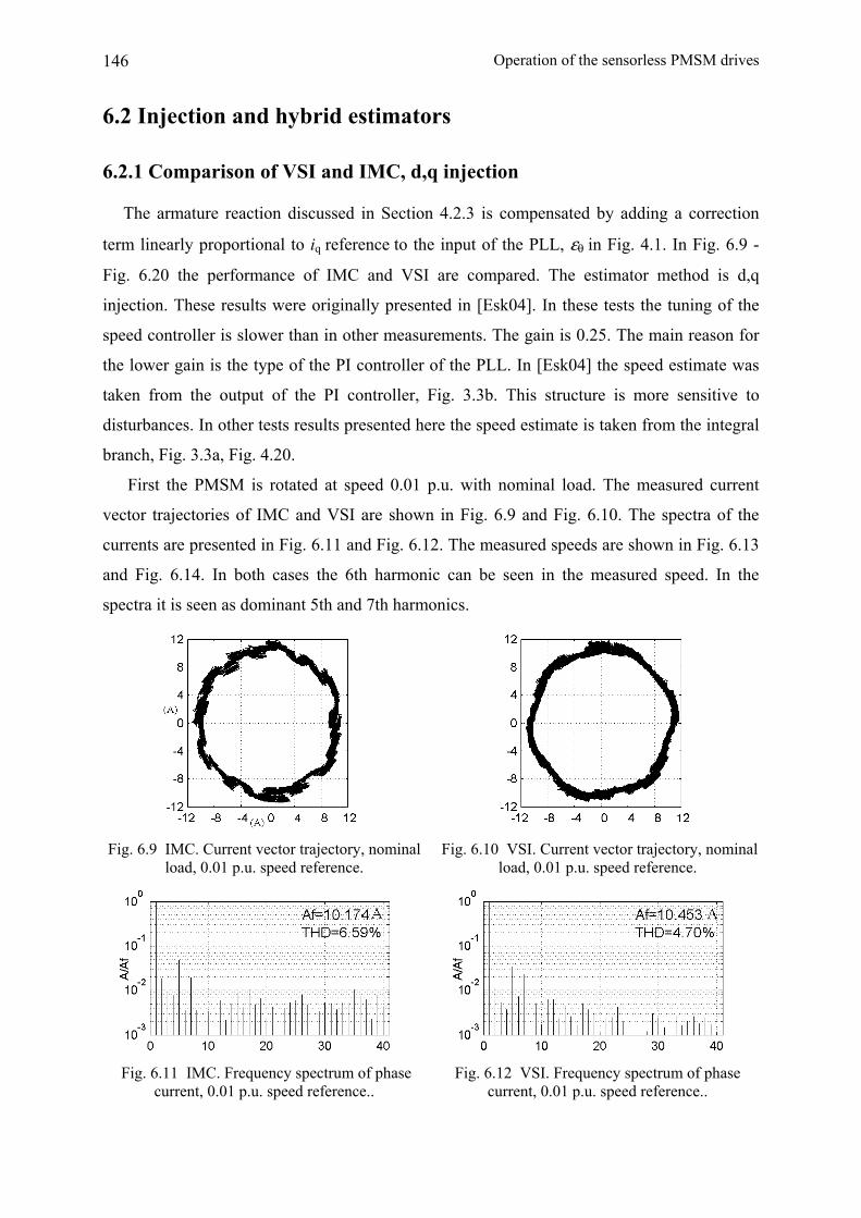
Operation of the sensorless PMSM drives 146
6.2 Injection and hybrid estimators
6.2.1 Comparison of VSI and IMC, d,q injection
The armature reaction discussed in Section 4.2.3 is compensated by adding a correction
term linearly proportional to iq reference to the input of the PLL, εθ in Fig. 4.1. In Fig. 6.9 -
Fig. 6.20 the performance of IMC and VSI are compared. The estimator method is d,q
injection. These results were originally presented in [Esk04]. In these tests the tuning of the
speed controller is slower than in other measurements. The gain is 0.25. The main reason for
the lower gain is the type of the PI controller of the PLL. In [Esk04] the speed estimate was
taken from the output of the PI controller, Fig. 3.3b. This structure is more sensitive to
disturbances. In other tests results presented here the speed estimate is taken from the integral
branch, Fig. 3.3a, Fig. 4.20.
First the PMSM is rotated at speed 0.01 p.u. with nominal load. The measured current
vector trajectories of IMC and VSI are shown in Fig. 6.9 and Fig. 6.10. The spectra of the
currents are presented in Fig. 6.11 and Fig. 6.12. The measured speeds are shown in Fig. 6.13
and Fig. 6.14. In both cases the 6th harmonic can be seen in the measured speed. In the
spectra it is seen as dominant 5th and 7th harmonics.
Fig. 6.9 IMC. Current vector trajectory, nominal
load, 0.01 p.u. speed reference. Fig. 6.10 VSI. Current vector trajectory, nominal
load, 0.01 p.u. speed reference.
Fig. 6.11 IMC. Frequency spectrum of phase
current, 0.01 p.u. speed reference.. Fig. 6.12 VSI. Frequency spectrum of phase
current, 0.01 p.u. speed reference..

147
Fig. 6.13 IMC. Measured speed, The reference is
0.01 p.u. Loas is nominal. Fig. 6.14 VSI. Measured speed. The reference is
0.01 p.u. Load is nominal.
The current produced by the IMC contains more ripple at higher frequencies than the current
of the VSI.
The d,q injection is also tested in the nominal frequency range. The current spectra and
measured speeds are shown in Fig. 6.15 - Fig. 6.18. At nominal speed the 12th harmonic is
dominant. Again the current spectrum of the matrix converter contains more harmonics of
higher order. In [Esk04] the IMC was tested in transients, too, and there was no significant
difference between the VSI and the IMC.
Fig. 6.15 IMC. Frequency spectrum of the phase
current, nominal speed (1 p.u.), nominal load. Fig. 6.16 VSI. Frequency spectrum of the phase
current, nominal speed (1 p.u.), nominal load.
Fig. 6.17 IMC. Measured speed. Nominal load. Fig. 6.18 VSI. Measured speed. Nominal load.
6.2.2 Hybrid estimator
In this section the performance of the hybrid estimator is verified. The IMC and the DMC
topologies are compared. Some measurements were also performed with the machine B. In
that case the PMSM is fed by a 50 kW VSI, Fig. 5.1.
In all tests the tuning of the speed control, current control and hybrid estimator are the
same as in the simulations, Table 4.1. In the measurements of this section the following motor
parameters are used in the estimator software.

Operation of the sensorless PMSM drives 148
Table 6.1 Parameters used in the estimator software.
Matrix converters (machine A) VSI (machine B) R (Ω) 0.95 0.25 ψm (Wb) 0.5 1.1 Ld = Lq (H) 0.01 0.0085
6.2.2.1 Steady state tests
IMC and DMC
In Fig. 6.19 - Fig. 6.24 the speed reference signal is 2% of nominal (supply frequency was
1.5 Hz). The load torque is nominal. The measured speeds are presented in Fig. 6.19 and Fig.
6.20. Position errors ( rr θθ − ) are shown in the next two figures. There is no clear difference
between the two different topologies. No load results in the case of IMC are presented in Fig.
6.23 and Fig. 6.24. The results shown in Fig. 6.19 - Fig. 6.28 are clearly better than those
presented in [Esk04], where only the d,q injection estimator was applied.
Fig. 6.19 IMC. Measured speed, speed reference
is 0.02 p.u. Load is nominal. Fig. 6.20 DMC. Measured speed, speed reference
is 0.02 p.u. Load is nominal.
Fig. 6.21 IMC. Position error, speed is 0.02 p.u. Fig. 6.22 DMC. Position error, speed is 0.02 p.u.
Fig. 6.23 IMC. Measured speed, no load. Fig. 6.24 IMC. Measured position error, no load.
The measured phase currents are presented in Fig. 6.25 (IMC) and Fig. 6.26 (DMC). Their

149
spectra are shown in Fig. 6.27 and Fig. 6.28. 5th and 7th components are the most significant
ones. The amplitudes of lower harmonics were higher in the case of the DMC.
Fig. 6.25 IMC. Phase currents, speed is 0.02 p.u
and load is nominal. Fig. 6.26 DMC. Phase currents, speed is 0.02 p.u.
and load is nominal.
Fig. 6.27 IMC. Spectrum of ia, speed is 0.02 p.u,
nominal load. Fig. 6.28 DMC. Spectrum of ia, speed is 0.02 p.u,
nominal load.
In Fig. 6.29 - Fig. 6.36 IMC and DMC are compared at the nominal operating point. The
measured speed of the IMC contains slightly more ripple but the position errors are practically
identical. The steady state position error is caused by an inductance error. Again, DMC
creates more lower harmonics.
Fig. 6.29 IMC. Measured speed, nominal load. Fig. 6.30 DMC. Measured speed, nominal load.
Fig. 6.31 IMC. Position error, nominal speed. Fig. 6.32 DMC. Position error, nominal speed.

Operation of the sensorless PMSM drives 150
Fig. 6.33 IMC, Phase currents, speed is 1 p.u. Fig. 6.34 DMC. Phase currents, speed is 1 p.u.
Fig. 6.35 IMC, spectrum of ia. Fig. 6.36 DMC. spectrum of ia.
VSI
In Fig. 6.37 - Fig. 6.40 the 50 kW VSI drive is tested in steady state with nominal load and
without load. The speed reference is 2% of nominal (supply frequency is 0.47 Hz).
The measured phase currents are presented in Fig. 6.41. The spectrum of the one phase
current is shown in Fig. 6.42. The harmonics of higher order also exists and now the 5th and
7th harmonics are not the dominant ones.
Fig. 6.37 VSI. Measured speed. Speed reference
is 0.02 p.u. Load is nominal. Fig. 6.38 VSI. Measured speed. Speed reference
is 0.02 p.u. No load.
Fig. 6.39 VSI. Position error. Load is nominal. Fig. 6.40 VSI. Position error. No load.
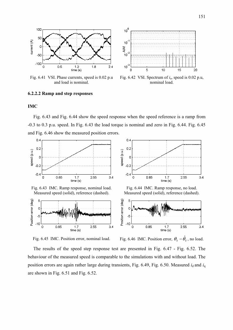
151
Fig. 6.41 VSI. Phase currents, speed is 0.02 p.u
and load is nominal. Fig. 6.42 VSI. Spectrum of ia, speed is 0.02 p.u,
nominal load.
6.2.2.2 Ramp and step responses
IMC
Fig. 6.43 and Fig. 6.44 show the speed response when the speed reference is a ramp from
-0.3 to 0.3 p.u. speed. In Fig. 6.43 the load torque is nominal and zero in Fig. 6.44. Fig. 6.45
and Fig. 6.46 show the measured position errors.
Fig. 6.43 IMC. Ramp response, nominal load.
Measured speed (solid), reference (dashed). Fig. 6.44 IMC. Ramp response, no load.
Measured speed (solid), reference (dashed).
Fig. 6.45 IMC. Position error, nominal load. Fig. 6.46 IMC. Position error, rr θθ − , no load.
The results of the speed step response test are presented in Fig. 6.47 - Fig. 6.52. The
behaviour of the measured speed is comparable to the simulations with and without load. The
position errors are again rather large during transients, Fig. 6.49, Fig. 6.50. Measured id and iq
are shown in Fig. 6.51 and Fig. 6.52.
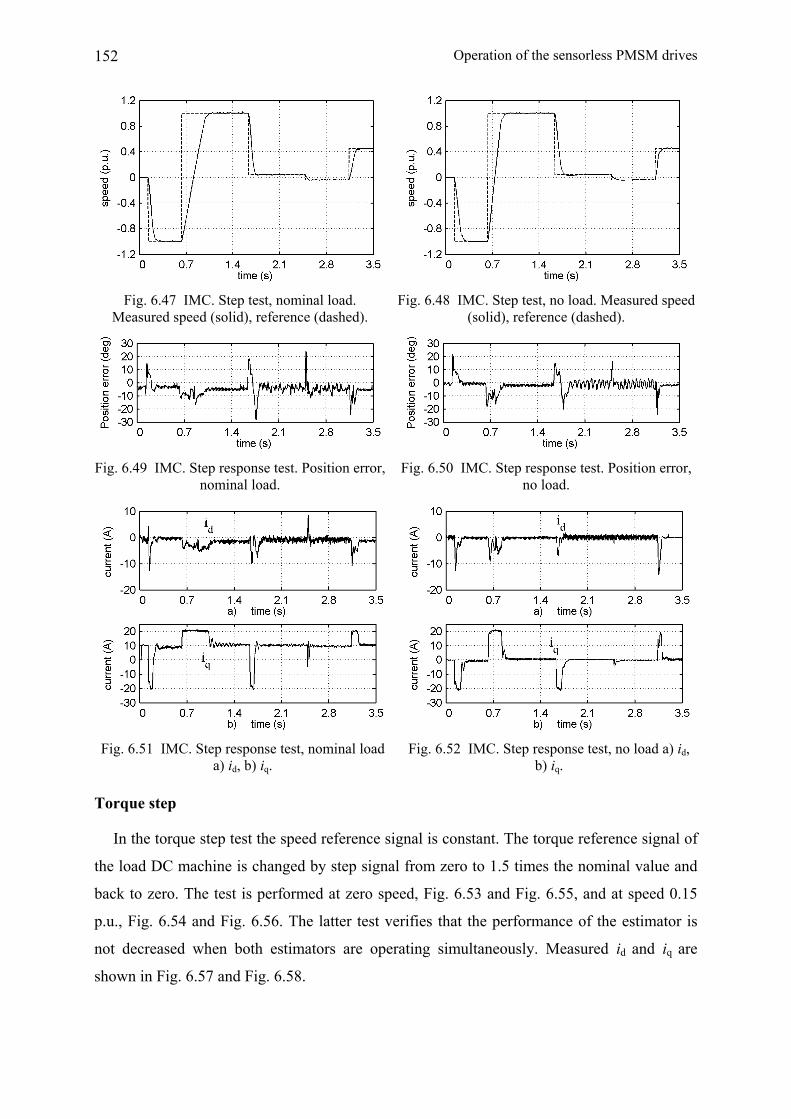
Operation of the sensorless PMSM drives 152
Fig. 6.47 IMC. Step test, nominal load.
Measured speed (solid), reference (dashed). Fig. 6.48 IMC. Step test, no load. Measured speed
(solid), reference (dashed).
Fig. 6.49 IMC. Step response test. Position error,
nominal load. Fig. 6.50 IMC. Step response test. Position error,
no load.
Fig. 6.51 IMC. Step response test, nominal load
a) id, b) iq. Fig. 6.52 IMC. Step response test, no load a) id,
b) iq.
Torque step
In the torque step test the speed reference signal is constant. The torque reference signal of
the load DC machine is changed by step signal from zero to 1.5 times the nominal value and
back to zero. The test is performed at zero speed, Fig. 6.53 and Fig. 6.55, and at speed 0.15
p.u., Fig. 6.54 and Fig. 6.56. The latter test verifies that the performance of the estimator is
not decreased when both estimators are operating simultaneously. Measured id and iq are
shown in Fig. 6.57 and Fig. 6.58.

153
Fig. 6.53 IMC, Torque step, zero speed.
Measured speed (solid), reference (dashed). Fig. 6.54 IMC, Torque step, 0.15 p.u. speed reference. Measured speed (solid), reference
(dashed).
Fig. 6.55 IMC, Torque step at zero speed.
Position error. Fig. 6.56 IMC, Torque step, 0.15 p.u. speed
reference. Position error.
Fig. 6.57 IMC, torque step at zero speed, iq and id. Fig. 6.58 IMC, torque step, 0.15 p.u. speed
reference., iq and id.
VSI
Fig. 6.59 shows the measured speed response when the speed reference is a ramp from -0.3
to 0.3 p.u. speed. The load torque is nominal. The position error is shown in Fig. 6.60.
Compared to the MCs the results are poorer. The position error is larger and the speed
fluctuates during the transient.
Motor B is magnetically more symmetric than the machine A (Appendix A). Therefore the
performance of the d,q injection is decreased. When the model based estimator operates alone
the ripple disappears.
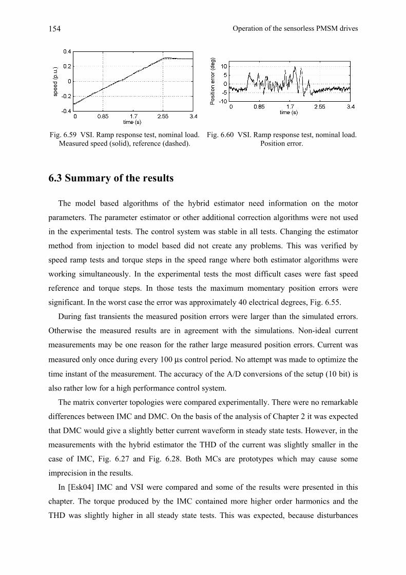
Operation of the sensorless PMSM drives 154
Fig. 6.59 VSI. Ramp response test, nominal load. Measured speed (solid), reference (dashed).
Fig. 6.60 VSI. Ramp response test, nominal load. Position error.
6.3 Summary of the results
The model based algorithms of the hybrid estimator need information on the motor
parameters. The parameter estimator or other additional correction algorithms were not used
in the experimental tests. The control system was stable in all tests. Changing the estimator
method from injection to model based did not create any problems. This was verified by
speed ramp tests and torque steps in the speed range where both estimator algorithms were
working simultaneously. In the experimental tests the most difficult cases were fast speed
reference and torque steps. In those tests the maximum momentary position errors were
significant. In the worst case the error was approximately 40 electrical degrees, Fig. 6.55.
During fast transients the measured position errors were larger than the simulated errors.
Otherwise the measured results are in agreement with the simulations. Non-ideal current
measurements may be one reason for the rather large measured position errors. Current was
measured only once during every 100 µs control period. No attempt was made to optimize the
time instant of the measurement. The accuracy of the A/D conversions of the setup (10 bit) is
also rather low for a high performance control system.
The matrix converter topologies were compared experimentally. There were no remarkable
differences between IMC and DMC. On the basis of the analysis of Chapter 2 it was expected
that DMC would give a slightly better current waveform in steady state tests. However, in the
measurements with the hybrid estimator the THD of the current was slightly smaller in the
case of IMC, Fig. 6.27 and Fig. 6.28. Both MCs are prototypes which may cause some
imprecision in the results.
In [Esk04] IMC and VSI were compared and some of the results were presented in this
chapter. The torque produced by the IMC contained more higher order harmonics and the
THD was slightly higher in all steady state tests. This was expected, because disturbances

155
between input and output are not filtered due to the absence of the DC-link with an energy
storage. In the dynamic tests the performance of IMC and VSI was similar.
The experimental results presented in Section 6.2 show that the sensorless control of the
PMSM can be realised using the proposed speed and position estimator. The system was
stable over the nominal speed range in steady state and various transient conditions. It can be
concluded from the measurements that the main drawbacks of the estimator method tested
are:
- The speed control gain must be rather low or else the disturbances generated by the
PMSM and the converter are amplified. This decreases the dynamic performance.
- The position errors may be rather large during transient. More attention should be
paid to the implementation of the hardware and the software.
Steady state at 2% speed (0.02 p.u.) and the speed reversals were tested also with the
machine B fed by the VSI. This axial flux machine is magnetically more symmetric than the
machine A. Therefore the performance was not satisfactory at low speeds where also the
signal injection was applied. When the motor was accelerated there was some oscillation in
the speed range where the model based and the injection estimators were used simultaneously,
Fig. 6.59.
The flux linkage harmonics are small compared to the machine A. In [Esk03] the machine
B was driven at low speeds using a model based estimator. The ripple in the speed and torque
was clearly smaller than in the results shown in Fig. 6.3 where the machine A was driven
using the proposed model based estimator. In [Esk03] the PMSM was succesfully decelerated
to 3% speed (0.03 p.u.) with nominal load. This test may lead to instable operation in the case
of machine A. Therefore the speed range where the d,q injection estimator is applied could be
decreased when the axial flux motor (B) is driven. These tests show that it is difficult to find
the parameters which provide an optimal performance for various machines.
PMSMs are still an emerging technology and they are not yet widely used in standard
industrial drives. Therefore it is difficult to say for what application area the performance of
the proposed estimator would be appropriate. On the basis of the experimental tests the high
performance servo drives might be too demanding, but industrial drives with moderate
dynamics are surely achievable. Such applications are, for example direct drive applications
where the PMSM is mounted directly on the rotating part of the machinery.

7 Conclusions
The vector control of synchronous machine requires knowledge of the rotor position and
angular speed. The presence of sensors measuring these quantities implies several
disadvantages in addition to the extra cost; a greater number of connections between the
motor and the control board and reduced robustness. For these reasons several strategies to
detect the speed and position without sensors have been developed over the last twenty years.
The first goal of this study was to find optimal methods to estimate the angular speed and
position of the PMSM. Requirements for a good sensorless control system were given in
Chapter 3. No modification of the basic frequency converter hardware was allowed. The
estimator should be a simple algorithm without a parameter estimator. Stable operation over
the speed range was also required.
In Chapter 3 several model based estimators (state observers, back-emf and flux linkage
estimators) were compared on the basis of a survey of the literature. The methods selected for
the comparative simulations all fulfilled the requirements excluding stable operation around
zero speed. On the basis of simulations a back-emf estimator based on the work of Matsui
was selected for experimental tests. The theory of phase locked loop was also briefly
presented in Chapter 3. This simple tracking algorithm is a basic structure of many position
and speed estimators and was also applied in this thesis.
The requirement of a stable zero speed operation was fulfilled by using the signal injection
estimator in the low speed range. Signal injection methods were analysed in Chapter 4. d,q
injection was selected because it is fairly immune to disturbances generated by the frequency
converter. The final speed and position estimator was a combination of model based back-emf
estimator and the d,q injection estimator. The injection method was used in the low speed
region and when the rotor angular speed increased, the weighting of the model based
estimator was gradually increased. The transition between the model based and the injection
estimators was explained in Chapter 4. The transition from one estimator to another was quite
a simple task because both methods had a phase locked loop structure. At the end of Chapter
4 the performance of the injection estimator and of the hybrid method were studied by
simulations.
The other goal was to study the suitability of the matrix converter for the sensorless PMSM
drives. Matrix converter topologies were presented in Chapter 2. The theory of the vector

157
modulation of the matrix converter was explained. Some non-ideal properties of the VSI and
the MCs were compared.
In Chapter 6 the performance of the proposed hybrid estimator was verified by
measurements. The PMSM was fed by the IMC and the DMC. The requirements laid down in
Chapter 3 were fulfilled. The measurements also proved that matrix converters can be used in
sensorless drives. The IMC and the DMC showed quite similar performance in all tests. The
IMC was also compared to the VSI, the widely used solution for variable speed drives. In
dynamic conditions there was no difference between the IMC and the VSI. In steady state
tests the THD of the current produced by the IMC was slightly higher. This was expected,
because the disturbances between the supply network and the output of the MC are not
filtered due to the absence of the DC-link with an energy storage. In general the low output
voltage of the matrix converters restricts their use with standard motors.
There is still work to be done if the sensorless control method presented is to be applied in
industry. More attention should be paid on the measurement of currents. A/D converters with
better accuracy should be used and several measurements during one control period should be
taken to remove the effect of single distortions. The back-emf estimator is an optimal choice
when parameters are not estimated. If parameter estimators can be applied the flux estimators
(Niemelä and Rasmussen methods or their combination) might also have a good performance.
In the measurements of this thesis the performance of the speed control was not very high.
If a faster speed control is required the effect of non-ideal properties of the PMSM and the
frequency converter should be removed more effectively.
References
[And99] G.D. Andreescu, “Position and speed sensorless control of PMSM drives based on adaptive observer,” EPE’99, Lausanne, Switzerland,1999.
[Apa03] M. Apap, J.C. Clare, P.W. Wheeler and K.J. Bradley. “Analysis and comparison of AC-AC matrix converter control strategies,” IEEE PESC’03, June 2003, Vol. 3, pp. 1287-1292.
[Ari04] A. Arias, R. Filka, G. asher and M. Sumner, “Application of the matrix converter for the sensorless control of permanent magnet AC machines using high frequency injection,” 11th international Power Electronics and Motion Control Conference, EPE-PEMC, Riga, Latvia, 2004.
[Bat00] T.D. Batzerl and K.Y. Lee, “Slotless permanent magnet syncronous motor operation without a high resolution rotor angle sensor,” IEEE Transactions on Power Conversion, Vol. 15, No. 4, December 2000, pp.366-371.
[Bla96] F. Blaschke, J. van der Burgt and A. Vandenput, “Sensorless direct field orientation at zero flux frequency,” in Proceedings of IEEE Industrial Applications Society Annual Meeting, October, 1996.
[Bol99] S. Bolognani, R. Oboe and M. Zigliotto, “Sensorless full-digital PMSM drive with EKF estimation of speed and rotor position,” IEEE Transactions on Industrial Electronics, Vol. 46, No. 1, February 1999, pp. 184-191.
[Bol01] S. Bolognani, M. Zigliotto and M. Zordan, “Extended-range PMSM sensorless speed drive based on stochastic filtering,” IEEE Transactions on Power Electronics, Vol. 16, No. 1, January 2001, pp. 110-117.
[Bol03] S. Bolognani, L. Tubiana and M. Zigliotto, “Extended Kalman filter tuning in sensorless PMSM drives,” IEEE Transactions on Industry Applications, Vol. 39, No. 6, November/December 2003, pp.1741-1747.
[Bro91] W.L. Brogan, Modern control theory, 3rd ed., Prentice-Hall, Englewood Cliffs, NJ, 1991, 653 p.
[Bru01] M. Bruckmann. O. Simon, W. Springmann, M. Münzer and M. Loddenkötter, “Application of a new IGBT module for matrix converter,” 9th European Conference on Power Application, EPE2001.
[Bur89] N. Burány, “Safe control of four-quadrant-switches,” IEEE, IAS Annual Meeting, Conference record, 1989, Vol. 1, pp. 1190-1194.
[Car03] C. Caruana, G. Asher, K. Bradley and M. Woolfson, “Flux position estimation in cage induction machines using synchronous HF injection and Kalman filtering,” IEEE Transactions on Industry Applications Vol. 39, No. 5, Sep/Oct 2003, pp.1372-1378.

159
[Cas02] D. Casadei, G. Serra, A. Tani and L. Zarri, “Matrix converter modulation strategies: a new general approach based on space-vector representation of the switch state,” IEEE Transactions on Industrial Electronics, Vol. 49, April 2002, pp. 370 – 381.
[Cha03] H.J. Cha and P.N. Enjeti, “An Approach to reduce common-mode voltage in matrix converter,” IEEE Transactions on Industry Applications, Vol. 39, No. 4, July/August 2003, pp. 1151-1159.
[Col99] F. Colamartino, C. Marchand and. A Razek, “Torque ripple minimization in permanent magnet synchronous servodrive,” IEEE Transaction on Energy Conversion, Vol. 14, No. 3, September 1999, pp. 616-621.
[Con94] A. Consoli, S. Musumeci, A. Raciti and A. Testa, “Sensorless vector and speed control of brushless motor drives,” IEEE Transactions on Industrial Electronics, Vol. 41, No. 1, February 1994, pp.91-96.
[Con00] A. Consoli, G. Scarcella and A. Testa, “A New zero frequency flux detection approach for direct field oriented control drives,” IEEE Transactions in Industry. Applications, Vol.36, No.3, May/June 2000, pp. 797 – 804.
[Con01] A. Consoli, G. Scarcella and A. Testa, “Industry application of zero-speed sensorless control techniques for PM synchronous motors,” IEEE Transactions on Industry Applications, Vol.37, No.2, March/April 2001, pp. 513-521.
[Con03] A. Consoli, G. Scarcella, “An alternative to high frequency current detection techniques for zero speed sensorless control of AC motor drives,” EPE Journal, Vol. 13, No. 3, August 2003, pp. 30 – 35.
[Cor98] M.J. Corley and R.D. Lorenz, “ Rotor position and velocity estimation for a salient-pole permanent magnet synchronous machine at standstill and high speeds,” IEEE Transactions on Industry Applications, Vol. 34 , No. 4, 1998, pp. 784 - 789.
[Deg98] M.W. Degner and R.D. Lorenz, “Using multiple saliencies for the estimation of flux, position, and velocity in AC machines,” IEEE Transactions on Industry Applications, Vol. 34, No. 5, September/October, 1998, pp. 1097-1104.
[Dha91] R. Dhaouadi, N. Mohan and L. Norum, “Design and implementation of an extended Kalman filter for the state estimation of a permanent magnet synchronous motor,” IEEE Transactions on Power Electronics, Vol. 6, No. 3, July 1991, pp. 491-497.
[Du95] T. Du, P. Vas and F. Stonach, “Design and application of extended observers for joint state and parameter estimation in high-performance AC drives,” IEE Proceedings of Electric Power Applications, Vol. 142, No. 2, March 1995, pp. 71-77.
[Elm96] C. Elmas and H.Z. De La Parra, “Application of a full-order extended Luenberger observer for a position sensorless operation of a switched reluctance motor drive,” IEE Proc.-Control Theory Applications, Vol. 143, No. 5, September 1996, pp. 401-408.
[Emp98] L. Empringham, P.W. Wheeler and J.C. Clare, “Intelligent commutation of matrix converter bi-directional switch cells using novel gate drive techniques,” IEEE, PESC’98, Conference Record, May 1998, Vol. 1, pp. 707 – 713.
[Esk02] M. Eskola, Tahtikoneen takaisinkytkemättömien säätömenetelmien vertailu, Licentiate thesis, Tampere University of Technology, Finland, 2002, 103 p.
References 160
[Esk03] M. Eskola and H. Tuusa, “Comparison of MRAS and novel simple method for position estimation in PMSM drives,” IEEE Power Electronics Specialist Conference, PESC'03, Vol. 2, June 2003, pp. 550 – 555.
[Esk04] M. Eskola, M. Jussila and H. Tuusa, “Indirect matrix converter fed PMSM -sensorless control using carrier injection,” IEEE, Power Electronics Specialists Conference, PESC’04, Aachen, Germany, 2004.
[Esk05] M. Eskola and H. Tuusa, “Sensorless control of salient pole PMSM using a low-frequency signal injection,” Conference record of EPE2005, Dresden, Germany, 2005.
[Fre96] C. French and P. Acarnley, “Control of permanent magnet motor drives using a new position estimation technique,” IEEE Transactions on Industry Applications, Vol. 32, No. 5, September/October 1996, pp. 1089-1097.
[Gre93] M.S. Grewal and A.P. Andrews, Kalman filtering, theory and practice. New Jersey, Prentice Hall, 1993, 381 p.
[Guc01] Z. Guchuan, A. Kaddouri, L-A Dessaint and O. Akhrif, “A Nonlinear state observer for the sensorless control of a permanent-magnet AC machine,” IEEE, Transactions on Industrial Electronics, Vol. 48, No. 6. December, 2001, pp. 1098-1108.
[Gyu76] L. Gyugyi and B.R. Pelly, Static power frequency changers - theory, performance, and application, A John Wiley & Sons, New York, 1976, 442 p.
[Ha99] J.-I. Ha and S.-K. Sul, “ Sensorless field orientation control of an induction machine by high frequency signal injection,” IEEE Transactions on Industry Applications, Vol. 35. No. 1, Jan./Feb. 1999.
[Har00] L. Harnefors and H.-P. Nee, “General algorithm for speed and position estimation of AC motors,” IEEE Transactions on Industrial Electronics, Vol. 47, No. 1. February 2000, pp 77-83.
[Hen94] J.R. Hendershot and T.J.E. Miller, Design of Brushless Permanent-Magnet Motors, Oxford, U.K.: Magna Physics Publishing and Clarendon Press, 1994.
[Hol96] J. Holtz and L. Springob, “Identification and compensation of torque ripple in high-precision permanent magnet motor drive,” IEEE Transactions on Industrial Electronics, Vol. 43, No. 2, April 1996, pp. 309-320.
[Hol98] J. Holtz, “Sensorless position control of induction motors -an emerging technology,” IEEE Transactions on Industrial Electronics, Vol. 45, No. 6. December, 1998 pp. 840 – 851.
[Hol02] J. Holtz and J. Quan, “Sensorless vector control of induction motors at very low speed using a nonlinear inverter model and parameter identification,” IEEE Transactions on Industry Application, Vol. 38, No. 4, July/August 2002, pp. 1087-1095.
[Hol03] D.G. Holmes and T.A. Lipo, Pulse width modulation for power converters, 2003. IEEE Press, A John Wiley & Sons, USA, 2003.
[Hsi96] G-C. Hsieh and J.C. Hung, “Phase-locked loop techniques-A survey,“ IEEE Transactions on Industrial Electronics, vol. 43, No. 6, December 1996, pp. 609-615.
161
[Hu98] J. Hu and B. Wu, “New integration algorithms for estimating motor flux over a wide speed range,” IEEE Transactions on Power Electronics, Vol. 13, No. 5, September 1998, pp. 969-977.
[Hub95] L. Huber and D. Borojević, “Space vector modulated three-phase to three-phase matrix converter with input power factor correction,” IEEE Transactions on Industry Applications, vol. 31, Nov./Dec. 1995, pp. 1234–1246.
[Iim97] K. Iimori, K. Shinohara, O. Tarumi, Z. Fu and M. Muroya, “New current controlled PWM rectifier- voltage source inverter without DC link components,” Power Conversion Conference, Nagaoka, Aug. 1997, Vol 2, pp. 783 – 786.
[Isi85] A. Isidori, Nonlinear control systems, 2nd ed., Springer-Verlag, Berlin, 1985, 479 p.
[Ito04] J-I Itoh, I. Sato, A. Odaka, H. Ohguchi, H. Kodatchi and N. Eguchi, “A novel approach to practical matrix converter motor drive system with reverse blocking IGBT,” Proceedings of Conf. Rec., IEEE PESC’04, June 2004, Vol. 3, pp. 2380 – 2385.
[Jah86] T. Jahns, G. Kliman, and T. Neumann, “Interior permanent-magnet synchronous motors for adjustable-speed drives,” IEEE Transactions on Industry Applications, vol. 22, no. 4, July/Aug. 1986, pp. 738–747.
[Jan95] P.L. Jansen and R.D. Lorenz, “Transducerless position and velocity estimation in induction and salient AC machines,” IEEE Transactions on Industry Applications, Vol. 31, No. 2, March/April 1995. pp. 204-207.
[Jan01] J.-H. Jang, J-I. Ha and S.-K. Sul, “ Vector control of surface mounted permanent magnet synchronous motor without any rotational transducer,” Proceedings of IEEE Applied Power Electronics Conference (APEC), USA, 2001.
[Jan03] J.-H. Jang, S.-K. Sul, J.-I. Ha, K. Ide and M. Sawamura, “ Sensorless drive of surface-mounted permanent-magnet motor by high-frequency signal injection based on magnetic saliency,” IEEE Transactions on Industry Applications, Volume 39, No. 4, July/August 2003, pp. 1031-1039.
[Jia97] J. Jiang and J. Holtz, “Accurate estimation of rotor position and speed of induction motor near standstill,” in Proc. IEEE Conference of Power Electronics and Drive Systems, (PEDS’97), Singapore, 1997.
[Jon89] L.A. Jones and J.H. Lang, “A state observer for the permanent-magnet synchronous motor,” IEEE Transactions on Industrial Electronics, Vol. 36, No. 3, August 1989, pp. 374-382.
[Jus03] M. Jussila, M. Salo and H. Tuusa, “Implementation of a three-phase indirect matrix converter with an indirect vector modulation method applying a microcontroller,” Proc. Conf. Rec. PCIM, 2003.
[Jus05] M. Jussila, Suoran ja epäsuoran matriisikonvertterin vertailu, Licentiate thesis, Tampere University of Technology, Finland, 2005, 116 p.
[Jus06] M. Jussila, M. Eskola and H. Tuusa, “Characteristics and comparison of output voltage non-idealities of direct and indirect matrix converters,” International Review of Electrical Engineering, IREE, Praise Worthy Prize, Volume 0, No. 0, Jan/Feb 2006, pp. 74-82.

References 162
[Ker03] T. Kereszty, V-M Leppänen and J. Luomi, “Sensorless control of surface magnet synchronous motors at low speeds using low-frequency signal injection,” Conference record of the 29th Annual Conference of the IEEE Industrial Electronics Society, IECON’03, Roanoke, VA, 2-6, November 2003.
[Kim94] J-S Kim and S-K Sul, “New stand-still position detection strategy for PMSM drive without rotational transducers,” APEC'94. Conference Proceedings, Vol 1, 13-17 February, 1994.
[Kim97] J-S Kim and S-K Sul, “New approach for high performance PMSM drives without rotational position sensors,” IEEE Transactions on Power Electronics, Vol. 12, No. 5, September 1997, pp. 904-911.
[Kim04] H. Kim, K-K Huh, R. D. Lorenz and T. M. Jahns, “A novel method for initial rotor position estimation for IPM synchronous machine drives,“ IEEE Transactions on Industry Applications, Vol. 40, No. 5, September/October 2004, pp. 1369-1378.
[Kra02] P.C. Krause, O. Wasynczuk and S.D. Sudhoff, Analysis of electric machinery and drive systems, 2nd edition, New York, IEEE Press: Wiley, 2002.
[Kol02] J.W. Kolar, M. Baumann, F. Schafmeister and H. Ertl, “Novel three-phase AC-DC-AC sparse matrix converter,” Proc. Conf. Rec. IEEE APEC, 2002, Vol. 2. pp. 777-791.
[Lee04a] J-K Lee, J-K Seok and D-C Lee, “Sensorless speed control of non-salient permanent magnet synchronous motor using rotor position tracking PI controller,” 35th annual IEEE Power Electronics Specialists Conference, Aachen, Germany, 2004. pp. 4024-4029.
[Lee04b] K-B. Lee and F. Blaabjerg, “Performance improvement of sensorless vector control for induction motor drives fed by matrix converter using nonlinear model and disturbance observer,” 35th annual IEEE Power Electronics Specialists Conference, Aachen, Germany, 2004. pp. 1341-1347.
[Lep03] V-M. Leppänen, A Low-Frequency signal-injection method for speed sensorless vector control of induction motors, Thesis for the degree of doctor of science in technology, Helsinki University of Technology, Institute of Intelligent Power Electronics, Espoo, 2003.
[Lin01] A. Lindemann, “A new IGBT with reverse blocking capability,” EPE 2001, Proc. Conf. Record, Graz, Austria 2001.
[Lin02] M. Linke, R. Kennel and J. Holtz, “Sensorless position control of permanent magnet synchronous machines without limitation at zero speed,” 28th Annual Conference of the IEEE Industrial Electronics Society IECON’02, Sevilla/Spain, Nov. 5-8, 2002.
[Lin03a] M. Linke, R. Kennel and J. Holtz, “Sensorless speed and position control of synchronous machines using alternating carrier injection,” IEEE International Electric Machines and Drives Conference IEMDC'03, Madison/Wi., USA, June 1-4, 2003.
[Lin03b] M. Linke, Injektion alternierender Trägersignale zur sensorlosen Regelung von Drehfeldmaschinen, Thesis for the degree of doctor of technology, University of Wuppertal, Germany, 2003, 103 p.

163
[Liu03] T-H. Liu, S-H. Chen and D-F. Chen, “ Design and implementation of a matrix converter PMSM drive without a shaft sensor,” IEEE Transactions on Aerospace and Electronic systems, Vol. 39, Issue 1, January 2003, pp. 228 – 243.
[Lor00] R. D. Lorentz, “Sensorless, drive control methods for stable, high performance, zero speed operation,” 9th International Conference on Power Electronics and Motion Control, EPE-PEMC, Kosice, 2000.
[Low90] T-S. Low, K.J. Tseng, T-H. Lee, K.W. Lim and K.S. Lock, “Strategy for the instantaneous torque control of permanent-magnet brushless DC drives,” IEE Proceedings, Vol. 137, Pt. B, No. 6, November 1990, pp. 355-363.
[Low93] T-S. Low, T-H. Lee and K-T. Chang, “A Nonlinear speed observer for permanent magnet synchronous motors,” IEEE Transactions on Industrial Electronics, Vol. 40, No. 3, June 1993, pp. 307-316.
[Low96] T-S. Low, C. Bi and K-T. Chang, “Motor “identity”-A Motor model for torque analysis and control,” IEEE Transactions on Industrial Electronics, Vol. 43, No. 2, April 1996, pp. 285-291.
[Lue71] D.G. Luenberger, “An Introduction to observers,” IEEE Transaction on Automatic Control, Vol. 16, No. 6, December, 1971, pp.596-602.
[Luu00] J. Luukko, Direct torque control of permanent magnet synchronous machines – analysis and implementation, Thesis for the degree of doctor of technology, Lappeenranta University of Technology, 2000, 172 p.
[Mat90] N. Matsui and M. Shigyo, “Brushless DC motor control without position and speed sensors,” IEEE Industry Applications Society, Conference Record, 1990 pp. 448 – 453.
[Mat92] N. Matsui, T Takeshita and K. Yasuda, “A new sensorless drive of brushless DC motor,” in proc. IECON’92, 1992, pp. 430-435.
[Mat96] N. Matsui, “Sensorless PM brushless DC motor drives,” IEEE Transactions on Industrial Electronics, Vol. 43, No. 2, April 1996, pp. 300-308.
[Min93] Minari, Y., Shinohara, K., Ueda, R., PWM-rectifier/voltage-source inverter without dc –link components for induction motor drive, IEE Proceedings-B – Electric power applications, vol. 140, Nov. 1993, pp. 363–368.
[Mot00] Motorola Inc., MPC555 User’s Manual, Revised 15 October 2000.
[Mun99] A.R. Muñoz and T.A. Lipo, “On-line dead-time compensation technique for open-loop PWM-VSI drives,” IEEE Transactions on Power Electronics, Vol. 14, No. 4, July 1999, pp. 683-689.
[Mur01] M. Muroya, K. Shinohara, K. Iimori, and H. Sako, “Four-step commutation strategy of PWM rectifier of converter circuit without DC link components for induction motor drives,” Proc. Conf. Rec. IEEE IEMDC, 2001, pp. 770–772.
[Nah04] B. Nahid-Mobarakeh, F. Meibody-Tabar and F-M Sargos, “Mechanical sensorless control of PMSM with online estimation of stator resistance,” IEEE Transactions on Industry Application, Vol. 40, No. 2, March/April 2004, pp. 457-471.

References 164
[Nie96] P. Nielsen, F. Blaabjerg and J.K. Pedersen, “Space vector modulated matrix converter with minimized number of switchings and a feedforward compensation of input voltage unbalance,” Proc. Conference Record, PEDES, 1996, Vol. 2, pp. 833-839.
[Nie99] M. Niemelä, Position sensorless electrically excited synchronous motor drive for industrial use based on direct flux linkage and torque control, Thesis for the degree of doctor of technology, Lappeenranta University of Technology, 1999, 144 p.
[Nov00] D.W. Novotny and T.A. Lipo, Vector control and dynamics of AC drives, Oxford, Clarendon Press, 2000.
[Oll93] J. Ollila, Analysis of PWM-converters using space vector theory-application to a voltage source rectifier, Thesis for the degree of doctor of technology, Tampere, University of Technology, Finland, 1993, 167 p.
[Orl89] T. Orlowska-Kowalska, “Application of extended Luenberger observer for flux and rotor time-constant estimation in induction motor drives,” IEE Proceedings, Vol. 136, Pt. D. No. 6, November 1989, pp. 324-330.
[Pet01] V. Petrovic, A.M. Stankovic, “Modeling of PM synchronous motors for control and estimation tasks, in Proc. of the 40th IEEE Conference on Decision and Control, Vol. 3, Dec. 2001 pp. 2229 – 2234.
[Pii04] A. Piippo, M. Hinkkanen and J. Luomi, “Sensorless control of PMM drives using a combination of voltage model and HF siganl injection,” IEEE, 39th IAS Annual Meeting, Conference Record, Vol. 2, 2004, pp. 964 – 970.
[Pii05] A. Piippo and J. Luomi, “Adaptive observer combined with HF signal injection for sensorless control of PMSM drives,” IEEE, International conference on Electric Machines and Drives, May, 2005, pp. 674 – 681.
[Pro03] A.B. Proca, A. Keyhani, A. EL-Antably, W. Lu and M. Dai, “Analytical model for permanent magnet motors with surface mounted magnets,” IEEE Transaction on Energy Conversion, Vol. 18, No. 3, September 2003, pp. 386-391.
[Qia04] W. Qian, S.K. Panda and J-X. Xu, “Torque ripple minimization in PM synchronous motors using iterative learning control,” IEEE Transactions on Power Electronics, Vol. 19, No. 2, March 2004, pp. 272-279.
[Rah04] M.F. Rahman, E. Haque, L. Tang and L. Zhong, “Problems associated with the direct torque control of an interior permanent-magnet synchronous motor drive and their remedies,” IEEE Transactions on Industrial Electronics, Vol. 51, No. 4, August 2004, pp. 799-809.
[Ras03] H. Rasmussen, P. Vadstrup and H. Borsting, “Sensorless field oriented control of a PM motor including zero speed,” in Proc. IEEE IEMDC’03, Vol. 2, Madison, USA, 2003, pp. 1224-1228.
[Rib98] L.A.S. Ribeiro, M.W. Degner, F. Briz and R.D. Lorenz, “Comparison of carrier signal voltage and current injection for the estimation of flux angle or rotor position,” Industry Applications Conference, IEEE-IAS Annual Meeting,Vol. 1, 1998.
[Rou05] M. Routimo, Digitaalisesti säädetyn rinnakkaisaktiivisuotimen virtakompensoinnin parantaminen, Licentiate thesis, Tampere University of Technology, Finland, 2005, 112 p.
165
[Row86] T. Rowan and R. Kerkman, “A new synchronous current regulator and an analysis of current regulated PWM inverters,” IEEE Transaction on Industrial Applications, Vol. 22, No. 4, July/August 1986, pp. 678-690.
[Sak01] K. Sakamoto, Y. Iwaji, T. Endo and Y. Takakura, “Position and speed sensorless control for PMSM drive using direct position error estimation,” 27. Annual Conference of the IEEE Industrial Electronics Society, Denver, USA, November, 2001, pp.1680-1685.
[Sal02] M. Salo, Microcontroller based control of current-source PWM converter applications, Thesis for the degree of doctor of technology, Tampere, University of Technology, Finland, 2002, 150 p.
[Sch88] M. Schrödl, “Detection of the rotor position of a permanent magnet synchronous machine at standstill,” proceedings of ICEM’88, Pisa, Italy, 1988.
[Sch96] M. Schrödl, “Sensorless control of AC machine at low speed and standstill based on the “INFORM” method ,” IEEE Industry Applications Conference, IAS'96, Vol. 1, 1996.
[Sch02] M. Schrödl, M. Lambeck and E. Robeischl, “Implementaltion of the INFORM method in a commercial converter for sensorless PM synchronous drives,” International Conference on Power Electronics, PCIM, 2002.
[Sep92] R.B. Sepe and J.H. Lang, “Real-time observer-based (adaptive) control of a permanent-magnet synchronous motor without mechanical sensors,” IEEE Transactions on Industry Applications, Vol. 28, No. 6, Nov/Dec 1992, pp. 1345-1352.
[Sil02] C. Silva, G. Asher and M. Sumner, “Influence of dead-time compensation on rotor position estimation in surface mounted PM machines using HF voltage injection,” Power Conversion Conference, Osaka, Japan, 2002.
[Sil03] C. Silva, G. Asher, M. Sumner, K.J. Bradley, “Sensorless control in a surface mounted PM machine using rotating injection,” EPE Journal, Vol. 13, No. 3, August 2003, pp. 12-18.
[Sol95] J. Solsona, M.I. Valla and C. Muravchik, “State estimation of a permanent magnet synchronous motor with unknown load torque,” IFAC Low Cost Automation, Buenos Aires, Argentina, 1995.
[Sol96] J. Solsona, M.I. Valla and C. Muravchik, “A nonlinear reduced order observer for permanent magnet synchronous motors,” IEEE Transactions on Industrial Electronics, Vol. 43, No. 4, August 1996, pp. 492-497.
[Sol00] J. Solsona, M.I. Valla and C. Muravchik, “Nonlinear control of a permanent magnet synchronous motor with disturbance torque estimation,” IEEE Transactions on Energy Conversion, Vol. 15, No. 2, June 2000, pp.163-168.
[Son00] J. Song, K-B Lee, J.H. Song, I. Choy and K-B Kim, “Sensorless vector control of induction motor using a novel reduced-order extended Luenberger observer,” IEEE, Industry Application Conference, Vol. 3, 2000, pp. 1828-1834.

References 166
[Sta99] C.S. Staines, G.M. Asher and K.J. Bradley, “A periodic burst injection method for deriving rotor position in saturated cage-salient induction motors without a shaft encoder,” IEEE Transactions on Industry Applications, Vol. 35, No. 4, July/August, 1999, pp. 851 – 858.
[Ste97] J.L. Stensby, Phase-locked loops: Theory and applications, Boca Raton, FL: CRC Press,1997.
[Tak86] I. Takahashi and T. Noguchi, “A new quick-response and high-efficiency control strategy of an induction machine,” IEEE Transactions on Industry Applicatations, vol. 22, September./October, 1986, pp. 820–827.
[Ued75] R. Ueda, H. Takata, S. Nakagaki and S. Takata, “On the estimation of transient state of power system by discrete nonlinear observer,” IEEE Transactions on Power Apparatus and systems, Vol. PAS-94, No. 6, Nov./Dec., 1975, pp. 2135-2140.
[Vas92] P. Vas, Electrical machines and drives, New York, Oxford University Press, 1992.
[Vas93] P. Vas, Parameter estimation, condition monitoring, and diagnosis of electrical machines, Oxford University Press, 1993, 360 p.
[Vas98] P. Vas, Sensorless vector and direct torque control, New York, Oxford University Press, 1998, 729 p.
[Vas99] P. Vas, Artificial-intelligence-based electrical machines and drives: application of fuzzy, neural, fuzzy-neural and genetic-algorithm-based techniques, Oxford University Press, 1999, 625 p.
[Ven80] M. Venturini and A. Alesina, “The generalized transformer: A new bidirectional sinusoidal waveform frequency converter with continuously adjustable input power factor,” in Proc. IEEE, PESC, 1980, pp. 242-252.
[Wal04a] O. Wallmark, L. Harnefors and O. Carlson, “Sensorless control of PMSM drives for hybrid electric vehicles,” 35th Annual IEEE Power Electronics Specialists Conference, Aachen, Germany, 2004.
[Wal04b] O. Wallmark, On Control of Permanent-Magnet Synchronous Motors in Hybrid-Electric Vehicle Applications, Licentiate thesis, Chalmers University of Technology, Sweden, 2004.
[Wal05] O. Wallmark, L. Harnefors and O. Carlson, “An improved speed and position estimator for salient permanent-magnet synchronous motors,” IEEE Transactions on industrial electronics, Vol. 52, No. 1, February 2005, pp. 255-262.
[Wei01] L. Wei and T.A. Lipo, “A novel matrix converter topology with simple commutation,” IEEE, IAS Annual Meeting, Conference Record, Volume 3, Oct. 2001, pp. 1749 – 1754.
[Whe94] P.W. Wheeler, H. Zhang and D.A. Grant, “A theoretical and practical consideration of optimised input filter design for a low loss matrix converter,” Fifth International Conference on Power Electronics and Variable-Speed Drives October 1994, pp. 363-367.
167
[Whe02] P.W. Wheeler, J. Rodríguez, J.C. Clare, L. Empringham and A. Weinstein, “Matrix converters: a technology review,” IEEE Transactions on Industrial. Electronics, vol. 49, April 2002, pp. 276–288.
[Whe04] P.W. Wheeler, J.C. Clare and L. Empringham, “Enhancement of matrix converter output waveform quality using minimized commutation times,” IEEE Transactions on Industrial Electronics, Vol. 51, Issue 1, February 2004, pp. 240 – 244.
[Wu91] R. Wu and G.R. Slemon, “A permanent magnet motor drive without a shaft sensor,” IEEE Transactions on Industry Applications, Vol. 27, No. 5, September/October 1991, pp. 1005-1011.
[Yin02] L. Ying and N. Ertugrul, “A new algorithm for indirect position estimation in permanent magnet AC motors,” IEEE, Power Electronics Specialists Conference, PESC’02, 2002.
[Yin03] L. Ying and N. Ertugrul, “A novel, robust DSP-based indirect rotor position estimation for permanent magnet AC motors without rotor saliency,” IEEE Transactions on Power Electronics, Vol. 18, No. 2, March 2003, pp. 539-546.
[You00] D. Yousfi, M. Azizi and A Saad, “Robust position and speed estimation algorithm for permanent magnet synchronous drives,” IEEE, Industry Applications Conference, Conference Record, Vol. 3, 2000, pp. 1541 – 1546.
[Åst97] K.J. Åström and B. Wittenmark, Computer controlled systems, 3rd ed. Upper Saddle River, Prentice Hall Inc., 1997, 555 p.
[Öst96] S. Östlund and M. Brokemper, “Sensorless rotor-position detection from zero to rated speed for an integrated PM synchronous motor drive,” IEEE Transactions on Industry Applications, Vol. 32, No. 5, September/October 1996, pp. 1158-1165.

168
Appendix A PMSMs used in experimental tests and simulations Machine A:
Nominal values
absolute p.u. torque 22 Nm speed 1500 rpm
phase current 7.5 A (RMS) PM flux 0.5 Wb 1
stator resistance 0.95 Ω 0.043 fundamental frequency
inductances: Ld, Lq
8 mH, 12 mH 0.18, 0.25
number of pole pairs 3 Inertia (PMSM + DC
machine) 0.04 kgm2
Machine B:
Nominal values
absolute p.u. torque 1800 Nm speed 120 rpm
phase current 60 A (RMS) PM flux 1.2 Wb 1
Stator resistance 0.3 Ω 0.14 Fundamental
frequency inductances: Ld, Lq
8.5 mH, 9.5 mH 0.6, 0.69
number of pole pairs
12
Inertia (PMSM + DC machine)
33 kgm2
Base values
Current ib = 2 In Voltage ub = ψmωn Impedance zb = ub/ib Inductance Lb = zb/ω r n
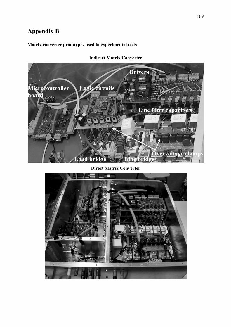
169
Appendix B Matrix converter prototypes used in experimental tests
Indirect Matrix Converter
Direct Matrix Converter

!"#$%&'# (