speech enhancement using gaussian scale mixture …papers.cnl.salk.edu/pdfs/speech enhancement using...

IEEE TRANSACTIONS ON AUDIO, SPEECH, AND LANGUAGE PROCESSING, VOL. 18, NO. 6, AUGUST 2010 1127

Speech Enhancement Using GaussianScale Mixture Models

Jiucang Hao, Te-Won Lee, Senior Member, IEEE, and Terrence J. Sejnowski, Fellow, IEEE

Abstract—This paper presents a novel probabilistic approachto speech enhancement. Instead of a deterministic logarithmicrelationship, we assume a probabilistic relationship between thefrequency coefficients and the log-spectra. The speech model inthe log-spectral domain is a Gaussian mixture model (GMM).The frequency coefficients obey a zero-mean Gaussian whosecovariance equals to the exponential of the log-spectra. Thisresults in a Gaussian scale mixture model (GSMM) for the speechsignal in the frequency domain, since the log-spectra can beregarded as scaling factors. The probabilistic relation betweenfrequency coefficients and log-spectra allows these to be treatedas two random variables, both to be estimated from the noisysignals. Expectation-maximization (EM) was used to train theGSMM and Bayesian inference was used to compute the pos-terior signal distribution. Because exact inference of this fullprobabilistic model is computationally intractable, we developedtwo approaches to enhance the efficiency: the Laplace methodand a variational approximation. The proposed methods wereapplied to enhance speech corrupted by Gaussian noise andspeech-shaped noise (SSN). For both approximations, signalsreconstructed from the estimated frequency coefficients providedhigher signal-to-noise ratio (SNR) and those reconstructed fromthe estimated log-spectra produced lower word recognition errorrate because the log-spectra fit the inputs to the recognizer better.Our algorithms effectively reduced the SSN, which algorithmsbased on spectral analysis were not able to suppress.

Index Terms—Gaussian scale mixture model (GSMM), Laplacemethod, speech enhancement, variational approximation.

I. INTRODUCTION

S PEECH enhancement improves the quality of signals cor-rupted by the adverse noise, channel distortion such as

competing speakers, background noise, car noise, room rever-berations, and low-quality microphones. A broad range of appli-cations includes mobile communications, robust speech recog-nition, low-quality audio devices, and aids for the hearing im-paired.

Although speech enhancement has attracted intensive re-search [1] and algorithms motivated from different aspects have

Manuscript received October 20, 2008; revised July 10, 2009. First publishedAugust 11, 2009; current version published July 14, 2010. The associate editorcoordinating the review of this manuscript and approving it for publication wasDr. Susanto Rahardja.

J. Hao is with the Computational Neurobiology Laboratory, Salk Institute,La Jolla, CA 92037 USA, and also with the Institute for Neural Computation,University of California, San Diego, CA 92093 USA.

T.-W. Lee is with the Qualcomm, Inc., San Diego, CA 92121 USA.T. J. Sejnowski is with the Howard Hughes Medical Institute and Computa-

tional Neurobiology Laboratory, Salk Institute, La Jolla, CA 92037 USA, andalso with the Division of Biological Sciences, University of California, SanDiego, CA 92093 USA.

Digital Object Identifier 10.1109/TASL.2009.2030012

been developed, it is still an open problem [2] because there areno precise models for both speech and noise [1]. Algorithmsbased on multiple microphones [2]–[4] and single microphonehave also been successful in achieving some measure of speechenhancement [5]–[13].

In spectral subtraction [5], the noise spectrum is subtractedto estimate the spectral magnitude which is believed to bemore important than phase for speech quality. Signal subspacemethods [6] attempt to find a projection that maps the signal andnoise onto disjoint subspaces. The ideal projection splits thesignal and noise, and the enhanced signal is constructed fromthe components that lie in the signal subspace. This approachhas been applied to single microphone source separation [14].Other speech enhancement algorithms have been based onaudio coding [15], independent component analysis (ICA) [16]and perceptual models [17].

Statistical-model-based speech enhancement systems [7]have proven to be successful. Both the speech and noise areassumed to obey random processes and treated as random vari-ables. The random processes are specified by the probabilitydensity function (pdf) and the dependency among the randomvariables is described by the conditional probabilities. Becausethe exact models for speech and noise are unknown [1], speechenhancement algorithms based on various models have beendeveloped. The short-time spectral amplitude (STSA) estimator[8] and the log-spectral amplitude estimator (LSAE) [9] use aGaussian pdf for both speech and noise in the frequency do-main, but differ in signal estimation. The STSA minimizes theminimum mean square error (MMSE) of the spectral amplitude,while the LSAE minimizes the MMSE of the log-spectrum,which is believed to be more suitable for speech processing.Hidden Markov models (HMMs) that include the temporalstructure has been developed for clean speech. An HMM withgain adaptation has been applied to the speech enhancement[18] and to the recognition of clean and noisy speech [19].Super-Gaussian priors, including Gaussian, Laplacian, andGamma densities, have been used to model the real part andimaginary part of the frequency components [10], and theMMSE estimator used for signal estimation. The log-spectra ofspeech has often been explicitly and accurately modeled by theGaussian mixture model (GMM) [11]–[13]. The GMM clusterssimilar log-spectra together and represents them by a mixturecomponent. The family of GMM has the ability to modelany distribution given a sufficient number of mixtures [20],although a small number of mixtures is often enough. However,because signal estimation is intractable, MIXMAX [11] andTaylor expansion [12], [13] are used. Speech enhancementusing the log-spectral domain models offers better spectralestimation and is more suitable for speech recognition.

1558-7916/$26.00 © 2010 IEEE

1128 IEEE TRANSACTIONS ON AUDIO, SPEECH, AND LANGUAGE PROCESSING, VOL. 18, NO. 6, AUGUST 2010

Previous models have estimated either the frequency coeffi-cients or the log-spectra, but not both. The estimated frequencycoefficients usually produced better signal quality measured bythe signal-to-noise ratio (SNR), but the estimated log-spectrausually provided lower recognition error rate, because higherSNR may not necessarily give a lower error rate. In this paper,we propose a novel approach to estimating both features atthe same time. The idea is to specify the relation betweenthe log-spectra and frequency coefficients stochastically. Wemodeled the log-spectra using a GMM following [11]–[13],where each mixture captures the spectra of similar phonemes.The frequency coefficients obey a Gaussian density whosecovariances are the exponentials of the log-spectra. This resultsin a Gaussian scale mixture model (GSMM) [21], which hasbeen applied to the time–frequency surface estimation [22],separation of of the sparse sources [23], and musical audiocoding [24]. In a probabilistic setting, both features can beestimated. An approximate EM algorithm was developed totrain the model and two approaches, the Laplace method [25]and the variational approximation [26], were used for signalestimation. The enhanced signals can be constructed fromeither the estimated frequency coefficients or the estimatedlog-spectra, depending on the applications.

This paper is organized as the follows. Section II introducesthe GSMM for the speech and the Gaussian for the noise. InSection III, an EM algorithm for parameter estimation is de-rived. Section IV presents the Laplace method and a variationalapproximation for the signal estimation. Section V shows theexperimental results and the comparisons to other algorithmsapplied to enhance the speeches corrupted by speech shapednoise (SSN) and Gaussian noise. Section VI concludes thepaper.

Notation: We use , , and to denote the time do-main signal for clean speech, noisy speech, and noise, respec-tively. The upper cases , , and denote the frequencycoefficients for frequency bin at frame . The is the log-spectrum. The is a Gaussian density for withmean and precision which is defined as the inverse ofthe variance , where is the mix-ture.

II. GAUSSIAN SCALE MIXTURE MODEL

A. Acoustic Model

Assuming additive noise, the time domain acoustic model is. After fast Fourier transform (FFT) it becomes

(1)

where denotes the frequency bin.The noise is modeled by a Gaussian

(2)

with zero mean and precision . Notethis Gaussian is of a complex variable, because the FFT coeffi-cients are complex.

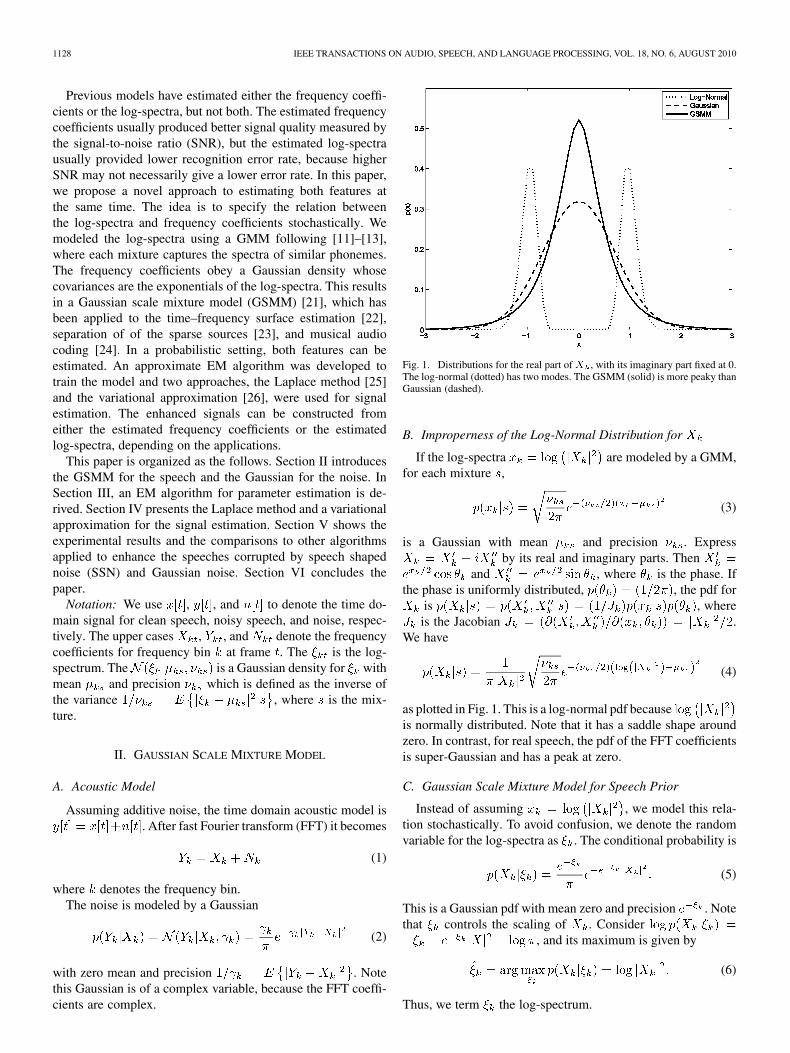
Fig. 1. Distributions for the real part of� , with its imaginary part fixed at 0.The log-normal (dotted) has two modes. The GSMM (solid) is more peaky thanGaussian (dashed).

B. Improperness of the Log-Normal Distribution for

If the log-spectra are modeled by a GMM,for each mixture ,

(3)

is a Gaussian with mean and precision . Expressby its real and imaginary parts. Then

and , where is the phase. Ifthe phase is uniformly distributed, , the pdf for

is , whereis the Jacobian .

We have

(4)

as plotted in Fig. 1. This is a log-normal pdf becauseis normally distributed. Note that it has a saddle shape aroundzero. In contrast, for real speech, the pdf of the FFT coefficientsis super-Gaussian and has a peak at zero.

C. Gaussian Scale Mixture Model for Speech Prior

Instead of assuming , we model this rela-tion stochastically. To avoid confusion, we denote the randomvariable for the log-spectra as . The conditional probability is

(5)

This is a Gaussian pdf with mean zero and precision . Notethat controls the scaling of . Consider

, and its maximum is given by

(6)

Thus, we term the log-spectrum.

HAO et al.: SPEECH ENHANCEMENT USING GSMMs 1129

The phonemes of speech have particular spectra across fre-quency. To group phonemes of similar spectra together and rep-resent them efficiently, we model the log-spectra by a GMM

(7)

(8)

where is the mixture index. Each mixture presents a templateof log-spectra, with a corresponding variability allowed for eachtemplate via the Gaussian mixture component variances. Themixture may correspond to particular phonemes with similarspectra. Though the precision for is diagonal,does not factorize over , i.e., the frequency bins are dependent.The pdf for is

(9)

which is the GSMM because controls the scaling of andobeys a GMM [21]. Note that are statisticallydependent because of the dependency among .

The GSMM has a peak at zero and is super-Gaussian [21]. Itis more peaky and has heavier tails than Gaussian, as shown inFig. 1. The GSMM, which is unimodal and super Gaussian, is aproper model for speech and has been used in audio processing[22]–[24].

III. EM ALGORITHM FOR TRAINING THE GSMM

The parameters of the GSMM, , are esti-mated from the training samples by maximum likelihood (ML)using EM algorithm [27]. The log-likelihood is

(10)

The inequality holds for any choice of distribution due toJensen’s inequality [28]. The EM algorithm iteratively opti-mizes over and . When equals the posterior distri-bution ,the lower bound is tight, . The details of theEM algorithm are given in the Appendix.

IV. TWO SIGNAL ESTIMATION APPROACHES

To recover the signal, we need the posterior pdf of the speech.However, for sophisticated models, the closed-form solutions

for the posterior pdf are difficult to obtain. To enhance thetractability, we use the Laplace method [25] and a variationalapproximation [26].

Each frame is independent and processed sequentially. Theframe index is omitted for simplicity. We rewrite the full modelas

(11)

where is given by (2), is given by (5),is a GMM given in (8) and is the mixture proba-

bility.

A. Laplace Method for Signal Estimation

The Laplace method [25] computes maximum a posteriori(MAP) estimator for each . We estimate and by maxi-mizing

(12)

For fixed , the MAP estimator for is

(13)

For fixed , the optimization over can be performed usingNewton’s method.

(14)

whereand . This updaterule is initialized by both , the means of GSMM and

, the noisy log-spectra. After iterating to con-vergence, the that gives higher value of is se-lected. Note that because is a concave function in ,

, Newton’s method works efficiently.Denote the convergent value for from (14) as and

compute using (13). We obtain the MAP estimators

(15)

Because the true is unknown, the estimators are averagedover all mixtures. The posterior mixture probability is

(16)

where . This integralis intractable. The has zero mean and variance


, and is ap-proximated by . Under thisapproximation, we have

(17)The estimated signal can be constructed from the average of

either or , weighted by the posterior mixture probability

(18)

(19)

(20)

where the phase of the noisy signal is used. The time do-main signal is synthesized by applying inverse fast Fourier trans-form (IFFT).

B. Variational Approximation for Signal Estimation

Variational approximation [26] employs a factorized poste-rior pdf. Here, we assume the posterior pdf over and con-ditioned on factorizes

(21)

The difference between and the true posterior is measured bythe Kullback–Leibler (KL)-divergence [28], , defined as

(22)where is the expectation over . Choose the optimal that isclosest to the true posterior in the sense of the KL -divergence,

.Following the derivation in [26], the optimal satisfies

(23)

As shown later in (28), we can use .Because the above equation is quadratic in , isGaussian

(24)

(25)

(26)

The optimal that minimizes is

(27)

Because this pdf is hard to work with, we use the Laplacemethod to approximate it by a Gaussian

(28)

(29)

(30)

The is chosen to be the posterior mode, , theupdate rule is

(31)

(32)

The indicates is a concave function in ,thus Newton’s method is efficient.

The variational algorithm is initialized withand . Note that in (25) can be substi-tuted into (31) and (32) to avoid redundant computation. Thenthe updates over , and iterate until convergence.

To compute the posterior mixture probability, we define

(33)

The posterior mixture probability is

(34)

(35)

The function in-creases when decreases. Because we use a Gaussian for

, is not theoretically guaranteed to increase, butit is used empirically to monitor the convergence.

With the estimated log-spectra , FFT coefficients , andposterior mixture probability , signals are constructed intwo ways given by (18) and (20). Time domain signal is syn-thesized by applying IFFT.


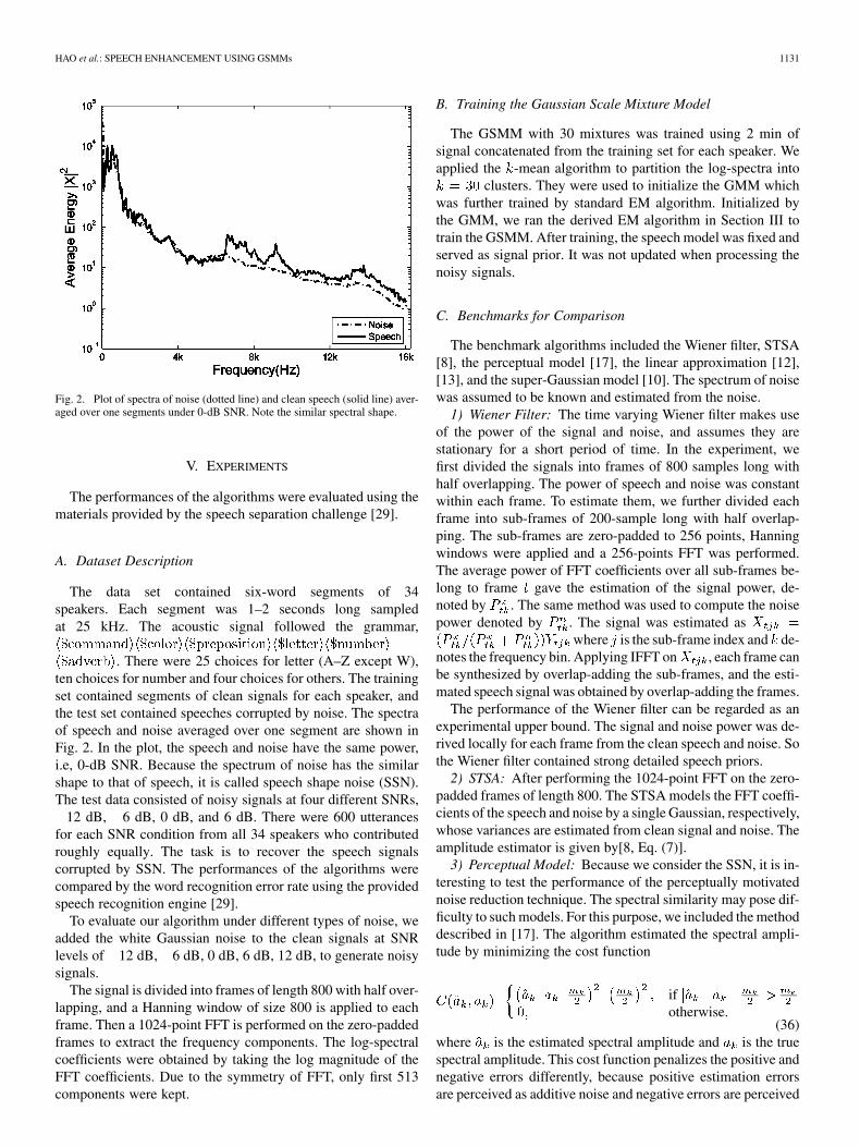
Fig. 2. Plot of spectra of noise (dotted line) and clean speech (solid line) aver-aged over one segments under 0-dB SNR. Note the similar spectral shape.

V. EXPERIMENTS

The performances of the algorithms were evaluated using thematerials provided by the speech separation challenge [29].

A. Dataset Description

The data set contained six-word segments of 34speakers. Each segment was 1–2 seconds long sampledat 25 kHz. The acoustic signal followed the grammar,

. There were 25 choices for letter (A–Z except W),ten choices for number and four choices for others. The trainingset contained segments of clean signals for each speaker, andthe test set contained speeches corrupted by noise. The spectraof speech and noise averaged over one segment are shown inFig. 2. In the plot, the speech and noise have the same power,i.e, 0-dB SNR. Because the spectrum of noise has the similarshape to that of speech, it is called speech shape noise (SSN).The test data consisted of noisy signals at four different SNRs,

12 dB, 6 dB, 0 dB, and 6 dB. There were 600 utterancesfor each SNR condition from all 34 speakers who contributedroughly equally. The task is to recover the speech signalscorrupted by SSN. The performances of the algorithms werecompared by the word recognition error rate using the providedspeech recognition engine [29].

To evaluate our algorithm under different types of noise, weadded the white Gaussian noise to the clean signals at SNRlevels of 12 dB, 6 dB, 0 dB, 6 dB, 12 dB, to generate noisysignals.

The signal is divided into frames of length 800 with half over-lapping, and a Hanning window of size 800 is applied to eachframe. Then a 1024-point FFT is performed on the zero-paddedframes to extract the frequency components. The log-spectralcoefficients were obtained by taking the log magnitude of theFFT coefficients. Due to the symmetry of FFT, only first 513components were kept.

B. Training the Gaussian Scale Mixture Model

The GSMM with 30 mixtures was trained using 2 min ofsignal concatenated from the training set for each speaker. Weapplied the -mean algorithm to partition the log-spectra into

clusters. They were used to initialize the GMM whichwas further trained by standard EM algorithm. Initialized bythe GMM, we ran the derived EM algorithm in Section III totrain the GSMM. After training, the speech model was fixed andserved as signal prior. It was not updated when processing thenoisy signals.

C. Benchmarks for Comparison

The benchmark algorithms included the Wiener filter, STSA[8], the perceptual model [17], the linear approximation [12],[13], and the super-Gaussian model [10]. The spectrum of noisewas assumed to be known and estimated from the noise.

1) Wiener Filter: The time varying Wiener filter makes useof the power of the signal and noise, and assumes they arestationary for a short period of time. In the experiment, wefirst divided the signals into frames of 800 samples long withhalf overlapping. The power of speech and noise was constantwithin each frame. To estimate them, we further divided eachframe into sub-frames of 200-sample long with half overlap-ping. The sub-frames are zero-padded to 256 points, Hanningwindows were applied and a 256-points FFT was performed.The average power of FFT coefficients over all sub-frames be-long to frame gave the estimation of the signal power, de-noted by . The same method was used to compute the noisepower denoted by . The signal was estimated as

where is the sub-frame index and de-notes the frequency bin. Applying IFFT on , each frame canbe synthesized by overlap-adding the sub-frames, and the esti-mated speech signal was obtained by overlap-adding the frames.

The performance of the Wiener filter can be regarded as anexperimental upper bound. The signal and noise power was de-rived locally for each frame from the clean speech and noise. Sothe Wiener filter contained strong detailed speech priors.

2) STSA: After performing the 1024-point FFT on the zero-padded frames of length 800. The STSA models the FFT coeffi-cients of the speech and noise by a single Gaussian, respectively,whose variances are estimated from clean signal and noise. Theamplitude estimator is given by[8, Eq. (7)].

3) Perceptual Model: Because we consider the SSN, it is in-teresting to test the performance of the perceptually motivatednoise reduction technique. The spectral similarity may pose dif-ficulty to such models. For this purpose, we included the methoddescribed in [17]. The algorithm estimated the spectral ampli-tude by minimizing the cost function

ifotherwise.

(36)where is the estimated spectral amplitude and is the truespectral amplitude. This cost function penalizes the positive andnegative errors differently, because positive estimation errorsare perceived as additive noise and negative errors are perceived


as signal attenuation [17]. Because of the stochastic property ofspeech, minimizes the expected cost function

(37)

where is the phase and is the posterior signaldistribution. Details of the algorithm can be found in [17]. TheMATLAB code is available online [30]. The original code addssynthetic white noise to the clean signal, we modified it to addSSN to corrupt a speech at different SNR levels.

4) Linear Approximation: This approach was developed in[12], [13] and worked in the log-spectral domain. It assumeda GMM for the signal log-spectra and a Gaussian for the noiselog-spectra. So the noise had a log-normal density, in contrast toGaussian noise. The relationship among the log-spectra of thesignal , the noisy signal and the noise is given by

(38)

where is an error term.However, this nonlinear relationship causes intractability. A

linear approximation was used in [12], [13] by expanding (38)around linearly. This approximation pro-vided efficient speech enhancement. The choice for can beiteratively optimized.

5) Super-Gaussian Prior: This method was developed in[10]. Let and denote the real andthe imaginary part of the signal FFT coefficients. They were pro-cessed separately and symmetrically. We consider the real partand assume obey double-sided exponential distribution

(39)

Assume the Gaussian noise with density. Here, and are the means of and ,

respectively. Let be the a priori SNR,be the real part of the noisy signal FFT coefficient. Define

, and . It wasshown in [10, Eq. (11)] that the optimal estimator for the realpart is

(40)where denotes the complementary error function. Theoptimal estimator for the imaginary part was derived analo-gously in the same manner. The FFT coefficient estimator wasgiven by .

D. Comparison Criteria

We employed two criteria to evaluate performance of all al-gorithms: SNR and word recognition error rate. In all experi-ments, the estimated time domain signals were normalizedsuch that they have the same power as the clean signals.

1) Signal-to-Noise Ratio (SNR): SNR is defined in the timedomain as

SNR (41)

where is the clean signal and is the estimated signal.2) Word Recognition Error Rate: The speech recogni-

tion engine based on the HTK package was provided on theICSLP website [29]. It extracts 39 features from the acousticwaveforms, including 12 Mel-frequency cepstral coefficients(MFCC) and the logarithmic frame energy, their velocities (MFCC) and accelerations ( MFCC). The HMM with noskipover states and two states for each phoneme was used tomodel each word. The emission probability for each state wasa GMM of 32 mixtures, of which the covariance matrices arediagonal. The grammar used in the recognizer is the same as theone shown in Section V-A. More details about the recognitionengine are provided at [29].

To compute the recognition error rate, a score ofwas assigned to each utterance depending on how many keywords (color, letter, digit) were incorrectly recognized. The av-erage word recognition error rate was the average of the scoresof all 600 testing utterances divided by 3, i.e., the percentage ofwrongly recognized key words. This was carried out for eachSNR condition.

E. Results

1) Speech Shaped Noise: We applied the algorithms to en-hance the speech corrupted by SSN at four SNR levels and com-pared them by SNR and word recognition error rate. The Wienerfiler was regarded as an experimental upper bound, because itincorporates detailed signal prior from the clean speech.

The spectrograms of female speech and male speech areshown in Figs. 3 and 4, respectively. Fig. 5 shows the outputSNR as a function of input SNR for all algorithms. The outputSNR is averaged over the 600 test segments. Fig. 6 plots theword recognition error rate.

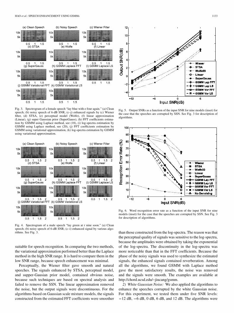
The Wiener filter outperformed other methods in low SNRconditions. This is because the power of noise and speech wascalculated locally, and it incorporated detailed prior informa-tion. The perceptual model and STSA failed to suppress the SSNbecause of the spectral similarity between the speech and thenoise. The linear approximation gave very low word recogni-tion error rate, but not superior SNR. The reason is that, using aGMM in the log-spectral domain as speech model, it reliablyestimated the log-spectrum which is a good fit to the recog-nizer input (MFCC). Because the super-Gaussian prior modeltreated the real and imaginary parts of the FFT coefficients sep-arately, it provided less accurate spectral amplitude estimationand was inferior to the linear approximation. Both the Laplacemethod and variational approximation, based on GSMM for thespeech signal, gave superior SNR for signals constructed fromthe estimated FFT coefficients and lower word recognition errorrate for signals constructed from the estimated log-spectra. Thisagreed with the expectation that frequency domain approachgave higher SNR, while log-spectral domain method was more


Fig. 3. Spectrogram of a female speech “lay blue with e four again.” (a) Cleanspeech; (b) noisy speech of 6-dB SNR; (c–j) enhanced signals by (c) Wienerfilter, (d) STSA, (e) perceptual model (Wolfe), (f) linear approximation(Linear), (g) super Gaussian prior (SuperGauss), (h) FFT coefficients estima-tion by GSMM using Laplace method, see (18), (i) log-spectra estimation byGSMM using Laplace method, see (20), (j) FFT coefficients estimation byGSMM using variational approximation, (k) log-spectra estimation by GSMMusing variational approximation.

Fig. 4. Spectrogram of a male speech “lay green at r nine soon.” (a) Cleanspeech; (b) noisy speech of 6-dB SNR; (c–i) enhanced signal by various algo-rithms. See Fig. 3.

suitable for speech recognition. In comparing the two methods,the variational approximation performed better than the Laplacemethod in the high SNR range. It is hard to compare them in thelow SNR range, because speech enhancement was minimal.

Perceptually, the Wiener filter gave smooth and naturalspeeches. The signals enhanced by STSA, perceptual model,and supper-Gausian prior model, contained obvious noise,because such techniques are based on spectral analysis andfailed to remove the SSN. The linear approximation removedthe noise, but the output signals were discontinuous. For thealgorithms based on Gaussian scale mixture models, the signalsconstructed from the estimated FFT coefficients were smoother

Fig. 5. Output SNRs as a function of the input SNR for nine models (inset) forthe case that the speeches are corrupted by SSN. See Fig. 3 for description ofalgorithms.

Fig. 6. Word recognition error rate as a function of the input SNR for ninemodels (inset) for the case that the speeches are corrupted by SSN. See Fig. 3for description of algorithms.

than those constructed from the log-spectra. The reason was thatthe perceptual quality of signals was sensitive to the log-spectra,because the amplitudes were obtained by taking the exponentialof the log-spectra. The discontinuity in the log-spectra wasmore noticeable than that in the FFT coefficients. Because thephase of the noisy signals was used to synthesize the estimatedsignals, the enhanced signals contained reverberation. Amongall the algorithms, we found GSMM with Laplace methodgave the most satisfactory results, the noise was removedand the signals were smooth. The examples are available athttp://chord.ucsd.edu/~jiucang/gsmm.

2) White Gaussian Noise: We also applied the algorithms toenhance the speeches corrupted by the white Gaussian noise.For this experiment, we tested them under five SNR levels:

12 dB, 6 dB, 0 dB, 6 dB, and 12 dB. The algorithms were


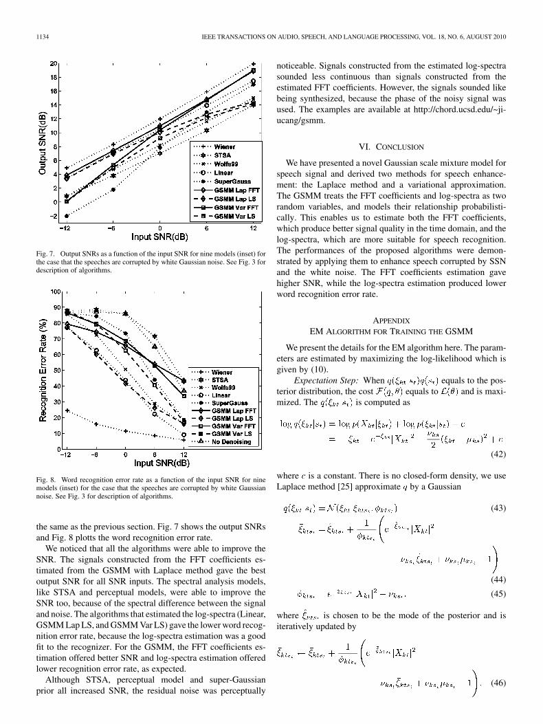
Fig. 7. Output SNRs as a function of the input SNR for nine models (inset) forthe case that the speeches are corrupted by white Gaussian noise. See Fig. 3 fordescription of algorithms.

Fig. 8. Word recognition error rate as a function of the input SNR for ninemodels (inset) for the case that the speeches are corrupted by white Gaussiannoise. See Fig. 3 for description of algorithms.

the same as the previous section. Fig. 7 shows the output SNRsand Fig. 8 plotts the word recognition error rate.

We noticed that all the algorithms were able to improve theSNR. The signals constructed from the FFT coefficients es-timated from the GSMM with Laplace method gave the bestoutput SNR for all SNR inputs. The spectral analysis models,like STSA and perceptual models, were able to improve theSNR too, because of the spectral difference between the signaland noise. The algorithms that estimated the log-spectra (Linear,GSMM Lap LS, and GSMM Var LS) gave the lower word recog-nition error rate, because the log-spectra estimation was a goodfit to the recognizer. For the GSMM, the FFT coefficients es-timation offered better SNR and log-spectra estimation offeredlower recognition error rate, as expected.

Although STSA, perceptual model and super-Gaussianprior all increased SNR, the residual noise was perceptually

noticeable. Signals constructed from the estimated log-spectrasounded less continuous than signals constructed from theestimated FFT coefficients. However, the signals sounded likebeing synthesized, because the phase of the noisy signal wasused. The examples are available at http://chord.ucsd.edu/~ji-ucang/gsmm.

VI. CONCLUSION

We have presented a novel Gaussian scale mixture model forspeech signal and derived two methods for speech enhance-ment: the Laplace method and a variational approximation.The GSMM treats the FFT coefficients and log-spectra as tworandom variables, and models their relationship probabilisti-cally. This enables us to estimate both the FFT coefficients,which produce better signal quality in the time domain, and thelog-spectra, which are more suitable for speech recognition.The performances of the proposed algorithms were demon-strated by applying them to enhance speech corrupted by SSNand the white noise. The FFT coefficients estimation gavehigher SNR, while the log-spectra estimation produced lowerword recognition error rate.

APPENDIX

EM ALGORITHM FOR TRAINING THE GSMM

We present the details for the EM algorithm here. The param-eters are estimated by maximizing the log-likelihood which isgiven by (10).

Expectation Step: When equals to the pos-terior distribution, the cost equals to and is maxi-mized. The is computed as

(42)

where is a constant. There is no closed-form density, we useLaplace method [25] approximate by a Gaussian

(43)

(44)

(45)

where is chosen to be the mode of the posterior and isiteratively updated by

(46)


This update rule is equivalent to maximizing usingthe Newton’s method

(47)

Take the derivative of with respect to and set itto zero, we can obtain the optimal . Define

(48)

Then can be obtained as

(49)

(50)

Maximization Step: The M-step optimizes over themodel parameters

(51)

(52)

(53)

The cost is computed as which can beused empirically to monitor the convergence, because theis not guaranteed to increase due to the approximation in theE-step.

The parameters of a GMM trained in the log-spectral domainare used to initialize the EM algorithm. The E-step and M-stepare iterated until convergence, which is very quick becausesimulates the log-spectra.

ACKNOWLEDGMENT

The authors would like to thank H. Attias for suggesting themodel and helpful advice on the inference algorithms. Theywould also like to thank the anonymous reviewers for valuablesuggestions.

REFERENCES

[1] Y. Ephraim and I. Cohen, “Recent advancements in speech enhance-ment,” in The Electrical Engineering Handbook. Boca Raton, FL:CRC, 2006.

[2] H. Attias, J. C. Platt, A. Acero, and L. Deng, “Speech denoising anddereverberation using probabilistic models,” in Proc. NIPS, 2000, pp.758–764.

[3] S. Gannot, D. Burshtein, and E. Weinstein, “Signal enhancement usingbeamforming and nonstationarity with applications to speech,” IEEETrans. Signal Process., vol. 49, no. 8, pp. 1614–1626, Aug. 2001.

[4] I. Cohen, S. Gannot, and B. Berdugo, “An integrated real-timebeamforming and postfiltering system for nonstationary noise environ-ments,” EURASIP J. Appl. Signal Process., vol. 11, pp. 1064–1073,2003.

[5] S. F. Boll, “Suppression of acoustic noise in speech using spectral sub-traction,” IEEE Trans. Acoust., Speech, Signal Process., vol. ASSP-27,no. 2, pp. 113–120, Apr. 1979.

[6] Y. Ephraim and H. L. V. Trees, “A signal subspace approach for speechenhancement,” IEEE Trans. Speech Audio Process., vol. 3, no. 4, pp.251–266, Jul. 1995.

[7] Y. Ephraim, “Statistical-model-based speech enhancement systems,”Proc. IEEE, vol. 80, no. 10, pp. 1526–1555, Oct. 1992.

[8] Y. Ephraim and D. Malah, “Speech enhancement using a minimummean-square error short-time spectral amplitude estimator,” IEEETrans. Acoust., Speech, Signal Process., vol. ASSP-32, no. 6, pp.1109–1121, 1984.

[9] Y. Ephraim and D. Malah, “Speech enhancement using a minimummean-square error log-spectral amplitude estimator,” IEEE Trans.Acoust., Speech, Signal Process., vol. 33, no. 2, pp. 443–445, Apr.1985.

[10] R. Martin, “Speech enhancement based on minimum mean-squareerror estimation and supergaussian priors,” IEEE Trans. Speech AudioProcess., vol. 13, no. 5, pp. 845–856, Sep. 2005.

[11] D. Burshtein and S. Gannot, “Speech enhancement using a mixture-maximum model,” IEEE Trans. Speech Audio Process., vol. 10, no. 6,pp. 341–351, Sep. 2002.

[12] B. Frey, T. Kristjansson, L. Deng, and A. Acero, “Learning dynamicnoise models from noisy speech for robust speech recognition,” in Proc.NIPS, 2001, pp. 1165–1171.

[13] T. Kristjansson and J. Hershey, “High resolution signal reconstruc-tion,” in Proc. IEEE Workshop ASRU, 2003, pp. 291–296.

[14] J. R. Hopgood and P. J. Rayner, “Single channel nonstationary sto-chastic signal separation using linear time-varying filters,” IEEE Trans.Signal Process., vol. 51, no. 7, pp. 1739–1752, Jul. 2003.

[15] A. Czyzewski and R. Krolikowski, “Noise reduction in audio signalsbased on the perceptual coding approach,” in Proc. IEEE WASPAA,1999, pp. 147–150.

[16] J.-H. Lee, H.-J. Jung, T.-W. Lee, and S.-Y. Lee, “Speech coding andnoise reduction using ica-based speech features,” in Proc. WorkshopICA, 2000, pp. 417–422.

[17] P. Wolfe and S. Godsill, “Towards a perceptually optimal spectralamplitude estimator for audio signal enhancement,” in Proc. ICASSP,2000, vol. 2, pp. 821–824.

[18] Y. Ephraim, “A Bayesian estimation approach for speech enhancementusing hidden Markov models,” IEEE Trans. Signal Process., vol. 40,no. 4, pp. 725–735, Apr. 1992.

[19] Y. Ephraim, “Gain-adapted hidden Markov models for recognition ofclean and noisy speech,” IEEE Trans. Signal Process., vol. 40, no. 6,pp. 1303–1316, Jun. 1992.

[20] C. M. Bishop, Neural Networks for Pattern Recognition. New York:Oxford Univ. Press, 1995.

[21] D. Andrews and C. Mallows, “Scale mixture of normal distributions,”J. R. Statist. Soc., vol. 36, no. 1, pp. 99–102, 1974.

[22] P. Wolfe, S. Godsill, and W. Ng, “Bayesian variable selection and reg-ularization for time-frequency surface estimation,” J. R. Statist. Soc.,vol. 66, no. 3, pp. 575–589, 2004.

[23] C. Fevotte and S. Godsill, “A Bayesian approach for blind separationof sparse sources,” IEEE Trans. Audio, Speech, Lang. Process., vol. 14,no. 6, pp. 2174–2188, Dec. 2006.

[24] E. Vincent and M. Plumbley, “Low bit-rate object coding of musicalaudio using Bayesian harmonic models,” IEEE Trans. Audio, Speech,Lang. Process., vol. 15, no. 4, pp. 1273–1282, May 2007.

[25] A. Azevedo-Filho and R. D. Shachter, “Laplace’s method approxi-mations for probabilistic inference in belief networks with continuousvariables,” in Proc. UAI, 1994, pp. 28–36.

[26] H. Attias, “A variational Bayesian framework for graphical models,”in Proc. NIPS, 2000, vol. 12, pp. 209–215.

[27] A. Dempster, N. Laird, and D. Rubin, “Maximum likelihood from in-complete data via the em algorithm,” J. R. Statist. Soc., vol. 39, no. 1,pp. 1–38, 1977.

[28] T. M. Cover and J. A. Thomas, Elements of Information Theory. NewYork: Wiley-Interscience, 1991.


[29] M. Cooke and T.-W. Lee, “Speech Separation Challenge,” [Online].Available: http://www.dcs.shef.ac.uk/~martin/SpeechSeparationChal-lenge.html

[30] P. Wolfe, “Example of Short-Time Spectral Attenuation,” [Online].Available: http://www.eecs.harvard.edu/~patrick/research/stsa.html

[31] I. Cohen, “Noise spectrum estimation in adverse environments: Im-proved minima controlled recursive averaging,” IEEE Trans. SpeechAudio Process., vol. 11, no. 5, pp. 466–475, Sep. 2003.

[32] I. Cohen and B. Berdugo, “Noise estimation by minima controlledrecursive averaging for robust speech enhancement,” IEEE SignalProcess. Lett., vol. 9, no. 1, pp. 12–15, Jan. 2002.

[33] R. McAulay and M. Malpass, “Speech enhancement using a soft-de-cision noise suppression filter,” IEEE Trans. Acoust., Speech, SignalProcess., vol. ASSP-28, no. 2, pp. 137–145, Apr. 1980.

[34] R. Martin, “Noise power spectral density estimation based on op-timal smoothing and minimum statistics,” IEEE Trans. Speech AudioProcess., vol. 9, no. 5, pp. 504–512, Jul. 2001.

[35] D. Wang and J. Lim, “The unimportance of phase in speech enhance-ment,” IEEE Trans. Acoust., Speech, Signal Process., vol. ASSP-30,no. 4, pp. 679–681, Aug. 1982.

[36] H. Attias, L. Deng, A. Acero, and J. Platt, “A new method for speechdenoising and robust speech recognition using probabilistic models forclean speech and for noise,” in Proc. Eurospeech, 2001, pp. 1903–1906.

[37] M. S. Brandstein, “On the use of explicit speech modeling in micro-phone array applications,” in Proc. ICASSP, 1998, pp. 3613–3616.

[38] L. Hong, J. Rosca, and R. Balan, “Independent component analysisbased single channel speech enhancement,” in Proc. ISSPIT, 2003, pp.522–525.

[39] C. Beaugeant and P. Scalart, “Speech enhancement using a minimumleast-squares amplitude estimator,” in Proc. IWAENC, 2001, pp.191–194.

[40] T. Lotter and P. Vary, “Noise reduction by maximum a posteriorspectral amplitude estimation with supergaussian speech modeling,”in Proc. IWAENC, 2003, pp. 83–86.

[41] C. Breithaupt and R. Martin, “Mmse estimation of magnitude-squareddft coefficoents with supergaussian priors,” in Proc. ICASSP, 2003, pp.848–851.

[42] J. Benesty, J. Chen, Y. Huang, and S. Doclo, “Study of the wiener filterfor noise reduction,” in Speech Enhancement, J. Benesty, S. Makino,and J. Chen, Eds. New York: Springer, 2005, pp. 9–42.

Jiucang Hao received the B.S. degree from the Uni-versity of Science and Technology of China (USTC),Hefei, and the M.S. degree from University of Cali-fornia at San Diego (UCSD), both in physics. He iscurrently pursuing the Ph.D. degree at UCSD.

His research interests are to develop new machinelearning algorithms and apply them to areas such asspeech enhancement, source separation, biomedicaldata analysis, etc.

Te-Won Lee (M’03–SM’06) received the M.S. de-gree and the Ph.D. degree (summa cum laude) in elec-trical engineering from the University of TechnologyBerlin, Berlin, Germany, in 1995 and 1997, respec-tively.

He was Chief Executive Officer and co-Founder ofSoftMax, Inc., a start-up company in San Diego de-veloping software for mobile devices. In December2007, SoftMax was acquired by Qualcomm, Inc., theworld leader in wireless communications where heis now a Senior Director of Technology leading the

development of advanced voice signal processing technologies. Prior to Qual-comm and SoftMax, he was a Research Professor at the Institute for NeuralComputation, University of California, San Diego, and a Collaborating Pro-fessor in the Biosystems Department, Korea Advanced Institute of Science andTechnology (KAIST). He was a Max-Planck Institute Fellow (1995–1997) anda Research Associate at the Salk Institute for Biological Studies (1997–1999).

Dr. Lee received the Erwin-Stephan Prize for excellent studies (1994) fromthe University of Technology Berlin, the Carl-Ramhauser prize (1998) for excel-lent dissertations from the DaimlerChrysler Corporation and the ICA Unsuper-vised Learning Pioneer Award (2007). In 2007, he received the SPIE ConferencePioneer Award for work on independent component analysis and unsupervisedlearning algorithms.

Terrence J. Sejnowski (SM’91–F’06) is the FrancisCrick Professor at The Salk Institute for Biolog-ical Studies where he directs the ComputationalNeurobiology Laboratory, an Investigator with theHoward Hughes Medical Institute, and a Professorof Biology and Computer Science and Engineeringat the University of California, San Diego, where heis Director of the Institute for Neural Computation.The long-range goal of his laboratory is to under-stand the computational resources of brains andto build linking principles from brain to behavior

using computational models. This goal is being pursued with a combinationof theoretical and experimental approaches at several levels of investigationranging from the biophysical level to the systems level. His laboratory hasdeveloped new methods for analyzing the sources for electrical and magneticsignals recorded from the scalp and hemodynamic signals from functionalbrain imaging by blind separation using independent components analysis(ICA). He has published over 300 scientific papers and 12 books, includingThe Computational Brain (MIT Press, 1994) with Patricia Churchland.

Dr. Sejnowski received the Wright Prize for Interdisciplinary Research in1996, the Hebb Prize from the International Neural Network Society in 1999,and the IEEE Neural Network Pioneer Award in 2002. His was elected an AAASFellow in 2006 and to the Institute of Medicine of the National Academies in2008.

speech enhancement using gaussian scale mixture …papers.cnl.salk.edu/pdfs/speech enhancement using...

Documents