Speculators, Prices and Market Volatility

Celso Brunetti Bahattin Büyükşahin Jeffrey H. Harris

Abstract

We employ data over 2005-2009 which uniquely identify categories of traders to test whether speculators like hedge funds and swap dealers cause price changes or volatility. We find little evidence that speculators destabilize financial markets. To the contrary, speculative trading activity largely reacts to market conditions and reduces volatility levels, consistent with the hypothesis that speculators provide valuable liquidity to the market. These results hold across a variety of products and suggest that hedge funds (with approximately constant risk tolerance as in Deuskar and Johnson [2010]) improve overall market quality.

Key Words: Speculation, hedge funds, swap dealers, realized volatility, price JEL Codes: C3, G1

January 6, 2011

* Brunetti: John Hopkins University, 100 International Drive, Baltimore, MD, 21202. Email: celsob@jhu.edu. Büyükşahin: International Energy Agency, Reu de la Fèdèration, 75739, Paris. Email: bahattin.buyuksahin@iea.org. Harris: University of Delaware, Newark, DE 19716, Tel: (302) 831-1812. Email: harrisj@lerner.udel.edu. We thank Kirsten Anderson, Frank Diebold, Michael Haigh, Fabio Moneta, Jim Moser, James Overdahl, David Reiffen, Michel Robe, Frank Schorfheide, seminar participants at the CFTC, the Board of Governors of the Federal Reserve System, Queen’s School of Business, the University of Delaware, the University of Mississippi, and participants at the 16th International Conference of the Society of Computational Economics for useful discussions and comments. We also thank Kirsten Soneson for excellent research assistance. The views expressed on this paper are those of the authors and do not, in any way, reflect the views or opinions of the Commodity Futures Trading Commission, its Commissioners or other Commission staff. Errors or omissions are the authors’ responsibility.

2

“The oil market, born in Texas, is behaving like a bucking bronco again. Prices that careened from $147 a barrel in mid-2008 to $31 … have jumped back to around $70 in recent days. …, politicians are again blaming speculators for this unruly behaviour.” The Economist, June 18, 2009

I. Introduction The role of speculators in financial markets has been the source of considerable

interest and controversy in recent years. As the recent financial crisis demonstrates,

failures within the financial system can have devastating effects in the real economy,

elevating concerns about the trading behavior of financial market participants, particularly

those operating outside of the public eye. The burgeoning hedge fund industry, for instance,

operates largely outside of the U.S. Securities and Exchange Commission (SEC)

jurisdiction, with few public reporting requirements. Likewise, swap dealers operate in

relatively opaque over-the-counter (OTC) markets, fueling anxiety about their influence as

well.1

Concerns about hedge fund and swap dealer trading activities also find support in

theory where noise traders, speculative bubbles and herding can drive prices away from

fundamental values and destabilize markets (see, for instance, Shleifer and Summers

[1990], de Long et al. [1990], Lux [1995] and Shiller [2003]). Conversely, traditional

speculative stabilizing theory (Friedman [1953]) suggests that profitable speculation must

involve buying when the price is low and selling when the price is high so that irrational

speculators or noise traders trading on irrelevant information will not survive in the

market place. Indeed, Deuskar and Johnson (2010) demonstrate significant gains to

supplying liquidity in the S&P 500 index futures markets.

Ultimately the question of whether these speculative groups destabilize markets or

simply supply needed liquidity becomes an empirical issue. In this paper, we analyze the

trading of both hedge funds and swap dealers in futures markets from 2005 through 2009

to test how speculative trading affects market prices and volatility. The futures markets

offer us a unique view on this question, since speculative groups are easily identified in

U.S. futures markets data and a number of futures markets have experienced significant

price fluctuations in recent years. The U.S. Commodity Futures Trading Commission

1 The 2010 Dodd-Frank financial reform legislation prescribes various oversight measures for swap dealers and requires hedge funds to register with the SEC as investment advisers. Hedge funds will provide information about their trades and portfolios as necessary to assess systemic risk.

3

(CFTC) collects daily position data from all large market participants, classifying traders by

line of business and separating commercial (hedgers) traders (like manufacturers,

producers and commercial dealers) from non-commercial (speculative) traders (like hedge

funds, floor traders and swap dealers). We specifically analyze the crude oil, natural gas,

corn, three-month Eurodollar and eMini-Dow futures markets to assess the impact of

speculative trading on market prices and volatility. Each of these markets has experienced

significant price changes during the recent financial crisis, thereby providing a unique

opportunity to examine how speculative trade affects prices and market volatility.

Importantly, futures markets have experienced significant increases in speculative

participation from both hedge funds and swap dealers during the past decade. Concurrent

with the growth in overall open interest, hedge fund participation in futures markets has

grown in recent years. Likewise, as over-the-counter financial markets have experienced

increased risk, swap dealers writing OTC contracts increasingly hedge their OTC exposure

with futures products (Büyükşahin et al. [2010]). Swap dealers also service the vast

majority of commodity index trading, a business that has grown more than 10-fold from

2003 to 2009. The increased participation of these traders has fueled claims that these

speculators destabilize markets.2 Despite these concerns, there is limited empirical

research on how speculative trading activity impacts prices and volatility (presumably since

data on speculative trading is scarce).3

We jointly examine proprietary CFTC data on speculator positions and futures

market prices. Consistent with Friedman (1953), we find that speculative activity does not

generally affect returns, but consistently reduces volatility. More specifically, we implement

multivariate Granger-causality tests examining lead-lag relations, and instrumental

variables examining contemporaneous causal relations, between daily futures market

returns and positions of the five most prominent types of market participants in each

market. Hedge fund activity does not Granger-cause any other variable in the system.

Conversely, hedge funds react to position changes of other market participants. In line with

Keynes (1923) and Deuskar and Johnson (2010), these results suggest that hedge funds

provide liquidity to the market by taking positions opposite to other market participants.

2 In fact, responding to public concerns about increased speculative positions, the CFTC has failed to increase Federal speculative position limits for many agricultural futures since 2006. 3 Indeed, even as we identify speculator positions, swap dealers and hedge funds taking apparent speculative positions may simply be hedging OTC exposures. One caveat to our analysis is that we document the effects of speculator positions, not necessarily speculation per se.

4

To assess the impact of speculative activity on risk, we construct daily realized

volatility measures from high-frequency data and run Granger-causality tests between

realized volatility and positions of the five most prominent trader categories as well.4 We

find that both swap dealer and hedge fund activities Granger-cause volatility, but as

impulse response functions demonstrate, the effect of these traders is to reduce volatility.

Additionally, we find that hedge fund and swap dealer position changes generally serve to

reduce contemporaneous market volatility. This result is of particular importance since

lower volatility implies a reduction in the overall risk of these futures markets.

Importantly, the trading activities of prominent speculators—swap dealers and hedge

funds—generally serve to stabilize prices during the most recent financial crisis, enhancing

the ability of futures markets to serve as venues for transferring risk.

Our results are robust to using herding as an alternative metric of speculative

activity as well. We explore the lead-lag relations between herding and both returns and

volatility and consistently fail to find evidence that speculative activity systematically

affects prices or volatility. Consistent with our main results based on net trader positions,

hedge fund herding is not destabilizing, but actually reduces market volatility.

Hedge fund trading has been examined during several crisis events, including the

1992 European Exchange Rate Mechanism crisis and the 1994 Mexican peso crisis (Fung

and Hsieh [2000]), the 1997 Asian financial crisis (Brown et al. [2000]), the Long Term

Capital Management financial bailout (Edwards [1999]) and the technology bubble

(Brunnermeier and Nagel [2004] and Griffin et al. [2010]). In some episodes, hedge funds

were deemed to have significant exposures which probably exerted market impact, while in

others they were unlikely to be destabilizing. In contrast to the mixed evidence on

speculation in individual markets over relatively short periods of time, our detailed data

over many markets during 2005-2009 yields the consistent results that hedge funds largely

stabilize markets.

Although our results address speculative trading more generally, the comprehensive

nature of our data speak to the value that speculators offer to the risk management

function of futures markets. In this regard, our findings comport with Hirshleifer (1989,

1990), who shows that speculation lowers hedge premia by filling the imbalance between

long and short hedging demand. Although we do not measure hedge premia directly, 4 Similarly, Büyükşahin and Harris (2010) focus on various lead-lag relations for positions and returns in the crude oil market.

5

speculative activity that reduces volatility levels will, in turn, reduce the cost of hedging.

Our analysis shows that speculators take the opposite position of hedgers and reduce

market volatility. Likewise, our results comport with Deuskar and Johnson's (2010)

supposition that investors with constant risk tolerance (e.g. hedge funds) can trade

profitably against flow-driven liquidity shocks.

Numerous studies find that futures markets tend to lead cash markets in terms of

price discovery (e.g. Hasbrouck [2003]). Our results suggest that the informative futures

market trades in these studies likely do not emanate from speculators. Rather, we find that

commercial dealer and merchant trades lead to increased volatility levels, consistent with

these traders bringing fundamental information about the underlying commodity to the

futures markets.

The remainder of the paper proceeds as follows. In section II we describe our data.

In section III we analyze contemporaneous correlation between return, volatility, and the

five most important categories of market participants in the crude oil, natural gas, corn,

three-month Eurodollars and eMini-Dow futures markets. In section IV we analyze

Granger-causality tests between trader positions and rate of return as well as positions and

volatility. In section V we analyze contemporaneous causality between volatility and

traders positions, and in section VI we measure herding and investigate whether herding

affects prices and volatility. We conclude in section VII.

II. Data Our analysis draws upon three different data sets sampled from January 3, 2005

through March 19, 2009: 1) daily futures returns; 2) high frequency transaction data for

computing realized volatility measures; and 3) daily futures positions of the most important

categories of market participants in each market.5 The New York Mercantile Exchange

(NYMEX) crude oil and natural gas contracts represent the largest energy markets, the

Chicago Board of Trade (CBOT) corn futures the largest agriculture market, the Chicago

Mercantile Exchange (CME) three-month Eurodollar futures contract is the most widely-

traded U.S. interest rate futures product, and the CBOT eMini-Dow one of the largest U.S.

equity futures markets.6

5 High frequency data for corn begins on August 1, 2006. 6 Appendix provides descriptive details about these five contracts.

6

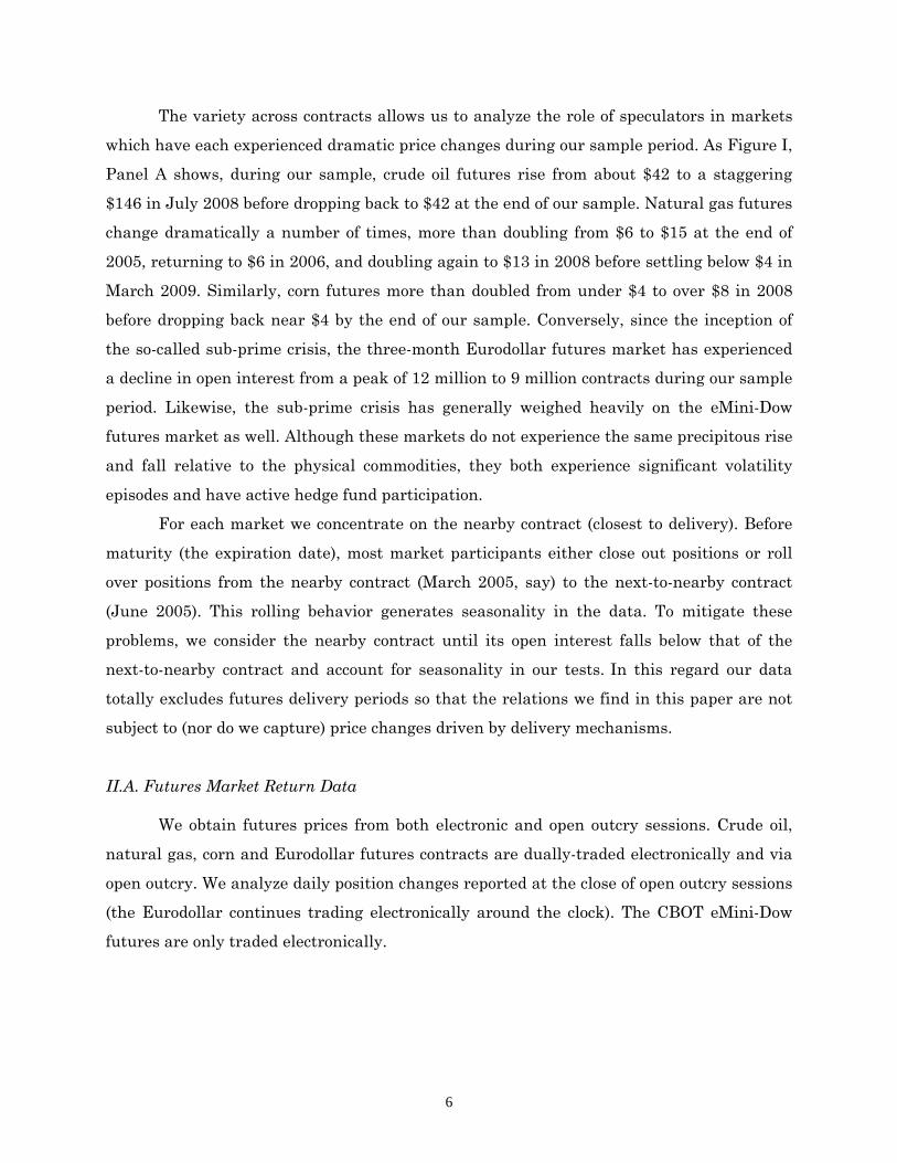
The variety across contracts allows us to analyze the role of speculators in markets

which have each experienced dramatic price changes during our sample period. As Figure I,

Panel A shows, during our sample, crude oil futures rise from about $42 to a staggering

$146 in July 2008 before dropping back to $42 at the end of our sample. Natural gas futures

change dramatically a number of times, more than doubling from $6 to $15 at the end of

2005, returning to $6 in 2006, and doubling again to $13 in 2008 before settling below $4 in

March 2009. Similarly, corn futures more than doubled from under $4 to over $8 in 2008

before dropping back near $4 by the end of our sample. Conversely, since the inception of

the so-called sub-prime crisis, the three-month Eurodollar futures market has experienced

a decline in open interest from a peak of 12 million to 9 million contracts during our sample

period. Likewise, the sub-prime crisis has generally weighed heavily on the eMini-Dow

futures market as well. Although these markets do not experience the same precipitous rise

and fall relative to the physical commodities, they both experience significant volatility

episodes and have active hedge fund participation.

For each market we concentrate on the nearby contract (closest to delivery). Before

maturity (the expiration date), most market participants either close out positions or roll

over positions from the nearby contract (March 2005, say) to the next-to-nearby contract

(June 2005). This rolling behavior generates seasonality in the data. To mitigate these

problems, we consider the nearby contract until its open interest falls below that of the

next-to-nearby contract and account for seasonality in our tests. In this regard our data

totally excludes futures delivery periods so that the relations we find in this paper are not

subject to (nor do we capture) price changes driven by delivery mechanisms.

II.A. Futures Market Return Data

We obtain futures prices from both electronic and open outcry sessions. Crude oil,

natural gas, corn and Eurodollar futures contracts are dually-traded electronically and via

open outcry. We analyze daily position changes reported at the close of open outcry sessions

(the Eurodollar continues trading electronically around the clock). The CBOT eMini-Dow

futures are only traded electronically.

7

We compute daily returns for each contract using settlement prices set daily by the

exchange at the market close.7 In particular, we construct daily returns as

)1()( −−= tptprt , where )(tp is the natural logarithm of the settlement price on day t. On

the days we switch contracts from the nearby to the next-to-nearby, both )(tp and )1( −tp

refer to the next-to-nearby contract.

The five markets we examine represent a diverse set of returns over this sample

period. Table I, column 1, reports summary statistics for returns. Daily returns on crude oil

have a negative mean (-11.6 percent annually), a positive median, high standard deviation

and mean revert. The unconditional distribution is non-Gaussian with negative skew and

kurtosis above three.8 Natural gas exhibits a significant negative mean daily returns (–47

percent annually) and a very large standard deviation (the largest of the five markets). The

unconditional distribution of the daily natural gas returns is also non-Gaussian. Corn

displays the highest average returns over the sample (6.3 percent annually). Not

surprisingly, daily Eurodollar returns average close to zero with a very low standard

deviation. Eurodollar returns also exhibit mean reversion and excess kurtosis. eMini-Dow

returns, reflecting the sub-prime crisis, have negative daily average (11 percent annually),

negative skew and excess kurtosis.

II.B. High Frequency Transaction Data and Realized Volatility

Each of these products represents very liquid markets—the median intertrade

duration for each is less than one second. From transaction data provided by the CFTC we

construct realized volatility measures. For crude oil and natural gas, we consider

transactions from both the electronic platform and the traditional pit (pit trading declined

from 100 percent to less than 30 percent of volume during our sample period). In the corn

market we only utilize electronic transactions since the vast majority of transactions occur

on the electronic platform and the intraday pit trading data contain several types of

recording errors that persist throughout our sample period, including late reports, canceled

trades, and inaccurate prices that we detect as statistical anomalies. For the Eurodollar

7 We exclude trading days abbreviated by holidays to ensure that the market is open for at least five (three for corn) trading hours. 8 For each variable in Table I we also compute skewness, kurtosis, Jarque-Bera normality tests, autocorrelation up to order 100, and augmented Dickey-Fuller non-stationarity tests. To conserve space, we only report a subset of the descriptive statistics.

8

market, we consider both electronic and pit transactions that take place when the pit is

open (and liquidity concentrates).

Realized volatility measures constructed with high frequency data can be biased by

market microstructure noise. This noise likely varies significantly over time, given the wide

range of prices experienced by these markets during our sample period. In this paper we

apply three approaches to overcome this problem and, for the sake of brevity, report only

results for the Zhang et al. (2005) two scales realized volatility (TSRV) estimator.9 The two

scales realized volatility estimator is quite simple. Let tp ∈ττ)}({ be the natural logarithm of

the price process over the time interval t, and let tba ⊂],[ be a compact interval (we use

one trading day) which is partitioned in m subintervals. For a given m, the ith intraday

subinterval is given by ],[ ,1mi

mi ττ − , where ba m

mmm =<<= τττ ...10 , and the length of each

intraday interval is given by mi

mi

mi 1−−=Δ ττ . The intraday returns are defined as

( ) ( )mi

mi

mi ppr 1−−= ττ where .,...,2,1 mi = Realized volatility on day t is the sum of squared

intraday returns sampled at frequency m.

( )2

1∑=

=m

i

mi

mt rRV (1)

Starting from the first observation, we set m=s transactions and compute RV using

equation (1).10 Then, starting from the second observation we re-compute RV using

equation (1) and iterate to the third observation, the fourth, and continue through all

available transactions for the day (with m unchanged). We then average the realized

volatility estimators obtained on the subintervals. Sampling at the relatively low frequency

dramatically reduces the effect of market microstructure noise, while the variation of the

estimates is lessened by the averaging.

We then apply equation (1) to all observations (sampling at the highest possible

frequency, m=1) to obtain a consistent estimate of the variance of the market

microstructure noise (RVall). The last step in the two scales realized volatility estimator

corrects for the bias of the noise by subtracting the noise variance from the average

estimator

9 Alternatively, the Barndorff-Nielsen et al. (2008) kernel estimator and the Andersen et al. (2001) low frequency sampling approach yield qualitatively similar results. 10 We choose the optimal sampling frequency m based on monthly volatility signature plots (Andersen et al. [2000]).

9

allt

k

j

mjt

TSRVt RVRV

kRV γ−= ∑

=1,

1 (2)

where k denotes the number of subintervals of size m and γ is the ratio between m and the

total number of observations in the trading day.

Table I, column 2, provides descriptive statistics for our realized volatility estimates.

Energy and corn markets both show a very high average volatility and a high variation in

volatility levels. This is perhaps not surprising, given that our sample is constructed to

include markets experiencing dramatic price changes. The Eurodollar market exhibits the

lowest volatility. Notably, all realized volatility measures are stationary and highly

persistent.

Figure I depicts prices and two scales realized volatility measures for our five

markets over time. Generally speaking, we see increased volatility during periods of market

decline. Crude oil, Eurodollars and equities (eMini-Dow) exhibit higher volatility in the last

part of our sample, likely linked to uncertainty about the sub-prime crisis and the

subsequent recession. Conversely, natural gas and corn exhibit relatively high variability

throughout our sample period.

II.C. Market Participant Positions

For each market we obtain individual trader positions from the CFTC’s Large

Trader Reporting System (LTRS) which identifies daily positions of individual traders

classified by line of business.11 LTRS data represents approximately 70 to 90 percent of

total open interest in each market, with the remainder comprised of small traders. The

LTRS data identifies growth in speculative positions concurrent with the dramatic swings

in prices for these commodities during our sample period. For example, hedge fund and

swap dealer positions in crude oil markets have grown 100 and 50 percent, respectively,

during our sample period.

For each market we concentrate on the five largest categories of market

participants, with hedge funds and floor brokers/traders common to all five markets. Swap

dealers are significant participants in crude oil, natural gas and corn. In these markets we

11 CFTC reporting thresholds strike a balance between effective surveillance and reporting costs with reporting thresholds during our sample period of 350 contracts for crude oil, 200 contracts for natural gas, 250 contracts for corn, 3,000 contracts for Eurodollars, and 1,000 contracts for the eMini-Dow. Aggregate LTRS data comprises the CFTC’s weekly public Commitment of Traders Reports by broad trader classifications (producer/merchants, swap dealers, managed money traders, and other non-commercials).

10

also analyze dealers/merchants (which include wholesalers, exporters/importers, shippers,

etc.) and manufacturers (for crude oil and corn, including fabricators, refiners, etc.) or

producers (for natural gas). For the Eurodollar market, we analyze commercial

arbitrageurs or broker/dealers, non-U.S. commercial banks and U.S. commercial banks. For

the eMini-Dow we analyze arbitrageurs or broker/dealers, other financial institutions, and

hedge funds that are known to be hedging (on behalf of commercial entities, for instance).

Given our focus on the effects of speculation, we specifically analyze and examine

the positions of commodity swap dealers and hedge funds. Although there is no precise

definition of hedge funds in futures markets, many hedge fund complexes are registered

with the CFTC as Commodity Pool Operators, Commodity Trading Advisors, and/or

Associated Persons who may control customer accounts. CFTC market surveillance staff

also identifies other participants who are known to be managing money. Accordingly, we

define hedge funds to include these four categories.12

As noted above, commodity swap dealers use derivative markets to manage price

exposure from OTC swaps and transactions with commodity index funds. Index funds are

increasingly used by large institutions to diversify portfolios with commodities—by June

2008, the notional value of commodity index investments tied to U.S. futures exchanges

exceeded $160 billion. These funds hold significant long-only positions, primarily in near-

term futures contracts.

For each market, we consider the number of contracts held in long (or short)

positions, the net futures positions (futures long minus futures short), and net total

positions (the sum of net futures positions and the net, delta-adjusted, option positions) of

each trader category. Columns three through seven in Table I show descriptive statistics for

changes in the net futures positions for each market participant category organized by

market. We emphasize position changes as measures of trading activity. In crude oil,

natural gas and corn markets, where swap dealers are most active, both mean and median

swap dealer position changes are negative, indicating an overall reduction in their

positions. Likewise, across all markets, hedge fund position changes are negative over our

sample period as well. The standard deviation of position changes among both swap dealers

and hedge funds is very high, indicating that these groups change positions often and/or by

large amount (as might be expected from speculative trading groups). 12 For completeness, we verify the funds in these four categories are indeed hedge funds with characterizations of these funds in the press.

11

Table II shows the five trader categories in each market comprise at least half and

up to four-fifths of the total open interest in each market. The participation rate of each

trader category varies by long and short position. Merchants, producers and manufacturers

are primarily short, consistent with the needs of these market participants to hedge long

positions in the underlying commodity. Swap dealers hold an average of 40 percent of long

positions in crude oil, natural gas and corn, consistent with large long positions taken on

behalf of commodity index funds. Interestingly, hedge funds hold large positions on both the

long and short sides of all five markets, suggesting that hedge fund activity is more

heterogeneous than other trader categories.

III. Unconditional Contemporaneous Correlations We first examine the link between trader positions and both returns and volatility

with an analysis of the correlation coefficients. Table III reports correlation coefficients

between returns and volatility, and change in positions. Merchant positions are negatively

correlated with the returns of crude oil, natural gas and corn, and positively correlated with

natural gas volatility.

Examining speculators, we find no evidence of a contemporaneous link between

swap dealer positions and returns. Swap dealer activity is positively linked to crude oil

volatility but negatively linked to natural gas volatility. Hedge fund position changes are

positively correlated with returns. However, hedge fund activity is not significantly

correlated with volatility. Hedge fund and swap dealer position changes are generally

negatively correlated with other trader positions, suggesting that both of these speculative

trader groups provide liquidity to other market participants.

The simple correlation analysis provides three main results. First, swap dealer

activity is largely unrelated to returns and volatility. Second, hedge fund activity is

positively correlated with returns but uncorrelated with volatility. Third, the correlation

between position changes of hedge funds and swap dealers with other market participants

is always negative. Speculators, by taking positions opposite to hedgers, serve to provide

liquidity in derivatives markets.

12

IV. Do Trader Position Changes Granger-Cause Returns or

Volatility? Although suggestive, correlation analysis does not establish any causal or lead/lag

relation between trader position changes and either returns or volatility. We formally test

for Granger causality between position changes and both returns and volatility in the

context of Vector Autoregressive (VAR) models using Generalized Method of Moments

(GMM) with Newey-West robust standard errors.13 Although we only report results for the

optimal lag-length in each specification, these results are robust and hold regardless of the

lag structure in the VAR.14

IV.A. Returns and Trader Position Changes

We are particularly interested in testing whether swap dealer and hedge fund

activity Granger-cause returns and/or volatility, but to better characterize the dynamics of

these markets we also present tests for the interactions among trader groups. For brevity

we do not include all parameters in the model, but rather focus on the significance of the

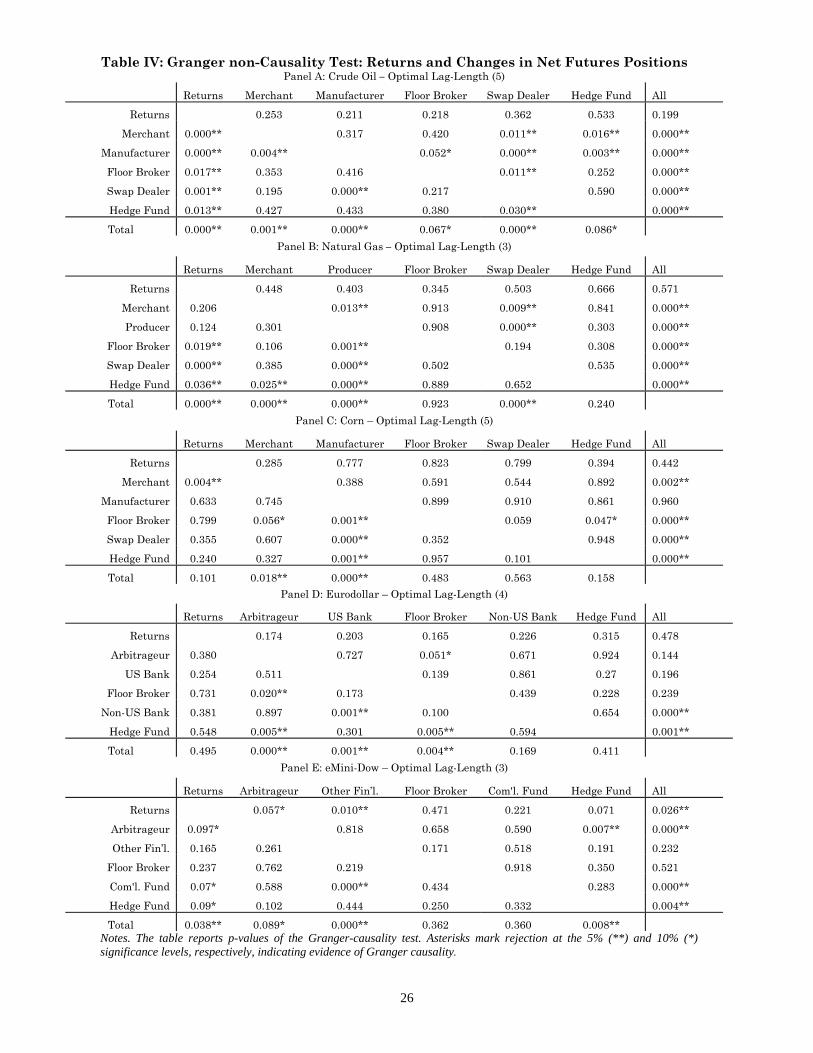
Granger causality tests. Tables IV and V provide p-values for Granger-non-causality tests

in both directions. In the upper right quadrant (column titled ‘All’) we test whether each

variable is Granger-caused by all the other variables in the system. In the lower quadrant

(row titled ‘Total’) we test whether each variable Granger-causes any other variable in the

system. The null hypothesis is that of Granger-non-causality—i.e. a p-value greater than

five percent indicates failure to reject the null. Where we find evidence that trader position

changes Granger-cause either returns or volatility, we provide impulse-response results in

Figures II and III.

Table IV presents Granger-causality tests between returns and position changes for

each of the five markets. Panel A presents results for crude oil. Returns on the crude oil

market are not Granger-caused by collective position changes of these traders (p-

value=0.199), nor by any individual trader group. On the other hand, prior returns strongly

Granger-cause positions of each individual trader group and of the full set of traders (p-

value=0.000). Hedge funds do appear to be unique in that hedge funds are the only group 13 We find no evidence of cointegrating vectors between variables used in the VAR for Granger non-causality tests. For brevity, we only report results for net futures positions but results are qualitatively similar for long futures positions, short futures positions and net total (futures and options) positions. Results for levels are nearly identical. 14 Given heteroskedasticity and serial correlation, we use Wald tests rather than Akaike (AIC) or Schwartz Information Criteria (SIC) to select the optimal lag-length (which always exceeds that selected by AIC and SIC).

13

which does not jointly Granger-cause (at 5 percent significance level) any other variable in

the system. This implies that hedge fund activity does not provide any useful information

for predicting either returns or the positions of other traders at the one day horizon.

Conversely, hedge fund activity is Granger-caused by the system (p-value=0.000). Swap

dealer activity, on the other hand, both Granger-causes and is Granger-caused by the other

variables in the system.

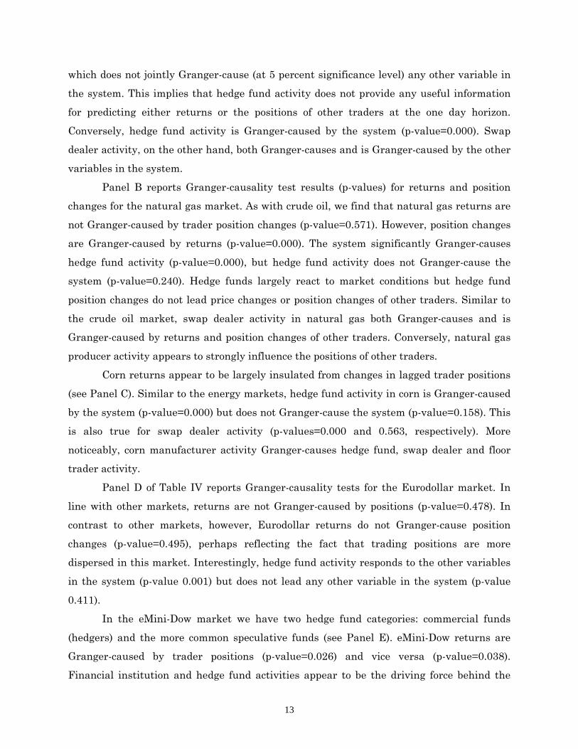
Panel B reports Granger-causality test results (p-values) for returns and position

changes for the natural gas market. As with crude oil, we find that natural gas returns are

not Granger-caused by trader position changes (p-value=0.571). However, position changes

are Granger-caused by returns (p-value=0.000). The system significantly Granger-causes

hedge fund activity (p-value=0.000), but hedge fund activity does not Granger-cause the

system (p-value=0.240). Hedge funds largely react to market conditions but hedge fund

position changes do not lead price changes or position changes of other traders. Similar to

the crude oil market, swap dealer activity in natural gas both Granger-causes and is

Granger-caused by returns and position changes of other traders. Conversely, natural gas

producer activity appears to strongly influence the positions of other traders.

Corn returns appear to be largely insulated from changes in lagged trader positions

(see Panel C). Similar to the energy markets, hedge fund activity in corn is Granger-caused

by the system (p-value=0.000) but does not Granger-cause the system (p-value=0.158). This

is also true for swap dealer activity (p-values=0.000 and 0.563, respectively). More

noticeably, corn manufacturer activity Granger-causes hedge fund, swap dealer and floor

trader activity.

Panel D of Table IV reports Granger-causality tests for the Eurodollar market. In

line with other markets, returns are not Granger-caused by positions (p-value=0.478). In

contrast to other markets, however, Eurodollar returns do not Granger-cause position

changes (p-value=0.495), perhaps reflecting the fact that trading positions are more

dispersed in this market. Interestingly, hedge fund activity responds to the other variables

in the system (p-value 0.001) but does not lead any other variable in the system (p-value

0.411).

In the eMini-Dow market we have two hedge fund categories: commercial funds

(hedgers) and the more common speculative funds (see Panel E). eMini-Dow returns are

Granger-caused by trader positions (p-value=0.026) and vice versa (p-value=0.038).

Financial institution and hedge fund activities appear to be the driving force behind the

14

connection between position changes and returns in the eMini-Dow market. Interestingly,

commercial fund activity does not significantly lead eMini-Dow returns. However, hedge

fund activity significantly leads the system of returns and other trader positions (p-

value=0.008).

To further explore how hedge fund and other trader position changes affect eMini-

Dow returns, we compute impulse-responses depicting the 10-day return response to a one

standard deviation innovation in position changes.15 As Figure II shows, the trading

activity of speculative hedge funds and dealer/arbitrageurs contribute to reversing the

negative trend in the eMini-Dow returns over our sample period. That is, although hedge

fund position changes lead price changes, the effect of net hedge fund purchases is not to

Granger-cause price increases, but rather to temper price declines. On the other hand,

other financial institutions and floor broker/trader activities appear to contribute to the

negative trend in stock returns during our sample period.16

IV.B. Volatility and Trader Position Changes

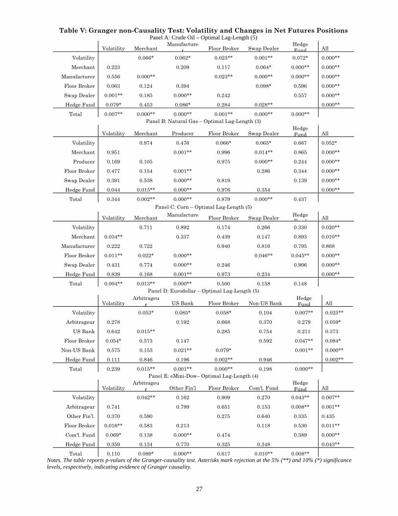
Table V reports Granger-causality tests for volatility and trader position changes.

For volatility, we use the logarithmic two scales realized volatility measure in transaction

time (described in Section II).17 Panel A shows that position changes (p-value=0.000)

Granger-cause volatility in the crude oil market. There is also a feedback effect from

volatility to trader position changes (p-value=0.007). Both swap dealer and hedge fund

position changes appear to lead volatility in the crude oil market.

Panel B of Table V reports results for the natural gas market. Natural gas volatility

is marginally (at 10 percent level) Granger-caused by trader activity (p-value=0.052), but

trader activity is not Granger-caused by volatility (p-value=0.344). Merchants, producer

and swap dealer position changes significantly lead changes in other variables in the

system, with the strongest connection between trader positions rather than with volatility.

In fact, all other trader position changes strongly lag position changes of natural gas

15 We follow Pesaran and Shin's (1998) generalized impulse responses which are invariant to the ordering of the VAR variables and do not require shocks to be orthogonal. Impulse responses generated with Cholesky decompositions with several variable orderings are similar. Response standard errors are computed with 1,000 Monte Carlo replications. 16 These results also hold separately during the run-up in the eMini-Dow (January 2005 – August 2007) and through the eMini-Dow decline (September 2007 – March 2009). 17 We confirm that logarithmic realized standard deviation is approximately Gaussian (see Andersen et al. [2003]). Our results are robust to alternative realized volatility measures as well.

15

producers. As with our results examining returns above, hedge fund activity is largely

unrelated to volatility or other trader position changes in the natural gas market.

For the corn market (Panel C) we find evidence of two-way Granger-causality

between trader position changes and volatility. Swap dealer and hedge fund activity do not

Granger-cause the system (p-values=0.158 and 0.148, respectively), but their activity

significantly lags other variables in the system (p-value=0.000 for both). As with the

analysis of returns above, manufacturer position changes significantly lead the position

changes of both swap dealers and hedge funds in the corn market.

Volatility in the Eurodollar market (Panel D) is Granger-caused by trading activity

(p-value=0.025), with the strongest link to hedge funds (p-value=0.007). In fact, hedge fund

position changes also strongly lead position changes of both non-U.S. banks and brokers.

Broker activity feeds back to hedge fund position changes as well (p-value=0.002). Overall,

however, Eurodollar volatility shows no sign of Granger-causing the position changes of

traders in this market (p-value=0.239).

Similar to most other markets eMini-Dow volatility is Granger-caused by the full set

of trader position changes (p-value=0.007) but there is evidence of only a marginal feed-

back effect (p-value=0.110). Notably, eMini-Dow volatility is also significantly led by

arbitrageur and speculative hedge fund position changes (p-values=0.042 and 0.043,

respectively). Hedge fund activity also significantly leads arbitrageur position changes.

Given the consistent connection between trader position changes and volatility, we

present impulse-responses for each market in Figure III. We are particularly interested in

the response of volatility to a shock to commodity swap dealer and hedge fund activity

shown in the two graphs to the far right. An unexpected positive shock to swap dealer

positions is associated with a significant reduction of volatility in the crude oil and natural

gas markets (Panels A and B) and a marginal reduction of volatility in the corn market

(Panel C). Likewise, an unexpected one-standard deviation increase in hedge fund activity

significantly reduces volatility in the crude oil (Panel A) and eMini-Dow (Panel E) markets

and marginally reduces volatility in the corn (Panel C) and the Eurodollar (Panel D)

markets. These facts provide further evidence that speculators generally do not destabilize

markets, but rather serve to buffet volatility brought to bear by other traders.

In fact, these impulse-response functions demonstrate that shocks to merchant

(hedger) position changes have a positive impact on volatility in crude oil and natural gas

markets. Likewise, an unexpected increase in financial institution activity also increases

16

volatility in the eMini-Dow market. These results are perhaps not surprising, since

commercial traders are commonly thought to bring fundamental information about the

commodity to the futures market, information that would thus generate higher volatility.

It is interesting to contrast the impulse responses for the eMini-Dow presented in

Figures II and III. Hedge funds and arbitrageurs that change positions against the return

trend (Figure II) are the same traders which significantly reduce market volatility (Figure

III, Panel E). Conversely, financial institutions and floor traders that trade with the return

trend have a short-term, positive effect on volatility.

Our analysis of Granger-causality suggests that speculation does not destabilize

prices across a variety of markets during historically volatile times. Although Granger-

causality tests have limitations our results are very robust, holding for both position levels

and changes, various volatility measures, and in numerous VAR specifications.

V. Contemporaneous Volatility and Trader Position Changes The above Granger-causality tests are based on a precise temporal structure: we test

whether a variable on day t helps predicting another variable the next day, t+1. However,

given that these markets are very liquid and active, it is perhaps likely that position

changes and volatility occur contemporaneously. To explore this possibility we test for a

contemporaneous causal relation between realized volatility and trader positions with the

following equation:

, , |∆ , , | ∑ , , , (1)

where RVi,t is the (log) two scales realized volatility in market i at time t, |ΔTPi,j,t| is the

(absolute value of the) trading position changes of trader group j in market i at time t, εi,t is

an error term assumed to be uncorrelated with lag values of realized volatility but not

necessarily with |ΔTPi,j,t|. The large number of lags of RVi,t covers the trading days of the

past month.

We are particularly interested in the parameter β which measures the

contemporaneous impact of trading activity on volatility. However, |ΔTPi,j,t| and εi,t may be

correlated because position changes may be endogenous. For instance, high volatility may

induce speculators to change positions so that simple OLS estimates of β may be biased. To

overcome this problem we adopt a set of instruments which are correlated with |ΔTPi,j,t|

but uncorrelated with εi,t. The instrument we propose is the change in the number of

17

traders reporting position changes, by group, in each market each day, ∆NTi,j,t. We test the

validity of the instruments with an F-test using Stock and Yogo (2005) critical values and

then estimate Equation (1) using Limited Information Maximum Likelihood (LIML).18

Table VI reports estimation results for the instrumental variable regressions. These

results are in line with the Granger-causality tests above. Interestingly merchant activity

increases volatility in the crude oil and natural gas markets (but not in corn). These effects

are economically significant. In fact, a unit change in merchant positions increases

volatility by 38 and 23 basis points in the crude oil and natural gas markets, respectively.

Likewise, floor broker activity increases volatility by 25 basis points in crude oil and four

basis points in the eMini-Dow market. Financial institution activity also increases volatility

by four basis points in the eMini-Dow market.

Notably, swap dealer activity is largely unrelated to contemporaneous volatility. More

importantly, perhaps, is the fact that a unit change in hedge fund activity reduces crude oil

volatility by 40 basis points, reduces natural gas volatility by 7 basis points, and reduces

eMini-Dow volatility by 13 basis points. We find little evidence that hedge fund activity

destabilizes these markets, but rather reduces contemporaneous volatility in futures

markets.

VI. Herding as an Alternative Speculation Metric The aggregation of speculative positions by hedge fund and commodity index trader

groupings might obscure the impact of individual traders within the group. That is, since

we measure aggregate positions by trader group, the results above do not distinguish

between a market with many traders going long (short) and a market with one dominant

long (short) position that influences the net long (short) position of the group. To

disentangle the effects of one dominant trader from a group of traders on the same side of

the market, we calculate the herding measure developed by Lakonishok et al. (1992). In

this regard, we explore whether our results reflect speculator behavior more generally, or

perhaps reflect the activity of a dominant speculator. We consider the herding metric an

alternative measure of speculative activity that excludes effects of a dominant trader.

18 LIML is less sensitive to weak instruments than two-stage least squares estimation. In order for the actual size of the LIML test to be no greater than 10% (15%), the F-statistics should exceed 16.38 (8.96). The F-test reveals that the change in the number of reporting traders is a valid instrument. We also estimate the model for positions in levels and obtain similar results.

18

The herding metric measures the difference between the number of net buyers from

each trader category and the number of net buyers across all markets each day (with an

adjustment factor that accounts for the number of active traders in each category). The

herding measure captures the propensity for individual traders to trade on the same side of

the market, a specific form of speculation, to the extent that herding captures mimicking

behavior within the group.

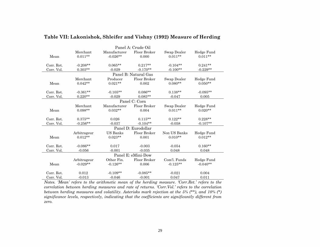
Table VII shows mean values for the herding measure. The mean values for each

commodity are fairly small, but statistically different from zero. For example, in the crude

oil market, the average herding for hedge funds is 1.1 percent, implying that 51.1 percent of

hedge funds increased positions while 48.9 percent decreased positions on the average day.

The largest average values for the herding measure are in the natural gas market for swap

dealers (8 percent), in the corn market for merchants (8.83 percent), and in the eMini-Dow

for other financial institutions (-12.6 percent) and commercial funds (-12.5 percent).19

Table VII also shows the daily correlations of herding with returns and volatility for

each of the five markets. Notably, we see that herding among hedge funds and swap dealers

is, when significant, negatively related to volatility, indicating that hedge fund and swap

dealer herding is mainly countercyclical. Interestingly, hedge fund and swap dealer herding

is positively linked to rate of returns (except for hedge funds in natural gas and swap

dealers in crude oil). These results suggest that the Granger-causality results we document

above stem more generally from hedge fund position changes and not from a dominant

hedge fund.

Contrary to herding among speculative groups, merchant and floor broker herding is

highly correlated with returns and volatility. In particular, herding among merchants is

negatively linked to rate of returns but positively linked to volatility in the crude oil and

natural gas markets. In these markets, however, the economic effect of merchant herding is

relatively small and given the fact that information arrival can lead to clustering of traders

on one side of the market (and hence, a higher herding measure), these correlations are

only suggestive. Herding among floor brokers is negatively correlated with volatility for the

crude oil and corn markets but positively correlated with returns in the crude oil, natural

gas and corn markets.

19 By comparison, Lakonishok et al. (1992) document herding of 2.7 percent among equity money managers. Boyd et al. (2010) examine herding in futures markets in more detail.

19

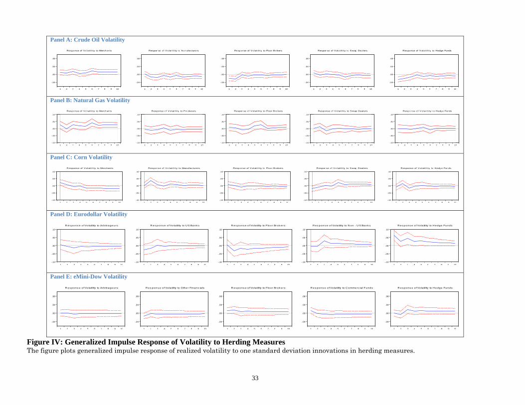
To investigate the effects of herding on returns and volatility, we run Granger-non-

causality tests (similar to those reported in Section IV) using herding as an alternative

measure of speculative activity. We find no significant link between returns and herding in

any of the five markets we analyze. However, Granger-causality results for volatility and

herding show a feed-back effect between volatility and herding measures for the crude oil,

corn and eMini-Dow markets.20 To further investigate this issue, we compute generalized

impulse responses and present results in Figure IV. A one standard deviation shock to

hedge fund herding has almost no significant effect on volatility, except in crude oil where

herding among hedge funds serves to reduce volatility levels (Panel A). Interestingly, an

unexpected shock to herding among hedge funds increases volatility levels in the

Eurodollar market. Swap dealer herding does not impact volatility, while a shock to

merchant herding increases volatility levels only in the natural gas and corn markets.

VII. Conclusion We employ a unique dataset that allows us to precisely identify positions of market

participants in five actively-traded and recently volatile futures markets to investigate

whether speculation moves prices and/or increases market volatility. Through correlations,

Granger-causality tests, and contemporaneous tests with instrumental variables, we find

that speculative groups like hedge fund and commodity swap dealer position changes do not

lead price changes, but rather lead to reduced market volatility. As a whole, these

speculative traders provide liquidity and do not destabilize futures markets.

Importantly, these results hold uniformly across a variety of financial and

commodity futures products over recent periods when turmoil in financial markets has

generated historically high levels of volatility. Indeed our results hold both for periods when

prices trend upward and also for periods where prices drop significantly and market

volatility spikes. Our results are also robust to measuring speculation by the total net

positions taken by hedge funds and swap dealers and by herding among hedge funds and to

various alternative volatility metrics.

These results are consistent Deuskar and Johnson’s (2010) conjecture that investors

with constant risk tolerance (like hedge funds perhaps) can trade profitably against flow-

driven shocks. Indeed, the increased positions taken in recent years by hedge funds and

20 For herding, we are unable to identify a valid instrument to replicate results from Section V.

20

swap dealers across a wide variety of futures markets may simply reflect a rational profit

motive. These speculative groups have not been destabilizing markets, but rather have

served to dampen volatility during the recent financial crisis.

Although we do not rule out the possibility that traders might attempt to (or

actually succeed to) move prices and increase volatility over short intervals of time, we find

no systematic, deleterious link between the trades of hedge funds or swap dealers and

either returns or volatility. Hedge fund trading, in fact, is commonly related to returns and

volatility, but in a beneficial sense—hedge funds commonly provide liquidity in futures

markets, reducing market volatility. In general, speculators like hedge funds and swap

dealers should not be viewed by hedgers as adversarial agents. Rather, speculative trading

activity serves to reduce market volatility and provides the necessary liquidity for the

proper functioning of financial markets.

21

References

Andersen, Torben, Tim Bollerslev, Francis X. Diebold, and Heiko Ebens. 2001. “The Distribution of Realized Stock Return Volatility.” Journal of Financial Economics 61 (July): 43-76.

Andersen, Torben, Tim Bollerslev, Francis X. Diebold, and Paul Labys. 2000. “Great

Realizations.” Risk 13 (March): 105-108. Andersen, Torben, Tim Bollerslev, Francis X. Diebold, and Paul Labys. 2003. “Modeling and

Forecasting Realized Volatility.” Econometrica 71 (March): 579-625. Barndorff-Nielsen, Ole E., Peter R. Hansen, Asger Lunde, and Neil Shephard. 2008.

“Designing Realized Kernels to Measure the ex post Variation of Equity Prices in the Presence of Noise.” Econometrica 76 (November): 1481-1536.

Boyd, Naomi, Bahattin Büyükşahin, Michael S. Haigh, and Jeffrey H. Harris. 2010. “The

Prevalence, Sources and Effects of Herding in Futures Markets.” Working paper, Commodity Futures Trading Commission.

Brown, Steven J., William N. Goetzmann, and James M. Park. 2000. “Hedge Funds and the

Asian Currency Crisis of 1997.” Journal of Portfolio Management 26 (Summer): 95-101. Brunnermeier, Markus K., and Stefan Nagel. 2004. “Hedge Funds and the Technology

Bubble.” Journal of Finance 59 (October): 2013-2040. Büyükşahin, Bahattin, Michael S. Haigh, Jeffrey H. Harris, Michel Robe, and James

Overdahl. 2010. “Fundamentals, Trading Activity and Derivative Pricing.” Working paper, Commodity Futures Trading Commission.

Büyükşahin, Bahattin, and Jeffrey H. Harris. 2010. Do Speculators Drive Crude Oil

Futures Prices? Energy Journal. Forthcoming. De Long, J. Bradford, Andrei Shleifer, Lawrence H. Summers, and Robert J. Waldmann.

1990. “Noise Trader Risk in Financial Markets.” Journal of Political Economy 98 (August): 704-738.

Deuskar, Prachi, and Timothy C. Johnson. 2010. "Market Liquidity and Flow-Driven Risk."

University of Illinois at Urbana-Champaign Working Paper. Edwards, Franklin R. 1999. “Hedge Funds and the Collapse of Long Term Capital

Management,” Journal of Economic Perspectives 13 (Winter): 189-210. Friedman, Milton. 1953. “The Case for Flexible Exchange Rates.” In Essays in Positive

Economics, University of Chicago Press, Chicago, 157-203. Fung, William, and David A. Hsieh. 2000. “Measuring the Market Impact of Hedge Funds.”

Journal of Empirical Finance, 7 (May): 1-36.

22

Griffin, John M., Jeffrey H. Harris, Tao Shu and Selim Topaloglu, 2010, “Who Drove and

Burst the Tech Bubble?,” Working Paper. Hasbrouck, Joel. 2003. “Intraday Price Formation in U.S. Equity Index Markets.”Journal of

Finance 58 (December): 2375-2400. Hirshleifer, David A. 1989. “Determinants of Hedging and Risk Premia in Commodity

Futures Markets.” Journal of Financial and Quantitative Analysis 24 (September): 313-331.

Hirshleifer, David A. 1990. “Hedging Pressure and Futures Price Movements in a General

Equilibrium Model.” Econometrica 58 (March): 411-428. Keynes, John M. 1923. “Some Aspects of Commodity Markets.” Manchester Guardian

Commercial, Reconstruction Supplement, in The Collected Writings of John Maynard Keynes, Vol. 12. London: Macmillan.

Lakonishok, Josef., Andrei. Shleifer and Robert W. Vishny. 1992. The impact of institutional trading on stock prices. Journal of Financial Economics 32, 23–43. Lux, Thomas. 1995. “Herd Behaviour, Bubbles and Crashes.” The Economic Journal 105

(July): 881-896 Pesaran, H. Hashem, and Yongcheol Shin. 1998. “Generalized Impulse Response Analysis

in Linear Multivariate Models.” Economics Letters 58 (January): 17-29. Shiller, Robert J. 2003. “From Efficient Markets Theory to Behavioral Finance.” Journal of

Economic Perspectives 17 (Winter): 83-104. Shleifer, Andrei and Lawrence H. Summers. 1990. “The Noise Trader Approach to

Finance.” The Journal of Economic Perspectives 4 (Spring): 19-33. Stock, James H., and Motohiro Yogo. 2005. Testing for Weak Instruments in Linear IV

Regression, in D.W.K. Andrews and J.H. Stock, eds., Identification and Inference for Econometric Models: Essays in Honor of Thomas Rothenberg, Cambridge: Cambridge University Press, 80–108.

Zhang, Lan, Per A. Mykland, and Yacine Aït-Sahalia. 2005. “A Tale of Two Time Scales:

Determining Integrated Volatility with Noisy High Frequency Data.” Journal of the American Statistical Association 100 (December): 1394-1411.

23

Table I: Descriptive Statistics

Panel A: Crude Oil – January 2005-March 2009 – 1047 obs. Returns Volatility Merchant Manufacturer Floor Broker Swap Dealer Hedge Fund

Mean -0.046 3.803 -64.21 512.7 146.62 -159.69 -1285 Median 0.059 2.171 306.0 272.0 18 -492 -1295 Std.Dev. 2.514 4.556 6783 3162 2228.9 8207.6 6644

Panel B: Natural Gas – January 2005-March 2009 – 1053 obs. Returns Volatility Merchant Producer Floor Broker Swap Dealer Hedge Fund

Mean -0.188 5.278 89.89 6.549 64.73 -381.8 -70.39 Median -0.157 3.927 26.00 0.000 39.00 -510.0 -246.0 Std.Dev. 3.056 4.465 1429 428.4 1442 2867 3423

Panel C: Corn – August 2006-March 2009 – 646 obs. Returns Volatility Merchant Manufacturer Floor Broker Swap Dealer Hedge Fund

Mean 0.025 3.153 868.2 -116.6 -208.0 -328.7 -362.8 Median 0.000 2.535 830.5 -152.5 -151.5 -620.0 -423.3 Std.Dev. 2.303 2.306 6669 1400 4191 7937 6918

Panel D: Eurodollar – January 2005-May 2008 – 1045 obs. Returns Volatility Arbitrageur US Banks Floor Broker Non US Banks Hedge Fund

Mean 0.000 0.003 -555.1 476.9 933.4 202.3 -35.45 Median 0.000 0.001 16.00 443.0 686.0 115.0 -1148 Std.Dev. 0.059 0.005 15625 13035 14571 12341 25395

Panel E: Mini-Dow – January 2005-May 2008 – 1038 obs. Returns Volatility Arbitrageur Other Fin’l. Floor Broker Com'l. Funds Hedge Fund

Mean -0.044 1.303 116.7 12.16 15.66 -77.66 -45.63 Median 0.043 0.363 222.0 10.00 -65.50 -3.000 -28.00 Std.Dev. 1.442 3.189 2912 547.1 1972 1750 2707

Notes. Volatility refers to the two-scale realized volatility estimator of Zhang et al.(2005). Trader positions refer to net (futures long minus futures short) daily changes.

24

Table II: Long/Short Percentage of Total Open Interest

Panel A: Crude Oil Total Merchant Manufacturer Floor

Broker Swap Dealer

Hedge Funds

Mean Max Min

Long 0.074 0.010 0.021 0.417 0.233 0.754 0.878 0.524 Short 0.296 0.102 0.048 0.064 0.224 0.734 0.849 0.576

Panel B: Natural Gas Total Merchant Producer Floor

Broker Swap Dealer

Hedge Funds

Mean Max Min

Long 0.074 0.008 0.024 0.385 0.286 0.777 0.912 0.623 Short 0.159 0.027 0.046 0.069 0.567 0.868 0.999 0.686

Panel C: Corn Total Merchant Manufacturer Floor

Broker Swap Dealer

Hedge Funds

Mean Max Min

Long 0.053 0.034 0.058 0.413 0.198 0.756 0.847 0.611 Short 0.437 0.048 0.087 0.016 0.159 0.746 0.845 0.634

Panel D: Eurodollar Total Arbitrageur US Bank Floor

Broker Non-US

Bank Hedge Fund

Mean Max Min

Long 0.143 0.037 0.043 0.088 0.125 0.435 0.680 0.211 Short 0.241 0.073 0.020 0.127 0.122 0.584 0.798 0.391

Panel E: eMini-Dow Total Arbitrageur Other Fin’l Floor

Broker Com’l Fund

Hedge Fund

Mean Max Min

Long 0.295 0.015 0.107 0.163 0.098 0.677 0.873 0.346 Short 0.280 0.028 0.149 0.059 0.082 0.599 0.803 0.274

Notes. Total Mean, Max, Min refers to mean, maximum and minimum, respectively, of the sum of the open interest of the five categories of market participants in each market. It indicates the percentage of total open interest jointly held by these five categories of traders.

25

Table III: Correlations – Net Futures Positions

Panel A: Crude Oil Merchant Manufacturer Floor Broker Swap Dealer Hedge Fund Returns -0.061* -0.139** -0.082** 0.051 0.319** Volatility -0.032 -0.051 0.021 0.062* -0.031 Manufacturer 0.251** 1 Floor Broker 0.023 0.038 1 Swap Dealer -0.644** -0.411** -0.182** 1 Hedge Fund -0.231** -0.232** -0.119** -0.252** 1

Panel B: Natural Gas Merchant Producer Floor Broker Swap Dealer Hedge Fund Returns -0.184** -0.199** -0.231** 0.019 0.181** Volatility 0.074** 0.052 0.008 -0.062* 0.022 Producer 0.092** 1 Floor Broker 0.143** 0.051 1 Swap Dealer -0.341** -0.173** -0.181** 1 Hedge Fund -0.082** -0.081** -0.301** -0.621** 1

Panel C: Corn Merchant Manufacturer Floor Broker Swap Dealer Hedge Fund Returns -0.372** -0.289** 0.052 0.002 0.451** Volatility 0.011 -0.051 0.081* -0.071 -0.011 Manufacturer 0.342** 1 Floor Broker 0.052 0.023 1 Swap Dealer -0.543** -0.229** -0.459** 1 Hedge Fund -0.512** -0.311** -0.091** -0.129** 1

Panel D: Eurodollar Arbitrageurs US Bank Floor Broker Non-US Bank Hedge Fund Returns -0.202** 0.041 0.011 -0.073** 0.192** Volatility -0.042 0.009 -0.017 0.01 -0.026 US Bank -0.082** 1 Floor Broker -0.024 -0.061* 1 Non-US Bank -0.073** -0.013 0.122** 1 Hedge Fund -0.331** -0.219** 0.131** -0.091** 1

Panel E: eMini-Dow Arbitrageur Other Fin’l. Floor Broker Com'l. Funds Hedge Fund Returns 0.13** -0.301** -0.104** 0.001 0.212** Volatility -0.01 -0.011 -0.031 0.019 0.003 Other Financial -0.09** 1 Floor Broker -0.06* 0.029 1 Com’l. Funds -0.12** 0.021 -0.481** 1 Hedge fund -0.50** -0.253** -0.227** 0.003 1 Notes. Asterisks mark rejection at the 5%(**) and 10% (*) significance levels, respectively, indicating that the correlation coefficients are significantly different from zero.

26

Table IV: Granger non-Causality Test: Returns and Changes in Net Futures Positions Panel A: Crude Oil – Optimal Lag-Length (5)

Returns Merchant Manufacturer Floor Broker Swap Dealer Hedge Fund All

Returns 0.253 0.211 0.218 0.362 0.533 0.199

Merchant 0.000** 0.317 0.420 0.011** 0.016** 0.000**

Manufacturer 0.000** 0.004** 0.052* 0.000** 0.003** 0.000**

Floor Broker 0.017** 0.353 0.416 0.011** 0.252 0.000**

Swap Dealer 0.001** 0.195 0.000** 0.217 0.590 0.000**

Hedge Fund 0.013** 0.427 0.433 0.380 0.030** 0.000**

Total 0.000** 0.001** 0.000** 0.067* 0.000** 0.086* Panel B: Natural Gas – Optimal Lag-Length (3)

Returns Merchant Producer Floor Broker Swap Dealer Hedge Fund All

Returns 0.448 0.403 0.345 0.503 0.666 0.571

Merchant 0.206 0.013** 0.913 0.009** 0.841 0.000**

Producer 0.124 0.301 0.908 0.000** 0.303 0.000**

Floor Broker 0.019** 0.106 0.001** 0.194 0.308 0.000**

Swap Dealer 0.000** 0.385 0.000** 0.502 0.535 0.000**

Hedge Fund 0.036** 0.025** 0.000** 0.889 0.652 0.000**

Total 0.000** 0.000** 0.000** 0.923 0.000** 0.240 Panel C: Corn – Optimal Lag-Length (5)

Returns Merchant Manufacturer Floor Broker Swap Dealer Hedge Fund All

Returns 0.285 0.777 0.823 0.799 0.394 0.442

Merchant 0.004** 0.388 0.591 0.544 0.892 0.002**

Manufacturer 0.633 0.745 0.899 0.910 0.861 0.960

Floor Broker 0.799 0.056* 0.001** 0.059 0.047* 0.000**

Swap Dealer 0.355 0.607 0.000** 0.352 0.948 0.000**

Hedge Fund 0.240 0.327 0.001** 0.957 0.101 0.000**

Total 0.101 0.018** 0.000** 0.483 0.563 0.158 Panel D: Eurodollar – Optimal Lag-Length (4)

Returns Arbitrageur US Bank Floor Broker Non-US Bank Hedge Fund All

Returns 0.174 0.203 0.165 0.226 0.315 0.478

Arbitrageur 0.380 0.727 0.051* 0.671 0.924 0.144

US Bank 0.254 0.511 0.139 0.861 0.27 0.196

Floor Broker 0.731 0.020** 0.173 0.439 0.228 0.239

Non-US Bank 0.381 0.897 0.001** 0.100 0.654 0.000**

Hedge Fund 0.548 0.005** 0.301 0.005** 0.594 0.001**

Total 0.495 0.000** 0.001** 0.004** 0.169 0.411 Panel E: eMini-Dow – Optimal Lag-Length (3)

Returns Arbitrageur Other Fin’l. Floor Broker Com'l. Fund Hedge Fund All

Returns 0.057* 0.010** 0.471 0.221 0.071 0.026**

Arbitrageur 0.097* 0.818 0.658 0.590 0.007** 0.000**

Other Fin’l. 0.165 0.261 0.171 0.518 0.191 0.232

Floor Broker 0.237 0.762 0.219 0.918 0.350 0.521

Com'l. Fund 0.07* 0.588 0.000** 0.434 0.283 0.000**

Hedge Fund 0.09* 0.102 0.444 0.250 0.332 0.004**

Total 0.038** 0.089* 0.000** 0.362 0.360 0.008** Notes. The table reports p-values of the Granger-causality test. Asterisks mark rejection at the 5% (**) and 10% (*) significance levels, respectively, indicating evidence of Granger causality.

27

Table V: Granger non-Causality Test: Volatility and Changes in Net Futures Positions Panel A: Crude Oil – Optimal Lag-Length (5)

Volatility Merchant Manufacture

r Floor Broker Swap Dealer Hedge Fund All

Volatility 0.066* 0.062* 0.025** 0.001** 0.072* 0.000**

Merchant 0.223 0.209 0.117 0.064* 0.000** 0.000**

Manufacturer 0.556 0.000** 0.023** 0.000** 0.000** 0.000**

Floor Broker 0.063 0.124 0.394 0.098* 0.596 0.000**

Swap Dealer 0.001** 0.185 0.000** 0.242 0.557 0.000**

Hedge Fund 0.079* 0.453 0.086* 0.284 0.028** 0.000**

Total 0.007** 0.000** 0.000** 0.001** 0.000** 0.000** Panel B: Natural Gas – Optimal Lag-Length (3)

Volatility Merchant Producer Floor Broker Swap Dealer Hedge Fund All

Volatility 0.974 0.476 0.066* 0.065* 0.667 0.052*

Merchant 0.951 0.001** 0.996 0.014** 0.865 0.000**

Producer 0.169 0.105 0.975 0.000** 0.244 0.000**

Floor Broker 0.477 0.154 0.001** 0.286 0.344 0.000**

Swap Dealer 0.391 0.538 0.000** 0.819 0.139 0.000**

Hedge Fund 0.044 0.015** 0.000** 0.976 0.354 0.000**

Total 0.344 0.002** 0.000** 0.879 0.000** 0.437 Panel C: Corn – Optimal Lag-Length (5)

Volatility Merchant Manufacturer Floor Broker Swap Dealer Hedge

Fund All

Volatility 0.711 0.892 0.174 0.266 0.330 0.020**

Merchant 0.034** 0.337 0.439 0.147 0.893 0.010**

Manufacturer 0.222 0.722 0.940 0.816 0.795 0.868

Floor Broker 0.011** 0.022* 0.000** 0.046** 0.045** 0.000**

Swap Dealer 0.431 0.774 0.000** 0.246 0.906 0.000**

Hedge Fund 0.839 0.168 0.001** 0.973 0.234 0.000**

Total 0.004** 0.013** 0.000** 0.500 0.158 0.148 Panel D: Eurodollar – Optimal Lag-Length (5)

Volatility Arbitrageu

r US Bank Floor Broker Non-US Bank Hedge Fund All

Volatility 0.053* 0.085* 0.058* 0.104 0.007** 0.025**

Arbitrageur 0.278 0.192 0.668 0.370 0.279 0.059*

US Bank 0.642 0.015** 0.285 0.754 0.211 0.373

Floor Broker 0.054* 0.573 0.147 0.592 0.047** 0.084*

Non-US Bank 0.575 0.153 0.021** 0.079* 0.001** 0.000**

Hedge Fund 0.111 0.846 0.196 0.002** 0.946 0.002**

Total 0.239 0.015** 0.001** 0.000** 0.198 0.000** Panel E: eMini-Dow– Optimal Lag-Length (4)

Volatility Arbitrageu

r Other Fin’l Floor Broker Com'l. Fund Hedge Fund All

Volatility 0.042** 0.162 0.909 0.270 0.043** 0.007**

Arbitrageur 0.741 0.799 0.651 0.153 0.008** 0.001**

Other Fin’l. 0.370 0.590 0.275 0.640 0.335 0.435

Floor Broker 0.016** 0.583 0.213 0.118 0.530 0.011**

Com'l. Fund 0.069* 0.138 0.000** 0.474 0.389 0.000**

Hedge Fund 0.359 0.134 0.770 0.325 0.348 0.043**

Total 0.110 0.089* 0.000** 0.617 0.010** 0.008** Notes. The table reports p-values of the Granger-causality test. Asterisks mark rejection at the 5% (**) and 10% (*) significance levels, respectively, indicating evidence of Granger causality.

28

Table VI: OLS and IV Estimates of Realized Volatility on Trader Positions Panel A: Crude Oil

Merchant Manufacturer Floor Broker Swap Dealer Hedge Fund OLS Coeff. 3.52e-4**

(9.22e-5) 2.11e-4

(1.99e-4) 6.24e-4** (2.19e-4)

-2.29e-4** (7.64e-5)

-2.44e-4 (9.33e-4)

R2 (%) 77.59 77.29 77.37 77.46 77.41

IV Coeff. 2.71e-4** (1.01e-4)

6.18e-5 (2.05e-4)

5.41e-4** (2.73e-4)

-1.20e-4 (9.17e-5)

-2.88e-4** (8.31e-5)

F-Stat 113.1 46.08 9.948 321.5 16.38

Panel B: Natural Gas Merchant Producer Floor Broker Swap Dealer Hedge Fund

OLS Coeff. 2.07e-3** (8.93e-4)

4.74e-4 (2.95e-4)

-1.91e-4 (8.17e-4)

-9.02e-4** (4.53e-4)

2.41e-4 (3.13e-4)

R2 (%) 32.75 32.39 32.39 32.65 32.42

IV Coeff. 1.76e-3* (9.73e-4)

-1.26e-4 (2.54e-3)

-2.94e-4 (7.63e-4)

-6.43e-4 (5.19e-4)

-8.29e-05** (3.60e-5)

F-Stat 34.40 17.72 8.6691 117.67 43.11

Panel C: Corn Merchant Manufacturer Floor Broker Swap Dealer Hedge Fund OLS Coeff. 5.44e-5

(1.51e-4) -4.50e-4 (7.12e-4)

3.38e-4 (2.50e-4)

-1.86e-4 (1.31e-4)

3.63e-5 (1.60e-4)

R2 (%) 45.74 45.76 45.89 45.91 45.73

IV Coeff. 1.37e-5 (1.66e-4)

-5.11e-4 (7.55e-4)

2.95e-4 (2.84e-4)

-1.45e-4 (1.72e-4)

-3.57e-5 (1.53e-4)

F-Stat 33.38 12.276 14.082 70.70 10.092

Panel D: Eurodollar Arbitrageur US Bank Floor Broker Non-US Bank Hedge Fund

OLS Coeff. -2.08e-4** (9.36e-5)

-1.82e-4 (1.12e-4)

5.22e-5 (1.00e-4)

1.18e-4 (1.18e-4)

2.12e-5 (5.78e-5)

R2 (%) 62.55 62.46 62.37 62.40 62.36

IV Coeff. 2.26e-4** (1.02e-4)

-1.76e-4 (1.31e-4)

5.86e-5 (7.45e-5)

1.17e-4 (1.07e-4)

2.51e-5 (6.23e-5)

F-Stat 1.6155 1.5651 15.827 3.4869 14.396

Panel E: eMini-Dow Arbitrageur Other Financial Floor Broker Com'l Fund Hedge Fund

OLS Coeff. -1.07e-3** (4.12e-4)

8.91e-3** (2.50e-3)

1.29e-3* (6.88e-4)

-3.66e-5 (7.83e-4)

-1.22e-4 (5.02e-4)

R2 (%) 86.45 86.56 86.43 86.38 86.44

IV Coeff. -1.10e-3* (5.76e-4)

8.92e-3** (2.73e-3)

1.30e-3* (7.98e-4)

-2.48e-5 (9.29e-4)

-1.42e-3** (4.86e-4)

F-Stat 21.111 18.735 5.8920 10.619 50.442 Notes. The tables reports OLS and Instrumental Variables estimates of the contemporaneous effect of trader position changes (in absolute value) on volatility. Asterisks mark rejection at the 5% (**), and 10% (*) significance levels, respectively, indicating that the coefficients are significantly different from zero. The F-statistics in excess of 8.96 indicates that the change in the number of reporting traders is a valid instrument.

29

Table VII: Lakonishok, Shleifer and Vishny (1992) Measure of Herding

Panel A: Crude Oil Merchant Manufacturer Floor Broker Swap Dealer Hedge Fund

Mean 0.011** -0.026** 0.000 0.011** 0.011**

Corr. Ret. -0.208** 0.065** 0.217** -0.104** 0.241** Corr. Vol. 0.303** -0.029 -0.170** -0.100** -0.229**

Panel B: Natural Gas Merchant Producer Floor Broker Swap Dealer Hedge Fund

Mean 0.042** 0.021** 0.002 0.080** 0.050**

Corr. Ret. -0.361** -0.105** 0.086** 0.138** -0.095** Corr. Vol. 0.220** -0.029 0.085** -0.047 0.005

Panel C: Corn Merchant Manufacturer Floor Broker Swap Dealer Hedge Fund

Mean 0.098** 0.032** 0.004 0.011** 0.020**

Corr. Ret. 0.375** 0.026 0.115** 0.122** 0.228** Corr. Vol. -0.256** -0.037 -0.104** -0.058 -0.107**

Panel D: Eurodollar Arbitrageur US Banks Floor Broker Non US Banks Hedge Fund

Mean 0.012** 0.023** 0.001 0.010** 0.012**

Corr. Ret. -0.086** 0.017 -0.003 -0.054 0.160** Corr. Vol. -0.056 -0.001 -0.035 0.048 0.048

Panel E: eMini-Dow Arbitrageur Other Fin. Floor Broker Com'l. Funds Hedge Fund

Mean -0.029** -0.126** 0.006 -0.125** -0.040**

Corr. Ret. 0.012 -0.109** -0.085** -0.021 0.004 Corr. Vol. -0.013 -0.046 -0.001 0.047 0.011

Notes. ‘Mean’ refers to the arithmetic mean of the herding measure. ‘Corr.Ret.’ refers to the correlation between herding measures and rate of returns. ‘Corr.Vol.’ refers to the correlation between herding measures and volatility. Asterisks mark rejection at the 5% (**), and 10% (*) significance levels, respectively, indicating that the coefficients are significantly different from zero.

30

Figure I: Price and Realized Volatility The figure plots prices and realized volatility over the sample period January 2005 – March 2009.

31

eMini-Dow Returns

Figure II: Impulse Response of Returns The figure plots generalized impulse responses of returns to one standard deviation innovations in trader position changes for the eMini-Dow futures market.

-.004

-.002

.000

.002

.004

1 2 3 4 5 6 7 8 9 10

R es pons e of R eturns to Arbitrageurs

-.004

-.002

.000

.002

.004

1 2 3 4 5 6 7 8 9 10

R es pons e o f R e turns to Other Financ ia ls

-.004

-.002

.000

.002

.004

1 2 3 4 5 6 7 8 9 10

Res pons e of returns to Floor Brok ers

-.004

-.002

.000

.002

.004

1 2 3 4 5 6 7 8 9 10

R es pons e o f R etu rns to C ommerc ial Funds

-.004

-.002

.000

.002

.004

1 2 3 4 5 6 7 8 9 10

R es pons e o f R eturns to H edge Funds

32

Panel A: Crude Oil Volatility

Panel B: Natural Gas Volatility

Panel C: Corn Volatility

Panel D: Eurodollar Volatility

Panel E: eMini-Dow Volatility

Figure III: Generalized Impulse Response of Volatility The figure plots generalized impulse response of realized volatility to one standard deviation innovations in trader position changes.

-.04

-.02

.00

.02

.04

1 2 3 4 5 6 7 8 9 10

R es pons e o f Vo la tility to Merc hants

-.04

-.02

.00

.02

.04

1 2 3 4 5 6 7 8 9 10

R es pons e o f Vo la tility to Manu fac tu rers

-.04

-.02

.00

.02

.04

1 2 3 4 5 6 7 8 9 10

R es pons e o f Vo la tility to Floor Brok ers

-.04

-.02

.00

.02

.04

1 2 3 4 5 6 7 8 9 10

R es pons e o f Vo la tility to Sw ap D ea le rs

-.04

-.02

.00

.02

.04

1 2 3 4 5 6 7 8 9 10

R es pons e o f Vo la tility to H edge Funds

-.10

-.05

.00

.05

.10

.15

.20

1 2 3 4 5 6 7 8 9 10

R es pons e o f Vo la tility to Merc hants

-.10

-.05

.00

.05

.10

.15

.20

1 2 3 4 5 6 7 8 9 10

R es pons e o f Vo la tility to Produc ers

-.10

-.05

.00

.05

.10

.15

.20

1 2 3 4 5 6 7 8 9 10

R es pons e o f Vo la tility to Floo r Brok ers

-.10

-.05

.00

.05

.10

.15

.20

1 2 3 4 5 6 7 8 9 10

R es pons e o f Vo la tility to Sw ap D ea lers

-.10

-.05

.00

.05

.10

.15

.20

1 2 3 4 5 6 7 8 9 10

R es pons e o f Vo la tility to H edge Funds

-.050

-.025

.000

.025

.050

.075

.100

1 2 3 4 5 6 7 8 9 10

R es pons e o f Vo la tility to Merc hants

-.050

-.025

.000

.025

.050

.075

.100

1 2 3 4 5 6 7 8 9 10

R es pons e o f Vola tility to Manufac tu re rs

-.050

-.025

.000

.025

.050

.075

.100

1 2 3 4 5 6 7 8 9 10

R es pons e o f Vo la tility to Floor Brok ers

-.050

-.025

.000

.025

.050

.075

.100

1 2 3 4 5 6 7 8 9 10

R es pons e o f Vo la tility to Sw ap D eale rs

-.050

-.025

.000

.025

.050

.075

.100

1 2 3 4 5 6 7 8 9 10

R es pons e o f Vo la tility to H edge Funds

-.10

-.05

.00

.05

.10

.15

.20

1 2 3 4 5 6 7 8 9 10

R es pons e o f Vo latility to Arb itrageurs

-.10

-.05

.00

.05

.10

.15

.20

1 2 3 4 5 6 7 8 9 10

R es pons e o f Vola tility to U S Bank s

-.10

-.05

.00

.05

.10

.15

.20

1 2 3 4 5 6 7 8 9 10

R es pons e o f Vo la tility to Floor Brok ers

-.10

-.05

.00

.05

.10

.15

.20

1 2 3 4 5 6 7 8 9 10

R es pons e o f Vo la tility to N on-U S Bank s

-.10

-.05

.00

.05

.10

.15

.20

1 2 3 4 5 6 7 8 9 10

R es pons e of Vo la tility to H edge Funds

-.050

-.025

.000

.025

.050

.075

.100

1 2 3 4 5 6 7 8 9 10

R es pons e o f Vo latility to Arb itrageurs

-.050

-.025

.000

.025

.050

.075

.100

1 2 3 4 5 6 7 8 9 10

R es pons e o f Vo la tility to Other Financ ia ls

-.050

-.025

.000

.025

.050

.075

.100

1 2 3 4 5 6 7 8 9 10

R es pons e o f Vo latility to Floor Brok ers

-.050

-.025

.000

.025

.050

.075

.100

1 2 3 4 5 6 7 8 9 10

R es pons e of Vo la tility to C ommerc ia l Funds

-.050

-.025

.000

.025

.050

.075

.100

1 2 3 4 5 6 7 8 9 10

R es pons e o f Vo la tility to H edge Funds

33

Panel A: Crude Oil Volatility

Panel B: Natural Gas Volatility

Panel C: Corn Volatility

Panel D: Eurodollar Volatility

Panel E: eMini-Dow Volatility

Figure IV: Generalized Impulse Response of Volatility to Herding Measures The figure plots generalized impulse response of realized volatility to one standard deviation innovations in herding measures.

-.04

.00

.04

.08

1 2 3 4 5 6 7 8 9 10

Response of Volati l i ty to Merchants

-.04

.00

.04

.08

1 2 3 4 5 6 7 8 9 10

Response of V olati l i ty to Manufacturers

-.04

.00

.04

.08

1 2 3 4 5 6 7 8 9 10

Response of Volati l i ty to Floor Bri kers

-.04

.00

.04

.08

1 2 3 4 5 6 7 8 9 10

Response of Volati l i ty to Swap Dealers

-.04

.00

.04

.08

1 2 3 4 5 6 7 8 9 10

Response of V olati l i ty to Hedge Funds

-.10

-.05

.00

.05

.10

1 2 3 4 5 6 7 8 9 10

Response of Volati l i ty to Merchants

-.10

-.05

.00

.05

.10

1 2 3 4 5 6 7 8 9 10

Response of Volati l i ty to Producers

-.10

-.05

.00

.05

.10

1 2 3 4 5 6 7 8 9 10

Response of Volati l i ty to Floor Brokers

-.10

-.05

.00

.05

.10

1 2 3 4 5 6 7 8 9 10

Response of Volati l i ty to Swap Dealers

-.10

-.05

.00

.05

.10

1 2 3 4 5 6 7 8 9 10

Response of V olati l i ty to Hedge Funds

-.10

-.05

.00

.05

.10

1 2 3 4 5 6 7 8 9 10

Response of Volati l i ty to Merchants

-.10

-.05

.00

.05

.10

1 2 3 4 5 6 7 8 9 10

Response of Volati l i ty to Manufacturers

-.10

-.05

.00

.05

.10

1 2 3 4 5 6 7 8 9 10

Response of Volati l i ty to Floor Brokers

-.10

-.05

.00

.05

.10

1 2 3 4 5 6 7 8 9 10

Response of Volati l i ty to Swap Dealers

-.10

-.05

.00

.05

.10

1 2 3 4 5 6 7 8 9 10

Response of Volati l i ty to Hedge Funds

-.10

-.05

.00

.05

.10

1 2 3 4 5 6 7 8 9 10

R es pons e o f Vo la tility to Arb itrageurs

-.10

-.05

.00

.05

.10

1 2 3 4 5 6 7 8 9 10

R es pons e o f Vo la tility to U S Bank s

-.10

-.05

.00

.05

.10

1 2 3 4 5 6 7 8 9 10

R es pons e o f Vo la tility to Floo r Brok ers

-.10

-.05

.00

.05

.10

1 2 3 4 5 6 7 8 9 10

R es pons e o f Vo la tility to N on - U S Bank s

-.10

-.05

.00

.05

.10

1 2 3 4 5 6 7 8 9 10

R es pons e o f Vo la tility to H edge Funds

-.04

.00

.04

.08

1 2 3 4 5 6 7 8 9 10

R es pons e o f Vo la tility to Arb itrageurs

-.04

.00

.04

.08

1 2 3 4 5 6 7 8 9 10

R es pons e o f Vo la tility to Othe r Financ ia ls

-.04

.00

.04

.08

1 2 3 4 5 6 7 8 9 10

R es pons e o f Vo la tility to Floo r Brok ers

-.04

.00

.04

.08

1 2 3 4 5 6 7 8 9 10

R es pons e o f Vo la tility to C ommerc ia l Funds

-.04

.00

.04

.08

1 2 3 4 5 6 7 8 9 10

R es pons e o f Vo la tility to H edge Funds

34

Appendix: Contract Specifications Crude Oil (CL) Natural Gas (NG) Corn (C) EuroDollars (ED) eMini-Dow (YM) Exchange NYMEX NYMEX CBOT CME CBOT Trading Unit 1000 US barrel 10,000 mmBtu 5000 bushels Eurodollar time

deposit having a principal value of 1 million with a 3-month maturity

1 mini-sized Dow futures

Trading Hours (EST): Open Outcry: Electronic

9:00 am-2:30pm 6:00pm-5:15pm

9:00am-2:30pm 6:00pm-5:15pm

10:30am-2:15pm 7:00pm-7am and 10:30am-2:15pm

8:20am-3pm 6:00pm-5:00pm

N/A 6:00pm-4:15pm, and 4:30pm-5:30pm

Trading months

Consecutive months in the current year and the next five years as well as June and December contracts are beyond sixth year

Consecutive months in the current year and the next twelve years

Dec, Mar, May, Jul and Sep

Mar, Jun, Sep, Dec, forty months in March quarterly cycle, and the four nearest serial contract months

Mar, Jun, Sep, Dec

Minimum Price Fluctuations

$0.01 per barrel ($10 per contract)

$0.01 per mmBtu ($10 per contract)

1/4 cent/bushel ($12.50/contract)

$12.50 per contract

($6.25 for nearest expiring contract)

Minimum price increment is one index point (equal to $5 per contract).

Settlement Type

Physical Physical Physical Cash Cash

Last Trading Day

Trading terminates at the close of business on the third business day prior to the 25th calendar day of the month preceding the delivery month.

Trading terminates three business days prior to the first calendar day of the delivery month.

The business day prior to the 15th calendar day of the contract month.

Futures trading shall terminate at 5:00a.m. (Chicago Time on the second London bank business day before the third Wednesday of the contract month.

Trading can occur up to 8:30 a.m. on the 3rd Friday of the contract month.

Daily average (max-min) number of contract traded

39,498 (182,330-837)

7,943 (61,860-302)

21,041* (96,391-942)

8,355 (33,641-725)

73,022* (321,700-1,110)

Notes. Asterisk indicates that electronic trading occurs only during times when open outcry is trading (9:30am – 4:00pm EST for eMini-Dow).