spectroscopic factors and strength distributions for the ...kawabata/pub/phd_ysd.pdf ·...
TRANSCRIPT

Spectroscopic factors and strength distributions for thedeeply bound orbitals in 40Ca measured with the(~p,2p)
reaction at 392 MeV
YASUDA Yusuke
2011
(Ver 0.9)


Abstract
Cross sections and analyzing powers for the40Ca(~p,2p) reaction were measured. The strength distri-
butions for the deep-hole states were obtained by a multipole decomposition analysis and a background
subtraction. The centroid energies and widths of the hole-state strengths were obtained as 29.6±0.6 and
48.4± 0.6 MeV for the 1p and 1s1/2-hole states, respectively. The obtained spectroscopic factors of the
hole states for the valence orbitals were larger than those from the (e, e′p) and (d,3He) reactions, and
those of the 1d3/2-, 1d5/2-, and 1s1/2-hole states were over 100% of the 2J + 1 values. The qualitative
and quantitative reproduction of the DWIA calculation was discussed for the hole states of the valence
orbitals. Taking the uncertainty of the DWIA calculation into the consideration,the spectroscopic fac-
tors were normalized by using the value for the 1d3/2 orbital from the (e, e′p) reaction and discussed.
The normalized spectroscopic factors for the deeply bound 1p and 1s1/2 orbitals were 49± 7% and
89± 9% of the sum-rule limits of independent-particle shell model, respectively. Aninfluence of the
nucleon-nucleon correlations on the spectroscopic factors is suggested.


Contents
1 Introduction 1
1.1 Nucleon-nucleon correlations in nuclei . . . . . . . . . . . . . . . . . . . . .. . . . . 1
1.2 Spectroscopic studies . . . . . . . . . . . . . . . . . . . . . . . . . . . . . . . . .. . 2
1.3 Quasi-free knockout (p,2p) reaction . . . . . . . . . . . . . . . . . . . . . . . . . . . 4
1.4 Purposes of this work . . . . . . . . . . . . . . . . . . . . . . . . . . . . . . . . .. . 7
2 Experiment 11
2.1 Kinematics . . . . . . . . . . . . . . . . . . . . . . . . . . . . . . . . . . . . . . . . 11
2.2 Experimental conditions . . . . . . . . . . . . . . . . . . . . . . . . . . . . . . . . .13
2.3 Experimental setup . . . . . . . . . . . . . . . . . . . . . . . . . . . . . . . . . . . .14
2.3.1 Beam transportation and target . . . . . . . . . . . . . . . . . . . . . . . . . .14
2.3.2 Dual spectrometer system . . . . . . . . . . . . . . . . . . . . . . . . . . . . 16
2.3.3 Focal-Plane detectors of GR and LAS . . . . . . . . . . . . . . . . . . . . . .17
2.3.4 MWPC for scattering angles . . . . . . . . . . . . . . . . . . . . . . . . . . . 20
2.3.5 Trigger and data acquisition system . . . . . . . . . . . . . . . . . . . . . . . 23
3 Data Reduction 29
3.1 Polarization of proton beam . . . . . . . . . . . . . . . . . . . . . . . . . . . . . .. . 29
3.2 Particle Identification . . . . . . . . . . . . . . . . . . . . . . . . . . . . . . . . . . .30
3.3 Subtraction of accidental coincidences . . . . . . . . . . . . . . . . . . . . .. . . . . 32
3.4 Track reconstruction of scattered particles . . . . . . . . . . . . . . . . . .. . . . . . 33
i

ii CONTENTS
3.4.1 Multi-wire drift chambers . . . . . . . . . . . . . . . . . . . . . . . . . . . . 33
3.4.2 Trajectory of a charged particle . . . . . . . . . . . . . . . . . . . . . . . . .35
3.4.3 Efficiency of the MWDC . . . . . . . . . . . . . . . . . . . . . . . . . . . . . 36
3.5 Multi-wire proportional chambers . . . . . . . . . . . . . . . . . . . . . . . . . .. . 37
3.6 Solid angles . . . . . . . . . . . . . . . . . . . . . . . . . . . . . . . . . . . . . . . . 38
3.7 Normalization due to the trigger efficiency of the scintillation detectors . . . . . . . . . 38
3.8 Separation energy of40Ca(p,2p)39K reaction . . . . . . . . . . . . . . . . . . . . . . 40
3.9 Cross sections and analyzing powers . . . . . . . . . . . . . . . . . . . . . .. . . . . 40
3.10 pp-scattering . . . . . . . . . . . . . . . . . . . . . . . . . . . . . . . . . . . . . . . 42
4 Analysis 43
4.1 Distorted wave impulse approximation calculation . . . . . . . . . . . . . . . . . . .. 43
4.2 Multipole decomposition analysis withAy data . . . . . . . . . . . . . . . . . . . . . 47
5 Result 49
5.1 Separation-energy spectra . . . . . . . . . . . . . . . . . . . . . . . . . . . .. . . . . 49
5.2 Results for discrete states . . . . . . . . . . . . . . . . . . . . . . . . . . . . . . .. . 55
5.3 Results of the deeply bound states . . . . . . . . . . . . . . . . . . . . . . . . . .. . 57
5.3.1 Strength distributions . . . . . . . . . . . . . . . . . . . . . . . . . . . . . . . 59
5.3.2 Background consideration . . . . . . . . . . . . . . . . . . . . . . . . . . . .59
6 Discussion 77
6.1 DWIA calculation . . . . . . . . . . . . . . . . . . . . . . . . . . . . . . . . . . . . . 77
6.2 Spectroscopic factors and strength distributions . . . . . . . . . . . . . . .. . . . . . 82
6.2.1 Comparison with experimental works . . . . . . . . . . . . . . . . . . . . . . 82
6.2.2 Comparison with theoretical works . . . . . . . . . . . . . . . . . . . . . . . 84
6.3 Perspectives . . . . . . . . . . . . . . . . . . . . . . . . . . . . . . . . . . . . . .. . 87
7 Summary 89

CONTENTS iii
Acknowledgments 91
A Phase space calculation 93
A.1 Introduction . . . . . . . . . . . . . . . . . . . . . . . . . . . . . . . . . . . . . . . .93
A.2 Phase space for four-particle final state . . . . . . . . . . . . . . . . . . .. . . . . . . 93
A.3 Phase space for two-particle final state . . . . . . . . . . . . . . . . . . . . .. . . . . 95
A.4 two-body kinematics . . . . . . . . . . . . . . . . . . . . . . . . . . . . . . . . . . . 96
A.5 supplement . . . . . . . . . . . . . . . . . . . . . . . . . . . . . . . . . . . . . . . . 97
B Numerical data tables 99

Chapter 1
Introduction
1.1 Nucleon-nucleon correlations in nuclei
A nucleus is a many body system that consists of protons and neutrons interacting strongly, and a
description of a nuclear system has been studied long. The independent-particle shell model (IPSM)
in the nuclear mean field describes various nuclear-structure phenomena. It well explains distinctive
features of nucleus like the existence of magic numbers or the spins and parities of nuclei. Although the
nuclear mean field is built on the basis of nucleon-nucleon (NN) two-body interaction, some features of
NN interaction are neglected. The difference between the mean field potential and the actual sum ofNN
interactions is known as the residual interaction orNN correlations, and the residual interaction andNN
correlations are needed to describe nuclear structure in detail and attract many researchers. The short-
range correlations, which are related to the strong repulsive core of theNN two-body interaction, are
the most importantNN correlations. It has been an interesting topic how the strong repulsive interaction
between nucleons works in nuclei. Recently, the spin-isospin and tensor correlations have also received
much attention because they play an important role in the binding of nucleons and affect the shell
structure in exotic nuclei [1, 2].
One of the important quantities indicating the influence of theNN correlations on the shell-model
picture is a spectroscopic factor. For a reaction that involves a nucleon ina nucleus, such as knockout
and pickup reactions, this factor indicates how many nucleons participate in the reaction channel, and
approximately shows how many nucleons are in the orbital in the nucleus. From a naive shell-model
picture, orbitals in nuclei are filled by nucleons up to 2J + 1; J is a total angular momentum of the
orbital. Therefore, the maximum value of the spectroscopic factor for the orbital with a total angular
momentumJ is 2J + 1. The factor is obtained by dividing the measured cross section by the theoretical
cross section calculated for one nucleon in the orbital. For example, in a knockout reaction, an injected
particle interacts with a nucleon in a nucleus and the nucleon is ejected from thenucleus. The residual
nucleus is expected to be a one-hole state because a nucleon is independently moving in the nucleus in
the view of the IPSM. The theoretical calculation is performed under this condition. When the nucleon
in the nucleus strongly correlates with another nucleon, the residual nucleus is any longer expected to
1

2 CHAPTER 1. INTRODUCTION
be one-hole state and the correlated nucleon often ejects from the nucleusat the same time. Therefore,
the existence ofNN correlated pairs makes the spectroscopic factor for the expected reaction channel
decrease. In practice, the quenched spectroscopic factors are reported, as mentioned in Section 1.2.
Several experiments were performed by knockout reaction to directly measure the correlated nu-
cleon pairs. When a nucleon in a correlated pair is knocked out, the other nucleon in the pair recoils.
Correlated nucleon pairs were measured under the back-to-back kinematical condition as evidence of
short-range correlations by the (e, e′pp) reaction at the Thomas Jefferson National Accelerator Facility
(JLab) [3, 4] and at NIKHEF [5] and by the (e, e′pn) reaction at Maintz [6, 7] and by the (p,2pn) reac-
tion at Brookhaven National Laboratory (BNL) [8, 9]. At JLab, Subedi et al. measured the12C(e, e′pn),12C(e, e′pp), and12C(e, e′p) reactions simultaneously, and they suggested from their result that the 80%
of the nucleons in the12C move as described within the shell model, and 18% of them are p–n correlated
pairs and the rest of 2% are p–p and n–n correlated pairs.
1.2 Spectroscopic studies
The spectroscopic factors for orbitals in nuclei have been measured to investigate the influence of theNN
correlations on the shell structure. Early spectroscopic studies were performed by (d, 3He) reaction for
proton (e.g. Ref. [10]). As the progress of electron accelerators, experiments for quasi-free knockout
reactions were actively performed. At the Nationaal Instituut voor Subatomaire Fysica, Amsterdam
(NIKHEF), high resolution studies of the (e, e′p) reaction were carried out for nuclei in the wide mass
range from2H to 209Bi, as reviewed by Dieperink and Witt Huberts [11].
From the results of high resolution (e, e′p) experiments at NIKHEF, Lapikaset al. reported the spec-
troscopic factors for the nucleon orbitals close to the Fermi surface in16O, 40Ca,48Ca,90Zr, and208Pb
decrease to 60%–70% of the simple IPSM limits (2J + 1) and compared those factors with predictions
from nuclear matter calculations that include short-range and tensor correlations [12]. Figure 1.1 from
Ref. [12] shows summed spectroscopic strength as a function of the missingenergy. A large reduction
is observed near the Fermi surface. This reduction of the spectroscopic factor cannot be described in
the IPSM and it is expected to be ascribed to the presence of correlations between the nucleons, coming
from the residual nuclear interactions.
In theoretical point of view, in the 1950s, Jastrow introduced the influence of the strong two-body re-
pulsive force in may-body system by introducing a correlation function [14]. The function is multiplied
on wave functions and goes to zero when nucleons are in a short distance. Subsequently, the enhance-
ment of high momentum components in nucleon momentum distribution due to theNN correlations
have been predicted by theoretical works [15, 16, 17, 18, 19].
The reduced spectroscopic strength observed by (e, e′p) experiments at NIKHEF was explained by
Benharet al. using a microscopic nuclear matter calculation with the correlated basis function(CBF)
theory including theNN correlations and surface effects [13], as illustrated in Fig. 1.1. Both theNN
correlations and the surface effects contribute to the reduction of the hole-state strength near the Fermi

1.2. SPECTROSCOPIC STUDIES 3
Figure 1.1: Summed spectroscopic strength observed for proton knockout from various orbitals in theclosed-shell nuclei16O, 40Ca, 48Ca, 90Zr, and 208Pb as a function of the mean excitation energy ofthe orbital relative to the Fermi energy (ǫF) The dashed curve represents the quasi-particle strengthcalculated for nuclear matter, the solid curve is derived from the nuclear matter curve by includingsurface effects calculated for208Pb [13]. This figure is taken from Ref. [12].
surface, and the hole-state strengths far below the Fermi surface, where the surface effects are not
important, were suggested to decrease to almost 80% of the IPSM limits [13].
The other theoretical calculations performed with state-dependent correlations also suggested the
reduction of spectroscopic factors for deeply bound orbitals. The spectroscopic factors calculated by
Fabrociniet al. for the 1s and 1p orbitals are quenched to 70% and 90% of the IPSM limits in16O,
and to 55% and 58% in40Ca, respectively [20]. According to this calculation, the depletion of the
spectroscopic factors by theNN correlations is 10%–15% for the valence orbitals and 30%–45% for the
deeply bound orbitals. Most of the depletion was caused by the spin-isospin and tensor components of
the NN correlations. Biscontiet al. developed the calculation following Ref. [20] by Fabrociniet al.,
and predicted the spectroscopic factors for several doubly-closed-shell nuclei to be 80% or less of the
IPSM limit for the 1s and 1p orbitals in medium and heavy nuclei [21]. The spectroscopic factor for the
deepest 1s1/2 orbital is suppressed owing to theNN correlations most strongly of all the orbitals in both
of the calculations [20, 21].
Since the 1s1/2 orbital is the deepest bound orbital far below the Fermi surface, except for the very
light nuclei, the spectroscopic factor for the 1s1/2 orbital will not be affected by surface effects but will
be predominantly affected by theNN correlations. In medium and heavy nuclei, the 1p orbital is also far
below the Fermi surface and will be under the similar condition to that of the 1s1/2 orbital. Therefore,
it is interesting for the study ofNN correlations to investigate the spectroscopic factors for the deeply
4 CHAPTER 1. INTRODUCTION
bound orbitals in medium and heavy nuclei.
40Ca is a doubly magic nucleus in the medium-mass region. As40Ca has a core of closed shells
with 16 nucleons ( 8 protons and 8 neutrons), the 1s and 1p-orbitals in the inner core are suitable to
study correlations far below the Fermi surface. Many pioneering attempts were performed to examine
the single-particle behavior of the deep-hole states by the (e, e′p) [22, 23, 24, 25] and (p,2p) [26, 27]
reactions. Since deep-hole states in40Ca have large widths and overlap with adjacent hole states, the
strengths for the deep-hole states were determined by fitting the measured recoil-momentum distribution
of the cross section at each separation energy bin with the superposition of the knockout cross sections
for a few orbitals calculated within the distorted-wave impulse approximation (DWIA) [22, 23, 24, 26,
27]. Mougeyet al. presented spectroscopic factors of 75% of the IPSM limit for the 1s1/2 orbital and
95% for the 1p orbital [22]. Nakamuraet al. reported spectroscopic factors for the 1s1/2 and 1p orbitals
that are larger than the sum-rule limits [24]. Kullanderet al. also obtained much larger spectroscopic
factors [27]. The large spectroscopic factors in Refs. [24] and [27] are possibly caused by the small
theoretical cross sections and contamination from other processes. Thus, the reported spectroscopic
factors for the 1s1/2 and 1p orbitals in40Ca are not consistent among the previous experiments, and
these values of interest are still controversial.
1.3 Quasi-free knockout (p, 2p) reaction
Quasi-free scattering is one of the most direct methods to investigate the single-particle properties of
a nucleus such as spectroscopic factors or nucleon-momentum distributions and effects on the bound
nucleons of their environment in the nucleus. This is a process where an incident particle knocks a
nucleon out of a nucleus, which remains in a one-hole state. If the energyof the incoming particle and
the momentum transfer to the nucleon in the nucleus are sufficiently large, the influence of the other
spectator nucleons in the nucleus on the knock-out process can be neglected and the scattering of the
incident particle and the knocked-out nucleon is comparable with the scattering in a free space. This is
why the process is called quasi-free or quasi-elastic scattering. As quasi-free knockout reactions have
three-body final states, measurements can be made at various kinematical conditions to investigate a
momentum distribution of a nucleon in nuclei.
The first experiments of such processes were the (p,2p) reaction experiments, which were performed
at Berkeley with 340 MeV incident proton beam for light nucleus targets and the coincident proton
pairs were observed [28, 29]. Subsequently, the (p,2p) reaction experiments have been performed with
medium-energy proton beams at Uppsala, CERN, Liverpool, and so on, as reviewed in Ref. [30, 31, 32].
For the description of the (p,2p) reaction, DWIA calculation has been used and developed. According
to the impulse approximation, the proton-proton matrix element is directly expressed in terms of an
experimental quantity, that is, free proton-proton cross section for the kinematics of the experiment. The
three wave functions of the incoming and outgoing protons are distorted by complex optical potentials.
The distortion smears out the shapes of the angular correlations that are expected from the momentum
distributions in the orbitals and reduces the intensity. This reduction reflects inelastic multiple scattering
1.3. QUASI-FREE KNOCKOUT (P,2P) REACTION 5
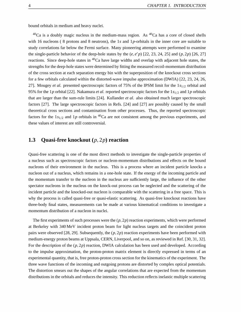
Figure 1.2: Analyzing powers for the 1p3/2 and p1/2-hole states for16O(p,2p) reaction measured bychanging a kinetic energy of an ejected proton. They behave differently as predicted by Jacob and Marisand show the validity of Maris effect. This figure is taken from Ref. [35]
that is another process than the quasi-free scattering. The intensity reduction due to multiple collisions
is severe for the (p,2p) reaction and reaches about 90% for heavy nuclei.
In the measurement of the (p,2p) reaction with a polarized proton beam, cross sections of the (p,2p)
reaction have asymmetries depending on the direction of the proton spin. In 1973, Jacob and Maris
suggested that the absorption in quasi-free scattering provides asymmetries of cross sections and for
the polarized proton beam asymmetries of cross sections for the hole states of the j> and j< orbitals
are expected to behave differently due to the spin–orbit coupling in the nucleus [33]. The asymmetries
of cross sections were measured with polarized proton beam at TRIUMF for 16O and40Ca at 200 MeV
[34, 35, 36] and for16O at 500 MeV [37], and theJ dependence of the asymmetries were experimentally
confirmed [32].
The analyzing powers for the 1p3/2 andp1/2-hole states for16O(p,2p) reaction measured by changing
a kinetic energy of an ejected proton are shown in Fig. 1.2 from Ref. [35]. They have different total
angular momenta and behave differently by changing an energy of ejected proton. This effect for the
asymmetry is called Maris effect. As a result of the longtime investigation of the (p,2p) reaction, the
asymmetry of the cross section for a hole state is recognized to be due to the spin–orbit part of the
optical potential for an orbital withL = 0 and to both the spin–orbit part and the effective polarization
(Maris effect) for aL , 0 orbital. TheAy data can provide the information on thej> and j< orbitals and
may separate their contributions in the cross sections.
Since the 1980s, the spectroscopic study by the (p,2p) reaction principally progressed at Indiana,
TRIUMF, Maryland, and iThemba [39, 35, 36, 37, 40, 41, 42, 43, 44]. The experiments were mostly
performed at the energy range of 100–200 MeV. The spectroscopic factors obtained with the DWIA
calculation were often different between the measurement conditions, that is, the absolute values of

6 CHAPTER 1. INTRODUCTION
Figure 1.3: Separation energies, widths, and angular momentum assignmentsof the hole states obtainedfrom quasi-free scattering, as functions of the atomic number. This figureis taken from Ref. [38]
the cross section from the DWIA calculation have some uncertainties. Nevertheless, iThemba group
obtained the spectroscopic factors for the hole states of the valence orbitals in 208Pb and found that they
are in good agreement with (e, e′p) studies [44].
The qualitative agreement on the asymmetry of the cross section between the DWIA calculation
and the measurement is not always satisfied. Although the DWIA calculation well reproduced the
asymmetries of the cross sections for the measurement with symmetric angle settings, it has problems on
the asymmetry forL , 0 orbitals for the measurement with asymmetric angle settings [32]. Moreover,
the asymmetries forL = 0 orbitals were not reproduced by the DWIA calculation quantitatively well;
the calculations overestimated the measurements. The influence of the environment in the nucleus on
theNN interaction has been discussed as the origin of the overestimation of the asymmetry [45, 46, 47,
48, 49].
Quasi-free (e, e′p) reaction measurement has also been performed since the 1960s [30, 31, 50, 51].
The intensity reduction and strong distortion are less severe in the (e, e′p) scattering because only the
outgoing proton suffers distortion from the optical potential. The cross sections are smaller than those of
the (p,2p) reaction due to the electromagnetic interaction between the incident electron and a nucleon
in a nucleus. The spectroscopic study by the (e, e′p) reaction were mainly performed for the hole states
of the valence orbitals in nuclei and provided spectroscopic factors with small uncertainties [52]. Since
the (e, e′p) reaction is recognized to be sensitive to whole of the bound-state wave function with respect
to the radial range [52], this reaction is necessary for the study of bound-state wave functions.

1.4. PURPOSES OF THIS WORK 7
Separation energies and widths for hole states were obtained from quasi-free reactions for the wide
mass-number range of nuclei, which directly revealed the existence of notonly surface but also inner
orbital shells in nuclei. Figure 1.3. from Ref. [38] is a famous figure on separation energies and widths
compiled by Jacob and Maris. For the heavier nuclei, the experimental knowledge for deeply bound
states was rather poor and has hardly been updated. Since the hole statesknocked out from the deep
orbital states are thought to have short lifetimes and large widths and they overlap each other, it is
difficult to identify deep hole states.
In the 1990s, the Petersburg Nuclear Physics Institute (PNPI) group reported that they had succeeded
in identifying the 1s1/2-hole states for medium- and heavy-mass nuclei such as40Ca, 90Zr, and208Pb
in the separation-energy spectra of (p,2p) and (p, np) reactions with a proton beam at 1 GeV [53, 54].
Figure 1.4 from Ref. [53] shows separation-energy spectra of (p,2p) (upper three figures in Fig. 1.4)
and (p, pn) (lower three figures in Fig. 1.4) reactions for40Ca target, and peaks of deepest 1s-hole states
are indicated. There is no other example identifying 1s-hole states in separation energy spectra for the
medium- and heavy-mass nuclei except PNPI group. The high energy 1 GeV injection beam might be
advantageous to identify deep hole states. Since the absolute cross sections were not measured, the
spectroscopic factors could not be given. However, these reports encouraged many researchers to study
deep-hole states again.
In 1999 and 2000, we performed (p,2p) experiments with 1 GeV proton beam at PNPI to identify
the hump of the 1s-hole state of40Ca in a separation energy spectrum and to measure its absolute
cross section simultaneously [55]. However, the 1s-hole state could not be identified in the separation
energy spectrum at that time. There was not a hump at expected separation energy region. The magnetic
spectrometers were set at an asymmetric angle condition and the measured kinetic energies of the ejected
two protons were unbalanced, following a previous work by Volkovet al [53]. Volkov et al. used
a magnetic spectrometer and a time of flight detector array that consists of scintillation counters to
analyze momenta of two protons, whereas, we used two magnetic spectrometers. The time of flight
detector array had 10 times smaller acceptance of the vertical angle than thatof a magnetic spectrometer.
A large detected vertical angle possibly accepted wide recoil momentum ranges of residual nuclei and
smeared the separation-energy spectrum.
1.4 Purposes of this work
The spectroscopic factors for deeply bound orbitals far below the Fermisurface are interesting quantities
to investigate the influence ofNN correlations on the single-particle states of nucleons. The purpose of
this work is to deduce the spectroscopic factors for deeply bound orbitalsand to discuss quenching of
the spectroscopic factors far below the Fermi surface.
For this purpose, we performed40Ca(p,2p) reaction experiment with a polarized proton beam at
392 MeV and measured the cross sections and analyzing powers. Although the intensity reduction for
the (p,2p) reaction due to multiple collisions is more severe than that for the (e, e′p) reaction, the

8 CHAPTER 1. INTRODUCTION
Figure 1.4: Separation-energy spectra for40Ca(p,2p) (upper three figures ) and40Ca(p, pn) (lower threefigures ) reactions measured with a 1 GeV proton beam at Petersburg Nuclear Physics Institute (PNPI)from Ref. [53]. The detection range of proton energy is (a) 830–870, (b) 855–887, and (c) 880–915 MeV.
(p,2p) reaction has an advantage to gain yields sufficiently for deep-hole states. Furthermore, theJ
dependence of the asymmetry of cross section of the (p,2p) reaction is also useful for identifying the
hole states when a polarized proton beam is used.40Ca is a suitable nucleus to study deeply bound
orbitals since40Ca is a nucleus in the medium-mass region and has a core of closed shells. It would be
premature to use much heavier nucleus than40Ca. The energy of 392 MeV of the injection proton is
higher than the energy of 200 MeV, where (p,2p) experiments were actively performed. Since both of
the ejected protons have larger kinetic energies than protons in case of 200 MeV injection, the protons
suffer less multiple collisions.
Identification of deep-hole states was an important step toward deducing thespectroscopic factors. At
the Research Center for Nuclear Physics (RCNP), Osaka University,the identification of 1s-hole state
in medium-mass nucleus, such as40Ca, had not been succeeded because it could not be found as a hump
in separation energy spectra. The separation of the contribution of deep-hole states by means of the
recoil-momentum distributions of the cross sections were performed in this work for the first time for
the data measured at RCNP. The identification of deep-hole states is essential for not only spectroscopic
study but also study on asymmetry of the (p,2p) cross section to investigate the influence of the nuclear
environment on theNN interaction. It is necessary to establish separation and identification of deep-hole
states in the (p,2p) reaction.
The reproduction of the cross section and analyzing power by the DWIA calculation has to be verified
at 392 MeV qualitatively and quantitatively. Though the DWIA calculation code used in this work
was mainly developed and applied to experiments around 200 MeV, the calculation has quantitative

1.4. PURPOSES OF THIS WORK 9
uncertainties in the absolute values of cross section even at this energy region. The previous (p,2p)
experiments at RCNP [46, 47, 48] were performed to investigate asymmetriesand the absolute values
of the cross sections were not discussed.
By use ofAy data, we planned to separatej> and j< hole states. The recoil-momentum distributions
of the analyzing power are distinctive for different total angular momentaJ of the orbitals even if
the corresponding orbital angular momentaL are the same. Therefore, the hole states induced from
the orbitals with the total angular momentaj> and j< can be distinguished in principle by use of the
analyzing power data. Separating 1p1/2- and 1p3/2-hole states is significant because 1p1/2- and 1p3/2-
hole states have not reasonably been separated in medium- or heavy-massnuclei yet.

10 CHAPTER 1. INTRODUCTION

Chapter 2
Experiment
The experiment was performed under Program No. E168 and E217 in thering cyclotron facility at
RCNP, Osaka University, with a 392-MeV polarized proton beam and the dual-arm spectrometer system
in the WS beam line. A schematic layout of the RCNP cyclotron facility is shown in Fig. 2.1.
2.1 Kinematics
In the (p,2p) reaction measurement, an injected proton interacts with a bound proton in the target
nucleus and both of the bound and injected protons go out from the nucleus. The knocked-out proton
and the scattered proton are measured in the experiment.
In the A(p,2p)B reaction with a target nucleusA and a residual nucleusB, as illustrated in Fig. 2.2,
the separation energyEsep is given by
Esep= T0 − T1 − T2 − T3 = Ex − Q, (2.1)
whereTi (i = 0,1,2,3) are the kinetic energies of the incident proton (i = 0), the scattered and knocked-
out protons (i = 1,2), and the residual nucleus (i = 3). The quantitiesEx andQ indicate the excitation
energy of the residual nucleusB and the reactionQ-value [ Q = MA − (MB + mp) ], respectively;MA,
MB, andmp are the masses of the target nucleus, the residual nucleus, and the proton. The separation
energy is the energy required to knock out a proton from a target nucleus, corresponding to the binding
energy of the knocked-out proton.
The momenta and the scattering angles of the two ejected protons were measured in the (p,2p)
measurement. Although the residual nucleus was not detected, its momentum (p3) was calculated from
the momenta of the incident proton and two ejected protons on the basis of the momentum conservation
law. Though the residual nucleus is a spectator for quasi-free knockout reactions in the view of the
IPSM, it recoils and has a momentum owing to the momentum conservation. The momentum (p3) is
called a recoil momentum. Since the target nucleus is at rest before the scattering, the proton ejected
from the nucleus should have a momentum−p3, which corresponds to the Fermi momentum, in the
11

12 CHAPTER 2. EXPERIMENT
Grand Raiden
WS
0 50m
N
superconducting
solenoid magnets
N-BLP
BLP-2
BLP-1Ring
Cyclotron
AVF
Cyclotron
LAS
Figure 2.1: Schematic view of the RCNP ring cyclotron facility.
target nucleus before the scattering
Since the nucleon-momentum distribution in a nucleus is strongly related to the orbital angular mo-
mentumL, the recoil-momentum distribution of the cross section for the (p,2p) reaction predominantly
depends onL. Because protons in the single-particle orbitals withL , 0 cannot have zero momentum in
a nucleus, the cross sections for the knockout reaction from the single-particle orbitals withL , 0 should
have a minimum aroundp3 = 0. On the other hand, the cross sections of thes-hole states (L = 0) have
a maximum atp3 = 0. Since the distribution of the cross section has characteristic behavior atp3 = 0,
the measurement aroundp3 = 0 is essential.

2.2. EXPERIMENTAL CONDITIONS 13
Figure 2.2: Notation for the kinematics of theA(p,2p)B reaction in the laboratory system. The incidentenergy of the proton isT0 = 392 MeV in the present study. The recoil momentum of the residual nucleusB is indicated byp3.
2.2 Experimental conditions
Some types of experiments have been performed until now. One of them is a symmetric experiment
where the two outgoing protons have equal emerged angles and kinetic energies. Although this simple
measurement condition is advantageous for the theoretical calculation, the event that satisfy this condi-
tion is a part of events measured by the counters. When the kinetic energiesof two ejected protons are
kept fixed and the direction of an ejected proton is changed to measure the recoil momentum distribu-
tion, distortion potentials for the outgoing protons can be fixed and the uncertainty from the distortion
potentials due to change of kinetic energies of protons can be decreased. In a so-called energy-sharing
experiment, the directions of two ejected protons are kept fixed and the energies of them are varied. A
large part of measured events can be used and it is easier to vary the recoil momentum by changing
energies of ejected protons than changing the directions of protons.
Since cross sections of deep-hole states are expected to be small, the experiments were performed
under the energy-sharing condition in this work. The magnetic fields of the spectrometers and the angle
of the LAS were varied, while the sum of the kinetic energies of the two measured protonsT1 + T2 was
kept constant at each separation energy. The directions of the ejectedprotons were set at asymmetric
condition following the experiments at PNPI where the 1s-hole states were identified in separation
energy spectra Volkovet al. The angle of the GR was fixed at 25.5. To separate the hole states, the
recoil-momentum distributions of the cross section and analyzing power weremeasured in the region of
0–200 MeV/c in the separation energy region of 0–89 MeV. The experimental parameters are listed in
Table 2.1. The kinematical sets are grouped according to the range of the measured separation energies.

14 CHAPTER 2. EXPERIMENT
Table 2.1: Measured kinematical sets (central values). The angle of the GR was fixed at 25.5. θLAS
indicates the angle of the LAS which was set according to the measured separation-energy region.
Esep(MeV) T1 (MeV) θLAS (deg) T2 (MeV)Set 1 0–17 a 290.49 56.41 95.00
b 270.20 56.41 115.29c 251.07 56.41 134.42d 233.22 56.41 152.27
Set 2 6–37 a 270.20 52.06 95.00b 251.07 52.06 114.13c 233.22 52.06 131.98d 218.25 52.06 146.95
Set 3 25– 54 a 251.07 48.00 95.00b 233.22 48.00 112.85c 218.25 48.00 127.82d 203.70 48.00 142.37
Set 4 40–75 a 233.22 44.26 95.00b 218.25 44.26 109.97c 203.70 44.26 124.52d 189.00 44.26 139.22
Set 5 56–89 a 218.25 41.18 95.00b 203.70 41.18 109.55c 189.00 41.18 124.25d 175.00 41.18 138.25
2.3 Experimental setup
2.3.1 Beam transportation and target
A polarized proton beam was provided by a high intensity polarized ion source (HIPIS) [56] and was
injected to theK = 120 MeV AVF (Azimuthally Varying Field) cyclotron. At the same time, the
polarization axis was adjusted to the vertical direction by bending the beam withboth an electrostatic
deflector and a bending magnet. The direction of the beam polarization was reversed every second by
using the strong and weak transition units of the HIPIS, alternatively. The proton beam was accelerated
to the energy of 64.2 MeV by AVF cyclotron and further accelerated to 392MeV by theK = 400 MeV
ring cyclotron [57]. The proton beam from the ring cyclotron was vertically polarized. The proton beam
extracted from the ring cyclotron was achromatically transported to the target in the scattering chamber
through the WS beamline [58]. The beam spot size at the target point was typically 1 mm in diameter.
After passing through the target, the beam was transported into a Faradaycup in the shielding wall. The

2.3. EXPERIMENTAL SETUP 15
beam current collected in the Faraday cup was monitored with a current digitizer (model 1000C) from
Brookhaven Instruments Corporation.
The beam polarization was continuously monitored using a beam-line polarimeter(BLP) system
using a polyethylene target. In the polarimeter system, kinematical coincidencewas used to select
p-H scattering from (CH2)n foil. A pair of protons scattered to the opposite directions in the center
of mass system are detected in coincidence by a pair of the scintillation detectors. Two pairs of the
scintillation detectors (L–L’ and R–R’ pairs ) were placed in the horizontal plane to measure left/right
scattering asymmetry as shown in Fig. 2.3. The other pairs were arranged inthe vertical plane to
measure up/down scattering asymmetry. The scintillation detectors were placed at the laboratory angles
of 17.0 and 69.7 where the value of analyzing power forpp-scattering is nearly maximum at this
injection energy. Delayed coincidence events between different beam bunches were also measured to
estimate the numbers of accidental coincidence protons. Beam polarization of 60–70% was achieved in
the experiment.
The calcium targets were made from a natural calcium block. Pieces of the calcium block were rolled
thin and they were cut into the rectangular shapes with 20 mm× 30 mm. As calcium is an easily
oxidizable metal, the pieces of calcium block were soaked in liquid paraffin when they were rolled
and stored. The targets used in the measurements were two sheets of calciumfoil with thicknesses of
53 and 24 mg/cm2. The thickness of 24 mg/cm2 was normalized to the thicker target in 53 mg/cm2
thickness by comparing the cross sections in some kinematical regions. The thickness of 24 mg/cm2
was thinner than the evaluation of 27 mg/cm2 from its area and weight. The weight of the target was
possibly overestimated owing to the liquid paraffin remaining on the target surface. Though the targets
were cleaned by trichloroethylene when they were weighed and mounted in the scattering chamber, a
small amount of liquid paraffin possibly remained on the surface. Assuming that the same amount of
Beam
Polystyrene
Target
PMT
L'
R
R'
Plastic
Scintillator
L
z
x y
17.0° 69.7°
Figure 2.3: Layout of BLP.

16 CHAPTER 2. EXPERIMENT
Table 2.2: Targets used in the measurements.
Number Experiment thickness thickness uncertainty(Normalized)
1 E168 53 mg/cm2 — 5%2 E217 27 mg/cm2 24 mg/cm2 6%
liquid paraffin remained on the thicker target, the weight of the target with a thickness of 53mg/cm2
has the uncertainty of 4%, therefore, the thickness of 53 mg/cm2 has the uncertainty of 5% combining
the uncertainty of 3% due to measurement of its area. The uncertainty of the thickness of 24 mg/cm2
was estimated as 6% combining the uncertainty of the normalization factor. The targets used in the
measurements were summarized in Table 2.2. The oxygen contamination was estimated from elastic
scattering and was less than 1% relative to calcium in weight.
2.3.2 Dual spectrometer system
Scattered protons were analyzed with the dual-spectrometer system, the Grand Raiden spectrometer
(GR) [59, 60] and the large-acceptance spectrometer (LAS) [61, 62]. A schematic view of the system is
shown in Fig. 2.4.
The GR was designed and constructed for high-resolution measurements with a momentum resolution
p/δp = 37000. The design specifications are listed in Table 2.3. The GR consists ofthree dipole
Q1SX
Q2
Q
D
D1
MPD2
DSR
Grand Raiden (GR)
Large Acceptance
Spectrometer (LAS)
Focal Plane Focal Plane
Polarized
proton beam
Target
To Faraday cup
0 3 m
Detectors DetectorsFocal Plane Focal Plane
Detectors Detectors
Figure 2.4: Schematic view of the dual-arm spectrometer system at RCNP.

2.3. EXPERIMENTAL SETUP 17
Table 2.3: Design specification of Grand Raiden spectrometer (GR).
Mean orbit radius 3 mTotal deflection angle 162
Range of the setting angle −4 to 90
Momentum range 5%Momentum dispersion 15.45 mMomentum resolution (p/∆p) 37,0001
Tilting angle of focal plane 45
Focal plane length 120 cmMaximum magnet rigidity 5.4 T·mMaximum field strength (D1, D2) 1.8 TMaximum field gradient (Q1) 0.13 T/cmMaximum field gradient (Q2) 0.033 T/cmHorizontal magnification (x|x) -0.417Vertical magnification (y|y) 5.98Horizontal angle acceptance ±20 mradVertical angle acceptance ±70 mradMaximum solid angle 4.3 msrFlight path of the central ray 20 m
magnets (D1, D2, and DSR), two quadrupole magnets (Q1 and Q2), a sextupole magnet (SX), and a
multipole magnet (MP) as shown in Fig. 2.4. The second order ion-optical properties like the tilting
angle of the focal plane are adjusted by the SX magnet, and higher-orderaberrations are minimized by
the MP magnet and the curvatures of the pole edges at the entrance and exit of dipole magnets. The
third dipole magnet (DSR) required for in-plane polarization transfer measurements was not used in the
present experiment. The LAS is the second arm spectrometer with a resolution p/δp = 5,000. It was
designed to have a large solid angle (≈20 msr) and a wide momentum acceptance (30%). The design
specifications are listed in Table 2.4. The LAS consists of a quadrupole (Q)and a dipole magnet (D).
Following the requirement from ion optical calculations, the quadrupole magnet includes sextupole and
octupole components and higher order curvatures are introduced up to sixth order at the boundaries of
the dipole magnet.
2.3.3 Focal-Plane detectors of GR and LAS
The two scattered protons were detected with the focal plane detectors at each spectrometer. Each focal
plane detector consists of two plastic scintillation counters and two vertical-drift-type multiwire-drift
chambers (MWDCs).
The focal plane detector system of the GR consists of two MWDCs and two planes of plastic scin-
tillators, as illustrated in Fig. 2.5. The type of any plane of the MWDCs is, so-called, a vertical drift
chamber (VDC), in which electrons and ions drift perpendicularly to the anode plane [63]. Specification

18 CHAPTER 2. EXPERIMENT
Table 2.4: Design specification of Large Acceptance Spectrometer (LAS).
Mean orbit radius 1.75 mTotal deflection angle 70
Range of the setting angle 0 to 130
Momentum range 30%Momentum resolution (p/∆p) 5,000Tilting angle of focal plane ∼ 57 2
Focal plane length 170 cmMaximum magnet rigidity 3.22 T·mMaximum field strength (D) 1.6 TMaximum field gradient (Q) -74 mT/cm
(Sextupole component) 0.465 T/cm2m(Octupole component) 0.029 T/cm3m
Horizontal magnification (x|x) -0.40Vertical magnification (y|y) -7.3Horizontal angle acceptance ±60 mradVertical angle acceptance ±100 mradMaximum solid angle ∼20 msrFlight path of the central ray 6.2 m
0 1 m
PS2PS1
MW
DC1
MW
DC2
45°
Figure 2.5: Focal plane detectors of the GR.
of the GR-MWDCs are summarized in Table 2.5. Each MWDC has two anode wireplanes (X and U),
sandwiched between three cathode planes. Anode planes include sensewires and potential wires. The
structure of an X-wire plane is schematically illustrated in Fig. 2.6. The wire configurations of the X and
U planes of the GR-MWDC are shown in Fig. 2.7 It should be noted that the spacing of sense wires are
different between X-plane (6 mm) and U-plane (4 mm) for the GR-MWDCs. The potential wires serve
to make a uniform electric field between the cathode plane and the anode plane. High voltages of -300 V
were applied to the potential wires in both planes and -5.6 kV to the cathode planes of the MWDCs.

2.3. EXPERIMENTAL SETUP 19
The sense wires were grounded (0 V). The gas multiplications by avalanche processes are only occurred
near the sense wires. Mixture gas of argon (71.4%), iso-butan (28.6%), and iso-propyl-alcohol was
used. The iso-propyl-alcohol in the vapor pressure at 2C was mixed in the argon gas in order to reduce
the deterioration due to the aging effect like the polymerizations of gas at the wire surface. Signals from
the anode wires were pre-amplified and discriminated by LeCroy 2735DC cards, which were directly
connected on the printed bases of the MWDCs without cables. Output ECL signals of the 2735DC
cards were transferred to LeCroy 3377 TDCs, in which information on thehit timing of each wire was
digitized.
2mm
Cathod Plane
Anode Wires
Cathod Plane
Sense Wire
Potential Wire10mm
10mm
Figure 2.6: Structure of each plane of MWDC.
6mm4m
m
48.2°
MWDC-X MWDC-U
z = beam direction
y
x z
Figure 2.7: Wire configurations of the X-plane and U-plane of the GR-MWDC.
The GR drift chambers were backed by two plastic scintillation counters, the size of which is 1200W mm
× 120H mm× 10t mm. The scintillation light was detected by photo-multiplier tubes (HAMAMATSU
H1161) at both sides of the scintillators. Signals from these scintillators wereused to generate a trig-
ger signal of the GR event. An aluminum plate with a thickness of 10 mm was placed between two
scintillators in order to prevent the secondary electrons produced in onescintillator from hitting another
scintillator.
The focal plane detector system of the LAS consists of two MWDCs and two planes of plastic scin-
tillators. The detector layout is shown in Fig. 2.8. In order to cover the vertically broad focal plane of

20 CHAPTER 2. EXPERIMENT
the LAS, both scintillator planes consist of three (up, middle, and down) scintillation counters, which
are 2000W mm× 150H mm with a thickness of 6mm respectively. Fast photo-multiplier tubes (HAMA-
MATSU H1949) were used on both sides of each scintillator. Aluminum plates with a thickness of 3 mm
were placed between the scintillator planes for the same purpose as the GR side.
The LAS-MWDCs are similar to those for the GR, except for the size and wireconfiguration. Al-
though each MWDC consists of three anode planes (X, U, and V), the V-plane has not been used due to
the lack of the readout electronics. The wire configurations of the X and Uplanes of the LAS-MWDC
are shown in Fig. 2.9 A high voltage of -5.4 kV was supplied to the cathode plane, and -300 V to the
potential wires. The specification of the LAS-MWDCs is summarized in Table 2.6.
0m 1m
MWDC1MWDC2
PS1PS2
Scintillator Hodoscope
(U)(U)(U)(U)(U)
(M)(M)(M)(M)(M)
(D)(D)(D)(D)(D)(U)(U)(U)(U)(U)
(M)(M)(M)(M)(M)
(D)(D)(D)(D)(D)
Sideview of the trigger scintillators .
Figure 2.8: Focal plane detectors of the LAS.
2.3.4 MWPC for scattering angles
Two multiwire proportional chambers (MWPCs) were newly installed at the entrances of the GR and
LAS to acquire the vertical-scattering-angle information which cannot be precisely determined from
measurements in the focal planes of the spectrometers owing to their ion-optical properties. The precise
measurement of the scattering angles is important in calculating the recoil momentum of the residual
nucleus. The layout around the scattering chamber and the geometrical relation of anode planes and
the center of the scattering chamber are illustrated in Figs. 2.10 and 2.11. Thespecification of the
MWPCs are summarized in Table. 2.7. The structure of an anode-wire planeis schematically illustrated
in Fig. 2.12. The MWPCs consist of two horizontal wire planes (X, X’) andtwo vertical wire planes
(Y, Y’) whose wire pitch is 2.02 mm. Typically, one or two wires were hit per plane for one trajectory
of a charged particle. The counter gas was a mixture of argon (66%), iso-butane (33%), freon (0.3%),
and iso-propyl-alcohol (vapor pressure at 2C). High voltages of -4.9 kV and -4.7 kV were applied to

2.3. EXPERIMENTAL SETUP 21
Table 2.5: Specifications of the MDWCs for Grand Raiden.
Wire configuration X (0=vertical), U (48.2)Active area 1150W mm× 120H mmNumber of sense wires 192 (X), 208 (U)Cathode-anode gap 10 mmAnode wire spacing 2 mmSense wire spacing 6 mm (X), 4 mm (U)Sense wires 20µmφ gold-plated tungsten wirePotential wires 50µmφ beryllium-copper wireCathode 10µm-thick carbon-aramid filmCathode voltage -5.6 kVPotential-Wire Voltage -300 VGas mixture Argon (71%)+Iso-butane (28.6%)
+Iso-propyl-alcohol (2C vapor pressure)Entrance and exit window 12.5µm-thick aramid filmDistance between two MWDCs 250 mmPre-amplifier LeCroy 2735DC
Table 2.6: Specifications of the MDWCs for LAS.
Wire configuration X (0=vertical), U (31), V (−31)Active area 1700W mm× 350H mmNumber of sense wires 272 (X), 256 (U), 256 (V)Cathode-anode gap 10 mmAnode wire spacing 2 mmSense wire spacing 6 mmSense wires 20µmφ gold-plated tungsten wirePotential wires 50µmφ beryllium-copper wireCathode 10µm-thick carbon-aramid filmCathode voltage -5.4 kVPotential-Wire Voltage -300 VGas mixture Argon (71%)+Iso-butane (28.6%)
+Iso-propyl-alcohol (2C vapor pressure)Entrance and exit window 25µm-thick aramid filmDistance between two MWDCs 164 mmPre-amplifier LeCroy 2735DC

22 CHAPTER 2. EXPERIMENT
-31°
6mm
6mm
31°
MWDC-X MWDC-U
z = beam direction
y
x z
6mm
MWDC-V
Figure 2.9: Wire configurations of the X-plane, U-plane, and V-plane ofthe LAS-MWDC.
the cathode planes of the MWPC for the GR and LAS, respectively. Signalsfrom the anode wires were
pre-amplified and discriminated by Nanometric N277-C3 cards or preamp-cards by REPIC. The wire-
hit pattern was converted into the central position and the number of the hit wires for every cluster by
the LeCroy PCOS III system.
The collimators made of lead were placed in front of the MWPCs for both of thespectrometers.
Table 2.7: Specifications of the MWPCs for GR and LAS.
GR LASWire configuration X (0=vertical), Y (90=horizontal)Active area 30W mm× 62H mm 94W mm× 158H mmNumber of sense wires 16 (X), 32 (Y) 48 (X), 80 (Y)Cathode-anode gap 6.4 mmAnode wire spacing 2.02 mmSense wires 20µmφ gold-plated tungsten wireGuard wires 50µmφ Beryllium-Copper wireCathode 6µm-thick carbon-aramid filmCathode voltage -4.9 kV -4.7 kVGas mixture Argon (66%)+Iso-butane (33%)+Freon (0.3%)
+Iso-propyl-alcohol (2C vapor pressure)Entrance and exit window 50µm-thick aramid filmPre-amplifier

2.3. EXPERIMENTAL SETUP 23
Figure 2.10: Schematic view of the layout around the scattering chamber. The proton beam is injectedinto the reaction target at the center of the scattering chamber and is transported to the Faraday cupplaced about 25 m downstream of the target. The MWPCs and the lead collimators are installed in frontof the quadrupole magnets.
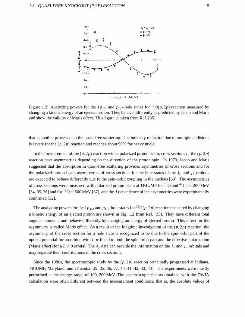
2.3.5 Trigger and data acquisition system
The data acquisition was initiated by the trigger signals from the GR and LAS scintillators. The readout
electronics and trigger systems of the focal plane scintillators for the GR andLAS are illustrated in
Fig. 2.13 and Fig. 2.14, and were placed near the focal planes of the GR and LAS, respectively. Any
output of photomultiplier tube (PMT) was first divided into two signals and onewas discriminated by
a constant fraction discriminator (CFD) and the other was sent to a FERA (Fast Encoding Readout
ADC (analog-to-digital converter);LeCroy 4300B) module. One of the CFD outputs was transmitted
to the TDC (time-to-digital converter) system that consists of TFCs (Time to FERA Converter;LeCroy
4303) and FERAs. A coincidence signal of two PMT-outputs on both sidesof the same scintillator was
generated by a Mean-Timer circuit, in which the times of two signals were averaged. Thus, the position
dependence of output timing caused by the difference of the propagation time in the long scintillator
was minimized.
The trigger system was constructed with LeCroy 2366 universal logic modules (ULM) with field
programmable gate-array (FPGA) chips. As shown in Figs. 2.13 and 2.14,the trigger system received
signals from the outputs of Mean Timers and generated the GR and LAS trigger under the condition that
signals from PS1 and PS2 coincide internally. In the LAS, PS1 or PS2 was generated when there was
at least one signal of three Mean Timer outputs corresponding to up, middle, and down scintillators.
The GR trigger gave the gate signals of ADC modules and start or stop signalsof TDC modules for

24 CHAPTER 2. EXPERIMENT
12.8mm
X1X2 Y1Y2D
GR(LAS)
Center of
Scattering Chamber
D = 542.3 mm / 551.3 mm ( E168 )GR / LAS
D = 544.1 mm / 546.0 mm ( E217 )GR / LAS
To the GR
(LAS)
Figure 2.11: Geometrical relation of anode planes of the MWPC and the center of the scattering cham-ber.
charged particle
cathode foil
cathode foil
sense wire
6.4
mm
6.4
mm 2.02mm
Figure 2.12: Structure of each wire plane of the MWPCs.
the GR focal plane detectors, while the LAS trigger was used as the ADC gatesignals and the TDC
start or stop signals for the LAS focal plane detectors. The coincidencetrigger of the GR and LAS was
also generated in the 2366 module at the GR side, where the output timing was determined by the LAS
trigger. The logic diagram for coincidence event of the GR and LAS is shown in Fig. 2.15. The (p,2p)
event was measured by GR+LAS coincidence mode, and a GR single event and a LAS single event
were also measured under the sampling condition. The main trigger output started the data acquisition
system.
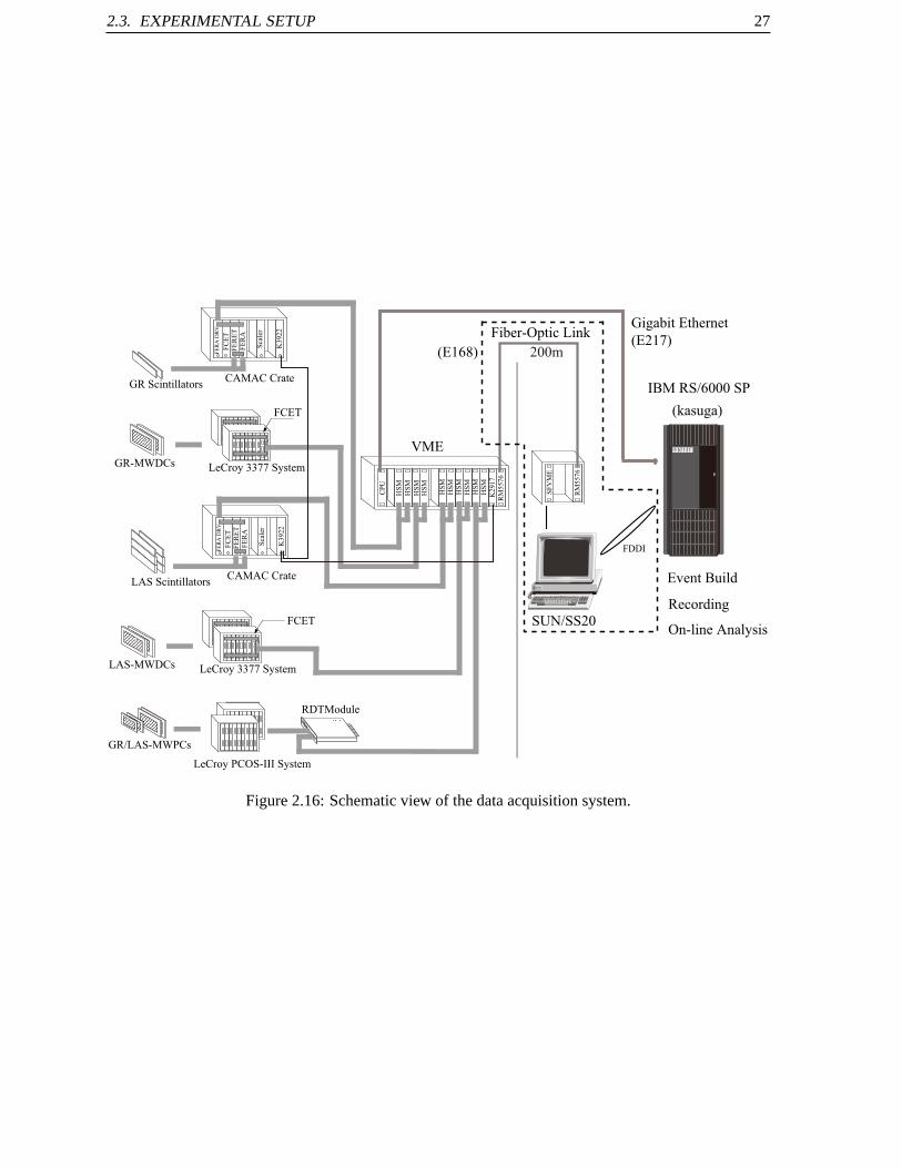
A schematic diagram of the data acquisition (DAQ) system [64, 65] is shown inFig. 2.16. The
digitized data of the TDCs and ADCs for the detectors were transferred in parallel via the ECL bus to
the high speed memory modules (HSM) in the VME crate. The flow controlling event tagger module
(FCET) [66], that was installed in each CAMAC crate for TDCs and ADCs,attaches the event header,
event number, and input register words to the data from the LeCroy FERAand FERET system for the
subsequent event reconstruction, and transfers the data via the ECL bus. Similarly, the rapid data transfer
module (RDTM) [67] manages the data from the LeCroy PCOS III system. The CAMAC actions are
2.3. EXPERIMENTAL SETUP 25
excluded in this data transfer process. In the present measurements, theDAQ system treated the data
from the GR-MWDCs, the GR-scintillators, the LAS-MWDCs, the LAS-scintillators, and the MWPCs
for GR and LAS, in parallel. Each transfer line has two HSMs, which work as a double-buffer and
reduce dead time in transferring buffered data.
The stored data in the HSMs were moved to a reflective memory module of RM5576 through the
VME bus by an MC68040 based CPU board, and the data in the RM5576 wasautomatically copied
to another RM5576 module in the counting room through the link of optical fibercables. A SUN
workstation read the data from the RM5576 in the counting room and transferred them to an IBM
RS/60000 workstation via an FDDI network. This data transfer method with reflective memory modules
and optical fiber cables was used in the beamtime of E168. In the beamtime of E217, new data transfer
method, which directly transfers the data to the workstation by a gigabit Ethernet, was installed and
used. The data was stored in the large hard disk connected to the workstation. The event reconstruction
and online data analysis were also performed on this computer.
Beam current was adjusted so that the live time of the DAQ system was kept at almost 80–90%.
PS1-L
PS1-R
Mean
Timer
CFD PS1
CFD
delay
delay
35
17PS1
PS2
Timing Chart
t (ns)
T F
C
F E
R A
F E
R A
PS2-L
PS2-R
Mean
Timer
CFD PS2
CFD delay
delay
GR trigger
Figure 2.13: Logic diagram for the GR focal plane detectors.

26 CHAPTER 2. EXPERIMENT
50
15
PS1
PS2
Timing Chart
t (ns)
PS1U-L
PS1U-R
Mean
Timer
CFD
PS1
CFD delay
delay
T F
C
F E
R A
F E
R A
delay
PS1U-L
PS1U-R
Mean
Timer
CFD
CFD
PS1D-L
PS1D-R
Mean
Timer
CFD
CFD
PS2U-L
PS2U-R
Mean
Timer
CFD
CFD delay
PS2U-L
PS2U-R
Mean
Timer
CFD
CFD
PS2D-L
PS2D-R
Mean
Timer
CFD
CFD
PS2
LAS trigger
.....
.....
Figure 2.14: Logic diagram for the LAS focal plane detectors.
1/m
1/n
GR+LAS
coincidence trigger
GR
sample trigger
LAS
sample trigger
~500
LAS
GR
Timing Chart
for GR+LAS coincidence
t (ns)LAS trigger
Sampling
Sampling
GR trigger
Figure 2.15: Logic diagram for coincidence event of the GR and LAS.
2.3. EXPERIMENTAL SETUP 27
CP
U
RM
5576
K2917
HS
M
HS
M
HS
M
HS
M
HS
M
HS
M
CP
U
HS
MH
SM
HS
M
HS
M
CP
U
Fiber-Optic Link
IBM RS/6000 SP
SUN/SS20
FDDI
Event Build
SF
VM
E
RM
5576
sun
(kasuga)
Recording
On-line Analysis
200m
GR-MWDCs
GR ScintillatorsCAMAC Crate
LeCroy 3377 System
K3922
Sca
ler
FE
RA
FE
RE
T
FC
ET
FE
RA
DR
V
GR/LAS-MWPCs
RDTModule
FCET
LeCroy PCOS-III System
LAS-MWDCs LeCroy 3377 System
FCET
LAS ScintillatorsCAMAC Crate
K3922
Sca
ler
FE
RA
FE
RE
T
FC
ET
FE
RA
DR
V
VME
Gigabit Ethernet
(E217)(E168)
Figure 2.16: Schematic view of the data acquisition system.

28 CHAPTER 2. EXPERIMENT
Chapter 3
Data Reduction
A program code ’Yosoi analyzer’ has been developed for analyzingexperimental data obtained with the
GR and/or LAS spectrometer system at RCNP. The analyzed results were stored ina HBOOK [68] file
and graphically displayed using a program PAW [69]. The data analysis was mainly carried out by using
the central computer system at RCNP, that is, IBM RS/6000SP system.
3.1 Polarization of proton beam
The beam polarization was measured by using the beam-line polarimeter 1 (BLP1) located at the first
straight beam-line section in the west experimental hall. The BLP2 was used for monitoring the transport
and polarization of the beam.
Yield (NL (NR)) in coincidence by the pair of scintillators of L(R) and L’(R’) in Fig. 2.3 for spin-up (↑)and spin-down (↓) modes are described as
N↑L = N p↑L − Na↑
L = σ0(θL)NtN↑bǫL∆ΩL(1+ Ay(θL)p↑y), (3.1a)
N↑R = N p↑R − Na↑
R = σ0(θR)NtN↑bǫR∆ΩR(1− Ay(θR)p↑y), (3.1b)
N↓L = N p↓L − Na↓
L = σ0(θL)NtN↓bǫL∆ΩL(1− Ay(θL)p↓y), (3.1c)
N↓R = N p↓R − Na↓
R = σ0(θR)NtN↓bǫR∆ΩR(1+ Ay(θR)p↓y). (3.1d)
The superscripts of↑ and↓ represent the quantities in spin-up (↑) and spin-down (↓) modes.N p and
Na are the numbers of prompt and accidental coincidence events,σ0(θ) andAeffy (θ) are unpolarized cross
section and analyzing power forp + p scattering.Nt andNb are the numbers of the target and beam
particles.py, ǫ and∆Ω are the beam-polarization in the vertical direction, the efficiency, and the solid
angle of each scintillation detector, respectively. The accidental coincidence eventNa was estimated
using the number of forward counter L(R) event coincident with the event of backward counter L’(R’)
in the next beam bunch.
The angular acceptances of the polarimeter were determined by collimating the backward protons. If
29

30 CHAPTER 3. DATA REDUCTION
there was no instrumental asymmetry, namelyǫL∆ΩL = ǫR∆ΩR = ǫ∆Ω, the beam polarization can be
expressed as follows;
p↑ =1
Ay(θ)2Q − (L + R)
L − R(3.2a)
p↓ =1
Ay(θ)
2/Q −(
L−1 + R−1)
R−1 − L−1. (3.2b)
L =N↓LN↑L
, R =N↓RN↑R
, Q =N↓bN↑b
(3.3)
The scattering angles of forward and backward protons for a 392 MeVproton beam were set atθlab =
17 and θlab = 69.7, respectively, The effective analyzing power ofAy(17) = 0.44 ± 0.01 for pp
scattering from the polyethylene target was used in Eq. (3.2) to determine thebeam polarization. This
value of Ay(17) for 392 MeV was previously calibrated in comparison with two polarization values
measured before and after the ring cyclotron for a vertically polarized proton beam. The beam polar-
ization before the acceleration by the ring cyclotron, which was measured by BLP-N between the AVF
and ring cyclotrons, was determined from the asymmetry for the12C(p, p) elastic scattering with the
analyzing power data of the12C(p, p) elastic scattering measured at RCNP [70]. The beam polarization
of 60–70% was achieved in the experiments.
3.2 Particle Identification
Combination of the time of flight (TOF) through the spectrometer and the∆E signals of the plastic
scintillators provided the particle identification at the focal plane of the spectrometers. Photons from
the scintillators were detected by PMTs attached on both the left and right sides. The photon number is
attenuated due to the absorption by the scintillator material during the transmission. The photon number
I can be described as a function of the path lengthx,
I(x) = I0 exp(
− xl
)
, (3.4)
whereI0 is the initial photon numbers andl is the attenuation length of the scintillator material. Suppose
the distances between the emitting point of the photons and the left/right PMTs arexL and xR, the
geometrical meanI of the photon numbers at both sides is
I =
√
I0 exp(
− xL
l
)
· I0 exp(
− xR
l
)
= I0 exp(
− xL + xR
2l
)
= I0 exp(
− L2l
)
. (3.5)
whereL = xL + xR is the length of the scintillator. Eq. (3.5) shows thatI is independent on a position
where a particle hits and becomes a good measure of energy deposition to thescintillator. Since the
energy loss of the charged particles in the scintillator material is described bythe well-known Bethe-
Bloch formula, theI spectra are useful for the particle identification. Figure.3.1 shows the∆E signal
from PS1 of the GR. The peaks corresponding to protons and deuterons are recognized.

3.2. PARTICLE IDENTIFICATION 31
1
10
102
103
104
105
106
0 200 400 600 800 1000 1200 1400 1600
∆E1 (ch.)
Co
un
ts
Proton
Deuteron
Figure 3.1: Energy loss spectrum from the PS1 of the GR, which is the mean of the pulse-height signalsof the left and right PMTs.
Figure 3.2 (a) shows the TDC spectrum that indicates the time difference between the mean-time
signal from PS1 of the GR and the RF signal from the AVF cyclotron. The RF signal, which was filtered
at the half rate with a rate divider module, stopped the TDC and provided a periodic spectrum. Both
of the two prominent peaks at 550 ch and 1050 ch in Fig 3.2 (a) indicate the spectra of proton trigger
events, and the difference between the two peaks in TDC channel corresponds an interval of 60-ns
period between beam bunches. The influence of the momentum acceptanceof the spectrometer in the
TDC spectrum was corrected by using the trajectory angle and the position at the focal plane, as seen
in Fig. 3.2 (b). The time difference between the mean-time signal of a scintillator and the RF signal
from the ring cyclotron reflects the time that the scattered particle takes to reach the scintillator from the
target through the spectrometer. Since the particles have different velocities that depend on their masses
under the same momentum condition, the TDC spectra of this time difference provides information on
the masses of the particles.
Protons were identified by setting gates on the TDC spectra because the∆E peak of proton has a long
tail at higher∆E region. The∆E spectra of the PS1 scintillator was also used for the particle identifi-
cation to eliminate theγ-ray contribution. These gates identifying proton are schematically displayed
in the two-dimensional scatter plot of the corrected TDC and∆E of the GR in Fig. 3.3. The proton
identification of the LAS was performed in the identical way.
In the analysis of set1a and a part of set2a in Table 2.1, however, protonevents were identified with
only the∆E spectra because of the lack of the TDC data. In the part of set2a that includes the TDC
information in the data, both of the particle identification were compared, and theyield identified with
only the∆E spectra was 0.5% smaller than that with the TDC and∆E spectra. Since the∆E spectra of
the PS1 in set1a shows a similar shape to that in set2a, the influence of the lack of the TDC data for the
particle identification in set1a is expected to be as small as that in set2s.

32 CHAPTER 3. DATA REDUCTION
11010
210
310
410
510
610
710
8
0 200 400 600 800 1000 1200 1400TDC (ch.)
Co
un
ts
(a)
11010
210
310
410
510
610
710
8
0 200 400 600 800 1000 1200 1400TDC
corr. (ch.)
Co
un
ts
(b)D
eute
ron
Pro
ton
Deu
tero
n
Pro
ton
Pro
ton
Pro
ton
Deu
tero
n
Deu
tero
n
Figure 3.2: (a):TDC spectrum that indicates the time difference between the mean-time signal from PS1of the GR and the RF signal from the AVF cyclotron. The RF signal was filtered at the half rate. (b):TDC spectrum corrected by the trajectory angle and the position at the focal plane so that the influenceof the momentum acceptance of the spectrometer on the TDC is eliminated.
3.3 Subtraction of accidental coincidences
The proton beam from the cyclotron has a time structure of approximately 60-ns period between bunches.
To estimate the yield of accidental events, coincidence between the signals ofthe GR and LAS from
adjacent beam bunches was allowed by increase in the width of the trigger signal of the GR. The yield of
the true (p,2p) events, which must originate from the same beam bunch, was estimated by subtracting
the yield of the accidental events from the yield of the coincident events in thesame beam bunch.
A TDC spectrum for the time difference between the trigger signals of the GR and LAS is shown in
Fig. 3.4. Each peak corresponds to one beam bunch. A prompt peak includes both the true and accidental
coincidence events, while the other peaks include the accidental coincidence events. Assuming the
beam has no micro-structures, that is, the same number of protons are included in all beam bunches, the
yield of only true coincidence events can be extracted by means of subtracting the events of one of the

3.4. TRACK RECONSTRUCTION OF SCATTERED PARTICLES 33
0
500
1000
1500
0 200 400 600 800 1000 1200 1400
TDCcorr.
(ch.)
∆E
1 (
ch.)
Deu
tero
n
Deu
tero
n
Pro
ton
Pro
ton
Figure 3.3: Two-dimensional scatter plot of the corrected TDC and∆E1 of the GR. The events enclosedby the solid lines are recognized as the proton events.
accidental bunch from those of the true bunch.
3.4 Track reconstruction of scattered particles
3.4.1 Multi-wire drift chambers
The trajectories of charged particles entering the focal planes of both spectrometers were determined
with the GR and LAS-MWDCs. As shown in Fig. 3.5, the positionp of an incident charged particle
at an anode plane of the MWDC is determined from the drift lengthsdi−1, di of at least more than two
wires in the same cluster. A cluster means that it has at least two adjacent hit wires. Since theX- and
γ-rays mostly hit only one wire, background events by photons can be muchexcluded. When|di| is the
minimum in a cluster with three hit wires, the positionp is simply calculated as
p = pi + lWSdi−1 + di+1
di−1 − di+1, (di−1 > 0, di+1 < 0) (3.6)

34 CHAPTER 3. DATA REDUCTION
0
1000
2000
3000
4000
x 10 2
600 800 1000 1200 1400
TDC (ch.)
Co
un
ts
Figure 3.4: TDC spectrum for the time difference between the GR and LAS trigger signals in a mea-surement of the40Ca(p,2p) reaction.
p
i-1
d i di+1
ChargedParticle
Cathod Plane
Anode Wires
Cathod Plane
Sense Wire
d
Figure 3.5: position in a plane of MWDC
wherepi is the position ofi-th wire, lWS is the sense wire spacing, and a negative value is taken fordi+1
because electrons moving to (i − 1)-th wire and (i + 1)-th wire drift in the opposite direction. In the
standard setting of both the GR and LAS-MWDCs, particles with correct trajectories usually hit more
than three sense wires. The incident angle (θ) are also roughly estimated by tanθ = (di−1−d+i + 1)/2lWS
with the angular resolution of about 2. The drift velocity is almost constant but it considerably deviates
near the sense wires due to the steep gradient of the electric field. Since theTDC value only gives the
drift time of each wire, one must convert this to the drift length. The so-called x− t calibration was made
for each wire plane using the real data taken in the present measurements.Typical drift velocity of the
uniform region is about about 48µm/ns.
The residual distribution defined as
Residual =di−1 + di+1
2− di (3.7)
was used for the estimation of the resolution, and for all planes of the GR andLAS- MWDCs, the
resolutions were less than 400µm (FWHM). The position resolutionδp depends on the incident angle

3.4. TRACK RECONSTRUCTION OF SCATTERED PARTICLES 35
X
z
z’x’
X1-plane
X2-plane
U1-plane
U2-plane
ΘVDC
y, y’
(x’,y’)
Incident particle
Figure 3.6: Coordinate systems for the ray-tracing with two MWDCs.
and is mostly better than the residual resolution because the intrinsic resolutionδdi of each wire is√
6/3
of the residual distribution, which is deduced from Eq. (3.7).
3.4.2 Trajectory of a charged particle
Two sets ofX andU positions of anode planes can completely determine the three dimensional trajectory
of the charged particle. The wire configurations of theX-planes andU-planes of the GR and LAS-
MWDCs are shown in Figs. 2.7 and 2.9.
We define two coordinate systems: the central-ray coordinate in which thez-axis is the momentum
direction of the central ray and the focal-plane coordinate in whichz′-axis is perpendicular to the anode
planes of the MWDCs, as shown in Fig. 3.6. Thez − x andz′ − x′ planes are the median plane of the
spectrometer. In both coordinate systems, the center of the X1-plane is taken as the origin.
In the focal-plane coordinate system, the horizontal and vertical positions(x′,y′) and angles (θ′x =dx′dz′ ,
θ′y =dy′
dz′ ) of an incident particle are calculated frompx1, pu1, px2, and pu2, that are obtained using

36 CHAPTER 3. DATA REDUCTION
Eq. (3.6).
tanθ′x =px2 − px1
LDC, (3.8)
tanθ′u =pu2 − pu1
LDC, (3.9)
tanθ′y =tanθ′xtanψ
− tanθ′utanψ
(3.10)
x′0 = px1 (3.11)
u0 = pu1 − z′u1 · tanθ′u (3.12)
y′0 =x′0
tanψ−
u′0tanψ
(3.13)
whereLDC = z′x2− z′x1 = z′u2− z′u1 is the distance of two MWDCs,ψ is the tilting angle of U-planes, and
x′0, y′0 are the horizontal and vertical positions at thez′0 plane.LDC was 250 mm for the GR and 164 mm
for the LAS. When the position resolutionδp is 300µm and the multiple scattering effect is neglected,
the horizontal angular resolution is given as (0.3√
2/250)·cos2 θGR ∼ 0.85 mrad for the GR (θGR ∼ 45)
and (0.3√
2/164)·cos2 θLAS ∼ 0.89 mrad for the LAS (θLAS ∼ 54) at FWHM, respectively. The vertical
position and angular resolutions are about two times worse than those in the horizontal direction. The
position resolution of 300µm corresponds to about 10 keV for the GR and 10–20 keV for the LAS
depending on the magnetic field, and they are smaller than the energy spreadof the beam (∼ 200 keV)
in the present experiments.
In the central-ray coordinate, the horizontal and vertical angles are converted as
θx = θ′x − ΘVDC (3.14)
tanθy = tanθ′x cosΘVDC (3.15)
whereΘVDC is the tilting angle of the MWDC for the GR (45) or LAS (54). Using the ion-optical
matrix, one can trace these angles back to the scattering angles on the target.The focal plane of the
GR almost agreed with the X-plane of MWDC1, and small aberrations were empirically corrected by
looking at some two dimensional plots like anx − θ correlation spectrum. In the case of the LAS, the
momentum deviation and scattering angle relative to the central ray was obtained from the trajectory at
the focal plane by calculating the 4th-order matrix.
3.4.3 Efficiency of the MWDC
Efficiency of the MWDC was estimated by using (p,2p) events that a proton is detected with both of the
GR and LAS. Estimation of efficiency of the MWDC needs events that a proton surely goes through the
MWDC. (p,2p) events were identified by the following condition in case of the estimation of tracking
efficiency of the GR-MWDCs,
I True coincidence between the GR and LAS ( TDC between the GR and LAS )

3.5. MULTI-WIRE PROPORTIONAL CHAMBERS 37
II Identification of a proton for the LAS (∆E and TOF )
III Success in a track reconstruction with the LAS-MWDCs
IV Identification of a proton for the GR (∆E and TOF)
TOF is raw TDC data which is not corrected by information from the GR-MWDCs.
V Central region of the GR-MWDC
Position information obtained by a trigger scintillation counter was used.
We used the events that satisfy all the conditions I–V as a sample. For this sample, the number of the
events that a track reconstruction was succeeded with the GR-MWDCs wascounted; the efficiency was
evaluated as the ratio of this number to the number of the sample. The efficiency of the GR-MWDCs
was about 95%. The efficiency of the LAS-MWDC was estimated in the same way by replacing a role
of the GR and LAS, and was 80–85%.
3.5 Multi-wire proportional chambers
Each MWPC at the entrance of the spectrometer was used to determine the scattering angle of the
charged particle that comes to the focal plane. The LeCroy PCOS III system provides hit-wire informa-
tion by the address of the cluster centroid and the width of the cluster. The cluster centroid with the odd
hit wires is given as the wire position at the center of the hit wires, and that with the even hit wires is
given as the position between two wires with a half bit address. The address of the cluster centroid is
obtained in the accuracy of half pitch of the sense wire, that is, it is determined in the width of 1.01 mm
∼ ±0.505 mm. The scattering angle of the particle was determined from the horizontaland vertical
positions at the MWPC, assuming that the particle comes from the center of the target. In the present
analysis, each anode plane was required to have only one cluster to determine the position of charged
particle in the anode plane. If the angular resolution is estimated with the wire spacing of 2.02 mm since
the events with only one hit wire in a cluster is predominant, it is approximately
√
(
2.02550
)2
+
(
1550
)2
∼ 0.22 ∼ ±0.11, (3.16)
where the source width is assumed to be 1 mm in diameter and 550 mm is a approximatedistance from
the center of the scattering chamber to an anode plane.
For an estimation of the efficiency of the MWPC, we used the events that a track reconstruction with
the MWDC succeeds for a proton at the focal plane. For this sample, the number of the events that a
scattering angle was obtained was counted; the efficiency was evaluated as the ratio of this number to
the number of the sample. The efficiency of the GR-MWPC was about 90% and that of the LAS-MWPC
38 CHAPTER 3. DATA REDUCTION
was about 40–60%. The multi-cluster events decreased the efficiency of the LAS-MWPC because the
LAS-MWPC has a large active area.
3.6 Solid angles
The horizontal scattering angle obtained with the MWDCs at the focal plane was used for particles
comig to the GR, whereas, the horizontal scattering angle obtained with the MWPC at the entrance of
the LAS was used for particles comig to the LAS because the resolution of the horizontal stattering
angle obtained with the MWDCs at the LAS was worse than that with the MWPC dueto the multiple
scattering. The vertical scattering angles obtained with the MWPCs were used for particles coming to
the GR and LAS.
Figure 3.7 shows the two dimensional scatter plots of the horizontal (dx/dz) and vertical (dy/dz)
scattering angles for protons analyzed with the GR and LAS.
The solid angle for the GR was determined by the lead collimator as 2.4 msr. Although the lead
collimator was installed at the entrance of the LAS to determine the solid angle in a rectangle shape, the
scattering angle for the LAS shown in Fig. 3.7 (b) doesn’t show a rectangle but a hexagonal shape. The
chipped corners in Fig. 3.7 (b) indicates that a part of protons which pass through the collimator stopped
in the LAS. The solid angle for the LAS eliminated the chipped corners was estimated as 19.1 msr,
which is a little smaller than 20.0 msr determined by the lead collimator.
When the LAS was set at 56.41, pp scattering event also measured at large scattering angle part in
the solid angle for the LAS. As cross section forpp scattering is much larger than (p,2p) reaction, just
a tiny part of the protons frompp scattering that lost its energy in the spectrometer possibly interfere
with the spectrum of (p,2p) reaction. Therefore, only at this LAS angle setting (set1a–c), the partof
the solid angle that is larger than 58.41 for the horizontal scattering angle was eliminated, and its solid
angle 16.4 msr was used.
3.7 Normalization due to the trigger efficiency of the scintillation detec-tors
For a charged particle, a passage through the two plastic scintillation counters and an aluminum plate,
which is placed between the scintillators, provides a trigger signal at each focal plane. The detection
efficiency of the scintillation counter system for the GR was previously measuredwith a proton beam
at 300 MeV changing the thickness of the aluminum plate, and the measured results show that the
efficiency decreases as the thickness of the aluminum plate increases [71]. The inefficiency must be pro-
portional to the total reaction cross section between proton and materials. The proton-27Al total reaction
cross section is almost constant within a 10% fluctuation for the proton energy of below 400 MeV [72].
Therefore, the proton-energy dependence of the inefficiency was considered to be constant in the energy

3.7. NORMALIZATION DUE TO THE TRIGGER EFFICIENCY OF THE SCINTILLATIONDETECTORS 39
-4
-2
0
2
4
-2 0 2
dx/dz (deg)
dy/d
z (d
eg)
(a)
-10
-5
0
5
10
-5 -2.5 0 2.5 5
dx/dz (deg)
dy/d
z (d
eg)
(b)
Figure 3.7: Two dimensional scatter plot of the horizontal and vertical scattering angles of protonsanalyzed with the GR (a) and LAS (b).
region of the present (p,2p) measurement. The inefficiency of the detection for the GR system, which
used the aluminum plates with a thickness of 10 mm, was estimated as ¯ǫGR = 2.2 ± 0.2% including
the uncertainty of 10% from the energy dependence of the total reaction cross section. The inefficiency
of the scintillator-detection system for the LAS, which used the aluminum plates with a thickness of
3 mm, was estimated as ¯ǫLAS = 1.4± 0.1% by interpolation from the measurement results for the GR.
Combined both the inefficiencies, the detection efficiency by the scintillation detectors for the (p,2p)
measurement was estimated by
ǫGR×LAS = (1− ǫGR) × (1− ǫLAS ) = 96.4± 0.3 %. (3.17)
This efficiency is due to only the scintillation detectors, which provide a trigger for DAQsystem, but
it doesn’t include the wire-counter efficiencies. The correction using this efficiency was applied on the
yield for the (p,2p) measurement.

40 CHAPTER 3. DATA REDUCTION
3.8 Separation energy of40Ca(p, 2p)39K reaction
In each of the spectrometers, the horizontal position at the focal plane corresponds to the momentum
deviation from the central momentum in the spectrometer owing to the ion-optics property. The mo-
mentum of the particle at the focal plane was obtained from the horizontal position and Bρ value for the
central ray of the spectrometer. The energy loss for protons in the air between the scattering chamber
and the spectrometer and in the MWPC was corrected using Bethe-Bloch formula. The momentum
of the residual nucleus was calculated using the momentum conservation law.The separation energy
was obtained via Eq. (2.1). The two dimensional scatter plot of the energiesof coincidence two pro-
tons measured with the GR and LAS and the separation-energy spectrum in the 40Ca(p,2p) reaction at
T0 = 392 MeV are shown in Fig. 3.8(a) and (b) The thick locus lines that correspond to the transitions
to the ground and lower excited states in39K can be seen in Fig. 3.8(a). Several discrete states, such as
the ground state (3/2+) and the first excited state (2.52 MeV 1/2+), are observed in Fig. 3.8(b).
3.9 Cross sections and analyzing powers
The differential cross section of the (p,2p) reaction in the laboratory system is written as
d4σ
dΩ1dΩ2dT1dT2=
YQAǫη∆Ω1∆Ω2∆T1∆T2
, (3.18)
whereY is the (p,2p) coincidence yield,Q is the total number of protons in the incident beam,A is
the number of target particles per unit area,ǫ is the detection efficiency, andη is the live time ratio of
the data acquisition system.∆Ω1,2 are the solid angles of the spectrometers of the GR (1) and LAS (2),
and∆T1 and∆T2 are the energy range of the proton detected with the GR and LAS.∆T1 = 8 MeV and
∆T2 = 0.1 MeV were used for the separation-energy spectra in Chapter 5.
For a certain separation energyEsepof the (p,2p) reaction, the differential cross section of
d3σ
dΩ1dΩ2dT1=
YQAǫη∆Ω1∆Ω2∆T1
, (3.19)
is used to show its recoil momentum distribution.∆T1 = 4 MeV was used for the recoil momentum
distributions.
For pllarized proton beam, the yields for spin-up (↑) and spin-down (↓) modes are described as
Y↑ =d3σ
dΩ1dΩ2dT1(1+ p↑)Q↑Aǫ↑η↑∆Ω1∆Ω2∆T1, (3.20)
Y↓ =d3σ
dΩ1dΩ2dT1(1− p↓)Q↓Aǫ↓η↓∆Ω1∆Ω2∆T1. (3.21)

3.9. CROSS SECTIONS AND ANALYZING POWERS 41
80
100
120
140
160
240 250 260
T1 (MeV)
T2 (
MeV
)39K (g.s.) 3/2 +
(a)
0
1000
2000
3000
4000
0 20 40
Esep
(MeV)
Counts
39K (g.s.)
3/2+
(b)
1/2+
2.52
Figure 3.8: (a): Two dimensional scatter plot of the energies of coincidence two protons measured withthe GR and LAS in the40Ca(p,2p) reaction atT0 = 392 MeV. (b): Separation-energy spectrum for the40Ca(p,2p) reaction. Separation energy spectrum
The superscripts of↑ and↓ represent the quantities in spin-up (↑) and spin-down (↓) modes. The
differential cross section and analyzing power are written as
dσdΩ1dΩ2dT1
=p↓N↑ + p↑N↓
p↑ + p↓1
A∆Ω1∆Ω2∆T1, (3.22)
Ay =N↑ − N↓
p↓N↑ + p↑N↓, (3.23)
where
N↑ =Y↑
Q↑ǫ↑η↑, N↓ =
Y↓
Q↓ǫ↓η↓. (3.24)
42 CHAPTER 3. DATA REDUCTION
3.10 pp-scattering
To examine the absolute value of cross sections measured with the system thatconsists of the WS
beamline, the GR and LAS spectrometers, and the focal plane detectors,pp scattering was measured at
25.5 for the GR and at 60.0 for the LAS with 9.2 mg/cm2 polyethylene targets. The uncertainties of the
angle settings for the GR and LAS are quite smaller than 0.1. Since the solid angle and the momentum
acceptance of the LAS are larger than those of the GR, the acceptance ofpp scattering measurement
was determined by the GR.
The separation energy defined with only the energies of two scattered protons in the final state as
E′sep= T0 − T1 − T2 was used to identifypp scattering event.E′sep must be 0 in case ofpp scattering.
The analyzing power was obtained in the same way as that for the (p,2p) reaction.
The measured cross section ofpp scattering was 15.52± 0.28 mb/sr, which differs by 2.3% from
theSAID [73, 74] calculation value of 15.89 mb/sr. The value of 15.89 mb/sr was evaluated by folding
over the solid-angle acceptance, as was same as the following calculation value of Ay. The difference of
2.3% between the measured cross section and theSAID calculation value is as small as the uncertainty
of the thickness of polyethylene target (2%). The measured analyzing power Ay was 0.336±0.005. The
difference between the measured value and theSAID calculation value ofAy = 0.365 is 0.029 and it is
small enough for the following discussion.

Chapter 4
Analysis
We utilized the spectrum at the set1 for the analysis of the discrete peaks, and those at set2–5 for the
analysis of the broad spectrum region. To deduce spectroscopic factors and to compare the recoil-
momentum distribution of the cross section and analyzing power with theoreticalcalculation, DWIA
calculation was carried out.
4.1 Distorted wave impulse approximation calculation
The cross sections and analyzing powers were calculated for the40Ca(p,2p)39K reaction using a DWIA
codeTHREEDEE[75].
The cross section for the quasi-elastic scattering is calculated assuming thatthe quasi-elastic scatter-
ing is aN–N scattering process in a target nucleus. The program codeTHREEDEEincludes spin-orbit
effects in distorting potentials and makes the factorization approximation in separating the matrix el-
ements of the two-body transition operator outside the distorted wave integral.When we consider a
quasi-free reactionA(a, cd)B, whereA = B + b, the cross section can be written as [75]
d3σ
dΩcΩddEc
=2π~vωBC2S
∑
ρaρ′cρ′′d
JM
1(2J + 1) (2S a + 1)
∣
∣
∣
∣
∣
∣
∑
σaσ′cσ′′d
Λσb
(2L + 1)1/2 (LΛS bσb|JM) T LΛσaσ
′cσ′′d
ρaρ′cρ′′d
〈σ′cσ′′d |t|σaσb〉∣
∣
∣
∣
∣
∣
2
,
(4.1)
whereS a = S b =12 are the spins of the particlesa andb, v is the incident velocity,ωB is the phase space
factor, andC2S is the spectroscopic factor.J, M are the total angular momentum quantum numbers of
particleb. The quantitiesL andΛ are the orbital angular momentum carried byb and its projection.
The two-body transition operatort is separated outside the distorted wave integral by the factorization
approximation. The spin matrices are given in the different coordinates where the directions of propa-
gation of particlesa, c, andd are z, z′, andz′′ axes. Spin projections are denoted asρi. The quantity
43
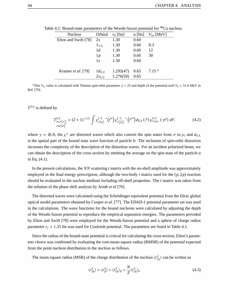
44 CHAPTER 4. ANALYSIS
Table 4.1: Bound-state parameters of the Woods-Saxon potential for40Ca nucleus.
Nucleus Orbital r0 [fm] a [fm] Vso [MeV]Elton and Swift [78] 2s 1.30 0.60
17/2 1.30 0.60 8.31d 1.30 0.60 121p 1.30 0.60 301s 1.30 0.60
Krameret al. [79] 1d3/2 1.295(47) 0.65 7.15a
2s1/2 1.276(59) 0.65
aThis Vso value is calculated with Thomas spin-orbit parameterλ = 25 and depth of the potential-wellV0 = 51.6 MeV inRef. [79].
T LΛ is defined by
T LΛσaσ
′cσ′′d
ρaρ′cρ′′d
= (2+ 1)−1/2∫
χ(−)σ′cρ
′c
∗ (~r ′)
χ(−)σ′′d ρ
′′d
∗ (~r ′′)
φLΛ(
~r)
χ(+)σaρa
(
γ~r)
d~r, (4.2)
whereγ = B/A, theχ± are distorted waves which also convert the spin states fromσ to ρ, andφLΛ
is the spatial part of the bound state wave function of particleb. The inclusion of spin-orbit distortion
increases the complexity of the description of the distortion waves. For an incident polarized beam, we
can obtain the description of the cross section by omitting the average on the spin state of the particlea
in Eq. (4.1).
In the present calculations, theNN scatteringt matrix with the on-shell amplitude was approximately
employed in the final energy prescription, although the two-bodyt matrix used for the (p,2p) reaction
should be evaluated in the nuclear medium including off-shell properties. Thet matrix was taken from
the solution of the phase shift analysis by Arndtet al [76].
The distorted waves were calculated using the Schrodinger equivalent potential from the Dirac global
optical model parameters obtained by Cooperet al. [77]. The EDAD-1 potential parameter set was used
in the calculations. The wave functions for the bound nucleons were calculated by adjusting the depth
of the Woods-Saxon potential to reproduce the empirical separation energies. The parameters provided
by Elton and Swift [78] were employed for the Woods-Saxon potential anda sphere of charge radius
parameterrc = 1.25 fm was used for Coulomb potential. The parameters are listed in Table 4.1.
Since the radius of the bound-state potential is critical for calculating the cross section, Elton’s param-
eter choice was confirmed by evaluating the root-mean-square radius (RMSR) of the potential expected
from the point nucleon distribution in the nucleus as follows.
The mean-square radius (MSR) of the charge distribution of the nucleus〈r2ch〉 can be written as
〈r2ch〉 = 〈r
2p〉 + 〈r2
ch〉p +NZ〈r2
ch〉n (4.3)
4.1. DISTORTED WAVE IMPULSE APPROXIMATION CALCULATION 45
where〈r2p〉, 〈r2
ch〉p, and〈r2ch〉n denote the MSRs of the point proton distribution in the nucleus, the charge
distribution of the proton, and the charge distribution of the neutron, respectively. Z andN indicate the
number of protons and neutrons in the nucleus. The RMSRs of the chargedistribution of the proton
and of the40Ca nucleus are〈r2ch〉
1/2p = 0.8791 fm [80] and〈r2
ch〉1/2Ca = 3.4764 fm [80], respectively. The
MSR of the neutron charge distribution〈r2ch〉n is−0.1149 fm2 [80]. Note that the negative value of〈r2
ch〉ncomes from the negative charge distribution in the larger-radius region ofthe neutron. From Eq. (4.3),
the RMSR of the proton distribution in the40Ca nucleus is estimated as
〈r2p〉1/2 =
(
〈r2ch〉Ca− 〈r2
ch〉p −NZ〈r2
ch〉n)1/2
= 3.38 fm. (4.4)
The MSR of the potential in the nucleus can be considered as the sum of the MSR of the nucleon
distribution in the nucleus and that ofNN interaction range. Assuming the effective interaction range
of 〈r2int〉 = 5.78 fm2 calculated from the mass-number-dependent formula〈r2
int〉 = (0.132± 0.013)A2/3 +
(4.24± 0.24) fm2 [81], we evaluated the RMSR of the40Ca potential as
〈r2pot〉1/2Ca =
(
〈r2p〉 + 〈r2
int〉)1/2= 4.15 fm. (4.5)
The MSR of the proton distribution is used instead of the MSR of the nucleon distribution because40Ca has the same number of protons and neutrons. It was confirmed that theRMSR of 4.14 fm for
the Woods-Saxon potential with the Elton parameter is in good agreement with theestimated RMSR of
4.15 fm for the40Ca potential expected from the point nucleon distribution.
To compare the measured and calculated cross sections, the cross sections calculated with the DWIA
code were averaged over the angular and momentum acceptances of the spectrometers.
Since the deep-hole states induced by nucleon knockout reactions fromdeeply bound orbitals stay far
above the particle-decay threshold and have short lifetimes, these states have large widths and overlap
each other. If we assume that the cross sections for different hole states do not interfere coherently with
each other, the total cross section can be described by the superpositionof cross sections for different
hole states by the (p,2p) reaction. Since the recoil-momentum distribution of the (p,2p) reaction cross
section predominantly depends onL, a superposition of the cross sections for the (p,2p) reaction from
differentL orbitals was used for a fitting to the experimental recoil-momentum distribution data.The
single-particle-hole strength for each orbital was obtained by the fitting. This technique is known as
l-decomposition [82] or multipole decomposition analysis (MDA).
Figure4.1 shows recoil momentum distributions of cross sections for some single hole states calcu-
lated by the DWIA code. The cross section shows characteristic recoil-momentum distribution depend-
ing on the angular momentum (L) of the hole state. When the angular momentumL increases, the
maximum position of the cross section moves to larger recoil-momentum region. The MDA utilizes this
L-dependence of cross sections.
The momentum distribution of the cross section at a separation energyEsep is written in terms of the
(p,2p) cross sectionσDWIAα (Esep,T1) for the single-particle-hole state obtained from a DWIA calcula-

46 CHAPTER 4. ANALYSIS
0
0.02
0.04
0.06
0.08
-300 -200 -100 0 100 200 300
P3 [ MeV/c ]
d3 σ
/dΩ
1dΩ
2dE
1 [ µ
b/S
r2M
eV ]
1s1/2
(×0.5)
1p3/2
1p1/2
1d5/2
Figure 4.1: Recoil-momentum distributions of the cross sections for the 1s1/2-, 1p3/2-, 1p1/2-,and 1d5/2-hole states by DWIA calculations. They were calculated with spectroscopicfactorsof 1 at a separation energy 15 MeV in a certain kinematical condition.
tion as follows:
σcalc(Esep,T1) =∑
α
S α(Esep)σDWIAα (Esep,T1), (4.6)
whereα indicates an occupied single-particle orbital in the nucleus, for exampleα=2s1/2, 1d5/2, etc.
S α(Esep) is the hole-state strength for the orbitalα. The quantityσ(Esep,T1) denotes the triple-differential
cross section,
σ(Esep,T1) =d3σ
dΩ1dΩ2dT1, (4.7)
whereΩ1, Ω2, andT1 represent the solid angles of the two spectrometers and the kinetic energy of one
of the scattered protons, respectively.
Theχ2 for fitting to the cross-section data is defined by:
χ2 =∑
i
σexp(Esep,T1i) − σcalc(Esep,T1i)
∆σ(Esep,T1i)
2
, (4.8)
whereσexp(Esep,T1) and∆σ(Esep,Ti) are the measured cross section and its uncertainty including the
statistical and the systematic uncertainties. From the analysis ofpp scattering in Sec. 3.10, the sys-
tematic uncertainty of 2–3% was needed, and the 5–6% uncertainty arose from the thicknesses of the
calcium targets. Therefore, we added these two kinds of uncertainties in quadrature and included the

4.2. MULTIPOLE DECOMPOSITION ANALYSIS WITHAY DATA 47
systematic uncertainty of 7% in the uncertainties for the fittings. The summation index i runs to the
number of the data and theS αs were searched to minimize theχ2 at each separation energy. The uncer-
tainties in theS αs correspond to a change of 1 inχ2 from the minimum value. The spectroscopic factor
for the orbitalα was given by summing the strengths as
S α =∑
Esep
S α(Esep). (4.9)
4.2 Multipole decomposition analysis withAy data
The cross sections of each single-particle state for spin-up and spin-down states of proton beam with po-
larizationp are written by using the cross sectionσDWIAα (Esep,T1) and the analyzing powerADWIA
y (Esep,T1)
as
σcalc↑ (Esep,T1) =
∑
α
S ασDWIAα (Esep,T1)
1+ pADWIAy α (Esep,T1)
, (4.10)
σcalc↓ (Esep,T1) =
∑
α
S ασDWIAα (Esep,T1)
1− pADWIAy α (Esep,T1)
, (4.11)
where the↑ and↓ show spin states of the proton beam.
The analyzing power at a definiteEsep is written as
Acalcy (Esep,T1)
=1p
σcalc↑ (Esep,T1) − σcalc
↓ (Esep,T1)
σcalc↑ (Esep,T1) + σcalc
↓ (Esep,T1)
=
∑
α S α(Esep)σDWIAα (Esep,T1) ADWIA
y α (Esep,T1)∑
α S α(Esep)σDWIAα (Esep,T1)
. (4.12)
In the MDA with theAy data, theχ2 for theAy data is defined as
χ2Ay=
∑
i
Aexpy (Esep,Ti) − Acalc
y (Esep,Ti)
∆Ay(Esep,Ti)
2
(4.13)
whereAexpy (Esep,T1) and∆Ay(Esep,Ti) are a measured analyzing power and the uncertainty. In the case
of MDA including the cross section and analyzing power,χ2Ay
is also included and the totalχ2 is defined
asχ2 = χ2cs+χ
2Ay
.

48 CHAPTER 4. ANALYSIS
Chapter 5
Result
5.1 Separation-energy spectra
Separation-energy spectra at the measured kinematical set1–5 are displayed in Fig. 5.1–5.5. Yields of
some part of the spectra are small due to the limits of the momentum acceptance of the spectrometers.
Vertical dotted lines in Fig. 5.3–5.5 show boundaries where the momentum acceptance is guaranteed.
Part of yields at the outside of the dotted lines are lost due to the momentum acceptance. The typical
separation-energy resolution is 750 keV at full width at half maximum (FWHM).
The spectra display the cross section as a function of the separation energy and show the distribution
of hole states. The transitions to the ground and lower excited states in39K are seen as the discrete
peaks in Fig. 5.1 and 5.2. In Figure 5.2 and 5.3, a hump is seen around 30 MeV, where the hole state of
the 1p orbital is expected from previous experiments. Over 40 MeV, the cross section decreases as the
separation energy increases, and no peak or hump cannot be seen.
Two prominent discrete peaks at 8.3 and 10.9 MeV in the separation energywere analyzed at the set1
independently because they are well isolated, and the data of the broad spectrum region at separation
energies above 12 MeV was analyzed by a multipole decomposition analysis atthe set2–5 to separate
the contribution from some hole states.
49

50 CHAPTER 5. RESULT
Figure 5.1: Separation-energy spectra at the measured kinematical set1 inTable 2.1.

5.1. SEPARATION-ENERGY SPECTRA 51
Figure 5.2: Separation-energy spectra at the measured kinematical set2 inTable 2.1.

52 CHAPTER 5. RESULT
Figure 5.3: Separation-energy spectra at the measured kinematical set3 inTable 2.1. Vertical dottedlines show boundaries where the momentum acceptance is guaranteed. Yields at the outside of thevertical dotted lines decrease due to the finite momentum acceptance of the spectrometers.

5.1. SEPARATION-ENERGY SPECTRA 53
Figure 5.4: Separation-energy spectra at the measured kinematical set4 inTable 2.1. Vertical dottedlines show boundaries where the momentum acceptance is guaranteed. Yields at the outside of thevertical dotted lines decrease due to the finite momentum acceptance of the spectrometers.

54 CHAPTER 5. RESULT
Figure 5.5: Separation-energy spectra at the measured kinematical set5 inTable 2.1. Vertical dottedlines show boundaries where the momentum acceptance is guaranteed. Yields at the outside of thevertical dotted lines decrease due to the finite momentum acceptance of the spectrometers.

5.2. RESULTS FOR DISCRETE STATES 55
5.2 Results for discrete states
The separation-energy spectrum up to 20 MeV at the set1 is shown in Fig. 5.6. Two prominent peaks are
observed at 8.3 and 10.9 MeV. The recoil-momentum distributions of the cross section and analyzing
power for these peaks are displayed in Figs. 5.7 and 5.8, respectively.The error bars that represent the
statistical uncertainties are in the symbols.
0
2000
4000
6000
0 5 10 15 20
Separation Energy [MeV]
Counts
1d3/2
2s1/2
and
1f7/2
12.0
8.3
10.9
Figure 5.6: Separation-energy spectrum of the40Ca(p,2p) reaction up toEsep =
20 MeV for the kinematical set1 (Table 2.1). Two prominent peaks are observedat 8.3 MeV and 10.9 MeV. The MDA was performed at separation energiesabove12 MeV.
In Fig. 5.7, the cross section of the first hole state has a minimum nearp3 = 0 MeV/c in the recoil-
momentum distribution. This suggests that the peak consists of a hole state of a single-particle orbital
with L , 0, as mentioned in Sec. 2.2.
In 40Ca, the orbital withL , 0 near the Fermi surface is 1d orbital. The 1d orbital is split into
the j< and j> orbitals by the spin-orbit interaction and thej> orbital is bound more deeply thanj<orbital. The j< orbital, that is, the 1d3/2 orbital ought to contribute a hole state of the first peak. The
solid curves in Fig. 5.7 show the recoil-momentum distributions for the hole state of the 1d3/2 orbital
obtained from the DWIA calculation, which are normalized to the measured cross section. The DWIA
calculation reproduces the measured cross section reasonably well. Thecalculation roughly reproduces
the dependence of the recoil momentum on the analyzing power, but the value of the analyzing power
is systematically overestimated in the entire recoil-momentum range. The spectroscopic factor deduced
as the normalization factor is listed in Table 5.1 and is over the 2J + 1 value of 4.
In Fig. 5.8, the recoil-momentum distribution of the cross section for the peak at 10.9 MeV exhibits
a maximum around 0 MeV/c, which is characteristic for a hole state of a single-particle orbital with
L = 0. Therefore, the hole state of the 2s1/2 orbital is expected to be dominant in the peak at 10.9 MeV.
Comparing with the level structure of39K [83], we see that the hole states of the 1f7/2 and 2p3/2 orbitals

56 CHAPTER 5. RESULT
Figure 5.7: Cross section (a) and analyzing power (b) of the40Ca(p,2p) reaction for the peak at 8.3 MeVas functions of the recoil momentump3. The solid line represents the DWIA calculations fitted by thespectroscopic factor for the 1d3/2 orbital. The discrepancy inAy (b) between the data and the DWIAcalculation is discussed in the text (Sec.5.2A.).
will be included in the peak as well. Since the contribution of the 2p3/2-hole state is negligible compared
with those of the 2s1/2- and 1f7/2-hole states [10], the peak at 10.9 MeV was analyzed as the sum of
the 2s1/2- and 1f7/2-hole states. We searched the best set of normalization factors for the calculated
cross sections for the 2s1/2- and 1f7/2-hole states to reproduce the measured cross sections. The result
is shown in Fig. 5.8 and the obtained spectroscopic factors are listed in Table5.1. The fitted thick solid
line for the cross section agrees well with the experimental data, but the calculated analyzing power is
larger than the measurement, which is similar to the results for the 1d3/2-hole state.
The spectroscopic factors for the valence orbitals were reported fromthe previous (p,2p) [40, 84, 85]
(e, e′p) [52] and (d,3He) [10, 52, 86] reactions as listed in Table 5.1. The values from (p,2p) reaction
have differences by its measurement angles and used distortion potentials. This implys there is uncer-
tainties in spectroscopic factors for (p,2p) reaction due to the distortion potential and the kinematical
condition. The spectroscopic factors reported by Dollet al. from the (d,3He) reaction are systematically
larger than those from the (e, e′p) reaction. However, Krameret al. reanalyzed the same (d,3He) data
in Ref. [10] and showed that the spectroscopic factors for the 1d3/2 and 2s1/2 orbitals obtained from the
(e, e′p) and (d,3He) reactions are consistent [52]. As the obtained spectroscopic factors in the present
work are larger than those consistent values from (e, e′p) and (d,3He) reaction and that for the 1d3/2-hole
state is over the 2J + 1, the obtained spectroscopic factors are probably overestimated. This leads that
the DWIA calculation underestimated the absolute cross sections.
The DWIA calculation systematically overestimates the analyzing powers as seen in Figs. 5.7 (b)
and 5.8 (b). The reduction of the analyzing power in exclusive measurements was previously observed
and discussed by Noroet al. [48], Miller et al. [45], and Hatanakaet al. [46]. Furthermore, a similar
reduction in the polarizationP was observed by Miklukhoet al. [87] and Andreevet al. [49]. These

5.3. RESULTS OF THE DEEPLY BOUND STATES 57
Figure 5.8: Results of the MDA for the peak at 10.9 MeV. The cross section(a) and the analyzing power(b) are shown as functions of the recoil momentump3. The thick solid line shows the fitted results. Thethin solid line and the dotted line show the contributions of the 2s1/2 and 1f7/2 states, respectively. Thediscrepancy inAy (b) between the data and the DWIA calculation is discussed in the text (Sec.5.2A.).
authors considered that the reduction might be caused by the influence ofthe effective mean density
on theNN interaction. The systematic discrepancies between the experimental data andthe DWIA
calculation in Figs. 5.7 (b) and 5.8 (b) possibly imply the modification of theNN interaction in the
nucleus. Although various extensive theoretical studies have been performed, no theoretical model has
succeeded in reproducing the experimental analyzing power quantitatively.
The separation of the hole states of thej> and j< orbitals by using the analyzing power data requires
the DWIA calculation reproducing the data not only qualitatively but also quantitatively. The result of
the valence orbitals are discouraging to do it.
5.3 Results of the deeply bound states
The MDA was performed for each 2-MeV bin in the separation energy region of 12–84 MeV with only
the cross section data. The hole states of the 1s1/2, 2s1/2, 1p and 1d orbitals were taken into account in
the MDA since from the naive shell-model picture they are expected to dominate in the broad spectrum
region. As hole states ofj> and j< orbitals with the sameL cannot be distinguished in the present MDA,
the single-particle-hole states were treated under the following assumptions.
Since the 1d orbital is split into the 1d3/2 and 1d5/2 orbitals and the 1d5/2 orbital is bound more
deeply than 1d3/2 orbital, the hole state of the 1d5/2 orbital is expected to dominate thed-state strength
at separation energies above 12 MeV. The relative strengths for the 1p1/2- and 1p3/2-hole states were
fixed in the ratio of 2:4 as suggested by the naive shell-model picture. Sincethe recoil-momentum
distributions of the cross sections for the 1s1/2- and 2s1/2-hole states are quite similar, the strengths

58 CHAPTER 5. RESULT
Table 5.1: Spectroscopic factors for the discrete peaks in the40Ca measurement. Krameretal. reanalyzed the previous (d,3He) data of Dollet al. in Ref. [10] in their study [52]. Thepresent result is shown with the uncertainty obtained in the fitting or MDA.
Esep[MeV] Orbital Spectroscopic factor(p,2p)
Ep = 392 MeV, RCNP, OsakaPresent work 8.3 1d3/2 4.87± 0.09
10.9 2s1/2 1.61± 0.0410.9 1f7/2 1.12± 0.06
Ep = 45.0–148.2 MeV, MarylandSamantaet al. [40] 8.33 1d3/2 3.9–6.0
10.85 2s1/2 1.0–1.6
Ep = 200 MeV, TRIUMF, Antonuket al. [36]Kudo and Miyazaki [84] 8.33 1d3/2 1.46–3.37
Mano and Kudo [85] 8.33 1d3/2 2.44–2.80(e, e′p)
NIKHEFKrameret al. [52] 8.328 1d3/2 2.58± 0.19
10.850 2s1/2 1.03± 0.07(d,3He)
Ed = 52 MeV, KarlsruheDoll et al. [10] 8.33 1d3/2 3.70
10.85 2s1/2 1.6511.15 1f7/2 0.58
Krameret al. [52] (reanalysis) 8.328 1d3/2 2.3010.850 2s1/2 1.03
Ed = 34.4 MeV,Oak RidgeHiebertet al. [86] 8.33 1d3/2 4.23
10.86 2s1/2 1.6211.15 1f7/2 0.46
for the 1s1/2- and 2s1/2-hole states cannot be distinguished by the MDA. Therefore, thes-hole state
strengths in the lower and higher separation-energy regions were assumed to be the strengths of the
2s1/2- and 1s1/2-hole states, respectively.
In Fig. 5.9–5.18, the recoil-momentum dependencies of the cross sections and analyzing powers at
the kinematical set2–5 are displayed. The error bars for the experimentaldata represent the statistical
uncertainties. The thick solid lines in the figures of the cross section and analyzing power indicate the
fitted results by the MDA, and the other lines represent the contribution of thecomponent hole states.

5.3. RESULTS OF THE DEEPLY BOUND STATES 59
Note that the analyzing power data was not used for the MDA. The lines in thefigures of the analyzing
power were drawn by using the results of the MDA with the cross section data.
The MDA was carried out for the set2 with both the 2s1/2- and 1s1/2-hole states as as-hole state.
Figures 5.9 and 5.10 are the results with the 2s1/2-hole state as as-hole state while Figs. 5.11 and 5.12
are the results with the 1s1/2-hole state. The differences between the results with the 2s1/2- and 1s1/2-
hole states are hardly seen. The MDA for the set3–5 was carried out with the 1s1/2-hole states as a
s-hole state.
Figure 5.19 shows the characteristic examples of the fitted recoil-momentum distributions of the
cross section and the analyzing power at separation energies of 17, 33, and 53 MeV. The fitted recoil-
momentum distributions of the cross section reproduce reasonably well the measured cross-section data
at each energy. It is found that the hole states of the 1d5/2, 1p, and 1s1/2 orbitals are dominant in the
cross sections at 17, 33, and 53 MeV, respectively. However, the calculated analyzing power shown in
Figs. 5.19(d)–5.19(f) overestimates the experimental data at all of these energies.
5.3.1 Strength distributions
After the MDA was performed, the strength distributions obtained for the 1s1/2-, 2s1/2-, 1p-, and 1d5/2-
hole states are shown in Fig. 5.20. The differences of the strengths of the 2s1/2- and 1s1/2-hole states are
due to the differences of the magnitude of the cross section for one nucleon in the orbital.The strength
distributions from the MDA results with the 2s1/2- and 1s1/2-hole states are in good agreement for the
1p, and 1d5/2-hole states.
Since the strength distribution obtained for thes-hole state has a minimum at 24 MeV, thes-hole state
strengths were divided into the 2s1/2 and 1s1/2 strengths below and above 24 MeV.
5.3.2 Background consideration
The strength distributions obtained for the 1s1/2- and 1p-hole states in Fig. 5.20 have hump structures
around 50 and 30 MeV, respectively. The hump of the 1p-hole state around 30 MeV is consistent with
the hump structure in separation energy spectra in Fig. 5.2 and 5.3.
The continuum physical backgrounds are also observed in the strengthdistributions. Although the
continuum strengths are appreciable at separation energies larger than80 MeV in the strength distribu-
tions for the 1s1/2 and 1p-hole states, it is improbable that a single-particle-hole state has such a high
separation energy. These strengths are probably contributions of many-body processes such as (p,3p)
or (p,2pn) reactions or multistep processes that follow the knockout reactions.
In the (p,3p) and (p,2pn) reactions, the final states are four-body systems with the configurations
of 3p+38Ar and 2p + n+38K, respectively. The phase-space volumes of the four-body final states were
considered under the condition that two protons in the final state were detected by the GR and LAS but

60 CHAPTER 5. RESULT
the other particles in the final states were not detected. The combined phase-space volume was obtained
by averaging the phase-space volumes of the (p,3p) and (p,2pn) final states with equal weights. Since
the40Ca(p,3p)38Ar and40Ca(p,2pn)38K reaction channels open at 14.7 and 21.4 MeV in the separation-
energy spectrum respectively, the combined phase-space volume increases from 14.7 MeV.
For the multistep processes, Cowleyet al. studied the contribution of the rescattering processes that
follow the knockout reactions to the coincidence measurement of the40Ca(p,2p) reaction [88]. The
theoretical cross sections of an incoherent sum of the (p, p′p′′) and (p,2p) reactions well reproduced
their experimental coincidence spectra. The contributions of the rescattering processes that Cowleyet
al. calculated have shapes similar to the four-body phase space estimated here. Both of them grad-
ually increase from the lower separation energy region. Thus, we haveused the estimated four-body
phase space as the background-shape model including the four-bodyand the rescattering processes; the
adequacy of the model will be discussed later.
An asymmetric Lorentzian shape was suggested by Sartor and Mahaux to describe the spectral func-
tion of a hole state near the particle threshold [89]. It can be written as
f (Esep) = N1+ (Esep− Ec)A
(Esep− Ec)2 + 14Γ
2(5.1)
whereEc andΓ are the centroid energy and width of the peak, andN andA are a normalization parameter
and an asymmetric parameter. When the parameterA becomes small, the function becomes symmetric.
We fitted a combination of the asymmetric Lorentzian function and the estimated phase-space volume to
the strength distributions for the 1s1/2, 1p, and 1d5/2-hole states. The dotted lines in Fig. 5.21 show the
phase-space volumes that seem to give reasonable background shapes. The background for the 2s1/2-
hole state was determined to be of the same magnitude in the cross section as that for the 1s1/2-hole
state.
The reducedχ2 of χ2ν = 1.0 and 0.9 were obtained in the fit for the 1s1/2 and 1p-hole states. The
reducedχ2 is defined asχ2ν = χ
2/ν, whereν is the number of degrees of freedom in the fit. In theχ2 fit
for the 1d5/2-hole state,χ2ν value of 2.3 was obtained, that is, it was larger than 1. If the model in the fit
were perfect,χ2ν would be 1. The largerχ2
ν is due to an inadequate model used in the fit. To compensate
for this inadequacy of the model, the uncertainties in the parameters were estimated in the 1d5/2-hole
state case, following the method of Terashimaet al. in Ref. [90]. The uncertainties in the strength data
were artificially increased by multiplying all the strength uncertainties by a constant factor so thatχ2ν
became 1, and so increased uncertainties in the parameters were obtained.The increased uncertainties
involve the model uncertainties that originate in the inadequacy of the model, and they were defined as
the total uncertainties. The uncertainties estimated without increase in the uncertainties in the strength
data were defined as the statistical uncertainties.
The centroid energies (Ec) and widths (Γ) of the peaks for the 1s1/2- and 1p-hole states were obtained
as the parameters of the asymmetric Lorentzian function in the fit; they are listed inTable 5.2 with
the results from previous experiments. The total uncertainties in the centroidenergies and widths were
estimated as mentioned before. The centroid energies of the 1p and 1s1/2-hole states are deduced to be

5.3. RESULTS OF THE DEEPLY BOUND STATES 61
Table 5.2: Centroid energies and widths (FWHM) of the strength distributionsfor the holestates of the 1p and 1s1/2 orbitals in 40Ca. For the present result, the uncertainties wereobtained as the region corresponding to a change of 1 inχ2 from the minimum value in thefitting of the asymmetric Lorenzian and the background.
Centroid Width( MeV ) ( MeV )
Present work(p,2p) 1p 29.6± 0.6 11.4± 1.2
1s1/2 48.4± 0.6 23.4± 1.1Mougeyet al. 1p 41(e, e′p) [22] 1s1/2 56Amaldi Jr.et al. a 1p 32± 4 18± 5(e, e′p) [25] 1s1/2 77± 14 46± 24Nakamuraet al. b 1p 35± 1 21± 3(e, e′p) [24] 1s1/2 (A) 58.7± 1.2 36± 1
1s1/2 (B) 58.4± 1.1 32± 1Volkov et al. c 1p1/2 29.8± 0.1 8.5± 1.1(p,2p) [53] 1p3/2 34.7± 0.3 9.4± 1.2
1s1/2 53.6± 0.7 18.8± 14
aThe values were obtained by fitting Maxwellian curves to the separation-energy spectra. We evaluated thelisted widths from the values given in Ref. [25] (where the authors show the distances between the zero and themaximum of the Maxwellian curve) by regarding them as a 3σ in Gaussian function.
bTwo results (A) and (B) were presented for the 1s1/2 orbital.cVolkov et al. disentangled the 1p1/2 and 1p3/2-hole states by fitting the separation-energy spectra with some
Gaussian functions.
29.6± 0.6 and 48.4± 0.6 MeV, respectively.
The spectroscopic factors obtained by subtraction of the fitted four-body background are listed in
Table 5.3, together with the total and statistical uncertainties. In the spectroscopic factors without back-
ground subtraction in Table 5.4, uncertainties are the statistical one.
The spectroscopic factors of the 2s1/2 and 1p orbitals are consistent with 100% within the uncertainty,
whereas the spectroscopic factors of 1d3/2, 1d5/2 and 1s1/2-hole states are larger than 1, that is, they are
over 100% of the 2J + 1 values. The spectroscopic factors of over 100% implies the uncertainty of
the DWIA calculation, as mentioned in Section 5.2. The absolute value of the spectroscopic factor is
discussed in next Chapter 6.

62 CHAPTER 5. RESULT
Table 5.3: Spectroscopic factors relative to the IPSM limits for the orbitals in40Ca. Theyare obtained after the background subtraction in the present study. Thesecond uncertainty, inparenthesised, was estimated by the propagation of the strength uncertainties at each 2-MeVbin and the uncertainty of the contribution of the background. The first one includes also themodel uncertainty, which is mentioned in the text.
Spectroscopic factor
IPSM limit with nonlocality correction
1d3/2 4 1.22± 0.02(±0.02) 0.92± 0.02(±0.02)
1 f7/2 8 0.14± 0.01(±0.01) 0.10± 0.01(±0.01)
2s1/2 2 1.00± 0.03(±0.03) 0.75± 0.02(±0.02)
1d5/2 6 1.60± 0.12(±0.11) 1.19± 0.09(±0.09)
1p 6 0.93± 0.12(±0.12) 0.71± 0.08(±0.08)
1s1/2 2 1.69± 0.10(±0.10) 1.36± 0.12(±0.10)
Table 5.4: Spectroscopic factors relative to the IPSM limits for the orbitals in40Ca withoutbackground subtraction. The uncertainty was estimated by the propagationof the strengthuncertainties at each 2-MeV bin.
Spectroscopic factor
IPSM limit with nonlocality correction
2s1/2 2 1.02± 0.03 0.77± 0.02
1d5/2 6 2.23± 0.11 1.73± 0.08
1p 6 1.87± 0.07 1.32± 0.05
1s1/2 2 2.53± 0.05 1.89± 0.04

5.3. RESULTS OF THE DEEPLY BOUND STATES 63
Figure 5.9: Recoil-momentum dependence of the cross section for each 2-MeV bin in the separationenergy at the set2. The thick solid line shows the MDA results including 2s1/2-hole state as as-holestate. The dotted lines, the short-dashed lines, and the dash-dotted lines show the contributions of 2s1/2-,1p-, and 1d5/2-hole states, respectively.

64 CHAPTER 5. RESULT
Figure 5.10: Recoil-momentum dependencies of the analyzing power for each 2-MeV bin in the sep-aration energy at the set2. The thick solid line shows the MDA results including 2s1/2-hole state as as-hole state. TheAy data was not included in the MDA. The dotted lines, the short-dashed lines, and thedash-dotted lines show the contributions of 2s1/2-, 1p-, and 1d5/2-hole states, respectively.

5.3. RESULTS OF THE DEEPLY BOUND STATES 65
Figure 5.11: Recoil-momentum dependences of the cross section for each2-MeV bin in the separationenergy at the set2. The thick solid line shows the MDA results including 1s1/2-hole state as as-holestate. The dotted lines, the short-dashed lines, and the dash-dotted lines show the contributions of 1s1/2-,1p-, and 1d5/2-hole states, respectively.

66 CHAPTER 5. RESULT
Figure 5.12: Recoil-momentum dependences of the analyzing power for each 2-MeV bin in the sepa-ration energy at the set2. The thick solid line shows the MDA results including 1s1/2-hole state as as-hole state. TheAy data was not included in the MDA. The dotted lines, the short-dashed lines, and thedash-dotted lines show the contributions of 1s1/2-, 1p-, and 1d5/2-hole states, respectively.

5.3. RESULTS OF THE DEEPLY BOUND STATES 67
Figure 5.13: Recoil-momentum dependences of the cross section for each2-MeV bin in the separationenergy at the set3. The thick solid line shows the MDA results. The dotted lines,the short-dashed lines,and the dash-dotted lines show the contributions of 1s1/2-, 1p-, and 1d5/2-hole states, respectively.

68 CHAPTER 5. RESULT
Figure 5.14: Recoil-momentum dependences of the analyzing power for each 2-MeV bin in the separa-tion energy at the set3. TheAy data was not included in the MDA. The dotted lines, the short-dashedlines, and the dash-dotted lines show the contributions of 1s1/2-, 1p-, and 1d5/2-hole states, respec-tively.
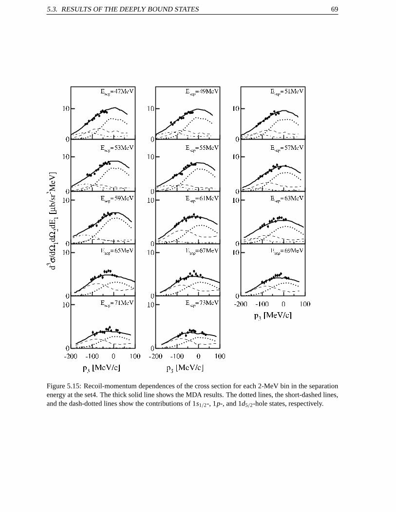
5.3. RESULTS OF THE DEEPLY BOUND STATES 69
Figure 5.15: Recoil-momentum dependences of the cross section for each2-MeV bin in the separationenergy at the set4. The thick solid line shows the MDA results. The dotted lines,the short-dashed lines,and the dash-dotted lines show the contributions of 1s1/2-, 1p-, and 1d5/2-hole states, respectively.

70 CHAPTER 5. RESULT
Figure 5.16: Recoil-momentum dependences of the analyzing power for each 2-MeV bin in the separa-tion energy at the set4. TheAy data was not included in the MDA. The dotted lines, the short-dashedlines, and the dash-dotted lines show the contributions of 1s1/2-, 1p-, and 1d5/2-hole states, respec-tively.

5.3. RESULTS OF THE DEEPLY BOUND STATES 71
Figure 5.17: Recoil-momentum dependences of the cross section for each2-MeV bin in the separationenergy at the set5. The thick solid line shows the MDA results. The dotted lines,the short-dashed lines,and the dash-dotted lines show the contributions of 1s1/2-, 1p-, and 1d5/2-hole states, respectively.

72 CHAPTER 5. RESULT
Figure 5.18: Recoil-momentum dependences of the analyzing power for each 2-MeV bin in the separa-tion energy at the set5. TheAy data was not included in the MDA. The dotted lines, the short-dashedlines, and the dash-dotted lines show the contributions of 1s1/2-, 1p-, and 1d5/2-hole states, respec-tively.
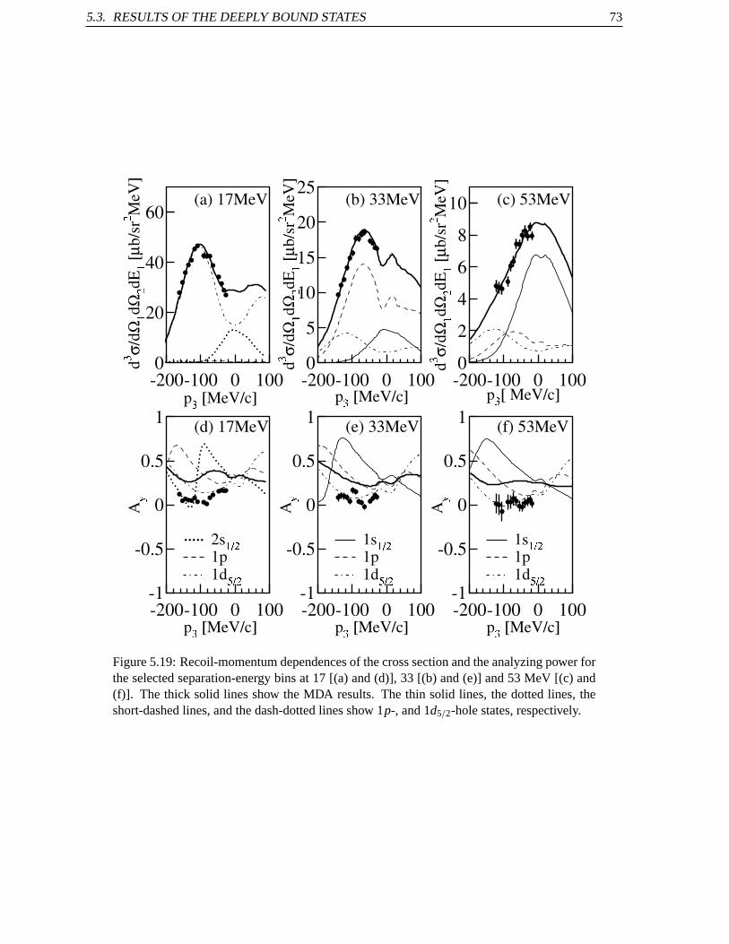
5.3. RESULTS OF THE DEEPLY BOUND STATES 73
Figure 5.19: Recoil-momentum dependences of the cross section and the analyzing power forthe selected separation-energy bins at 17 [(a) and (d)], 33 [(b) and(e)] and 53 MeV [(c) and(f)]. The thick solid lines show the MDA results. The thin solid lines, the dotted lines, theshort-dashed lines, and the dash-dotted lines show 1p-, and 1d5/2-hole states, respectively.

74 CHAPTER 5. RESULT
Figure 5.20: Strength distributions obtained in the separation-energy region of 12–84 MeV. The solidlines are shown to guide the eyes. The vertical dotted line at 24 MeV in (a) shows the border wherethe s-hole state contribution was divided into the contribution of the 2s1/2-hole state and that of the1s1/2-hole state.

5.3. RESULTS OF THE DEEPLY BOUND STATES 75
Figure 5.21: Strength distributions for the hole states of the (a) 1s1/2, (b) 1p, (c) 2s1/2, and (d) 1d5/2
orbitals in the separation energy region of 12–84 MeV. The solid lines and the dash-dotted lines inthe figures for the 1s1/2-, 1p- and 1d5/2-hole states show the fitted curves and the fitted asymmetricLorentzian functions, respectively. The short-dashed lines show the estimated contribution of the four-body background.

76 CHAPTER 5. RESULT

Chapter 6
Discussion
6.1 DWIA calculation
For the first two peaks at 8.3 and 10.9 MeV in the separation energy spectra, the cross sections and ana-
lyzing powers are reproduced by the DWIA calculation qualitatively well, which are shown in Figs. 5.7
and 5.8, and the peaks seem involve scarcely any background. Nevertheless the spectroscopic factor for
the 1d3/2-hole state exceeds 100% of the 2J + 1 value, and that of the 2s1/2-hole state is much larger
than the value from (e, e′p) and (d,3He) reactions as shown in Table 5.1. The validity of the DWIA
calculation is discussed for the hole states of the valence orbitals.
First, the results of DWIA calculation with other distorting potentials are displayed in Figs. 6.1 and
6.2. For the 1d3/2, 2s1/2, and 1f7/2-hole states, the other parameter sets of Cooperet al. [77] and
parameter sets of Hamaet al. [91] were used for the distorting potential. The used potentials are listed
in Table 6.1. The strengths of the 1d3/2-hole state were obtained by fitting to the experimental data. The
strengths of the 2s1/2 and 1f7/2-hole states were obtained by the MDA for the peak of 10.9 MeV, in the
same way in the previous chapter. The only contribution of 2s1/2-hole state are displayed in Fig. 6.2 for
simplicity.
The calculations by Plane Wave Impulse Approximation (PWIA) are also displayed by thick solid
Table 6.1: Global optical potentials used for the distortion in the DWIA calculation.
Potential Data for fit Num. of parameters ReferenceEDAD1 12C, 16O, 40Ca,90Zr, 208Pb(p, p) 20-1040 MeV 106 [77]EDAD2 12C, 16O, 40Ca,90Zr, 208Pb(p, p) 20-1040 MeV 154 [77]EDAD3 12C, 16O, 40Ca,90Zr, 208Pb(p, p) 20-1040 MeV 176 [77]EDAICA 40Ca(p, p) 20-1040 MeV 70 [77]DP1 40Ca,48Ca,56Fe,60Ni, 90Zr, 208Pb(p, p) 65-1040 MeV 80 [91]DP2 40Ca,48Ca,56Fe,60Ni, 90Zr, 208Pb(p, p) 65-1040 MeV 84 [91]
77

78 CHAPTER 6. DISCUSSION
Figure 6.1: DWIA calculations of the40Ca(p,2p) reaction for the 1d3/2-hole statewith different optical potentials. The parameter sets of Cooperet al. (EDAD2,EDAD3, EDAICA) [77] and of Hamaet al. (DP1, DP2) [91] were used for thedistorting potential. The strengths of the 1d3/2-hole state were obtained by fitting tothe experimental data. The thick solid line indicates the PWIA calculation withoutnormalization for the cross section.
Figure 6.2: DWIA calculations of the40Ca(p,2p) reaction for the 2s1/2-hole state at10.9 MeV with different optical potentials. The used optical potentials were sameas those for the 1s3/2-hole state in Fig. 6.1. The strength of the 2s1/2-hole statewas determined by the MDA for the peak. The only contribution of 2s1/2-hole stateare displayed for simplicity. The thick solid line indicates the PWIA calculationnormalized with a factor of 0.4 for the cross section.
lines in Figs. 6.1 and 6.2 to investigate the contribution of the distortion. The PWIAcalculations were
calculated with spectroscopic factors of 1 for the 1d3/2 and 2s1/2-hole states, and the cross section for
the 2s1/2-hole state is normalized by factor of 0.4 for the display in Fig 6.2. As was shown in Ref. [44],

6.1. DWIA CALCULATION 79
Figure 6.3: Spectroscopic factors obtainedwith the different distorting potentials for the1d3/2-, 2s1/2-, and 1f7/2-hole states.
Figure 6.4: Correlation between the spectro-scopic factors for the 1d3/2-hole state and thestrength of the spin–orbit term for the boundstate.
the shape of the analyzing power for a hole state is due to the spin–orbit part of the optical potential for
an orbital withL = 0 and to both the spin–orbit part and the effective polarization (Maris effect) for a
L , 0 orbital. Comparing these DWIA and PWIA calculations, it is confirmed that thedistortion play an
important role to reproduce the shapes of the cross section and analyzingpower not only quantitatively
but also qualitatively. The qualitative reproduction of the cross section and analyzing power show that
the DWIA works well to reproduce the data for the 392 MeV proton. It is found that the cross sections
of the DWIA calculation are diminished to about 20–30% of the PWIA values. Although these ratios
are larger than that for a heavy target such as208Pb, which is less than 5% [44], the distortion must
greatly contribute to determine absolute values of cross section.
All the results of DWIA calculation with other potentials reproduced the data qualitatively as well as
the result with EDAD1 used in the previous chapter. The shapes of the cross section and analyzing power
for the used distorting potentials are almost indistinguishable. The obtained spectroscopic factors for
the respective potentials are shown in Fig 6.3. Although there are some differences between the values,
all of them are much larger than the results from the (e, e′p) and (d,3He) reactions. There are hardly
differences on the reproduction between the potentials qualitatively and quantitatively.
Second, the sensitivity of the spectroscopic factors to various bound state parameters in the DWIA
calculation are discussed. The recoil-momentum distribution of the cross section and analyzing power
with different values for the radius parameter of the Woods-Saxon potential forthe 1d3/2- and 2s1/2-hole
states are displayed in Fig. 6.5 and 6.6. Their shapes gradually change bythe radius parameter. The
relation between the obtained spectroscopic factors and the radius parameter is shown in Fig. 6.7. A
change of 0.01 fm in the radius will change the spectroscopic factors by about 3, 2, and 5% for the
1d3/2-, 2s1/2-, and 1f7/2-hole states respectively, relative to the values with 1.30 fm by Elton and Swift.
A change of the diffuseness parameter doesn’t change the shape of the cross section andanalyzing power
as much as the radius, and the change of 0.01 fm will change the spectroscopic factors by about 1% for
all of the 1d3/2-, 2s1/2-, and 1f7/2-hole states relative to the values with 0.60 fm by Elton and Swift The

80 CHAPTER 6. DISCUSSION
Figure 6.5: DWIA calculations of the40Ca(p,2p) reaction for the 1d3/2-hole statewith the different radius parameters of the Woods-Saxon potential. The strengthsof the 1d3/2-hole state were obtained by fitting to the experimental data.
relation between the obtained spectroscopic factors and the diffuseness is shown in Fig. 6.8. For the
1d3/2-hole state, the spectroscopic factor gradually changes about 2% by 1 MeV of the strength of the
spin-orbit term, which is shown in Fig.6.4.
Third, the spectroscopic factors are discussed under the condition thatthe DWIA calculation is
performed with a bound-state-parameter set by Krameret al. For the (e, e′p) and (d,3He) reactions,
Krameret al. performed their analysis with the common bound state wave function and obtained con-
sistent spectroscopic factors [52]. Their parameters were determined by the analysis for the (e, e′p)
reaction because the (e, e′p) reaction is sensitive to the whole of the bound state wave function. The
DWIA calculation was performed with the bound state parameters from the papers [79, 52] by Krameret
al., and the spectroscopic factors from the (p,2p) reaction were obtained for the present experiment. The
distorting potential of EDAD1 was used for the (p,2p) reaction. Figure. 6.9 show the difference of the
spectroscopic factors between from the (p,2p) reaction ((A) and (B)) and from the (e, e′p) reaction (C)
in the reference [52]. The analysis by Krameret al. includes the nonlocality corrections in the bound
state wave function and in the reaction. For the (p,2p) reaction, the nonlocality corrections were not
included in the case (A) but included in the case (B). The nonlocality corrections were applied with a
nonlocality range ofβ = 0.85 fm by Perey and Buck [92]. Comparing this two cases of (A) and (B),
the nonlocality corrections reduce the spectroscopic factors. The differences between the cases of the
(p,2p) and (e, e′p) reactions ((B) and (C)) are about 20% or more, and they are due to anelement ex-
cept the bound state wave function, that is, the distortion potential, the framework of the calculation,
and so forth. Therefore, the differences of the spectroscopic factors between from the (p,2p) in the
present work and from the (e, e′p) reactions are due not only to the bound-state parameters but also to
the treatment of the distortion in the (p,2p) reaction.
The radius and diffuseness parameters by Elton and Swift in Table 4.1 are common for all orbitalsin

6.1. DWIA CALCULATION 81
Figure 6.6: DWIA calculations of the40Ca(p,2p) reaction for the 2s1/2-hole statewith the different radius parameters of the Woods-Saxon potential. The strength ofthe 2s1/2-hole state was determined by the MDA for the peak. The only contribu-tion of 2s1/2-hole state are displayed for simplicity.
40Ca, and are not optimized for each orbital. These values are not greatly different from the values by
Krameret al., and the difference of the radius and the diffuseness parameters from those by Krameret
al. will make the difference of the cross section by 5% or less. The difference of the spin–orbit strength
makes 11% difference of the cross section.
For not only the valence orbitals but also the deeply bound orbitals, the DWIA calculation was per-
formed with the nonlocality corrections, and the spectroscopic factors obtained by fitting and the MDA
was shown in Fig. 6.10 with the result obtained in previous chapter. The nonlocality corrections decrease
the spectroscopic factors for all of the orbitals almost uniformly.
It should be noted that the values of the spectroscopic factors often have different values for the mea-
surement angles and the used distortion potentials for the (p,2p) reaction even at the proton-injection
energy of 200 MeV, where many (p,2p) experiments have vigorously been performed [40, 44, 84, 85].
It is seen in Table 5.1 for the valence orbitals in40Ca that the differences of the spectroscopic factors
between the measured angles have not been settled yet and the differences of them by about 2 times are
found in papers.
The aim of this work is to investigate the spectroscopic factors for the deeplybound orbitals. In order
to discuss them in spite of the unsettled matters of the DWIA calculation, the spectroscopic factors were
normalized by using the value from the (e, e′p) reaction. Since there was no way to optimize bound-state
parameters for the overlapped deeply bound orbitals, the result with the common bound state parameters
by Elton and Swift was used in the following. The relative ratio of the spectroscopic factor for the 1d3/2
orbital from the (e, e′p) reaction by Krameret al. to that obtained in the present analysis was 0.53.
In the following sections, the spectroscopic factors are normalized by the factor of 0.53, which are
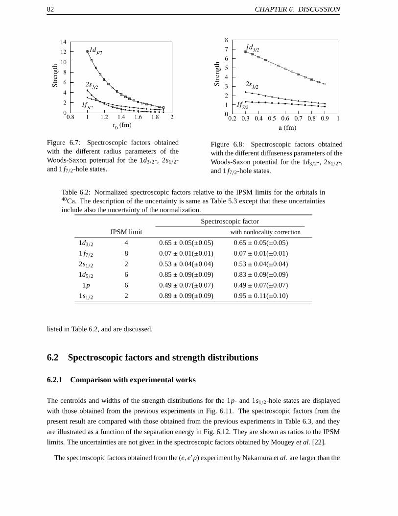
82 CHAPTER 6. DISCUSSION
Figure 6.7: Spectroscopic factors obtainedwith the different radius parameters of theWoods-Saxon potential for the 1d3/2-, 2s1/2-and 1f7/2-hole states.
Figure 6.8: Spectroscopic factors obtainedwith the different diffuseness parameters of theWoods-Saxon potential for the 1d3/2-, 2s1/2-,and 1f7/2-hole states.
Table 6.2: Normalized spectroscopic factors relative to the IPSM limits for the orbitals in40Ca. The description of the uncertainty is same as Table 5.3 except that theseuncertaintiesinclude also the uncertainty of the normalization.
Spectroscopic factor
IPSM limit with nonlocality correction
1d3/2 4 0.65± 0.05(±0.05) 0.65± 0.05(±0.05)
1 f7/2 8 0.07± 0.01(±0.01) 0.07± 0.01(±0.01)
2s1/2 2 0.53± 0.04(±0.04) 0.53± 0.04(±0.04)
1d5/2 6 0.85± 0.09(±0.09) 0.83± 0.09(±0.09)
1p 6 0.49± 0.07(±0.07) 0.49± 0.07(±0.07)
1s1/2 2 0.89± 0.09(±0.09) 0.95± 0.11(±0.10)
listed in Table 6.2, and are discussed.
6.2 Spectroscopic factors and strength distributions
6.2.1 Comparison with experimental works
The centroids and widths of the strength distributions for the 1p- and 1s1/2-hole states are displayed
with those obtained from the previous experiments in Fig. 6.11. The spectroscopic factors from the
present result are compared with those obtained from the previous experiments in Table 6.3, and they
are illustrated as a function of the separation energy in Fig. 6.12. They areshown as ratios to the IPSM
limits. The uncertainties are not given in the spectroscopic factors obtainedby Mougeyet al. [22].
The spectroscopic factors obtained from the (e, e′p) experiment by Nakamuraet al. are larger than the

6.2. SPECTROSCOPIC FACTORS AND STRENGTH DISTRIBUTIONS 83
Figure 6.9: Spectroscopic factors obtained with the common bound state parame-ters by Krameret al. [79, 52] for the 1d3/2- and 2s1/2-hole states. The spectroscopicfactors of (A) and (B) were obtained by the present analysis, and thatof (C) is fromRef. [52]. The nonlocality correction was included in (B) and (C) with a nonlocalityrange ofβ = 0.85 fm by Perey and Buck [92].
sum-rule limits except for the 1d5/2 orbital [24]. Their large spectroscopic factors for the 1p and 1s1/2
orbitals possibly suggest the inclusion of the continuum background in the higher-separation-energy
region. The spectroscopic factors of 0.65 and 0.75 obtained by Mougeyet al. [22] for the 2s1/2 and
1s1/2 orbitals are as low as the present results of 0.53 and 0.89, whereas the spectroscopic factor of
0.95 for the 1p orbital is much larger than the present result of 0.49. The centroid energy of 41 MeV
obtained by Mougeyet al. for the 1p orbital is much higher than the present result of 29.6 MeV as seen in
Table 5.2. As can be seen in Fig. 6.12, both the centroid energies of the 1p and 1s orbitals by Mougeyet
al. are higher than those from the present result. The larger spectroscopic factor and the higher centroid
energy for the 1p orbital can possibly be explained by inclusion of the continuum background in the
1p-hole strengths in the higher-separation-energy region or by an insufficient separation of the 1p- and
1s-hole states. It is also possible that the extremely high centroid energy of 77MeV for the 1s1/2-hole
state reported by Amaldiet al. [25] is due to the continuum background at higher separation energy.
The centroid energies and widths of the 1s1/2 and 1p-hole states obtained in the present results are close
to the results from the (p,2p) experiment at PNPI [53].
The present analysis also depends on the background treatment. The spectroscopic factors obtained
without background subtraction for the 1s1/2, 1p, and 1d5/2 orbitals are 1.5–2.0 times larger than those
subtracted backgrounds, as seen in Tables 5.3 and 5.4. This indicates that the spectroscopic factors are
greatly affected by the background estimation.
The background from the four-body final states in the high-missing-energy region in the12C(e, e′p)
reaction was investigated by Fissumet al. at JLab [93]. The measured separation-energy spectra were
compared with calculation of the (e, e′pp) and (e, e′pn) reactions included meson-exchange currents,
isobar currents, central short-range correlations, and tensor medium-range correlations. However, the
calculated cross section was smaller than the measured cross section by about 50% and did not clarify
the total background components.

84 CHAPTER 6. DISCUSSION
Figure 6.10: Spectroscopic factors relative to the IPSM limits for the orbitals in40Ca as a function ofthe separation energy. The solid line and dashed line are shown to guide theeyes.
The contribution of the rescattering processes was studied by Cowleyet al. [88]. It is remarkable that
the calculated rescattering processes well reproduced the experimentalcoincidence spectra especially
in the kinematical region in which the quasi-free events were hardly expected. The rescattering process
cannot be ignored in some kinematical regions in the coincidence measurement.
Although the background components are still controversial, in the present study, we used the four-
body phase space as the background-shape model, taking account ofthe four-body and rescattering
processes. To compensate for the inadequacy of the model, the uncertainties in the deduced observables
were estimated to include the model uncertainties, as previously mentioned.
A large reduction in single-particle strength has also been observed for the strongly bound valence
neutrons near the Fermi surface in proton-rich unstable nuclei [94, 95]. This reduction has been sug-
gested to be due to the strongp–n interactions [96]. Although the nucleons in the 1p and 1s1/2 orbitals
in 40Ca are also strongly bound, these orbitals are far below the Fermi surface. Therefore, the mech-
anisms for reducing the spectroscopic factors for the 1p and 1s1/2 orbitals in 40Ca is expected to be
different. We need further experimental study on the spectroscopic factorsin other nuclei to clarify the
NN correlations that contribute to the reduction of the spectroscopic factors for deeply bound orbitals.
6.2.2 Comparison with theoretical works
The spectroscopic factors from the present result are compared with those from theoretical studies in
Table 6.4, and they are illustrated as a function of the separation energy in Fig. 6.13. They are shown as
ratios to the IPSM limits.
The calculations reported by Fabrociniet al. [20] and by Biscontiet al. [21] used state dependent

6.2. SPECTROSCOPIC FACTORS AND STRENGTH DISTRIBUTIONS 85
Figure 6.11: Centroids (symbols) and FWHM widths (solid lines) of the strengthdistributions for the 1p- and 1s1/2-hole states with those obtained from the previousexperiments, from Table 5.2.
correlations with central and tensor components, so-calledf6 correlation. Although Fabrociniet al.
ignored Coulomb interaction in the mean field potential and used thels coupling scheme of the single-
particle wave function basis, Biscontiet al. followed the calculation in Ref. [20] by Fabrociniet al.,
and considered the presence of the antiparallel spin terms and distinguished between proton and neutron
contributions in thej j coupling scheme for sake of completeness. Both calculations suggested that the
spectroscopic factor decreases as the binding energy increases, ascan be seen in Fig. 6.13. This is con-
trary to the prediction by the nuclear matter calculation by Benharet al.[13]. Furthermore, Biscontiet
al. insisted from the results of12C, 16O, 40Ca, 48Ca, and208Pb that the spectroscopic factors increase
when the principle quantum numbern and thel j values increase. Although the values predicted by
Biscontiet al. show a rather moderate reduction, the quantitative difference between these calculations
was not discussed. The role played by the various correlations have been unclear.
The spectroscopic factors of 0.86 and 0.87 for the 2s1/2 orbital predicted by Fabrociniet al. [20] and
Biscontiet al. [21] considerably exceed the present result of 0.53. This discrepancy could be explained
by surface effects, which are not taken into account in their calculations. It is known theoretically that
the surface effects reduce the spectroscopic factors for the orbitals near the Fermi level.
Though the spectroscopic factor of 0.85 for the 1d5/2 orbital is consistent with the values predicted
by Fabrociniet al. and by Biscontiet al., those for the 1s1/2 and 1p orbitals show a different tendency
from the predictions. The spectroscopic factor obtained for the 1s1/2 orbital is as small as that for the
1d5/2 orbital, and they are about 90% of the 2J + 1 value; they indicate small suppression as predicted
by Bisconti et al. On the other hand, the spectroscopic factor of 0.49 for the 1p orbital is largely
suppressed and is smaller than the predicted value of 0.58 by Fabrociniet al. The large reduction of the
spectroscopic factor for the 1p orbital indicates a strong influence ofNN correlations in the inner core

86 CHAPTER 6. DISCUSSION
Table 6.3: Spectroscopic factors relative to the IPSM limits for the orbitals in40Ca obtained fromprevious experiments. For the present result, the description of the uncertainty is same as Table 6.2.
IPSM limit Present work Mougeyet al. [22] a Nakamuraet al.[24] b
2s1/2 2 0.53± 0.04(±0.04) 0.65 1.0± 0.1
1d 10 0.77
1d3/2 4 0.65± 0.05(±0.05) 1.1± 0.4
1d5/2 6 0.85± 0.09(±0.09) 0.78± 0.27
1p 6 0.49± 0.07(±0.07) 0.95 1.70± 0.15
1s1/2 2 0.89± 0.09(±0.09) 0.75 2.60± 0.15 (A)
1.9± 0.1 (B)
aThe uncertainties were not given for the spectroscopic factors by Mougeyet al..bTwo results ((A) and (B)) were presented for 1s1/2 orbital.
Table 6.4: Spectroscopic factors relative to the IPSM limits for the orbitals in40Ca obtained fromtheoretical studies. For the present result, the description of the uncertainty is same as Table 6.2.
IPSM limit Present work Fabrociniet al. [20] Biscontiet al. [21]
2s1/2 2 0.53± 0.04(±0.04) 0.86 0.87
1d 10 0.87
1d3/2 4 0.65± 0.05(±0.05) 0.85
1d5/2 6 0.85± 0.09(±0.09) 0.86
1p 6 0.49± 0.07(±0.07) 0.58
1p1/2 2 0.81
1p3/2 4 0.82
1s1/2 2 0.89± 0.09(±0.09) 0.55 0.78
far below the Fermi surface. On the other hand, the small quenching for the 1s1/2 orbital may support
moderate effect byNN correlations.
The spectroscopic factors for the 1d5/2, 1p and 1s1/2 don’t show monotonous decrease or increase
with respect to binding energy as predicted. Present result possibly suggests other dependence of theNN
correlations,e.g., l dependence, and a clue to disentangle the role played by the correlations.Therefore,
it is interesting to investigate the spectroscopic factor for the 1p orbital in detail. The spectroscopic
factor for the 1p orbital was obtained on the assumption that the relative strengths for the 1p1/2 and
1p3/2-hole states are in the ratio of 2:4. It is significant to deduce the spectroscopic factors for the 1p1/2
and 1p3/2-hole states separately to obtain further information on the reduction of the spectroscopic factor
for the deeply bound orbitals.

6.3. PERSPECTIVES 87
Figure 6.12: Spectroscopic factors relative to the IPSM limits for the orbitals in40Ca as a function ofthe separation energy with the result by Mougeyet al. The solid line and dashed line are shown to guidethe eyes.
6.3 Perspectives
The 1p1/2- and 1p3/2-hole states could not be separated in the present study because the DWIA cal-
culation of the analyzing power was not fully reliable. It is important to be ableto separate the hole
states of the 1p1/2 and 1p3/2 orbitals, that is, the hole states of thej> and j< orbitals, by use of the
analyzing power data, to obtain further information on the deeply bound orbitals and to understandNN
correlations in atomic nuclei.
In the (~p,2p) reaction experiment following the present work at RCNP with a polarized proton beam
at 200 MeV, theAy data was reproduced by the DWIA calculation better than that in the present
work [97], and it encourages us to separate the hole states of thej> and j< orbitals. Since the mea-
surement was performed under the symmetric angle condition for ejected protons, the symmetric angle
condition seems to be advantageous to theAy measurement. We have not understood why the DWIA
calculation reproduced theAy data in the lower injection-energy experiment and have to get an reason-
able understanding on its reason to use theAy data for the MDA. Progress in the theoretical models that
can explain the reduction of the analyzing power is also expected. TheAy measurement at 200 MeV
under the symmetric angle condition is attractive to separate the 1p1/2- and 1p3/2-hole states. though
background contribution might interfere theAy for deeply bound orbitals.
Bisconti suggested that short-range correlations have small effects on the density distributions in
nuclei and that the tensor part of the correlation is important in the calculationof the occupation proba-
bilities. To understand the detail ofNN correlations and include them in the description of the nuclear
structure, we should investigate roles and influence ofNN correlations. For this purpose, we need sys-
tematic information on the spectroscopic factors in various nuclei for the orbitals far below the Fermi

88 CHAPTER 6. DISCUSSION
Figure 6.13: Spectroscopic factors relative to the IPSM limits for the orbitals in40Ca as a function of theseparation energy with the predictions by Fabrociniet al. [20] and Biscontiet al. [21]. For the separationenergies of the predictions, the values of the present result are used since no predicted values are in theirpapers. The separation energies for the 1p1/2 and 1p3/2 orbitals are plotted deviating±2 MeV from29.6 MeV respectively. The solid line (present result), dashed line (Fabrocini et al.), and dash-dottedline (Biscontiet al.) are shown to guide the eyes.
surface where the surface effects are negligible.

Chapter 7
Summary
A 40Ca(~p,2p) experiment was performed with a 392-MeV polarized proton beam to measure the recoil-
momentum distributions of the cross section and the analyzing power in the separation-energy region of
0–89 MeV.
Although a hump structure is seen around 30 MeV in the measured separationenergy spectra, no peak
or hump cannot be seen over 40 MeV, where 1s-hole state is expected to be seen.
Two prominent peaks were observed at 8.3 and 10.9 MeV in the separationenergy spectra, and their
recoil-momentum distributions of the cross section show characteristic behavior for a hole state of a
single-particle orbital withL , 0 andL = 0, respectively. It was confirmed that the DWIA calculation
reproduces the dependence of the recoil momentum on the measured cross section and analyzing power
qualitatively well. However, the obtained spectroscopic factors for the 1d3/2 and 2s1/2 are larger than
those from the (e, e′p) and (d,3He) reactions, and the DWIA calculation systematically overestimates
the analyzing power for 1d3/2 and 2s1/2-hole states. The differences of the spectroscopic factors of the
valence orbitals between from the (p,2p) in the present work and from the (e, e′p) reactions are due not
only to the bound-state parameters but also to the treatment of the distortion in the(p,2p) reaction. It is
found that there are some uncertainties in the absolute values of the cross section and analyzing power
from the DWIA calculation in this experimental condition.
The strength distributions for the deep-hole states were obtained by the MDAfor each 2-MeV bin in
the separation energy and were successfully separated from the continuum background by subtraction
of a four-body background. The centroid energies and widths of the distributions were deduced to be
29.6± 0.6 and 48.4± 0.6 MeV for the 1p and 1s1/2-hole states, respectively. The hump of the 1p-hole
state around 30 MeV is consistent with the hump structure in separation energy spectra.
Taking the uncertainty of the DWIA calculation into the consideration, the spectroscopic factors
were normalized by using the value for the 1d3/2 orbital from the (e, e′p) reaction and discussed. The
normalized spectroscopic factors for the 1p and 1s1/2 orbitals were obtained as 49± 7% and 89± 9%
of the IPSM limits, respectively, and it is indicated that the spectroscopic factors for the deeply bound
orbitals are reduced owing to theNN correlations. Further development of the DWIA calculation of the
89

90 CHAPTER 7. SUMMARY
analyzing power is expected to separate the hole states of the 1p1/2 and 1p3/2 orbitals and clarify the
influence of theNN correlations on the spectroscopic factors.
Acknowledgements
I would like to express my gratitude to Professor H. Sakaguchi, who was my supervisor at the graduate
course in Kyoto University. He suggested the study of deep hole states in the medium-mass region by
(p,2p) reaction and have patiently been discussed the subject on physics with me.I have continuously
learned experimental technique from him.
I would like to thank Professor T. Kawabata for his helpful discussion and guidance on the present
work. I appreciate his critical advice on a draft of a paper.
I acknowledge Professor M. Yosoi, who is kind enough to provide his analysis software and to give
the detail of making the MWPCs. As he is one of the experimentalists who have a detailed knowledge
of an experiment with the Grand Raiden spectrometer, I have gotten lots of advices from him not only
in the experiments but also in the analysis of the data.
I am deeply grateful to Professor T. Noro, from whom I have learnedmuch of (p,2p) experiment. He
gave me chances to join the experiments at the Petersburg Nuclear Physics Institute (PNPI), Gatchina,
Russia. We started the study of deep hole states by (p,2p) reaction since these experiments.
I would like to thank Professor T. Nagae for his thoughtful suggestions for this thesis.
I gratefully thank the scientific and technical staff and cyclotron crew at RCNP, especially Professor
K. Hatanaka and Dr. S. Ninomiya, for their support for providing a stablebeam during the experiment
and for the beam-time management.
I would address my thank to Dr. H. Takeda, who had developed the RDTM module and supported its
operation during the beamtime. I am grateful to Dr. M. Itoh for his hard workin the preparation and
in the beamtime. I am thankful to Dr. M. Uchida and Dr. H. P. Yoshida for theirgreat contribution to
the experiment, especially to the data acquisition. I wish to thank Dr. S. Terashima, Mr. S. Kishi, and
Dr. J. Zenihiro, who worked in whole of the experiment and took much of midnight shifts.
I would like to thank Professor T. Wakasa for his support and advices on a draft of a paper.
I would like to thank all other members of the RCNP-E168/217 experiments; Mr. S. Asaji, Dr. K. Fu-
jita, Mr. Y. Hagihara, Dr. T. Ishida, Professor Y. Sakemi, Dr. Y. Shimizu, Dr. Y. Tameshige, and
Mr. T. Yonemura for their great contributions.
91

92 CHAPTER 7. SUMMARY
I spent 7 years as a member of the experimental nuclear hadronic physics(NH) group at Kyoto
University. I would like to express many thanks Professor K. Imai for devoted direction. I would like to
thank Dr. T. Murakami, from whom I learned a lot of things on physics. I also thank all members of the
group, especially friendly coworkers, Dr. M. Kitaguchi and Dr. M. Miyabe.
I would like to thank Professor. A. Ozawa, Professor. H. Okamura, and Professor. A. Tamii for their
support and giving me chances to continue the research on nuclear physics at University of Tsukuba and
at RCNP, Osaka University.
I would like to express my appreciation to my parents, who have supported and encouraged me. I
also thank Dr. K. Yasuda, who is a biologist and one of my relatives. She gave some advice and cheered
me up.
Finally, I thank my wife Sachiko for her patience and encouragement during all these years.

Appendix A
Phase space calculation
A.1 Introduction
The (p,3p) and (p,2pn) reactions are possible components of the background in the (p,2p) reaction,
while the dynamical aspects in the (p,3p) and (p,2pn) reactions are unclear. In order to estimate the
contribution of those reactions in the (p,2p) reaction measurement without the dynamical details of the
(p,3p) and (p,2pn) reactions, the phase space for the 4 particle final state was calculated. Phase space
describes a kinematical aspect of the process. In this chapter, the four-body phase space is derived from
its definition.
As the DWIA calculation in the present study employs the noninvariant form, the noninvariant phase
space is employed here. The momentumpj and energyE j of the j-th particle satisfy the following
relation
E2j − p2
j = m2j , (A.1)
wherem j is the mass of the j-th particle. As is defined in Werbrouck’s textbook [98], the probability
dPn of a n-particle final state with a total momentumP and total energyE is defined as
d3nPn = d3nRnH . (A.2)
whereH is the square of the noninvariant matrix element for the process and contains the dynamical
aspects of the process, andRn is pure kinematical and the Lorentz noninvariant phase space defined by
d3nRn =
n∏
j=1
d3pj
δ3(
n∑
j=1
pj − P)
δ(
n∑
j=1
E j − E)
. (A.3)
A.2 Phase space for four-particle final state
The processes that we take account of are the40Ca(p,3p)38Ar and 40Ca(p,2pn)38K reactions. As the
final states have the configuration of 3p+38Ar or of 2p+ n+38K, respectively, the four-body phase space
93
94 APPENDIX A. PHASE SPACE CALCULATION
R4 is discussed here. The calculation employs the condition that the two protons inthe final states are
detected by GR and LAS but the other particles in the final states are not detected, as is same as the
experiment.
Let particles 1 and 2 correspond to protons detected by GR and LAS. Theparticles 3 and 4 are the
combination ofp+38Ar or n+38K. The phase space for the four-body final states is given from Eq. (A.3)
as
d4·3R4 =
4∏
j=1
d3pj
δ3(
4∑
j=1
pj − P)
δ(
4∑
j=1
E j − E)
. (A.4)
From Eq. (A.4), we have the four-body phase space in the integral form
R4(
E, P)
=
∫
d3p1 d3p2 d3p3 d3p4δ3(
p1 + p2 + p3 + p4 − P)
δ(
E1 + E2 + E3 + E4 − E)
=
∫
d3p1 d3p2
∫
d3p3d3p4δ3(
p3 + p4 − P′)
δ(
E3 + E4 − E′)
(A.5)
whereE′ andP′ are defined byE′ = E −E1−E2 andP′ = P− p1− p2, respectively. The last integral in
Eq. (A.5) corresponds to the two-body phase spaceR2(
E′, P′)
with total momentumP′ and total energy
E′.
R2(
E′, P′)
=
∫
d3p3d3p4δ3(
p3 + p4 − P′)
δ(
E3 + E4 − E′)
(A.6)
Therefore, we have
R4(
E, P)
=
∫
d3p1 d3p2 R2(
E′, P′)
. (A.7)
Under the condition that only two protons in the final states are detected, the state of the rest parti-
cles is indefinite. The 4 particle final states could contribute in the separation energy spectrum of the40Ca(p,2p)39K reaction. Excluded the reactionQ-value, the separation energy calculated from the en-
ergies of the injected and detected protons corresponds to the excitation energy of the residual nucleus
in the 3 particle final states, while it corresponds to the effective mass of the particles 3 and 4 in the 4
particle final states. The effective massM34 of the particles 3 and 4 is defined by
M234 =
(
E3 + E4)2 − (
p3 + p4)2. (A.8)
In order to estimate the contribution of the 4 particle final states in the separationenergy spectrum of
the40Ca(p,2p)39K reaction, the mass distribution of the four-body phase space
dR4
dM34(A.9)
is needed. By using the conservation laws of momentum and energy, the effective massM34 is expressed
as
M234 =
(
E − E1 − E2)2 − (
P − p1 − p2)2
=(
M2 + m21 + m2
2 − 2EE1 + 2P · p1)2 − 2EE2 + 2E1E2 − 2P · p1 − 2p1 · p2 . (A.10)

A.3. PHASE SPACE FOR TWO-PARTICLE FINAL STATE 95
Let p j = |p j|, and differentiating Eq. (A.10) with respect top2 gives
dM34
dp2= − 1
M34
(
(
E − E1) p2
E2+ P cosθ2 − p1 cosθ12
)
. (A.11)
The use ofdE j
dp j=
p j
E jgives the other forms ofd3pj
d3pj = p2jdp jdΩ j = p jE jdE jdΩ j . (A.12)
Combining Eq. (A.7), Eq. (A.11), and Eq. (A.12) yields
R4(
E, P)
=
∫
p1E1dE1dΩ1p22dp2dΩ2 R2
(
E′, P′)
=
∫
p1E1dE1dΩ1p22dΩ2 dM34
∣
∣
∣
∣
∣
∣
dp2
dM34
∣
∣
∣
∣
∣
∣
R2(
E′, P′)
. (A.13)
Therefore, Eq. (A.9) is obtained as
dR4
dM34=
∫
dE1dΩ1dΩ2 p1E1p22
∣
∣
∣
∣
∣
∣
dp2
dM34
∣
∣
∣
∣
∣
∣
R2(
E′, P′)
. (A.14)
The phase space for the four-body final state is calculated under the condition that two protons from
a final state are detected by the GR and LAS. Therefore, the parameters of particle 1 and 2 are given by
the measurement condition. The integral range of these parameters are determined by the acceptances
of the GR and LAS.
A.3 Phase space for two-particle final state
When the parameters of the particles 1 and 2 are given, the energyE′ and momentumP’ of the rest
two-body system are determined.
At the integration of Eq. (A.6) overp4, the integration rules for aδ-function gives
R2(
E′, P′)
=
∫
d3p3 d3p4δ3(p3 + p4 − P′
)
δ(
E3 + E4 − E′)
=
∫
d3p3
[
ψ(
p4)
∣
∣
∣
∣
∣
∣
∂A∂p4
∣
∣
∣
∣
∣
∣
−1 ]
p4=p4∗. (A.15)
whereA = p4−(
P′ − p3)
. Since the solutionp4∗ of A = 0 is p4
∗ =(
P′ − p3)
and ∂A∂p4= 1,
R2(
E′, P′)
=
∫
d3p3 δ(√
p23 + m2
3 +
√
(
P′ − p3)2+ m2
4 − E′)
.
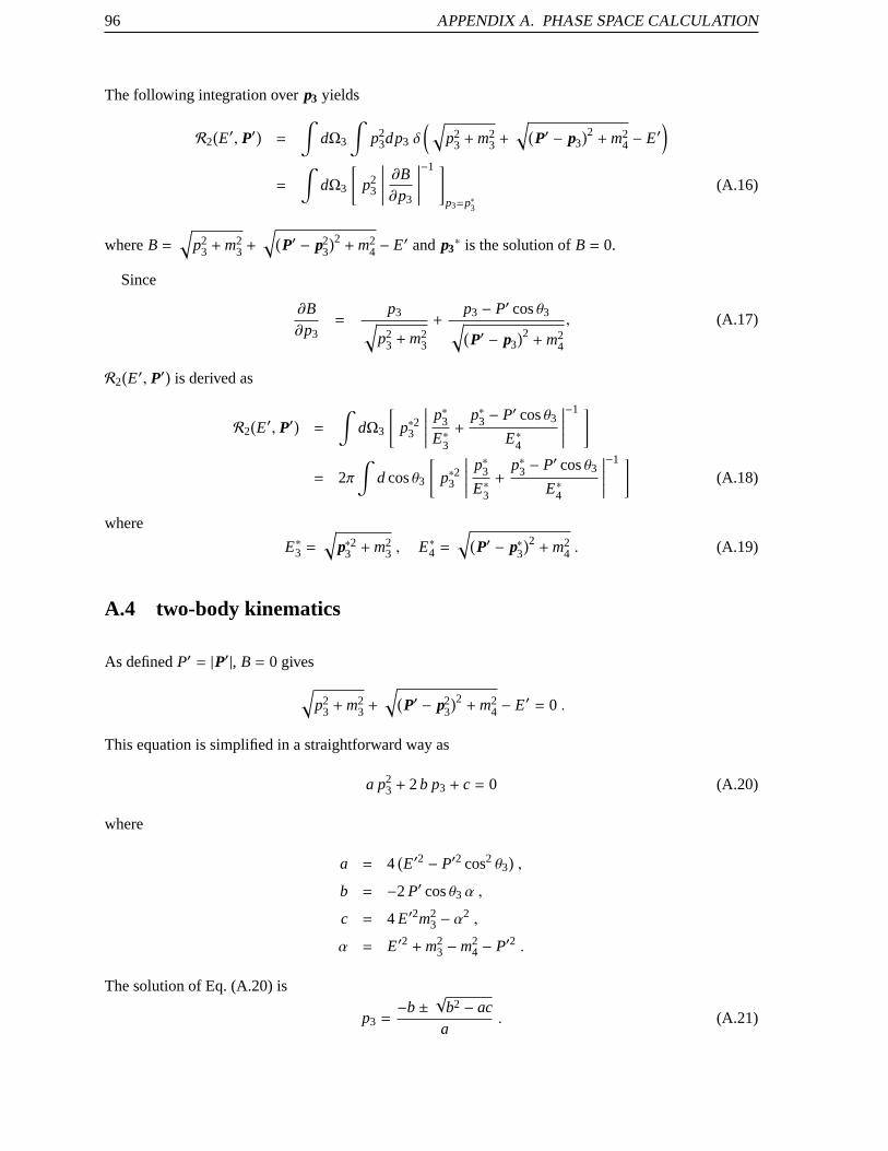
96 APPENDIX A. PHASE SPACE CALCULATION
The following integration overp3 yields
R2(
E′, P′)
=
∫
dΩ3
∫
p23dp3 δ
(√
p23 + m2
3 +
√
(
P′ − p3)2+ m2
4 − E′)
=
∫
dΩ3
[
p23
∣
∣
∣
∣
∣
∣
∂B∂p3
∣
∣
∣
∣
∣
∣
−1 ]
p3=p∗3
(A.16)
whereB =√
p23 + m2
3 +
√
(
P′ − p23
)2+ m2
4 − E′ andp3∗ is the solution ofB = 0.
Since
∂B∂p3
=p3
√
p23 + m2
3
+p3 − P′ cosθ3
√
(
P′ − p3)2+ m2
4
, (A.17)
R2(
E′, P′)
is derived as
R2(
E′, P′)
=
∫
dΩ3
[
p∗23
∣
∣
∣
∣
∣
∣
p∗3E∗3+
p∗3 − P′ cosθ3
E∗4
∣
∣
∣
∣
∣
∣
−1 ]
= 2π∫
d cosθ3
[
p∗23
∣
∣
∣
∣
∣
∣
p∗3E∗3+
p∗3 − P′ cosθ3
E∗4
∣
∣
∣
∣
∣
∣
−1 ]
(A.18)
where
E∗3 =√
p∗23 + m23 , E∗4 =
√
(
P′ − p∗3)2+ m2
4 . (A.19)
A.4 two-body kinematics
As definedP′ = |P′|, B = 0 gives
√
p23 + m2
3 +
√
(
P′ − p23
)2+ m2
4 − E′ = 0 .
This equation is simplified in a straightforward way as
a p23 + 2b p3 + c = 0 (A.20)
where
a = 4(
E′2 − P′2 cos2 θ3)
,
b = −2 P′ cosθ3α ,
c = 4 E′2m23 − α2 ,
α = E′2 + m23 − m2
4 − P′2 .
The solution of Eq. (A.20) is
p3 =−b ±
√b2 − ac
a. (A.21)

A.5. SUPPLEMENT 97
The physical solutionp∗3 of theB = 0 is thep3 solutions that are real and positive. This solution ofp∗3makes the two-body phase space of Eq. (A.18) definite, therefore, the mass distribution of the four-body
phase space of Eq. (A.14) is also given.
Here, the condition under which the physical solution exists is discussed ata different viewpoint. In
the center of mass system of the particles 3 and 4, the momentum of the particle 3 isgiven as
pc3 =
√
M234−
(
m3 + m4)2M2
34−(
m3 − m4)2
2M34. (A.22)
The relative velocitiesβc3 =
pc3
E∗3andβ = P′
E′ are defined, andγ∗3 =1
√
1−βc23
, γ = 1√1−β
. There are 3
cases depending on the relative velocities. Letθ3 be the angle between the directions ofp3 andP’. The
number of the physical solution ofp3 and the maximum of the angleθ3 are classified by 3 cases.
1. β < βc3
There is one physical solution forp3 and(
θ3)
max = 180.
2. β = βc3
There is one physical solution forp3 and(
θ3)
max = 90.
3. β > βc3
There are two physical solutions forp3 and(
θ3)
max is given as follows.
cos(
θ3)
max =
√
1−(
β∗3γ∗3
βγ
)2
(A.23)
A.5 supplement
The probability of the reaction for then-particle final statePn is defined in Lorentz invariant form as
d4nPn = d4nRnH. (A.24)
H is the square of the invariant matrix element for the process andRn is the invariant phase space defined
by
d4nRn =
n∏
j=1
d4q j δ4(
n∑
j=1
q j − Q)
n∏
j=1
δ(
q2j − m2
j)
. (A.25)
q j represents a four-momentum of the j-th particle that has an energyE j and a momentumpj,
q j =(
E j, pj)
. (A.26)
It satisfies the following relation
q2j = E2
j − p2j = m2
j . (A.27)
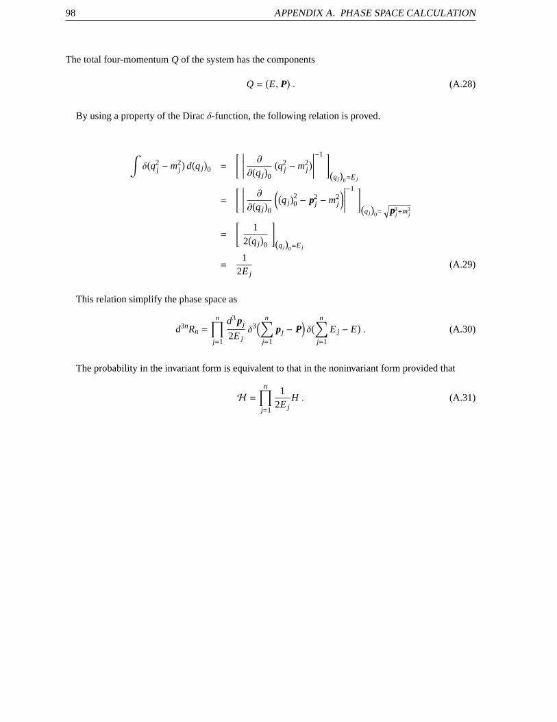
98 APPENDIX A. PHASE SPACE CALCULATION
The total four-momentumQ of the system has the components
Q =(
E, P)
. (A.28)
By using a property of the Diracδ-function, the following relation is proved.
∫
δ(
q2j − m2
j)
d(
q j)
0 =
[∣
∣
∣
∣
∣
∣
∂
∂(
q j)
0
(
q2j − m2
j)
∣
∣
∣
∣
∣
∣
−1 ]
(
q j
)
0=E j
=
[∣
∣
∣
∣
∣
∣
∂
∂(
q j)
0
(
(
q j)20 − p2
j − m2j
)
∣
∣
∣
∣
∣
∣
−1 ]
(
q j
)
0=
√
p2j+m2
j
=
[
12(
q j)
0
]
(
q j
)
0=E j
=1
2E j(A.29)
This relation simplify the phase space as
d3nRn =
n∏
j=1
d3pj
2E jδ3
(
n∑
j=1
pj − P)
δ(
n∑
j=1
E j − E)
. (A.30)
The probability in the invariant form is equivalent to that in the noninvariantform provided that
H =n
∏
j=1
12E j
H . (A.31)

Appendix B
Numerical data tablesTable B.1: Data table for the40Ca(~p,2p) reaction for the peaks at 8.3 and 10.9 MeV in the separationenergy at the set1 in Table 2.1.
Esep E1 p3dσ
dΩ1dΩ2dE1Ay
(MeV) (MeV) (MeV/c) (µb/sr2 MeV)8.3 230.0 −164.3 59.23± 0.62 0.215± 0.0158.3 234.0 −154.9 73.63± 0.70 0.244± 0.0138.3 238.0 −145.4 86.84± 0.76 0.231± 0.0128.3 246.0 −126.4 116.27± 0.86 0.202± 0.0108.3 250.0 −116.7 124.91± 0.91 0.233± 0.0108.3 254.0 −107.1 130.78± 0.92 0.209± 0.0108.3 258.0 −97.4 131.42± 0.93 0.207± 0.0108.3 266.0 −77.7 121.58± 0.90 0.154± 0.0108.3 270.0 −67.8 104.50± 0.83 0.097± 0.0118.3 274.0 −57.9 88.61± 0.78 0.086± 0.0128.3 278.0 −47.9 74.03± 0.72 0.059± 0.0148.3 286.0 −28.0 49.89± 0.41 0.130± 0.0138.3 290.0 −18.6 43.50± 0.55 0.220± 0.0208.3 294.0 −11.4 40.51± 0.55 0.353± 0.0218.3 298.0 12.0 41.09± 0.57 0.415± 0.021
10.9 230.0 −160.3 34.77± 0.48 0.002± 0.02010.9 234.0 −150.9 35.93± 1.14 0.031± 0.02010.9 238.0 −141.3 36.34± 0.50 0.015± 0.02010.9 246.0 −122.1 32.42± 0.49 −0.085± 0.02110.9 250.0 −112.4 28.14± 0.46 −0.053± 0.02310.9 254.0 −102.6 27.89± 0.47 0.062± 0.02410.9 258.0 −92.8 32.34± 0.50 0.242± 0.02210.9 266.0 −73.0 72.82± 0.75 0.432± 0.01410.9 270.0 −62.9 116.95± 0.96 0.429± 0.01110.9 274.0 −52.8 172.49± 1.20 0.409± 0.01010.9 278.0 −42.6 239.18± 1.45 0.387± 0.00810.9 286.0 −22.2 382.27± 1.43 0.326± 0.00610.9 290.0 −12.5 422.91± 2.14 0.310± 0.00810.9 294.0 6.9 437.52± 2.11 0.282± 0.00710.9 298.0 13.3 416.79± 1.98 0.263± 0.007
99

100A
PP
EN
DIX
B.
NU
ME
RIC
AL
DATA
TAB
LES
Table B.2: Data table for the40Ca(~p,2p) reaction at the set2 in Table 2.1.∆Esep= 2 MeV.
Esep E1 p3dσ
dΩ1dΩ2dE1Ay
(MeV) (MeV) (MeV/c) (µb/sr2 MeV)13.0 214.0 −169.3 19.58± 0.37 0.071± 0.02613.0 218.0 −160.6 19.07± 0.37 0.078± 0.02713.0 222.0 −151.9 19.54± 0.37 0.076± 0.02713.0 226.0 −143.1 23.07± 0.40 0.078± 0.02513.0 230.0 −134.4 31.58± 0.45 0.039± 0.02013.0 234.0 −125.6 28.20± 0.43 0.062± 0.02213.0 238.0 −116.9 27.05± 0.43 0.087± 0.02213.0 246.0 −99.3 44.81± 0.54 0.044± 0.01713.0 250.0 −90.6 36.81± 1.07 0.069± 0.01913.0 254.0 −81.9 32.90± 1.35 0.111± 0.02113.0 258.0 −73.3 32.41± 1.36 0.117± 0.02113.0 266.0 −56.5 36.02± 0.42 0.231± 0.01813.0 270.0 −48.6 32.77± 0.40 0.236± 0.01913.0 274.0 −41.4 33.86± 0.41 0.260± 0.01913.0 278.0 −35.4 35.18± 0.42 0.265± 0.01815.0 214.0 −166.1 38.10± 0.80 0.110± 0.01815.0 218.0 −157.3 46.08± 0.53 0.057± 0.01615.0 222.0 −148.5 53.07± 0.57 0.044± 0.01515.0 226.0 −139.7 56.73± 0.59 0.053± 0.01515.0 230.0 −130.9 56.41± 0.59 0.060± 0.01515.0 234.0 −122.1 63.88± 0.62 0.064± 0.01415.0 238.0 −113.2 68.06± 0.64 0.028± 0.01315.0 246.0 −95.5 56.86± 0.60 0.072± 0.01515.0 250.0 −86.7 59.41± 1.22 0.088± 0.01415.0 254.0 −77.8 60.35± 1.54 0.083± 0.01415.0 258.0 −69.1 56.77± 1.23 0.121± 0.01515.0 266.0 −52.1 48.26± 0.46 0.148± 0.01515.0 270.0 −44.1 47.33± 0.47 0.204± 0.01515.0 274.0 −36.9 44.67± 0.46 0.194± 0.01615.0 278.0 −31.1 41.20± 0.45 0.217± 0.017
Table B.2(Continued)
Esep E1 p3dσ
dΩ1dΩ2dE1Ay
(MeV) (MeV) (MeV/c) (µb/sr2 MeV)17.0 214.0 −162.9 27.93± 0.43 0.122± 0.02217.0 218.0 −154.1 32.04± 0.46 0.046± 0.02017.0 222.0 −145.2 35.90± 0.48 0.068± 0.01917.0 226.0 −136.3 39.01± 0.50 0.053± 0.01817.0 230.0 −127.5 40.84± 0.51 0.049± 0.01717.0 234.0 −118.5 45.33± 0.53 0.079± 0.01717.0 238.0 −109.6 46.61± 0.54 0.035± 0.01617.0 246.0 −91.7 42.66± 1.00 0.030± 0.01717.0 250.0 −82.7 42.46± 1.04 0.011± 0.01817.0 254.0 −73.8 42.54± 0.54 0.081± 0.01817.0 258.0 −64.9 38.81± 0.52 0.113± 0.01917.0 266.0 −47.7 34.27± 0.40 0.154± 0.01817.0 270.0 −39.6 31.55± 0.40 0.166± 0.01917.0 274.0 −32.4 28.95± 0.39 0.162± 0.02117.0 278.0 −26.8 26.97± 0.38 0.163± 0.02219.0 214.0 −159.7 13.08± 0.32 0.145± 0.03419.0 218.0 −150.8 15.05± 0.34 0.129± 0.03219.0 222.0 −141.9 16.14± 0.35 0.047± 0.03119.0 226.0 −133.0 17.46± 0.36 0.083± 0.02919.0 230.0 −124.0 18.41± 0.37 0.110± 0.02819.0 234.0 −115.0 20.30± 0.39 0.100± 0.02719.0 238.0 −106.0 21.38± 0.40 0.060± 0.02619.0 246.0 −87.9 20.35± 0.40 0.117± 0.02819.0 250.0 −78.8 21.21± 0.41 0.059± 0.02719.0 254.0 −69.7 22.01± 0.42 0.068± 0.02719.0 258.0 −60.7 20.81± 0.41 0.135± 0.02819.0 266.0 −43.2 19.35± 0.33 0.078± 0.02719.0 270.0 −35.0 19.14± 0.34 0.111± 0.02719.0 274.0 −27.8 17.89± 0.34 0.106± 0.02919.0 278.0 −22.7 16.64± 0.33 0.076± 0.031
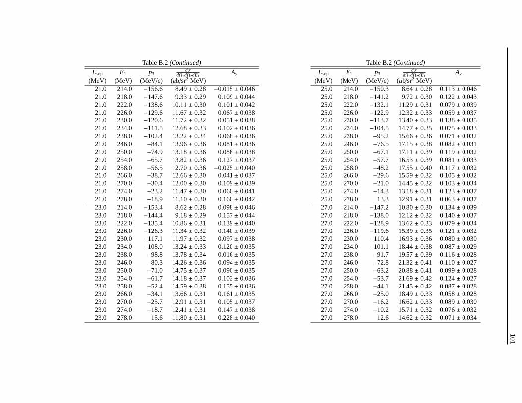
101
Table B.2(Continued)
Esep E1 p3dσ
dΩ1dΩ2dE1Ay
(MeV) (MeV) (MeV/c) (µb/sr2 MeV)21.0 214.0 −156.6 8.49± 0.28 −0.015± 0.04621.0 218.0 −147.6 9.33± 0.29 0.109± 0.04421.0 222.0 −138.6 10.11± 0.30 0.101± 0.04221.0 226.0 −129.6 11.67± 0.32 0.067± 0.03821.0 230.0 −120.6 11.72± 0.32 0.051± 0.03821.0 234.0 −111.5 12.68± 0.33 0.102± 0.03621.0 238.0 −102.4 13.22± 0.34 0.068± 0.03621.0 246.0 −84.1 13.96± 0.36 0.081± 0.03621.0 250.0 −74.9 13.18± 0.36 0.086± 0.03821.0 254.0 −65.7 13.82± 0.36 0.127± 0.03721.0 258.0 −56.5 12.70± 0.36 −0.025± 0.04021.0 266.0 −38.7 12.66± 0.30 0.041± 0.03721.0 270.0 −30.4 12.00± 0.30 0.109± 0.03921.0 274.0 −23.2 11.47± 0.30 0.060± 0.04121.0 278.0 −18.9 11.10± 0.30 0.160± 0.04223.0 214.0 −153.4 8.62± 0.28 0.098± 0.04623.0 218.0 −144.4 9.18± 0.29 0.157± 0.04423.0 222.0 −135.4 10.86± 0.31 0.139± 0.04023.0 226.0 −126.3 11.34± 0.32 0.140± 0.03923.0 230.0 −117.1 11.97± 0.32 0.097± 0.03823.0 234.0 −108.0 13.24± 0.33 0.120± 0.03523.0 238.0 −98.8 13.78± 0.34 0.016± 0.03523.0 246.0 −80.3 14.26± 0.36 0.094± 0.03523.0 250.0 −71.0 14.75± 0.37 0.090± 0.03523.0 254.0 −61.7 14.18± 0.37 0.102± 0.03623.0 258.0 −52.4 14.59± 0.38 0.155± 0.03623.0 266.0 −34.1 13.66± 0.31 0.161± 0.03523.0 270.0 −25.7 12.91± 0.31 0.105± 0.03723.0 274.0 −18.7 12.41± 0.31 0.147± 0.03823.0 278.0 15.6 11.80± 0.31 0.228± 0.040
Table B.2(Continued)
Esep E1 p3dσ
dΩ1dΩ2dE1Ay
(MeV) (MeV) (MeV/c) (µb/sr2 MeV)25.0 214.0 −150.3 8.64± 0.28 0.113± 0.04625.0 218.0 −141.2 9.72± 0.30 0.122± 0.04325.0 222.0 −132.1 11.29± 0.31 0.079± 0.03925.0 226.0 −122.9 12.32± 0.33 0.059± 0.03725.0 230.0 −113.7 13.40± 0.33 0.138± 0.03525.0 234.0 −104.5 14.77± 0.35 0.075± 0.03325.0 238.0 −95.2 15.66± 0.36 0.071± 0.03225.0 246.0 −76.5 17.15± 0.38 0.082± 0.03125.0 250.0 −67.1 17.11± 0.39 0.119± 0.03225.0 254.0 −57.7 16.53± 0.39 0.081± 0.03325.0 258.0 −48.2 17.55± 0.40 0.117± 0.03225.0 266.0 −29.6 15.59± 0.32 0.105± 0.03225.0 270.0 −21.0 14.45± 0.32 0.103± 0.03425.0 274.0 −14.3 13.18± 0.31 0.123± 0.03725.0 278.0 13.3 12.91± 0.31 0.063± 0.03727.0 214.0 −147.2 10.80± 0.30 0.134± 0.03927.0 218.0 −138.0 12.12± 0.32 0.140± 0.03727.0 222.0 −128.9 13.62± 0.33 0.079± 0.03427.0 226.0 −119.6 15.39± 0.35 0.121± 0.03227.0 230.0 −110.4 16.93± 0.36 0.080± 0.03027.0 234.0 −101.1 18.44± 0.38 0.087± 0.02927.0 238.0 −91.7 19.57± 0.39 0.116± 0.02827.0 246.0 −72.8 21.32± 0.41 0.110± 0.02727.0 250.0 −63.2 20.88± 0.41 0.099± 0.02827.0 254.0 −53.7 21.69± 0.42 0.124± 0.02727.0 258.0 −44.1 21.45± 0.42 0.087± 0.02827.0 266.0 −25.0 18.49± 0.33 0.058± 0.02827.0 270.0 −16.2 16.62± 0.33 0.089± 0.03027.0 274.0 −10.2 15.71± 0.32 0.076± 0.03227.0 278.0 12.6 14.62± 0.32 0.071± 0.034
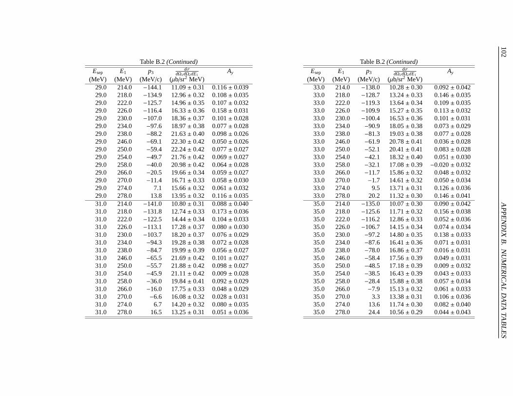
102A
PP
EN
DIX
B.
NU
ME
RIC
AL
DATA
TAB
LES
Table B.2(Continued)
Esep E1 p3dσ
dΩ1dΩ2dE1Ay
(MeV) (MeV) (MeV/c) (µb/sr2 MeV)29.0 214.0 −144.1 11.09± 0.31 0.116± 0.03929.0 218.0 −134.9 12.96± 0.32 0.108± 0.03529.0 222.0 −125.7 14.96± 0.35 0.107± 0.03229.0 226.0 −116.4 16.33± 0.36 0.158± 0.03129.0 230.0 −107.0 18.36± 0.37 0.101± 0.02829.0 234.0 −97.6 18.97± 0.38 0.077± 0.02829.0 238.0 −88.2 21.63± 0.40 0.098± 0.02629.0 246.0 −69.1 22.30± 0.42 0.050± 0.02629.0 250.0 −59.4 22.24± 0.42 0.077± 0.02729.0 254.0 −49.7 21.76± 0.42 0.069± 0.02729.0 258.0 −40.0 20.98± 0.42 0.064± 0.02829.0 266.0 −20.5 19.66± 0.34 0.059± 0.02729.0 270.0 −11.4 16.71± 0.33 0.058± 0.03029.0 274.0 7.1 15.66± 0.32 0.061± 0.03229.0 278.0 13.8 13.95± 0.32 0.116± 0.03531.0 214.0 −141.0 10.80± 0.31 0.088± 0.04031.0 218.0 −131.8 12.74± 0.33 0.173± 0.03631.0 222.0 −122.5 14.44± 0.34 0.104± 0.03331.0 226.0 −113.1 17.28± 0.37 0.080± 0.03031.0 230.0 −103.7 18.20± 0.37 0.076± 0.02931.0 234.0 −94.3 19.28± 0.38 0.072± 0.02831.0 238.0 −84.7 19.99± 0.39 0.056± 0.02731.0 246.0 −65.5 21.69± 0.42 0.101± 0.02731.0 250.0 −55.7 21.88± 0.42 0.098± 0.02731.0 254.0 −45.9 21.11± 0.42 0.009± 0.02831.0 258.0 −36.0 19.84± 0.41 0.092± 0.02931.0 266.0 −16.0 17.75± 0.33 0.048± 0.02931.0 270.0 −6.6 16.08± 0.32 0.028± 0.03131.0 274.0 6.7 14.20± 0.32 0.080± 0.03531.0 278.0 16.5 13.25± 0.31 0.051± 0.036
Table B.2(Continued)
Esep E1 p3dσ
dΩ1dΩ2dE1Ay
(MeV) (MeV) (MeV/c) (µb/sr2 MeV)33.0 214.0 −138.0 10.28± 0.30 0.092± 0.04233.0 218.0 −128.7 13.24± 0.33 0.146± 0.03533.0 222.0 −119.3 13.64± 0.34 0.109± 0.03533.0 226.0 −109.9 15.27± 0.35 0.113± 0.03233.0 230.0 −100.4 16.53± 0.36 0.101± 0.03133.0 234.0 −90.9 18.05± 0.38 0.073± 0.02933.0 238.0 −81.3 19.03± 0.38 0.077± 0.02833.0 246.0 −61.9 20.78± 0.41 0.036± 0.02833.0 250.0 −52.1 20.41± 0.41 0.083± 0.02833.0 254.0 −42.1 18.32± 0.40 0.051± 0.03033.0 258.0 −32.1 17.08± 0.39 −0.020± 0.03233.0 266.0 −11.7 15.86± 0.32 0.048± 0.03233.0 270.0 −1.7 14.61± 0.32 0.050± 0.03433.0 274.0 9.5 13.71± 0.31 0.126± 0.03633.0 278.0 20.2 11.32± 0.30 0.146± 0.04135.0 214.0 −135.0 10.07± 0.30 0.090± 0.04235.0 218.0 −125.6 11.71± 0.32 0.156± 0.03835.0 222.0 −116.2 12.86± 0.33 0.052± 0.03635.0 226.0 −106.7 14.15± 0.34 0.074± 0.03435.0 230.0 −97.2 14.80± 0.35 0.138± 0.03335.0 234.0 −87.6 16.41± 0.36 0.071± 0.03135.0 238.0 −78.0 16.86± 0.37 0.016± 0.03135.0 246.0 −58.4 17.56± 0.39 0.049± 0.03135.0 250.0 −48.5 17.18± 0.39 0.009± 0.03235.0 254.0 −38.5 16.43± 0.39 0.043± 0.03335.0 258.0 −28.4 15.88± 0.38 0.057± 0.03435.0 266.0 −7.9 15.13± 0.32 0.061± 0.03335.0 270.0 3.3 13.38± 0.31 0.106± 0.03635.0 274.0 13.6 11.74± 0.30 0.082± 0.04035.0 278.0 24.4 10.56± 0.29 0.044± 0.043

103
Table B.3: Data table for the40Ca(~p,2p) reaction at the set3 in Table 2.1.∆Esep= 2 MeV.
Esep E1 p3dσ
dΩ1dΩ2dE1Ay
(MeV) (MeV) (MeV/c) (µb/sr2 MeV)29.0 202.0 −147.6 9.30± 0.31 0.106± 0.04529.0 206.0 −139.3 11.25± 0.33 0.198± 0.04029.0 210.0 −130.9 12.39± 0.34 0.147± 0.03829.0 214.0 −122.5 13.30± 0.36 −0.009± 0.03729.0 218.0 −114.2 15.23± 0.38 0.079± 0.03429.0 222.0 −105.8 17.02± 0.39 0.070± 0.03229.0 226.0 −97.5 18.52± 0.41 0.088± 0.03029.0 230.0 −89.2 19.17± 0.41 0.122± 0.02929.0 234.0 −80.9 20.77± 0.43 0.086± 0.02829.0 238.0 −72.8 20.41± 0.43 0.081± 0.02829.0 246.0 −57.0 20.00± 0.31 0.061± 0.02429.0 250.0 −49.5 19.27± 0.31 0.025± 0.02529.0 254.0 −42.7 18.89± 0.31 0.046± 0.02629.0 258.0 −37.0 18.70± 0.31 0.036± 0.02631.0 202.0 −144.4 9.14± 0.31 0.041± 0.04631.0 206.0 −136.0 10.90± 0.33 0.149± 0.04131.0 210.0 −127.5 12.89± 0.35 0.197± 0.03731.0 214.0 −119.1 13.83± 0.36 0.062± 0.03631.0 218.0 −110.6 14.34± 0.37 0.019± 0.03631.0 222.0 −102.2 16.30± 0.39 0.092± 0.03331.0 226.0 −93.7 18.05± 0.41 −0.008± 0.03131.0 230.0 −85.3 18.75± 0.41 0.079± 0.02931.0 234.0 −77.0 19.61± 0.42 0.021± 0.02931.0 238.0 −68.7 20.23± 0.43 0.094± 0.02831.0 246.0 −52.6 18.70± 0.30 0.039± 0.02631.0 250.0 −45.1 18.48± 0.30 0.030± 0.02631.0 254.0 −38.3 18.38± 0.31 0.030± 0.02631.0 258.0 −32.6 17.12± 0.30 0.032± 0.028
Table B.3(Continued)
Esep E1 p3dσ
dΩ1dΩ2dE1Ay
(MeV) (MeV) (MeV/c) (µb/sr2 MeV)33.0 202.0 −141.2 9.69± 0.31 0.083± 0.04433.0 206.0 −132.7 11.04± 0.32 0.104± 0.04033.0 210.0 −124.2 11.85± 0.34 0.101± 0.04033.0 214.0 −115.6 13.56± 0.36 0.085± 0.03733.0 218.0 −107.1 14.92± 0.37 0.040± 0.03533.0 222.0 −98.6 15.63± 0.39 0.168± 0.03433.0 226.0 −90.0 17.68± 0.40 0.150± 0.03133.0 230.0 −81.5 17.64± 0.40 0.037± 0.03133.0 234.0 −73.0 18.24± 0.41 0.025± 0.03033.0 238.0 −64.6 18.61± 0.42 −0.023± 0.03033.0 246.0 −48.2 17.35± 0.30 0.040± 0.02733.0 250.0 −40.6 16.99± 0.30 0.073± 0.02833.0 254.0 −33.7 16.38± 0.30 0.110± 0.02933.0 258.0 −28.3 16.27± 0.30 0.089± 0.02935.0 202.0 −138.0 9.46± 0.31 0.063± 0.04535.0 206.0 −129.4 10.40± 0.32 0.031± 0.04335.0 210.0 −120.8 11.72± 0.34 0.088± 0.04035.0 214.0 −112.2 12.18± 0.35 0.064± 0.04035.0 218.0 −103.6 13.90± 0.37 0.087± 0.03635.0 222.0 −94.9 15.13± 0.38 0.021± 0.03535.0 226.0 −86.3 15.69± 0.39 0.060± 0.03435.0 230.0 −77.7 16.11± 0.39 0.039± 0.03335.0 234.0 −69.1 16.66± 0.40 0.028± 0.03235.0 238.0 −60.5 17.34± 0.41 0.052± 0.03235.0 246.0 −43.9 16.14± 0.29 0.054± 0.02935.0 250.0 −36.1 14.74± 0.29 0.063± 0.03135.0 254.0 −29.2 15.08± 0.29 0.035± 0.03135.0 258.0 −24.1 14.50± 0.29 0.079± 0.032

104A
PP
EN
DIX
B.
NU
ME
RIC
AL
DATA
TAB
LES
Table B.3(Continued)
Esep E1 p3dσ
dΩ1dΩ2dE1Ay
(MeV) (MeV) (MeV/c) (µb/sr2 MeV)37.0 202.0 −134.8 8.56± 0.30 0.061± 0.04937.0 206.0 −126.2 9.73± 0.32 0.082± 0.04537.0 210.0 −117.5 10.47± 0.32 0.067± 0.04337.0 214.0 −108.8 11.46± 0.35 0.041± 0.04237.0 218.0 −100.1 12.46± 0.35 0.065± 0.03937.0 222.0 −91.4 13.40± 0.37 0.041± 0.03837.0 226.0 −82.6 13.74± 0.37 0.020± 0.03737.0 230.0 −73.9 14.39± 0.38 −0.008± 0.03537.0 234.0 −65.1 15.10± 0.39 0.085± 0.03537.0 238.0 −56.4 15.75± 0.39 0.026± 0.03437.0 246.0 −39.5 14.05± 0.28 0.058± 0.03237.0 250.0 −31.5 14.19± 0.28 0.054± 0.03237.0 254.0 −24.7 14.03± 0.29 0.052± 0.03237.0 258.0 −20.0 12.50± 0.28 0.084± 0.03639.0 202.0 −131.7 7.80± 0.30 0.120± 0.05339.0 206.0 −123.0 8.04± 0.30 0.089± 0.05239.0 210.0 −114.2 9.72± 0.32 0.091± 0.04539.0 214.0 −105.4 10.06± 0.33 −0.040± 0.04639.0 218.0 −96.6 10.86± 0.34 0.018± 0.04439.0 222.0 −87.8 11.54± 0.35 0.067± 0.04239.0 226.0 −78.9 11.58± 0.35 0.120± 0.04239.0 230.0 −70.1 12.05± 0.36 0.030± 0.04039.0 234.0 −61.2 12.76± 0.37 0.100± 0.03939.0 238.0 −52.3 13.51± 0.38 0.056± 0.03839.0 246.0 −35.0 12.27± 0.27 0.006± 0.03539.0 250.0 −27.0 12.16± 0.27 −0.007± 0.03639.0 254.0 −20.1 11.66± 0.27 0.109± 0.03739.0 258.0 −16.3 11.46± 0.28 0.059± 0.038
Table B.3(Continued)
Esep E1 p3dσ
dΩ1dΩ2dE1Ay
(MeV) (MeV) (MeV/c) (µb/sr2 MeV)41.0 202.0 −128.6 7.06± 0.29 0.070± 0.05741.0 206.0 −119.8 7.20± 0.29 0.042± 0.05641.0 210.0 −110.9 8.64± 0.31 0.088± 0.04941.0 214.0 −102.1 9.23± 0.33 0.079± 0.04941.0 218.0 −93.2 10.01± 0.33 0.059± 0.04641.0 222.0 −84.3 10.59± 0.34 0.017± 0.04541.0 226.0 −75.3 10.53± 0.35 0.051± 0.04641.0 230.0 −66.3 11.57± 0.35 0.080± 0.04141.0 234.0 −57.3 11.69± 0.36 0.032± 0.04141.0 238.0 −48.3 11.90± 0.37 0.020± 0.04141.0 246.0 −30.6 11.60± 0.27 0.035± 0.03741.0 250.0 −22.3 11.01± 0.27 0.008± 0.03941.0 254.0 −15.6 10.81± 0.27 0.037± 0.04041.0 258.0 13.3 9.96± 0.27 0.083± 0.04343.0 202.0 −125.5 6.81± 0.29 0.036± 0.05843.0 206.0 −116.6 7.22± 0.29 0.139± 0.05643.0 210.0 −107.7 7.48± 0.30 0.052± 0.05543.0 214.0 −98.8 7.97± 0.31 0.055± 0.05443.0 218.0 −89.8 8.74± 0.32 0.026± 0.05143.0 222.0 −80.8 8.75± 0.33 0.035± 0.05143.0 226.0 −71.7 9.90± 0.34 0.067± 0.04743.0 230.0 −62.6 10.70± 0.35 0.037± 0.04443.0 234.0 −53.5 10.85± 0.36 −0.002± 0.04443.0 238.0 −44.3 10.70± 0.36 0.064± 0.04543.0 246.0 −26.2 10.99± 0.27 0.063± 0.03943.0 250.0 −17.7 10.19± 0.27 0.067± 0.04143.0 254.0 −11.2 10.23± 0.27 0.109± 0.04243.0 258.0 11.5 9.94± 0.27 0.068± 0.043

105
Table B.3(Continued)
Esep E1 p3dσ
dΩ1dΩ2dE1Ay
(MeV) (MeV) (MeV/c) (µb/sr2 MeV)45.0 202.0 −122.4 5.95± 0.28 0.003± 0.06545.0 206.0 −113.5 6.28± 0.29 0.133± 0.06345.0 210.0 −104.5 7.25± 0.30 0.110± 0.05745.0 214.0 −95.5 8.09± 0.31 0.055± 0.05345.0 218.0 −86.4 7.84± 0.32 0.073± 0.05545.0 222.0 −77.3 8.33± 0.33 0.148± 0.05445.0 226.0 −68.2 8.59± 0.33 0.077± 0.05345.0 230.0 −58.9 9.66± 0.34 0.019± 0.04745.0 234.0 −49.7 10.21± 0.35 0.012± 0.04645.0 238.0 −40.3 9.93± 0.35 0.097± 0.04845.0 246.0 −21.7 10.63± 0.27 0.015± 0.04045.0 250.0 −13.0 10.10± 0.26 0.069± 0.04245.0 254.0 −7.3 10.17± 0.27 0.084± 0.04245.0 258.0 11.6 10.01± 0.27 0.114± 0.04347.0 202.0 −119.4 6.00± 0.28 0.087± 0.06447.0 206.0 −110.4 6.34± 0.29 0.087± 0.06247.0 210.0 −101.4 6.49± 0.29 0.062± 0.06147.0 214.0 −92.3 6.88± 0.30 0.040± 0.06147.0 218.0 −83.1 7.16± 0.31 0.120± 0.05947.0 222.0 −73.9 7.98± 0.32 0.046± 0.05547.0 226.0 −64.7 9.45± 0.34 0.118± 0.04947.0 230.0 −55.4 10.02± 0.35 0.094± 0.04647.0 234.0 −46.0 10.54± 0.35 0.176± 0.04547.0 238.0 −36.5 9.78± 0.35 0.019± 0.04847.0 246.0 −17.4 10.47± 0.26 0.072± 0.04047.0 250.0 −8.2 10.91± 0.27 0.085± 0.03947.0 254.0 5.1 10.35± 0.27 0.024± 0.04147.0 258.0 13.6 9.62± 0.27 0.073± 0.044
Table B.3(Continued)
Esep E1 p3dσ
dΩ1dΩ2dE1Ay
(MeV) (MeV) (MeV/c) (µb/sr2 MeV)49.0 202.0 −116.4 5.15± 0.27 0.056± 0.07349.0 206.0 −107.3 6.30± 0.28 0.080± 0.06249.0 210.0 −98.2 6.33± 0.29 0.000± 0.06249.0 214.0 −89.1 7.57± 0.31 0.183± 0.05649.0 218.0 −79.9 7.30± 0.31 0.048± 0.05949.0 222.0 −70.6 8.37± 0.32 −0.020± 0.05349.0 226.0 −61.3 8.11± 0.32 0.072± 0.05549.0 230.0 −51.9 9.58± 0.34 0.046± 0.04749.0 234.0 −42.4 9.66± 0.34 0.072± 0.04849.0 238.0 −32.8 9.59± 0.35 0.082± 0.04849.0 246.0 −13.3 10.21± 0.26 0.074± 0.04149.0 250.0 −3.5 10.08± 0.27 0.014± 0.04249.0 254.0 6.8 10.02± 0.27 0.075± 0.04249.0 258.0 17.0 10.31± 0.27 0.063± 0.04151.0 202.0 −113.4 5.07± 0.27 −0.008± 0.07451.0 206.0 −104.3 5.38± 0.28 0.108± 0.07151.0 210.0 −95.2 6.19± 0.28 0.009± 0.06351.0 214.0 −86.0 6.51± 0.30 0.050± 0.06451.0 218.0 −76.7 7.03± 0.31 0.084± 0.06051.0 222.0 −67.4 7.20± 0.31 0.091± 0.06051.0 226.0 −58.0 7.87± 0.32 0.063± 0.05651.0 230.0 −48.5 8.82± 0.34 −0.010± 0.05151.0 234.0 −38.9 9.39± 0.34 0.031± 0.04951.0 238.0 −29.3 9.33± 0.35 −0.021± 0.05051.0 246.0 −9.7 9.82± 0.26 0.032± 0.04251.0 250.0 1.9 9.44± 0.26 0.044± 0.04451.0 254.0 10.8 9.57± 0.26 0.100± 0.04451.0 258.0 21.0 9.42± 0.26 0.069± 0.045

106A
PP
EN
DIX
B.
NU
ME
RIC
AL
DATA
TAB
LES
Table B.3(Continued)
Esep E1 p3dσ
dΩ1dΩ2dE1Ay
(MeV) (MeV) (MeV/c) (µb/sr2 MeV)53.0 202.0 −110.6 5.03± 0.27 0.094± 0.07453.0 206.0 −101.4 5.13± 0.27 0.135± 0.07353.0 210.0 −92.2 5.56± 0.28 −0.058± 0.07053.0 214.0 −83.0 6.11± 0.30 0.095± 0.06753.0 218.0 −73.7 6.36± 0.30 0.070± 0.06553.0 222.0 −64.3 6.56± 0.30 0.083± 0.06453.0 226.0 −54.8 7.81± 0.32 0.085± 0.05653.0 230.0 −45.3 8.30± 0.33 0.110± 0.05353.0 234.0 −35.7 8.43± 0.33 0.032± 0.05353.0 238.0 −26.1 9.08± 0.34 0.047± 0.05153.0 246.0 −7.6 8.80± 0.26 0.018± 0.04753.0 250.0 6.5 9.44± 0.26 0.065± 0.04453.0 254.0 15.4 9.15± 0.26 0.059± 0.04553.0 258.0 25.5 8.80± 0.26 0.034± 0.047
Table B.4: Data table for the40Ca(~p,2p) reaction at the set4 in Table 2.1.∆Esep= 2 MeV.
Esep E1 p3dσ
dΩ1dΩ2dE1Ay
(MeV) (MeV) (MeV/c) (µb/sr2 MeV)41.0 186.0 −140.9 5.57± 0.36 0.088± 0.09641.0 190.0 −133.0 6.41± 0.37 0.051± 0.08741.0 194.0 −125.1 7.55± 0.39 0.104± 0.07841.0 202.0 −109.3 7.55± 0.32 −0.004± 0.06341.0 206.0 −101.5 8.64± 0.33 −0.043± 0.05741.0 210.0 −93.7 8.83± 0.34 −0.079± 0.05741.0 214.0 −86.0 9.23± 0.32 0.031± 0.04941.0 218.0 −78.3 9.74± 0.33 0.127± 0.04841.0 222.0 −70.9 9.15± 0.32 0.090± 0.05141.0 226.0 −63.6 10.75± 0.34 −0.046± 0.04541.0 230.0 −56.6 9.30± 0.26 −0.017± 0.04541.0 234.0 −50.1 9.78± 0.27 0.066± 0.04341.0 238.0 −44.3 9.93± 0.27 0.040± 0.04343.0 186.0 −137.8 5.20± 0.35 0.156± 0.10143.0 190.0 −129.7 5.57± 0.36 0.051± 0.09843.0 194.0 −121.7 6.25± 0.37 −0.054± 0.09043.0 202.0 −105.8 7.35± 0.32 0.117± 0.06343.0 206.0 −97.9 7.09± 0.32 0.056± 0.06543.0 210.0 −90.0 8.59± 0.34 0.032± 0.05843.0 214.0 −82.1 8.48± 0.31 0.086± 0.05243.0 218.0 −74.4 8.76± 0.32 −0.007± 0.05243.0 222.0 −66.8 9.69± 0.33 0.078± 0.04843.0 226.0 −59.4 9.23± 0.33 0.050± 0.05143.0 230.0 −52.3 9.28± 0.26 0.094± 0.04543.0 234.0 −45.7 8.67± 0.26 0.000± 0.04843.0 238.0 −39.9 8.75± 0.27 0.056± 0.048

107
Table B.4(Continued)
Esep E1 p3dσ
dΩ1dΩ2dE1Ay
(MeV) (MeV) (MeV/c) (µb/sr2 MeV)45.0 186.0 −134.6 4.84± 0.35 0.296± 0.10945.0 190.0 −126.5 4.95± 0.35 0.195± 0.10545.0 194.0 −118.4 6.70± 0.37 0.147± 0.08445.0 202.0 −102.3 6.52± 0.31 0.017± 0.06945.0 206.0 −94.3 7.16± 0.32 0.083± 0.06645.0 210.0 −86.3 7.44± 0.32 −0.024± 0.06445.0 214.0 −78.3 8.03± 0.31 0.038± 0.05545.0 218.0 −70.4 8.51± 0.31 0.038± 0.05345.0 222.0 −62.7 9.02± 0.32 0.003± 0.05145.0 226.0 −55.2 8.94± 0.33 0.056± 0.05245.0 230.0 −48.0 9.34± 0.26 0.019± 0.04445.0 234.0 −41.3 8.82± 0.26 0.052± 0.04745.0 238.0 −35.5 9.35± 0.27 0.020± 0.04547.0 186.0 −131.5 4.89± 0.35 0.116± 0.10847.0 190.0 −123.3 5.04± 0.35 −0.049± 0.10647.0 194.0 −115.1 5.93± 0.37 0.099± 0.09447.0 202.0 −98.8 6.30± 0.31 0.267± 0.07247.0 206.0 −90.7 6.72± 0.31 −0.034± 0.06947.0 210.0 −82.6 7.77± 0.33 0.075± 0.06247.0 214.0 −74.5 8.11± 0.31 0.022± 0.05447.0 218.0 −66.5 7.63± 0.31 −0.092± 0.05847.0 222.0 −58.6 8.95± 0.32 0.059± 0.05147.0 226.0 −50.9 9.31± 0.33 −0.032± 0.05147.0 230.0 −43.6 8.81± 0.26 −0.018± 0.04747.0 234.0 −36.8 9.02± 0.27 −0.009± 0.04747.0 238.0 −31.1 8.72± 0.26 0.084± 0.048
Table B.4(Continued)
Esep E1 p3dσ
dΩ1dΩ2dE1Ay
(MeV) (MeV) (MeV/c) (µb/sr2 MeV)49.0 186.0 −128.3 5.44± 0.36 0.092± 0.09849.0 190.0 −120.1 4.80± 0.35 0.102± 0.11049.0 194.0 −111.9 5.47± 0.36 0.023± 0.10049.0 202.0 −95.4 6.27± 0.31 0.107± 0.07149.0 206.0 −87.1 7.08± 0.32 0.092± 0.06649.0 210.0 −78.9 6.85± 0.32 −0.002± 0.06949.0 214.0 −70.7 6.94± 0.30 0.092± 0.06249.0 218.0 −62.6 8.34± 0.31 0.066± 0.05449.0 222.0 −54.5 8.36± 0.32 0.058± 0.05449.0 226.0 −46.7 8.86± 0.33 0.046± 0.05349.0 230.0 −39.2 8.56± 0.26 0.110± 0.04849.0 234.0 −32.4 8.59± 0.26 0.096± 0.04849.0 238.0 −26.7 8.72± 0.27 0.096± 0.04851.0 186.0 −125.3 4.30± 0.34 −0.056± 0.12051.0 190.0 −116.9 4.98± 0.35 −0.098± 0.10751.0 194.0 −108.6 5.34± 0.36 0.132± 0.10151.0 202.0 −91.9 5.95± 0.30 −0.038± 0.07551.0 206.0 −83.6 6.71± 0.32 0.011± 0.06951.0 210.0 −75.3 6.77± 0.32 0.124± 0.06951.0 214.0 −66.9 7.20± 0.30 0.117± 0.05951.0 218.0 −58.7 8.29± 0.32 0.093± 0.05451.0 222.0 −50.5 8.26± 0.32 0.051± 0.05551.0 226.0 −42.4 9.08± 0.33 0.126± 0.05251.0 230.0 −34.8 8.03± 0.26 0.019± 0.05151.0 234.0 −27.9 8.58± 0.26 −0.031± 0.04951.0 238.0 −22.4 8.39± 0.27 0.102± 0.050

108A
PP
EN
DIX
B.
NU
ME
RIC
AL
DATA
TAB
LES
Table B.4(Continued)
Esep E1 p3dσ
dΩ1dΩ2dE1Ay
(MeV) (MeV) (MeV/c) (µb/sr2 MeV)53.0 186.0 −122.2 4.82± 0.35 0.015± 0.11153.0 190.0 −113.8 4.70± 0.35 −0.001± 0.11353.0 194.0 −105.4 4.63± 0.35 −0.075± 0.11453.0 202.0 −88.5 5.08± 0.30 0.034± 0.08653.0 206.0 −80.1 6.07± 0.31 0.031± 0.07653.0 210.0 −71.6 6.35± 0.32 0.074± 0.07353.0 214.0 −63.2 7.45± 0.30 0.044± 0.05853.0 218.0 −54.8 7.42± 0.30 −0.014± 0.05953.0 222.0 −46.4 8.00± 0.32 −0.024± 0.05653.0 226.0 −38.2 8.26± 0.32 0.020± 0.05653.0 230.0 −30.4 7.91± 0.26 0.038± 0.05153.0 234.0 −23.3 8.51± 0.26 0.063± 0.04953.0 238.0 −18.1 7.95± 0.26 0.016± 0.05355.0 186.0 −119.2 4.08± 0.34 0.183± 0.12555.0 190.0 −110.7 4.66± 0.35 −0.070± 0.11355.0 194.0 −102.2 4.77± 0.35 −0.038± 0.11055.0 202.0 −85.2 5.12± 0.30 0.083± 0.08655.0 206.0 −76.6 4.99± 0.30 −0.002± 0.08855.0 210.0 −68.1 6.60± 0.32 0.044± 0.07155.0 214.0 −59.5 7.01± 0.30 0.070± 0.06155.0 218.0 −50.9 7.47± 0.31 −0.005± 0.05955.0 222.0 −42.4 7.37± 0.31 0.033± 0.06055.0 226.0 −34.0 8.08± 0.32 0.087± 0.05655.0 230.0 −25.9 7.70± 0.26 −0.080± 0.05355.0 234.0 −18.7 7.79± 0.26 0.122± 0.05355.0 238.0 −14.1 7.79± 0.26 0.016± 0.054
Table B.4(Continued)
Esep E1 p3dσ
dΩ1dΩ2dE1Ay
(MeV) (MeV) (MeV/c) (µb/sr2 MeV)57.0 186.0 −116.2 3.74± 0.33 −0.038± 0.13557.0 190.0 −107.6 4.34± 0.34 −0.134± 0.12057.0 194.0 −99.1 4.43± 0.35 0.125± 0.11957.0 202.0 −81.9 5.08± 0.30 0.237± 0.08557.0 206.0 −73.2 5.48± 0.31 0.068± 0.08257.0 210.0 −64.5 6.15± 0.32 0.050± 0.07557.0 214.0 −55.8 5.90± 0.29 0.016± 0.07057.0 218.0 −47.1 7.23± 0.30 −0.103± 0.06157.0 222.0 −38.4 7.03± 0.31 0.029± 0.06357.0 226.0 −29.7 7.64± 0.32 0.076± 0.05957.0 230.0 −21.4 6.60± 0.25 0.041± 0.06057.0 234.0 −14.1 7.06± 0.26 0.032± 0.05857.0 238.0 10.5 7.39± 0.26 0.081± 0.05659.0 186.0 −113.2 3.90± 0.34 0.007± 0.13159.0 190.0 −104.6 4.05± 0.34 −0.011± 0.12759.0 194.0 −96.0 4.21± 0.34 0.083± 0.12359.0 202.0 −78.6 4.17± 0.29 0.138± 0.10259.0 206.0 −69.9 5.10± 0.30 0.071± 0.08659.0 210.0 −61.1 5.38± 0.31 −0.097± 0.08459.0 214.0 −52.2 6.02± 0.29 −0.028± 0.07059.0 218.0 −43.3 6.68± 0.30 0.050± 0.06459.0 222.0 −34.4 6.41± 0.30 −0.094± 0.06859.0 226.0 −25.6 7.04± 0.31 −0.044± 0.06359.0 230.0 −17.0 6.59± 0.25 −0.032± 0.06059.0 234.0 −9.5 6.88± 0.25 −0.032± 0.05959.0 238.0 8.2 6.93± 0.26 0.079± 0.059

109
Table B.4(Continued)
Esep E1 p3dσ
dΩ1dΩ2dE1Ay
(MeV) (MeV) (MeV/c) (µb/sr2 MeV)61.0 186.0 −110.3 3.99± 0.34 0.033± 0.13061.0 190.0 −101.7 4.39± 0.35 0.138± 0.11861.0 194.0 −93.0 4.66± 0.35 0.085± 0.11461.0 202.0 −75.4 5.32± 0.30 0.110± 0.08261.0 206.0 −66.6 5.95± 0.31 0.146± 0.07561.0 210.0 −57.7 5.33± 0.30 0.023± 0.08461.0 214.0 −48.7 6.01± 0.29 0.014± 0.07061.0 218.0 −39.7 6.12± 0.30 0.108± 0.06961.0 222.0 −30.6 6.21± 0.30 0.053± 0.06961.0 226.0 −21.5 6.71± 0.31 0.075± 0.06561.0 230.0 −12.6 6.03± 0.25 −0.072± 0.06561.0 234.0 −4.9 6.27± 0.25 0.049± 0.06361.0 238.0 8.4 5.97± 0.25 0.045± 0.06763.0 186.0 −107.5 3.71± 0.34 −0.241± 0.13963.0 190.0 −98.8 4.09± 0.34 0.033± 0.12663.0 194.0 −90.0 4.44± 0.35 0.107± 0.11863.0 202.0 −72.3 3.99± 0.29 −0.161± 0.10763.0 206.0 −63.4 5.11± 0.30 −0.026± 0.08663.0 210.0 −54.4 5.24± 0.30 −0.009± 0.08563.0 214.0 −45.4 5.73± 0.29 −0.037± 0.07263.0 218.0 −36.2 5.15± 0.29 −0.021± 0.07963.0 222.0 −27.0 5.88± 0.30 0.112± 0.07263.0 226.0 −17.7 5.99± 0.30 0.081± 0.07263.0 230.0 −8.4 5.98± 0.25 −0.002± 0.06663.0 234.0 1.7 5.51± 0.25 0.075± 0.07163.0 238.0 10.9 5.61± 0.25 −0.020± 0.072
Table B.4(Continued)
Esep E1 p3dσ
dΩ1dΩ2dE1Ay
(MeV) (MeV) (MeV/c) (µb/sr2 MeV)65.0 186.0 −104.7 3.78± 0.33 0.085± 0.13365.0 190.0 −95.9 3.92± 0.34 0.124± 0.13065.0 194.0 −87.1 4.31± 0.35 0.039± 0.12165.0 202.0 −69.3 4.42± 0.29 −0.038± 0.09665.0 206.0 −60.3 4.74± 0.30 0.151± 0.09265.0 210.0 −51.3 4.27± 0.29 0.109± 0.10165.0 214.0 −42.2 5.61± 0.29 −0.033± 0.07465.0 218.0 −33.0 5.52± 0.29 0.201± 0.07565.0 222.0 −23.7 5.82± 0.29 0.084± 0.07265.0 226.0 −14.4 5.70± 0.30 0.077± 0.07465.0 230.0 −5.1 4.86± 0.24 −0.097± 0.07965.0 234.0 5.3 4.72± 0.24 −0.055± 0.08165.0 238.0 14.7 4.50± 0.24 0.084± 0.08667.0 186.0 −102.0 3.40± 0.33 0.244± 0.14867.0 190.0 −93.1 3.35± 0.33 0.181± 0.15067.0 194.0 −84.3 3.99± 0.34 −0.097± 0.12967.0 202.0 −66.4 3.89± 0.28 −0.048± 0.10767.0 206.0 −57.4 4.05± 0.29 −0.039± 0.10567.0 210.0 −48.3 4.47± 0.30 0.092± 0.09767.0 214.0 −39.2 5.14± 0.28 −0.029± 0.07967.0 218.0 −30.0 4.68± 0.29 0.004± 0.08767.0 222.0 −20.8 5.69± 0.29 0.125± 0.07367.0 226.0 −11.8 5.04± 0.29 0.124± 0.08267.0 230.0 −5.2 4.58± 0.24 −0.079± 0.08367.0 234.0 10.0 4.80± 0.24 0.045± 0.08067.0 238.0 19.1 4.27± 0.24 −0.022± 0.090

110A
PP
EN
DIX
B.
NU
ME
RIC
AL
DATA
TAB
LES
Table B.4(Continued)
Esep E1 p3dσ
dΩ1dΩ2dE1Ay
(MeV) (MeV) (MeV/c) (µb/sr2 MeV)69.0 186.0 −99.3 3.19± 0.34 0.358± 0.15969.0 190.0 −90.5 3.08± 0.33 0.389± 0.16269.0 194.0 −81.6 3.44± 0.33 0.160± 0.14669.0 202.0 −63.6 3.71± 0.29 −0.037± 0.11369.0 206.0 −54.6 4.02± 0.29 0.021± 0.10669.0 210.0 −45.5 4.28± 0.29 0.039± 0.09969.0 214.0 −36.5 4.72± 0.28 0.132± 0.08469.0 218.0 −27.4 4.73± 0.28 0.057± 0.08669.0 222.0 −18.6 4.80± 0.29 −0.137± 0.08669.0 226.0 −10.9 5.13± 0.29 0.066± 0.08169.0 230.0 8.6 4.27± 0.24 −0.102± 0.08969.0 234.0 14.8 4.12± 0.24 −0.021± 0.09169.0 238.0 23.8 4.09± 0.24 −0.058± 0.09471.0 186.0 −96.8 3.64± 0.33 0.012± 0.13871.0 190.0 −87.9 3.11± 0.33 0.083± 0.15971.0 194.0 −79.0 3.46± 0.33 −0.132± 0.14271.0 202.0 −61.0 3.85± 0.28 0.013± 0.10871.0 206.0 −52.0 3.76± 0.29 0.116± 0.11171.0 210.0 −43.0 3.62± 0.29 −0.039± 0.11671.0 214.0 −34.1 4.41± 0.28 −0.029± 0.09171.0 218.0 −25.4 4.32± 0.28 −0.117± 0.09271.0 222.0 −17.4 4.81± 0.28 −0.017± 0.08471.0 226.0 −11.9 4.01± 0.28 0.034± 0.09971.0 230.0 13.0 4.18± 0.24 0.073± 0.08971.0 234.0 19.8 4.15± 0.24 −0.102± 0.09271.0 238.0 28.6 3.55± 0.23 0.017± 0.104
Table B.4(Continued)
Esep E1 p3dσ
dΩ1dΩ2dE1Ay
(MeV) (MeV) (MeV/c) (µb/sr2 MeV)73.0 186.0 −94.3 2.75± 0.32 −0.129± 0.17473.0 190.0 −85.4 3.07± 0.33 0.306± 0.16073.0 194.0 −76.5 3.47± 0.33 0.089± 0.14573.0 202.0 −58.6 2.90± 0.28 −0.064± 0.14073.0 206.0 −49.7 3.59± 0.28 0.180± 0.11673.0 210.0 −40.8 4.15± 0.29 −0.076± 0.10273.0 214.0 −32.2 3.96± 0.27 0.023± 0.09973.0 218.0 −24.1 4.10± 0.28 0.182± 0.09773.0 222.0 −17.4 3.88± 0.28 −0.031± 0.10373.0 226.0 −14.5 3.86± 0.28 0.122± 0.10273.0 230.0 17.6 3.68± 0.23 −0.052± 0.10173.0 234.0 24.7 3.33± 0.23 0.262± 0.11173.0 238.0 33.5 3.08± 0.23 −0.134± 0.121
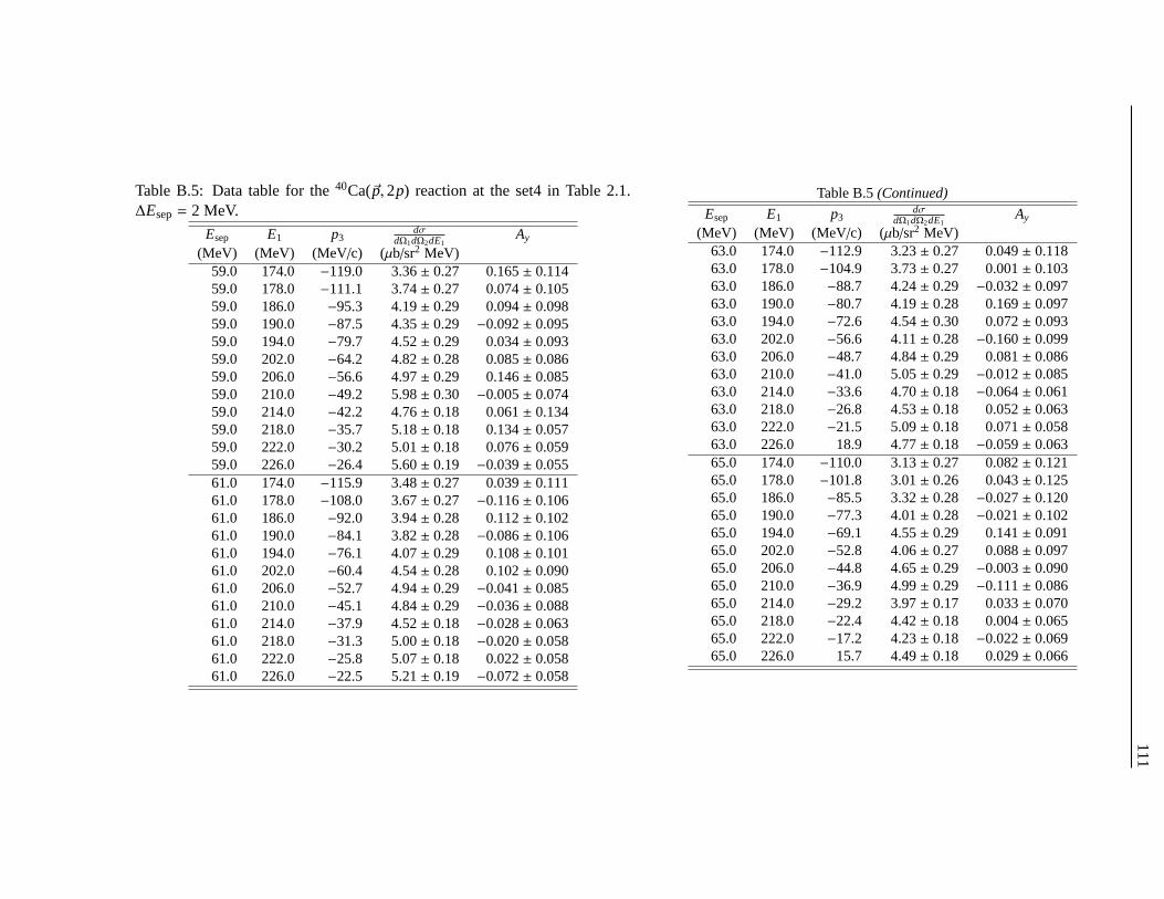
111
Table B.5: Data table for the40Ca(~p,2p) reaction at the set4 in Table 2.1.∆Esep= 2 MeV.
Esep E1 p3dσ
dΩ1dΩ2dE1Ay
(MeV) (MeV) (MeV/c) (µb/sr2 MeV)59.0 174.0 −119.0 3.36± 0.27 0.165± 0.11459.0 178.0 −111.1 3.74± 0.27 0.074± 0.10559.0 186.0 −95.3 4.19± 0.29 0.094± 0.09859.0 190.0 −87.5 4.35± 0.29 −0.092± 0.09559.0 194.0 −79.7 4.52± 0.29 0.034± 0.09359.0 202.0 −64.2 4.82± 0.28 0.085± 0.08659.0 206.0 −56.6 4.97± 0.29 0.146± 0.08559.0 210.0 −49.2 5.98± 0.30 −0.005± 0.07459.0 214.0 −42.2 4.76± 0.18 0.061± 0.13459.0 218.0 −35.7 5.18± 0.18 0.134± 0.05759.0 222.0 −30.2 5.01± 0.18 0.076± 0.05959.0 226.0 −26.4 5.60± 0.19 −0.039± 0.05561.0 174.0 −115.9 3.48± 0.27 0.039± 0.11161.0 178.0 −108.0 3.67± 0.27 −0.116± 0.10661.0 186.0 −92.0 3.94± 0.28 0.112± 0.10261.0 190.0 −84.1 3.82± 0.28 −0.086± 0.10661.0 194.0 −76.1 4.07± 0.29 0.108± 0.10161.0 202.0 −60.4 4.54± 0.28 0.102± 0.09061.0 206.0 −52.7 4.94± 0.29 −0.041± 0.08561.0 210.0 −45.1 4.84± 0.29 −0.036± 0.08861.0 214.0 −37.9 4.52± 0.18 −0.028± 0.06361.0 218.0 −31.3 5.00± 0.18 −0.020± 0.05861.0 222.0 −25.8 5.07± 0.18 0.022± 0.05861.0 226.0 −22.5 5.21± 0.19 −0.072± 0.058
Table B.5(Continued)
Esep E1 p3dσ
dΩ1dΩ2dE1Ay
(MeV) (MeV) (MeV/c) (µb/sr2 MeV)63.0 174.0 −112.9 3.23± 0.27 0.049± 0.11863.0 178.0 −104.9 3.73± 0.27 0.001± 0.10363.0 186.0 −88.7 4.24± 0.29 −0.032± 0.09763.0 190.0 −80.7 4.19± 0.28 0.169± 0.09763.0 194.0 −72.6 4.54± 0.30 0.072± 0.09363.0 202.0 −56.6 4.11± 0.28 −0.160± 0.09963.0 206.0 −48.7 4.84± 0.29 0.081± 0.08663.0 210.0 −41.0 5.05± 0.29 −0.012± 0.08563.0 214.0 −33.6 4.70± 0.18 −0.064± 0.06163.0 218.0 −26.8 4.53± 0.18 0.052± 0.06363.0 222.0 −21.5 5.09± 0.18 0.071± 0.05863.0 226.0 18.9 4.77± 0.18 −0.059± 0.06365.0 174.0 −110.0 3.13± 0.27 0.082± 0.12165.0 178.0 −101.8 3.01± 0.26 0.043± 0.12565.0 186.0 −85.5 3.32± 0.28 −0.027± 0.12065.0 190.0 −77.3 4.01± 0.28 −0.021± 0.10265.0 194.0 −69.1 4.55± 0.29 0.141± 0.09165.0 202.0 −52.8 4.06± 0.27 0.088± 0.09765.0 206.0 −44.8 4.65± 0.29 −0.003± 0.09065.0 210.0 −36.9 4.99± 0.29 −0.111± 0.08665.0 214.0 −29.2 3.97± 0.17 0.033± 0.07065.0 218.0 −22.4 4.42± 0.18 0.004± 0.06565.0 222.0 −17.2 4.23± 0.18 −0.022± 0.06965.0 226.0 15.7 4.49± 0.18 0.029± 0.066
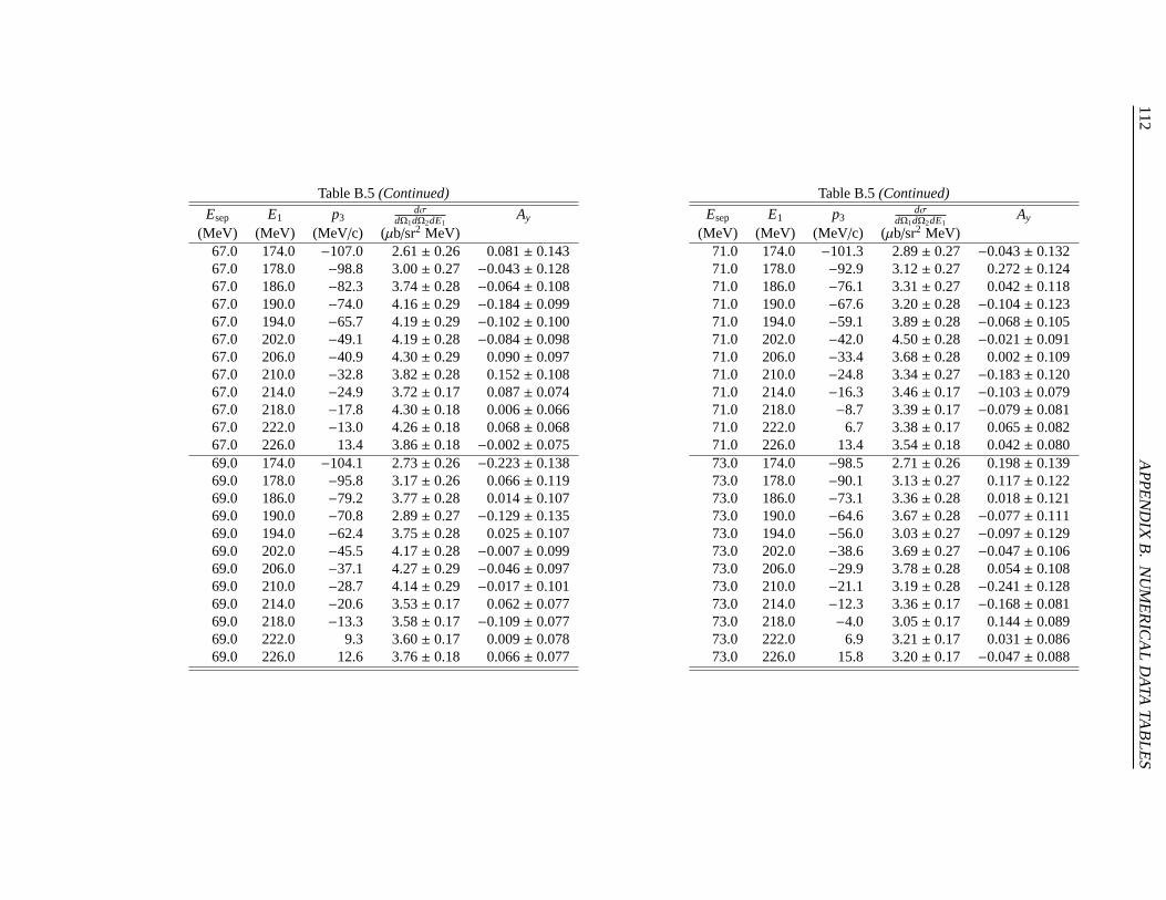
112A
PP
EN
DIX
B.
NU
ME
RIC
AL
DATA
TAB
LES
Table B.5(Continued)
Esep E1 p3dσ
dΩ1dΩ2dE1Ay
(MeV) (MeV) (MeV/c) (µb/sr2 MeV)67.0 174.0 −107.0 2.61± 0.26 0.081± 0.14367.0 178.0 −98.8 3.00± 0.27 −0.043± 0.12867.0 186.0 −82.3 3.74± 0.28 −0.064± 0.10867.0 190.0 −74.0 4.16± 0.29 −0.184± 0.09967.0 194.0 −65.7 4.19± 0.29 −0.102± 0.10067.0 202.0 −49.1 4.19± 0.28 −0.084± 0.09867.0 206.0 −40.9 4.30± 0.29 0.090± 0.09767.0 210.0 −32.8 3.82± 0.28 0.152± 0.10867.0 214.0 −24.9 3.72± 0.17 0.087± 0.07467.0 218.0 −17.8 4.30± 0.18 0.006± 0.06667.0 222.0 −13.0 4.26± 0.18 0.068± 0.06867.0 226.0 13.4 3.86± 0.18 −0.002± 0.07569.0 174.0 −104.1 2.73± 0.26 −0.223± 0.13869.0 178.0 −95.8 3.17± 0.26 0.066± 0.11969.0 186.0 −79.2 3.77± 0.28 0.014± 0.10769.0 190.0 −70.8 2.89± 0.27 −0.129± 0.13569.0 194.0 −62.4 3.75± 0.28 0.025± 0.10769.0 202.0 −45.5 4.17± 0.28 −0.007± 0.09969.0 206.0 −37.1 4.27± 0.29 −0.046± 0.09769.0 210.0 −28.7 4.14± 0.29 −0.017± 0.10169.0 214.0 −20.6 3.53± 0.17 0.062± 0.07769.0 218.0 −13.3 3.58± 0.17 −0.109± 0.07769.0 222.0 9.3 3.60± 0.17 0.009± 0.07869.0 226.0 12.6 3.76± 0.18 0.066± 0.077
Table B.5(Continued)
Esep E1 p3dσ
dΩ1dΩ2dE1Ay
(MeV) (MeV) (MeV/c) (µb/sr2 MeV)71.0 174.0 −101.3 2.89± 0.27 −0.043± 0.13271.0 178.0 −92.9 3.12± 0.27 0.272± 0.12471.0 186.0 −76.1 3.31± 0.27 0.042± 0.11871.0 190.0 −67.6 3.20± 0.28 −0.104± 0.12371.0 194.0 −59.1 3.89± 0.28 −0.068± 0.10571.0 202.0 −42.0 4.50± 0.28 −0.021± 0.09171.0 206.0 −33.4 3.68± 0.28 0.002± 0.10971.0 210.0 −24.8 3.34± 0.27 −0.183± 0.12071.0 214.0 −16.3 3.46± 0.17 −0.103± 0.07971.0 218.0 −8.7 3.39± 0.17 −0.079± 0.08171.0 222.0 6.7 3.38± 0.17 0.065± 0.08271.0 226.0 13.4 3.54± 0.18 0.042± 0.08073.0 174.0 −98.5 2.71± 0.26 0.198± 0.13973.0 178.0 −90.1 3.13± 0.27 0.117± 0.12273.0 186.0 −73.1 3.36± 0.28 0.018± 0.12173.0 190.0 −64.6 3.67± 0.28 −0.077± 0.11173.0 194.0 −56.0 3.03± 0.27 −0.097± 0.12973.0 202.0 −38.6 3.69± 0.27 −0.047± 0.10673.0 206.0 −29.9 3.78± 0.28 0.054± 0.10873.0 210.0 −21.1 3.19± 0.28 −0.241± 0.12873.0 214.0 −12.3 3.36± 0.17 −0.168± 0.08173.0 218.0 −4.0 3.05± 0.17 0.144± 0.08973.0 222.0 6.9 3.21± 0.17 0.031± 0.08673.0 226.0 15.8 3.20± 0.17 −0.047± 0.088

113
Table B.5(Continued)
Esep E1 p3dσ
dΩ1dΩ2dE1Ay
(MeV) (MeV) (MeV/c) (µb/sr2 MeV)75.0 174.0 −95.9 2.25± 0.25 −0.200± 0.16275.0 178.0 −87.4 2.68± 0.26 −0.042± 0.13875.0 186.0 −70.3 3.39± 0.28 0.037± 0.11775.0 190.0 −61.6 3.26± 0.27 0.136± 0.12075.0 194.0 −53.0 3.33± 0.27 0.182± 0.11875.0 202.0 −35.4 2.72± 0.27 −0.077± 0.14175.0 206.0 −26.6 3.36± 0.28 −0.192± 0.12175.0 210.0 −17.6 3.36± 0.28 0.075± 0.11975.0 214.0 −8.6 3.10± 0.17 0.027± 0.08775.0 218.0 0.7 3.11± 0.17 −0.045± 0.08875.0 222.0 9.8 2.74± 0.17 −0.044± 0.09975.0 226.0 19.1 3.13± 0.17 0.018± 0.08977.0 174.0 −93.2 2.51± 0.26 −0.085± 0.14777.0 178.0 −84.7 2.56± 0.26 0.001± 0.14377.0 186.0 −67.5 2.96± 0.27 0.026± 0.13077.0 190.0 −58.8 2.90± 0.27 −0.202± 0.13677.0 194.0 −50.1 3.20± 0.28 −0.001± 0.12477.0 202.0 −32.5 3.15± 0.27 0.035± 0.12577.0 206.0 −23.7 2.78± 0.27 0.006± 0.14277.0 210.0 −14.8 2.97± 0.27 0.086± 0.13577.0 214.0 −6.4 2.89± 0.17 −0.129± 0.09377.0 218.0 5.4 2.76± 0.17 −0.021± 0.09777.0 222.0 13.8 2.84± 0.17 0.023± 0.09577.0 226.0 23.1 2.77± 0.17 −0.060± 0.101
Table B.5(Continued)
Esep E1 p3dσ
dΩ1dΩ2dE1Ay
(MeV) (MeV) (MeV/c) (µb/sr2 MeV)79.0 174.0 −90.7 2.31± 0.26 0.103± 0.15979.0 178.0 −82.1 3.13± 0.26 −0.043± 0.12079.0 186.0 −64.9 2.87± 0.27 0.001± 0.13579.0 190.0 −56.2 2.85± 0.27 0.051± 0.13679.0 194.0 −47.4 3.01± 0.27 0.315± 0.13179.0 202.0 −29.9 2.78± 0.27 0.058± 0.14279.0 206.0 −21.3 2.59± 0.27 0.070± 0.14979.0 210.0 −13.0 2.79± 0.27 0.127± 0.14379.0 214.0 −7.1 2.69± 0.16 −0.082± 0.09979.0 218.0 10.1 2.64± 0.16 −0.057± 0.10179.0 222.0 18.3 2.57± 0.17 −0.056± 0.10579.0 226.0 27.4 2.63± 0.17 0.022± 0.10381.0 174.0 −88.3 2.78± 0.26 0.109± 0.13581.0 178.0 −79.7 2.51± 0.26 −0.012± 0.14881.0 186.0 −62.4 2.55± 0.27 0.055± 0.15181.0 190.0 −53.7 2.76± 0.27 0.137± 0.14281.0 194.0 −45.0 2.51± 0.27 −0.069± 0.15381.0 202.0 −27.8 2.51± 0.27 0.122± 0.15581.0 206.0 −19.6 2.52± 0.27 0.327± 0.15481.0 210.0 −12.6 2.37± 0.27 0.219± 0.15881.0 214.0 10.2 2.45± 0.16 −0.037± 0.10681.0 218.0 14.9 2.47± 0.17 −0.014± 0.10881.0 222.0 22.9 2.31± 0.16 −0.138± 0.11681.0 226.0 31.9 2.76± 0.17 −0.002± 0.099
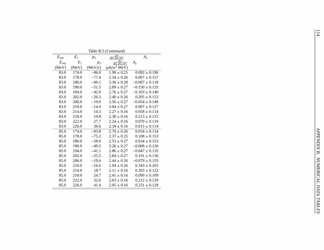
114A
PP
EN
DIX
B.
NU
ME
RIC
AL
DATA
TAB
LES
Table B.5(Continued)
Esep E1 p3dσ
dΩ1dΩ2dE1Ay
Esep E1 p3dσ
dΩ1dΩ2dE1Ay
(MeV) (MeV) (MeV/c) (µb/sr2 MeV)83.0 174.0 −86.0 1.90± 0.25 0.092± 0.19083.0 178.0 −77.4 2.34± 0.26 0.007± 0.15783.0 186.0 −60.1 3.36± 0.28 −0.007± 0.11883.0 190.0 −51.5 2.89± 0.27 −0.150± 0.13583.0 194.0 −42.9 2.76± 0.27 −0.103± 0.14083.0 202.0 −26.3 2.40± 0.26 0.205± 0.15383.0 206.0 −19.0 2.56± 0.27 −0.054± 0.14983.0 210.0 −14.0 3.04± 0.27 0.007± 0.12783.0 214.0 14.3 2.27± 0.16 0.058± 0.11483.0 218.0 19.8 2.30± 0.16 0.213± 0.11583.0 222.0 27.7 2.24± 0.16 0.070± 0.11983.0 226.0 36.6 2.34± 0.16 0.015± 0.11485.0 174.0 −83.8 2.79± 0.26 0.034± 0.13485.0 178.0 −75.2 2.37± 0.25 0.108± 0.15385.0 186.0 −58.0 2.53± 0.27 0.034± 0.15385.0 190.0 −49.5 3.26± 0.27 −0.008± 0.12085.0 194.0 −41.1 2.86± 0.27 −0.047± 0.13585.0 202.0 −25.5 2.84± 0.27 0.101± 0.13685.0 206.0 −19.4 2.44± 0.26 −0.079± 0.15585.0 210.0 −16.6 1.94± 0.26 0.343± 0.20385.0 214.0 18.7 2.11± 0.16 0.203± 0.12285.0 218.0 24.7 2.41± 0.16 0.099± 0.10985.0 222.0 32.6 2.03± 0.16 0.212± 0.12985.0 226.0 41.4 2.05± 0.16 0.231± 0.128

Bibliography
[1] T. Otsuka, R. Fujimoto, Y. Utsuno, B. A. Brown, M. Honma, and T. Mizusaki, Phys. Rev. Lett.87,
082502 (Aug 2001)
[2] T. Otsuka, T. Suzuki, R. Fujimoto, H. Grawe, and Y. Akaishi, Phys. Rev. Lett.95, 232502 (Nov
2005)
[3] R. A. Niyazov, L. B. Weinstein, G. Adams, P. Ambrozewicz, E. Anciant, M. Anghinolfi, B. Asava-
pibhop, G. Asryan, G. Audit, T. Auger, H. Avakian, H. Bagdasaryan, J. P. Ball, S. Barrow,
M. Battaglieri, K. Beard, M. Bektasoglu, M. Bellis, N. Benmouna, B. L. Berman, W. Bertozzi,
N. Bianchi, A. S. Biselli, S. Boiarinov, B. E. Bonner, S. Bouchigny, andR. Bradford, Phys. Rev.
Lett. 92, 052303 (Feb 2004)
[4] R. Shneor, P. Monaghan, R. Subedi, B. D. Anderson, K. Aniol, J. Annand, J. Arrington, H. Be-
naoum, F. Benmokhtar, P. Bertin, W. Bertozzi, W. Boeglin, J. P. Chen, S. Choi, E. Chudakov,
E. Cisbani, B. Craver, C. W. de Jager, R. J. Feuerbach, S. Frullani,F. Garibaldi, O. Gayou, S. Gi-
lad, R. Gilman, O. Glamazdin, J. Gomez, and J.-O. Hansen, Phys. Rev. Lett.99, 072501 (Aug
2007)
[5] D. L. Groep, M. F. van Batenburg, T. S. Bauer, H. P. Blok, D. J.Boersma, E. Cisbani, R. De Leo,
S. Frullani, F. Garibaldi, W. Glockle, J. Golak, P. Heimberg, W. H. A. Hesselink, M. Iodice, D. G.
Ireland, E. Jans, H. Kamada, L. Lapikas, G. J. Lolos, C. J. G. Onderwater, R. Perrino, A. Scott,
R. Starink, M. F. M. Steenbakkers, G. M. Urciuoli, H. de Vries, L. B. Weinstein, and H. Witała,
Phys. Rev. C63, 014005 (Dec 2000)
[6] D. Middleton, J. Annand, C. Barbieri, P. Barneo, H. Blok, R. Bohm,M. Distler, J. Friedrich,
C. Giusti, D. Glazier, P. Grabmayr, T. Hehl, J. Heim, W. Hesselink, E. Jans, M. Kohl, L. Lapikas,
I. MacGregor, I. Martin, J. McGeorge, H. Merkel, F. Moschini, G. Rosner, M. Seimetz, H. de Vries,
T. Walcher, D. Watts, and B. Zihlmann, The European Physical JournalA - Hadrons and Nuclei
29, 261 (2006), ISSN 1434-6001
[7] D. G. Middleton, J. R. M. Annand, M. A. Antelo, C. Ayerbe, P. Barneo, D. Baumann, J. Bermuth,
J. Bernauer, H. P. Blok, R. Bohm, D. Bosnar, M. Ding, M. O. Distler, J. Friedrich, J. G. Llongo,
D. I. Glazier, J. Golak, W. Glockle, P. Grabmayr, T. Hehl, J. Heim, W. H. A. Hesselink, E. Jans,
H. Kamada, G. J. Manas, M. Kohl, L. Lapikas, I. J. D. MacGregor, I. Martin, J. C. McGeorge,
115

116 BIBLIOGRAPHY
H. Merkel, P. Merle, K. Monstad, F. Moschini, U. Muller, A. Nogga, R. Perez-Benito, T. Pospis-
chil, M. Potokar, G. Rosner, M. Seimetz, R. Skibinski, H. de Vries, T. Walcher, D. P. Watts,
M. Weinriefer, M. Weiss, H. Witała, and B. Zihlmann, Phys. Rev. Lett.103, 152501 (Oct 2009)
[8] J. Aclander, J. Alster, D. Barton, G. Bunce, A. Carroll, N. Christensen, H. Courant, S. Durrant,
S. Gushue, S. Heppelmann, E. Kosonovsky, I. Mardor, Y. Mardor,M. Marshak, Y. Makdisi, E. Mi-
nor, I. Navon, H. Nicholson, E. Piasetzky, T. Roser, J. Russell, M. Sargsian, C. Sutton, M. Tanaka,
C. White, and J.-Y. Wu, Physics Letters B453, 211 (1999)
[9] A. Tang, J. W. Watson, J. Aclander, J. Alster, G. Asryan, Y. Averichev, D. Barton, V. Baturin,
N. Bukhtoyarova, A. Carroll, S. Gushue, S. Heppelmann, A. Leksanov, Y. Makdisi, A. Malki,
E. Minina, I. Navon, H. Nicholson, A. Ogawa, Y. Panebratsev, E. Piasetzky, A. Schetkovsky,
S. Shimanskiy, and D. Zhalov, Phys. Rev. Lett.90, 042301 (Jan 2003)
[10] P. Doll, G. J. Wagner, K. T. Knvpfle, and G. Mairle, Nuclear Physics A 263, 210 (1976)
[11] A. E. L. Dieperink and P. K. A. Huberts, Annual Review of Nuclear and Particle Science40, 239
(1990)
[12] L. Lapikas, Nuclear Physics A553, 297c (1993)
[13] O. Benhar, A. Fabrocini, and S. Fantoni, Phys. Rev. C41, R24 (Jan 1990)
[14] R. Jastrow, Phys. Rev.98, 1479 (Jun 1955)
[15] J. G. Zabolitzky and W. Ey, Physics Letters B76, 527 (1978)
[16] O. Bohigas and S. Stringari, Physics Letters B95, 9 (1980)
[17] M. Dal Ri, S. Stringari, and O. Bohigas, Nuclear Physics A376, 81 (1982)
[18] F. Dellagiacoma, G. Orlandini, and M. Traini, Nuclear Physics A393, 95 (1983)
[19] M. Jaminon, C. Mahaux, and H. Ngt, Nuclear Physics A473, 509 (1987)
[20] A. Fabrocini and G. Co’, Phys. Rev. C63, 044319 (Mar 2001)
[21] C. Bisconti, F. A. d. Saavedra, and G. Co’, Phys. Rev. C75, 054302 (May 2007)
[22] J. Mougey, M. Bernheim, A. A. Bussiere, A. Gillebert, P. X. Ho, M. Priou, D. Royer, I. Sick, and
G. J. Wagner, Nuclear Physics A262, 461 (1976)
[23] K. Nakamura, S. Hiramatsu, T. Kamae, H. Muramatsu, N. Izutsu, andY. Watase, Phys. Rev. Lett.
33, 853 (Sep 1974)
[24] K. Nakamura, S. Hiramatsu, T. Kamae, H. Muramatsu, N. Izutsu, andY. Watase, Nuclear Physics
A 271, 221 (1976)

BIBLIOGRAPHY 117
[25] U. Amaldi Jr., G. C. Venuti, G. Cortellessa, E. D. Sanctis, S. Frullani,R. Lombard, and P. Salvadori,
Physics Letters22, 593 (1966)
[26] A. N. James, P. T. Andrews, P. Kirkby, and B. G. Lowe, NuclearPhysics A138, 145 (1969)
[27] S. Kullander, F. Lemeilleur, P. Renberg, G. Landaud, J. Yonnet,B. Fagerstrvm, A. Johansson, and
G. Tibell, Nuclear Physics A173, 357 (1971)
[28] O. Chamberlain and E. Segre, Phys. Rev.87, 81 (Jul 1952)
[29] J. B. Cladis, W. N. Hess, and B. J. Moyer, Phys. Rev.87, 425 (Aug 1952)
[30] G. JACOB and T. A. J. MARIS, Rev. Mod. Phys.38, 121 (Jan 1966)
[31] G. JACOB and T. A. J. MARIS, Rev. Mod. Phys.45, 6 (Jan 1973)
[32] P. Kitching, W. McDonald, T. Maris, and C. Vasconcellos, inADVANCES IN NUCLEAR PHYSICS,
Vol. 15, edited by J. W. Negele and E. Vogt (PLENUM PRESS, 1985) Chap. 2, pp. 43–83
[33] G. Jacob, T. A. J. Maris, C. Schneider, and M. R. Teodoro, Physics Letters B45, 181 (1973), ISSN
0370-2693
[34] P. Kitching, C. A. Miller, D. A. Hutcheon, A. N. James, W. J. McDonald, J. M. Cameron, W. C.
Olsen, and G. Roy, Phys. Rev. Lett.37, 1600 (Dec 1976)
[35] P. Kitching, C. A. Miller, W. C. Olsen, D. A. Hutcheon, W. J. McDonald, and A. W. Stetz, Nuclear
Physics A340, 423 (1980), ISSN 0375-9474
[36] L. Antonuk, P. Kitching, C. A. Miller, D. A. Hutcheon, W. J. McDonald, G. C. Neilson, W. C.
Olsen, and A. W. Stetz, Nuclear Physics A370, 389 (1981), ISSN 0375-9474
[37] W. J. McDonald, R. N. MacDonald, W. C. Olsen, R. Dymarz, F. Khanna, L. Antonuk, J. M.
Cameron, P. Kitching, G. C. Neilson, D. M. Sheppard, D. A. Hutcheon, C. A. Miller, and J. Kallne,
Nuclear Physics A456, 577 (1986), ISSN 0375-9474
[38] G. JACOB and T. A. J. MARIS, Rev. Mod. Phys.45, 6 (Jan 1973)
[39] P. G. Roos, N. S. Chant, D. W. Devins, D. L. Friesel, W. P. Jones, A. C. Attard, R. S. Henderson,
I. D. Svalbe, B. M. Spicer, V. C. Officer, and G. G. Shute, Phys. Rev. Lett.40, 1439 (May 1978)
[40] C. Samanta, N. S. Chant, P. G. Roos, A. Nadasen, J. Wesick, andA. A. Cowley, Phys. Rev. C34,
1610 (Nov 1986)
[41] A. A. Cowley, J. V. Pilcher, J. J. Lawrie, and D. M. Whittal, Phys. Rev. C40, 1950 (Nov 1989)
[42] A. A. Cowley, J. J. Lawrie, G. C. Hillhouse, D. M. Whittal, S. V. Fortsch, J. V. Pilcher, F. D. Smit,
and P. G. Roos, Phys. Rev. C44, 329 (Jul 1991)
[43] A. A. Cowley, G. J. Arendse, J. A. Stander, and W. A. Richter, Physics Letters B359, 300 (1995)

118 BIBLIOGRAPHY
[44] R. Neveling, A. A. Cowley, G. F. Steyn, S. V. Fortsch, G. C. Hillhouse, J. Mano, and S. M.
Wyngaardt, Phys. Rev. C66, 034602 (Sep 2002)
[45] C. A. Miller, K. H. Hicks, R. Abegg, M. Ahmad, N. S. Chant, D. Frekers, P. W. Green, L. G.
Greeniaus, D. A. Hutcheon, P. Kitching, D. J. Mack, W. J. McDonald, W. C. Olsen, R. Schubank,
P. G. Roos, and Y. Ye, Phys. Rev. C57, 1756 (Apr 1998)
[46] K. Hatanaka, M. Kawabata, N. Matsuoka, Y. Mizuno, S. Morinobu, M. Nakamura, T. Noro, A. Ok-
ihana, K. Sagara, K. Takahisa, H. Takeda, K. Tamura, M. Tanaka, S. Toyama, H. Yamazaki, and
Y. Yuasa, Phys. Rev. Lett.78, 1014 (Feb 1997)
[47] T. Noro, T. Baba, K. Hatanaka, M. Ito, M. K. N. Matsuoka, H. Sakaguchi, K. Takahisa, H. Takeda,
A. Tamii, K. Tamura, H. Yoshida, and M. Yosoi, RCNP annual report(1996)
[48] T. Noro, T. Yonemura, S. Asaji, N. S. Chant, K. Fujita, Y. Hagihara, K. Hatanaka, G. C. Hillhouse,
T. Ishida, M. Itoh, S. Kishi, M. Nakamura, Y. Nagasue, H. Sakaguchi,Y. Sakemi, Y. Shimizu,
H. Takeda, Y. Tamesige, S. Terashima, M. Uchida, T. Wakasa, Y. Yasuda, H. P. Yoshida, and
M. Yosoi, Phys. Rev. C72, 041602 (2005)
[49] V. A. Andreev, M. N. Andronenko, G. M. Amalsky, S. L. Belostotski, O. A. Domchenkov, O. Y.
Fedorov, K. Hatanaka, A. A. Izotov, A. A. Jgoun, J. Kamiya, A. Y. Kisselev, M. A. Kopytin, O. V.
Miklukho, Y. G. Naryshkin, T. Noro, E. Obayashi, A. N. Prokofiev, D. A. Prokofiev, H. Sakaguchi,
V. V. Sulimov, A. V. Shvedchikov, H. Takeda, S. I. Trush, V. V. Vikhrov, T. Wakasa, Y. Yasuda,
and H. P. Yoshida, Phys. Rev. C69, 024604 (Feb 2004)
[50] S. Frullani and J. Mougey, inADVANCES IN NUCLEAR PHYSICS, Vol. 14, edited by J. W. Negele
and E. Vogt (PLENUM PRESS, 1984) pp. 1–283
[51] J. Kelly, in ADVANCES IN NUCLEAR PHYSICS, Vol. 23, edited by J. W. Negele and E. Vogt
(PLENUM PRESS, 1996) Chap. 2, pp. 75–294
[52] G. J. Kramer, H. P. Blok, and L. Lapikas, Nuclear Physics A679, 267 (2001)
[53] S. S. Volkov, A. A. Vorob’ev, O. A. Domchenkov, Y. V. Dotsenko, N. P. Kuropatkin, A. A. Lobo-
denko, O. V. Miklukho, V. N. Nikulin, V. E. Stradubsky, A. Y. Tsaregorodtsev, Z. A. Chakhalyan,
and Y. A. Shcheglov, Soviet Journal of Nuclear Physics52, 848 (1990)
[54] A. A. Vorob’ev, Y. V. Dotsenko, A. A. Lobodenko, O. V. Miklukho, I. I. Tkach, A. Y. Tsaregorodt-
sev, and Y. A. Shcheglov, Physics of Atomic Nuclei58, 1817 (1995)
[55] Y. Yasuda, Master’s thesis, Kyoto University (2001)
[56] K. Hatanaka, K. Takahisa, H. Tamura, M. Sato, and I. Miura, Nuclear Instruments and Methods
in Physics Research Section A: Accelerators, Spectrometers, Detectorsand Associated Equipment
384, 575 (1997)
BIBLIOGRAPHY 119
[57] I. Miura, T. Yamazaki, A. Shimizu, K. Hosono, T. Itahashi, T. Saito,A. Ando, K. Tamura,
K. Hatanaka, M. Kibayashi, M. Uraki, H. Ogata, M. Kondo, and H. Ikegami, in Proceedings
of the 13th International Conference on Cyclotrons and their Applications, Vancouver, edited by
G. Dutte and M. K. Craddock (World Scientific, Singapore, 1993) p. 3
[58] T. Wakasa, K. Hatanaka, Y. Fujita, G. P. A. Berg, H. Fujimura, H. Fujita, M. Itoh, J. Kamiya,
T. Kawabata, K. Nagayama, T. Noro, H. Sakaguchi, Y. Shimbara, H. Takeda, K. Tamura, H. Ueno,
M. Uchida, M. Uraki, and M. Yosoi, Nuclear Instruments and Methods in Physics Research Section
A: Accelerators, Spectrometers, Detectors and Associated Equipment482, 79 (2002)
[59] M. Fujiwara, H. Akimune, I. Daito, H. Fujimura, Y. Fujita, K. Hatanaka,H. Ikegami, I. Katayama,
K. Nagayama, N. Matsuoka, S. Morinobu, T. Noro, M. Yoshimura, H. Sakaguchi, Y. Sakemi,
A. Tamii, and M. Yosoi, Nuclear Instruments and Methods in Physics Research Section A: Accel-
erators, Spectrometers, Detectors and Associated Equipment422, 484 (1999)
[60] M. Fujiwara, A. Nakanishi, Y. Fujita, N. Matsuoka, T. Noro, S. Morinobu, and H. Ikegami, RCNP
annual report(1989)
[61] N. Matsuoka, T. Noro, K. Sagara, S. Morinobu, A. Okihara, and K. Hatanaka, RCNP annual
report(1990)
[62] N. Matsuoka, T. Noro, K. Sagara, S. Morinobu, A. Okihara, and K. Hatanaka, RCNP annual
report(1991)
[63] T. Noro, M. Fujiwara, O. Kamigaito, S. Hirata, Y. Fujita, A. Yamagoshi,T. Takahashi, H. Akimune,
Y. Sakemi, M. Yosoi, H. Sakaguchi, and J. Tanaka, RCNP annual report(1991)
[64] A. Tamii, H. Sakaguchi, H. Takeda, M. Yosoi, H. Akimune, M. Fujiwara, H. Ogata, M. Tanaka,
and H. Togawa, IEEE Transactions on Nuclear Science43, 2488 (1996)
[65] A. Tamii, M. Itoh, T. Kawabata, H. Sakaguchi, H. Takeda, T. Taki,H. Torii, M. Yosoi, H. Akimune,
T. Baba, M. Fujiwara, M. Kawabata, T. Noro, , and H. Yoshida, inProceedings of the 2nd Inter-
national Data Acquisition Workshop on Networked Data Acquisition System, Osaka, Japan, 1996,
edited by M. Nomachi and S. Ajimura (World Scientific, Singapore, 1997) p.238
[66] T. Kawabata, H. Sakaguchi, A. Tamii, H. Takeda, T. Taki, and H. Yoshida, RCNP annual re-
port(1996)
[67] H. Takeda, H. Sakaguchi, A. Tamii, H. Akimune, M. Kawabata, and M. Tanaka, inProceedings of
the 1995 IEEE Conference on Real-Time Computer Applications in Nuclear Particle and Plasma
Physics (1995) p. 210
[68] HBOOK, CERN Program Library entry Y250
[69] PAW, CERN Program Library entry Q121

120 BIBLIOGRAPHY
[70] M. Ieiri, H. Sakaguchi, M. Nakamura, H. Sakamoto, H. Ogawa, M. Yosol, T. Ichihara, N. Isshiki,
Y. Takeuchi, H. Togawa, T. Tsutsumi, S. Hirata, T. Nakano, S. Kobayashi, T. Noro, and H. Ikegami,
Nuclear Instruments and Methods in Physics Research Section A: Accelerators, Spectrometers,
Detectors and Associated Equipment257, 253 (1987)
[71] N. Fujita, Calibrations of the absolute value of the cross sections for the elastic scattering via
300MeV proton, Master’s thesis, University of Miyazaki (2009)
[72] L. Ray, Phys. Rev. C20, 1857 (Nov 1979)
[73] R. A. Arndt, W. J. Briscoe, I. I. Strakovsky, and R. L. Workman, Phys. Rev. C76, 025209 (Aug
2007)
[74] Center for Nuclear Studies, Data Analysis Center, SAID Program,http://gwdac.phys.gwu.
edu/
[75] N. S. Chant and P. G. Roos, Phys. Rev. C27, 1060 (Mar 1983)
[76] R. A. Arndt, J. S. Hyslop, and L. D. Roper, Phys. Rev. D35, 128 (Jan 1987)
[77] E. D. Cooper, S. Hama, B. C. Clark, and R. L. Mercer, Phys. Rev. C 47, 297 (Jan 1993)
[78] L. R. B. Elton and A. Swift, Nuclear Physics A94, 52 (1967)
[79] G. Kramer, H. Blok, J. V. D. Brand, H. Bulten, R. Ent, E. Jans, J.Lanen, L. Lapikas, H. Nann,
E. Quint, G. V. D. Steenhoven, P. D. W. Huberts, and G. Wagner, Physics Letters B227, 199
(1989)
[80] I. Angeli, Atomic Data and Nuclear Data Tables87, 185 (2004)
[81] H. Sakaguchi, M. Nakamura, K. Hatanaka, A. Goto, T. Noro, F. Ohtani, H. Sakamoto, H. Ogawa,
and S. Kobayashi, Phys. Rev. C26, 944 (Sep 1982)
[82] J. W. A. den Herder, H. P. Blok, E. Jans, P. H. M. Keizer, L. Lapikas, E. N. M. Quint, G. van der
Steenhoven, and P. K. A. de Witt Huberts, Nuclear Physics A490, 507 (1988)
[83] R. B. Firestone and C. M. Baglin,Table of Isotopes, 8th ed. (John Wiley & Sons.Inc., 1999)
[84] Y. Kudo and K. Miyazaki, Phys. Rev. C34, 1192 (Oct 1986)
[85] J. Mano and Y. Kudo, Progress of Theoretical Physics100, 91 (1998)
[86] J. C. Hiebert, E. Newman, and R. H. Bassel, Phys. Rev.154, 898 (Feb 1967)
[87] O. V. Miklukho, N. P. Aleshin, S. L. Belostotski, Y. V. Elkin, O. G. Grebenyuk, O. Y. Fedorov,
A. A. Izotov, A. A. Jgoun, A. Y. Kisselev, M. P. Levchenko, Y. G. Naryskin, V. V. Nelyubin, A. N.
Prokofiev, D. A. Prokofiev, Y. A. Scheglov, A. V. Shvedchikov, V.V. Vikhrov, and A. A. Zhdanov,
Nuclear Physics A683, 145 (2001)
BIBLIOGRAPHY 121
[88] A. A. Cowley, G. J. Arendse, R. F. Visser, G. F. Steyn, S. V. Fortsch, J. J. Lawrie, J. V. Pilcher,
T. Noro, T. Baba, K. Hatanaka, M. Kawabata, N. Matsuoka, Y. Mizuno, M. Nomachi, K. Takahisa,
K. Tamura, Y. Yuasa, H. Sakaguchi, T. Itoh, H. Takeda, and Y. Watanabe, Phys. Rev. C57, 3185
(Jun 1998)
[89] R. Sartor and C. Mahaux, Phys. Rev. C21, 2613 (Jun 1980)
[90] S. Terashima, H. Sakaguchi, H. Takeda, T. Ishikawa, M. Itoh, T. Kawabata, T. Murakami,
M. Uchida, Y. Yasuda, M. Yosoi, J. Zenihiro, H. P. Yoshida, T. Noro,T. Ishida, S. Asaji, and
T. Yonemura, Phys. Rev. C77, 024317 (Feb 2008)
[91] S. Hama, B. C. Clark, E. D. Cooper, H. S. Sherif, and R. L. Mercer, Phys. Rev. C41, 2737 (Jun
1990)
[92] F. Perey and B. Buck, Nuclear Physics32, 353 (1962), ISSN 0029-5582
[93] K. G. Fissum, M. Liang, B. D. Anderson, K. A. Aniol, L. Auerbach, F. T. Baker, J. Berthot,
W. Bertozzi, P.-Y. Bertin, L. Bimbot, W. U. Boeglin, E. J. Brash, V. Breton, H. Breuer, E. Burtin,
J. R. Calarco, L. S. Cardman, G. D. Cates, C. Cavata, C. C. Chang, J.-P. Chen, E. Cisbani, D. S.
Dale, C. W. de Jager, R. De Leo, A. Deur, and B. Diederich, Phys. Rev. C 70, 034606 (Sep 2004)
[94] A. Gade, D. Bazin, B. A. Brown, C. M. Campbell, J. A. Church, D.C. Dinca, J. Enders, T. Glas-
macher, P. G. Hansen, Z. Hu, K. W. Kemper, W. F. Mueller, H. Olliver, B. C. Perry, L. A. Riley,
B. T. Roeder, B. M. Sherrill, J. R. Terry, J. A. Tostevin, and K. L. Yurkewicz, Phys. Rev. Lett.93,
042501 (Jul 2004)
[95] A. Gade, P. Adrich, D. Bazin, M. D. Bowen, B. A. Brown, C. M. Campbell, J. M. Cook, T. Glas-
macher, P. G. Hansen, K. Hosier, S. McDaniel, D. McGlinchery, A. Obertelli, K. Siwek, L. A.
Riley, J. A. Tostevin, and D. Weisshaar, Phys. Rev. C77, 044306 (Apr 2008)
[96] R. J. Charity, L. G. Sobotka, and W. H. Dickhoff, Phys. Rev. Lett.97, 162503 (Oct 2006)
[97] Y. Nagasue, Master’s thesis, Kyushu University (2006)
[98] A. Werbrouck, inKinematics and Multiparticle Systems, edited by M. Nikolic (GORDON AND
BREACH, 1968)

122 BIBLIOGRAPHY
List of Tables
2.1 Measured kinematical sets (central values). The angle of the GR was fixed at 25.5.
θLAS indicates the angle of the LAS which was set according to the measured separation-
energy region. . . . . . . . . . . . . . . . . . . . . . . . . . . . . . . . . . . . . . . 14
2.2 Targets used in the measurements. . . . . . . . . . . . . . . . . . . . . . . . . . .. . 16
2.3 Design specification of Grand Raiden spectrometer (GR). . . . . . . . . .. . . . . . . 17
2.4 Design specification of Large Acceptance Spectrometer (LAS). . . . .. . . . . . . . . 18
2.5 Specifications of the MDWCs for Grand Raiden. . . . . . . . . . . . . . . . .. . . . 21
2.6 Specifications of the MDWCs for LAS. . . . . . . . . . . . . . . . . . . . . . . .. . 21
2.7 Specifications of the MWPCs for GR and LAS. . . . . . . . . . . . . . . . . . .. . . 22
4.1 Bound-state parameters of the Woods-Saxon potential for40Ca nucleus. . . . . . . . . 44
5.1 Spectroscopic factors for the discrete peaks in the40Ca measurement. Krameret al.
reanalyzed the previous (d,3He) data of Dollet al. in Ref. [10] in their study [52]. The
present result is shown with the uncertainty obtained in the fitting or MDA. . . .. . . 58
5.2 Centroid energies and widths (FWHM) of the strength distributions for thehole states of
the 1p and 1s1/2 orbitals in40Ca. For the present result, the uncertainties were obtained
as the region corresponding to a change of 1 inχ2 from the minimum value in the fitting
of the asymmetric Lorenzian and the background. . . . . . . . . . . . . . . . . .. . 61
5.3 Spectroscopic factors relative to the IPSM limits for the orbitals in40Ca. They are
obtained after the background subtraction in the present study. The second uncertainty,
in parenthesised, was estimated by the propagation of the strength uncertainties at each
2-MeV bin and the uncertainty of the contribution of the background. The first one
includes also the model uncertainty, which is mentioned in the text. . . . . . . . . . .62
123

124 LIST OF TABLES
5.4 Spectroscopic factors relative to the IPSM limits for the orbitals in40Ca without back-
ground subtraction. The uncertainty was estimated by the propagation of thestrength
uncertainties at each 2-MeV bin. . . . . . . . . . . . . . . . . . . . . . . . . . . . .. 62
6.1 Global optical potentials used for the distortion in the DWIA calculation. . . .. . . . 77
6.2 Normalized spectroscopic factors relative to the IPSM limits for the orbitals in40Ca.
The description of the uncertainty is same as Table 5.3 except that these uncertainties
include also the uncertainty of the normalization. . . . . . . . . . . . . . . . . . . . .82
6.3 Spectroscopic factors relative to the IPSM limits for the orbitals in40Ca obtained from
previous experiments. For the present result, the description of the uncertainty is same
as Table 6.2. . . . . . . . . . . . . . . . . . . . . . . . . . . . . . . . . . . . . . . . 86
6.4 Spectroscopic factors relative to the IPSM limits for the orbitals in40Ca obtained from
theoretical studies. For the present result, the description of the uncertainty is same as
Table 6.2. . . . . . . . . . . . . . . . . . . . . . . . . . . . . . . . . . . . . . . . . . 86
B.1 Data table for the40Ca(~p,2p) reaction for the peaks at 8.3 and 10.9 MeV in the separa-
tion energy at the set1 in Table 2.1. . . . . . . . . . . . . . . . . . . . . . . . . . . . 99
B.2 Data table for the40Ca(~p,2p) reaction at the set2 in Table 2.1.∆Esep= 2 MeV. . . . . 100
B.3 Data table for the40Ca(~p,2p) reaction at the set3 in Table 2.1.∆Esep= 2 MeV. . . . . 103
B.4 Data table for the40Ca(~p,2p) reaction at the set4 in Table 2.1.∆Esep= 2 MeV. . . . . 106
B.5 Data table for the40Ca(~p,2p) reaction at the set4 in Table 2.1.∆Esep= 2 MeV. . . . . 111

List of Figures
1.1 Summed spectroscopic strength observed for proton knockout fromvarious orbitals in
the closed-shell nuclei16O, 40Ca,48Ca,90Zr, and208Pb as a function of the mean excita-
tion energy of the orbital relative to the Fermi energy (ǫF) The dashed curve represents
the quasi-particle strength calculated for nuclear matter, the solid curve is derived from
the nuclear matter curve by including surface effects calculated for208Pb [13]. This
figure is taken from Ref. [12]. . . . . . . . . . . . . . . . . . . . . . . . . . . . .. . 3
1.2 Analyzing powers for the 1p3/2 and p1/2-hole states for16O(p,2p) reaction measured
by changing a kinetic energy of an ejected proton. They behave differently as predicted
by Jacob and Maris and show the validity of Maris effect. This figure is taken from
Ref. [35] . . . . . . . . . . . . . . . . . . . . . . . . . . . . . . . . . . . . . . . . . 5
1.3 Separation energies, widths, and angular momentum assignments of the hole states ob-
tained from quasi-free scattering, as functions of the atomic number. This figure is taken
from Ref. [38] . . . . . . . . . . . . . . . . . . . . . . . . . . . . . . . . . . . . . . 6
1.4 Separation-energy spectra for40Ca(p,2p) (upper three figures ) and40Ca(p, pn) (lower
three figures ) reactions measured with a 1 GeV proton beam at Petersburg Nuclear
Physics Institute (PNPI) from Ref. [53]. The detection range of protonenergy is (a)
830–870, (b) 855–887, and (c) 880–915 MeV. . . . . . . . . . . . . . . .. . . . . . . 8
2.1 Schematic view of the RCNP ring cyclotron facility. . . . . . . . . . . . . . . . . .. 12
2.2 Notation for the kinematics of theA(p,2p)B reaction in the laboratory system. The inci-
dent energy of the proton isT0 = 392 MeV in the present study. The recoil momentum
of the residual nucleusB is indicated byp3. . . . . . . . . . . . . . . . . . . . . . . . 13
2.3 Layout of BLP. . . . . . . . . . . . . . . . . . . . . . . . . . . . . . . . . . . . . .. 15
2.4 Schematic view of the dual-arm spectrometer system at RCNP. . . . . . . . .. . . . . 16
2.5 Focal plane detectors of the GR. . . . . . . . . . . . . . . . . . . . . . . . . . .. . . 18
2.6 Structure of each plane of MWDC. . . . . . . . . . . . . . . . . . . . . . . . . .. . . 19
125

126 LIST OF FIGURES
2.7 Wire configurations of the X-plane and U-plane of the GR-MWDC. . . . .. . . . . . 19
2.8 Focal plane detectors of the LAS. . . . . . . . . . . . . . . . . . . . . . . . . .. . . . 20
2.9 Wire configurations of the X-plane, U-plane, and V-plane of the LAS-MWDC. . . . . 22
2.10 Schematic view of the layout around the scattering chamber. The protonbeam is injected
into the reaction target at the center of the scattering chamber and is transported to the
Faraday cup placed about 25 m downstream of the target. The MWPCs and the lead
collimators are installed in front of the quadrupole magnets. . . . . . . . . . . . .. . 23
2.11 Geometrical relation of anode planes of the MWPC and the center of the scattering
chamber. . . . . . . . . . . . . . . . . . . . . . . . . . . . . . . . . . . . . . . . . . 24
2.12 Structure of each wire plane of the MWPCs. . . . . . . . . . . . . . . . . . .. . . . 24
2.13 Logic diagram for the GR focal plane detectors. . . . . . . . . . . . . . .. . . . . . . 25
2.14 Logic diagram for the LAS focal plane detectors. . . . . . . . . . . . . .. . . . . . . 26
2.15 Logic diagram for coincidence event of the GR and LAS. . . . . . . . .. . . . . . . . 26
2.16 Schematic view of the data acquisition system. . . . . . . . . . . . . . . . . . . . .. 27
3.1 Energy loss spectrum from the PS1 of the GR, which is the mean of the pulse-height
signals of the left and right PMTs. . . . . . . . . . . . . . . . . . . . . . . . . . . .. 31
3.2 (a):TDC spectrum that indicates the time difference between the mean-time signal from
PS1 of the GR and the RF signal from the AVF cyclotron. The RF signal wasfiltered
at the half rate. (b): TDC spectrum corrected by the trajectory angle andthe position at
the focal plane so that the influence of the momentum acceptance of the spectrometer
on the TDC is eliminated. . . . . . . . . . . . . . . . . . . . . . . . . . . . . . . . . 32
3.3 Two-dimensional scatter plot of the corrected TDC and∆E1 of the GR. The events
enclosed by the solid lines are recognized as the proton events. . . . . . . .. . . . . . 33
3.4 TDC spectrum for the time difference between the GR and LAS trigger signals in a
measurement of the40Ca(p,2p) reaction. . . . . . . . . . . . . . . . . . . . . . . . . 34
3.5 position in a plane of MWDC . . . . . . . . . . . . . . . . . . . . . . . . . . . . . . . 34
3.6 Coordinate systems for the ray-tracing with two MWDCs. . . . . . . . . . . . .. . . 35
3.7 Two dimensional scatter plot of the horizontal and vertical scattering angles of protons
analyzed with the GR (a) and LAS (b). . . . . . . . . . . . . . . . . . . . . . . . . .. 39

LIST OF FIGURES 127
3.8 (a): Two dimensional scatter plot of the energies of coincidence two protons measured
with the GR and LAS in the40Ca(p,2p) reaction atT0 = 392 MeV. (b): Separation-
energy spectrum for the40Ca(p,2p) reaction. Separation energy spectrum . . . . . . . 41
4.1 Recoil-momentum distributions of the cross sections for the 1s1/2-, 1p3/2-, 1p1/2-, and
1d5/2-hole states by DWIA calculations. They were calculated with spectroscopicfac-
tors of 1 at a separation energy 15 MeV in a certain kinematical condition. . .. . . . 46
5.1 Separation-energy spectra at the measured kinematical set1 in Table 2.1. . . . . . . . 50
5.2 Separation-energy spectra at the measured kinematical set2 in Table 2.1. . . . . . . . 51
5.3 Separation-energy spectra at the measured kinematical set3 in Table 2.1. Vertical dotted
lines show boundaries where the momentum acceptance is guaranteed. Yields at the
outside of the vertical dotted lines decrease due to the finite momentum acceptance of
the spectrometers. . . . . . . . . . . . . . . . . . . . . . . . . . . . . . . . . . . . . 52
5.4 Separation-energy spectra at the measured kinematical set4 in Table 2.1. Vertical dotted
lines show boundaries where the momentum acceptance is guaranteed. Yields at the
outside of the vertical dotted lines decrease due to the finite momentum acceptance of
the spectrometers. . . . . . . . . . . . . . . . . . . . . . . . . . . . . . . . . . . . . 53
5.5 Separation-energy spectra at the measured kinematical set5 in Table 2.1. Vertical dotted
lines show boundaries where the momentum acceptance is guaranteed. Yields at the
outside of the vertical dotted lines decrease due to the finite momentum acceptance of
the spectrometers. . . . . . . . . . . . . . . . . . . . . . . . . . . . . . . . . . . . . 54
5.6 Separation-energy spectrum of the40Ca(p,2p) reaction up toEsep = 20 MeV for the
kinematical set1 (Table 2.1). Two prominent peaks are observed at 8.3 MeV and 10.9 MeV.
The MDA was performed at separation energies above 12 MeV. . . . . . .. . . . . . 55
5.7 Cross section (a) and analyzing power (b) of the40Ca(p,2p) reaction for the peak at
8.3 MeV as functions of the recoil momentump3. The solid line represents the DWIA
calculations fitted by the spectroscopic factor for the 1d3/2 orbital. The discrepancy in
Ay (b) between the data and the DWIA calculation is discussed in the text (Sec.5.2A.). 56
5.8 Results of the MDA for the peak at 10.9 MeV. The cross section (a) andthe analyzing
power (b) are shown as functions of the recoil momentump3. The thick solid line shows
the fitted results. The thin solid line and the dotted line show the contributions of the
2s1/2 and 1f7/2 states, respectively. The discrepancy inAy (b) between the data and the
DWIA calculation is discussed in the text (Sec.5.2A.). . . . . . . . . . . . . . . . .. 57

128 LIST OF FIGURES
5.9 Recoil-momentum dependence of the cross section for each 2-MeV bin inthe separation
energy at the set2. The thick solid line shows the MDA results including 2s1/2-hole state
as as-hole state. The dotted lines, the short-dashed lines, and the dash-dotted lines show
the contributions of 2s1/2-, 1p-, and 1d5/2-hole states, respectively. . . . . . . . . . . . 63
5.10 Recoil-momentum dependencies of the analyzing power for each 2-MeV bin in the sep-
aration energy at the set2. The thick solid line shows the MDA results including2s1/2-
hole state as as-hole state. TheAy data was not included in the MDA. The dotted lines,
the short-dashed lines, and the dash-dotted lines show the contributions of2s1/2-, 1p-,
and 1d5/2-hole states, respectively. . . . . . . . . . . . . . . . . . . . . . . . . . . . . 64
5.11 Recoil-momentum dependences of the cross section for each 2-MeV bin in the separa-
tion energy at the set2. The thick solid line shows the MDA results including 1s1/2-hole
state as as-hole state. The dotted lines, the short-dashed lines, and the dash-dotted lines
show the contributions of 1s1/2-, 1p-, and 1d5/2-hole states, respectively. . . . . . . . 65
5.12 Recoil-momentum dependences of the analyzing power for each 2-MeV bin in the sep-
aration energy at the set2. The thick solid line shows the MDA results including1s1/2-
hole state as as-hole state. TheAy data was not included in the MDA. The dotted lines,
the short-dashed lines, and the dash-dotted lines show the contributions of1s1/2-, 1p-,
and 1d5/2-hole states, respectively. . . . . . . . . . . . . . . . . . . . . . . . . . . . . 66
5.13 Recoil-momentum dependences of the cross section for each 2-MeV bin in the separa-
tion energy at the set3. The thick solid line shows the MDA results. The dotted lines,
the short-dashed lines, and the dash-dotted lines show the contributions of1s1/2-, 1p-,
and 1d5/2-hole states, respectively. . . . . . . . . . . . . . . . . . . . . . . . . . . . . 67
5.14 Recoil-momentum dependences of the analyzing power for each 2-MeV bin in the sep-
aration energy at the set3. TheAy data was not included in the MDA. The dotted lines,
the short-dashed lines, and the dash-dotted lines show the contributions of1s1/2-, 1p-,
and 1d5/2-hole states, respectively. . . . . . . . . . . . . . . . . . . . . . . . . . . . . 68
5.15 Recoil-momentum dependences of the cross section for each 2-MeV bin in the separa-
tion energy at the set4. The thick solid line shows the MDA results. The dotted lines,
the short-dashed lines, and the dash-dotted lines show the contributions of1s1/2-, 1p-,
and 1d5/2-hole states, respectively. . . . . . . . . . . . . . . . . . . . . . . . . . . . . 69
5.16 Recoil-momentum dependences of the analyzing power for each 2-MeV bin in the sep-
aration energy at the set4. TheAy data was not included in the MDA. The dotted lines,
the short-dashed lines, and the dash-dotted lines show the contributions of1s1/2-, 1p-,
and 1d5/2-hole states, respectively. . . . . . . . . . . . . . . . . . . . . . . . . . . . . 70

LIST OF FIGURES 129
5.17 Recoil-momentum dependences of the cross section for each 2-MeV bin in the separa-
tion energy at the set5. The thick solid line shows the MDA results. The dotted lines,
the short-dashed lines, and the dash-dotted lines show the contributions of1s1/2-, 1p-,
and 1d5/2-hole states, respectively. . . . . . . . . . . . . . . . . . . . . . . . . . . . . 71
5.18 Recoil-momentum dependences of the analyzing power for each 2-MeV bin in the sep-
aration energy at the set5. TheAy data was not included in the MDA. The dotted lines,
the short-dashed lines, and the dash-dotted lines show the contributions of1s1/2-, 1p-,
and 1d5/2-hole states, respectively. . . . . . . . . . . . . . . . . . . . . . . . . . . . . 72
5.19 Recoil-momentum dependences of the cross section and the analyzing power for the
selected separation-energy bins at 17 [(a) and (d)], 33 [(b) and (e)] and 53 MeV [(c)
and (f)]. The thick solid lines show the MDA results. The thin solid lines, the dotted
lines, the short-dashed lines, and the dash-dotted lines show 1p-, and 1d5/2-hole states,
respectively. . . . . . . . . . . . . . . . . . . . . . . . . . . . . . . . . . . . . . . . 73
5.20 Strength distributions obtained in the separation-energy region of 12–84 MeV. The solid
lines are shown to guide the eyes. The vertical dotted line at 24 MeV in (a) shows the
border where thes-hole state contribution was divided into the contribution of the 2s1/2-
hole state and that of the 1s1/2-hole state. . . . . . . . . . . . . . . . . . . . . . . . . 74
5.21 Strength distributions for the hole states of the (a) 1s1/2, (b) 1p, (c) 2s1/2, and (d) 1d5/2
orbitals in the separation energy region of 12–84 MeV. The solid lines and the dash-
dotted lines in the figures for the 1s1/2-, 1p- and 1d5/2-hole states show the fitted curves
and the fitted asymmetric Lorentzian functions, respectively. The short-dashed lines
show the estimated contribution of the four-body background. . . . . . . . .. . . . . 75
6.1 DWIA calculations of the40Ca(p,2p) reaction for the 1d3/2-hole state with different op-
tical potentials. The parameter sets of Cooperet al. (EDAD2, EDAD3, EDAICA) [77]
and of Hamaet al. (DP1, DP2) [91] were used for the distorting potential. The strengths
of the 1d3/2-hole state were obtained by fitting to the experimental data. The thick solid
line indicates the PWIA calculation without normalization for the cross section. .. . . 78
6.2 DWIA calculations of the40Ca(p,2p) reaction for the 2s1/2-hole state at 10.9 MeV with
different optical potentials. The used optical potentials were same as those forthe 1s3/2-
hole state in Fig. 6.1. The strength of the 2s1/2-hole state was determined by the MDA
for the peak. The only contribution of 2s1/2-hole state are displayed for simplicity. The
thick solid line indicates the PWIA calculation normalized with a factor of 0.4 for the
cross section. . . . . . . . . . . . . . . . . . . . . . . . . . . . . . . . . . . . . . . . 78
6.3 Spectroscopic factors obtained with the different distorting potentials for the 1d3/2-,
2s1/2-, and 1f7/2-hole states. . . . . . . . . . . . . . . . . . . . . . . . . . . . . . . . 79

130 LIST OF FIGURES
6.4 Correlation between the spectroscopic factors for the 1d3/2-hole state and the strength
of the spin–orbit term for the bound state. . . . . . . . . . . . . . . . . . . . . . .. . 79
6.5 DWIA calculations of the40Ca(p,2p) reaction for the 1d3/2-hole state with the different
radius parameters of the Woods-Saxon potential. The strengths of the 1d3/2-hole state
were obtained by fitting to the experimental data. . . . . . . . . . . . . . . . . . . . .80
6.6 DWIA calculations of the40Ca(p,2p) reaction for the 2s1/2-hole state with the different
radius parameters of the Woods-Saxon potential. The strength of the 2s1/2-hole state
was determined by the MDA for the peak. The only contribution of 2s1/2-hole state are
displayed for simplicity. . . . . . . . . . . . . . . . . . . . . . . . . . . . . . . . . . 81
6.7 Spectroscopic factors obtained with the different radius parameters of the Woods-Saxon
potential for the 1d3/2-, 2s1/2- and 1f7/2-hole states. . . . . . . . . . . . . . . . . . . 82
6.8 Spectroscopic factors obtained with the different diffuseness parameters of the Woods-
Saxon potential for the 1d3/2-, 2s1/2-, and 1f7/2-hole states. . . . . . . . . . . . . . . 82
6.9 Spectroscopic factors obtained with the common bound state parameters byKrameret
al. [79, 52] for the 1d3/2- and 2s1/2-hole states. The spectroscopic factors of (A) and (B)
were obtained by the present analysis, and that of (C) is from Ref. [52]. The nonlocality
correction was included in (B) and (C) with a nonlocality range ofβ = 0.85 fm by Perey
and Buck [92]. . . . . . . . . . . . . . . . . . . . . . . . . . . . . . . . . . . . . . . 83
6.10 Spectroscopic factors relative to the IPSM limits for the orbitals in40Ca as a function of
the separation energy. The solid line and dashed line are shown to guide theeyes. . . . 84
6.11 Centroids (symbols) and FWHM widths (solid lines) of the strength distributions for
the 1p- and 1s1/2-hole states with those obtained from the previous experiments, from
Table 5.2. . . . . . . . . . . . . . . . . . . . . . . . . . . . . . . . . . . . . . . . . . 85
6.12 Spectroscopic factors relative to the IPSM limits for the orbitals in40Ca as a function
of the separation energy with the result by Mougeyet al. The solid line and dashed line
are shown to guide the eyes. . . . . . . . . . . . . . . . . . . . . . . . . . . . . . . .87
6.13 Spectroscopic factors relative to the IPSM limits for the orbitals in40Ca as a function
of the separation energy with the predictions by Fabrociniet al. [20] and Biscontiet
al. [21]. For the separation energies of the predictions, the values of the present result
are used since no predicted values are in their papers. The separation energies for the
1p1/2 and 1p3/2 orbitals are plotted deviating±2 MeV from 29.6 MeV respectively. The
solid line (present result), dashed line (Fabrociniet al.), and dash-dotted line (Biscontiet
al.) are shown to guide the eyes. . . . . . . . . . . . . . . . . . . . . . . . . . . . . . 88