spectrally resolved fluxes derived from collocated airs ... (ssf) data set, spectrally dependent...

Spectrally resolved fluxes derived from collocated AIRS and CERES

measurements and their application in model evaluation: Clear sky

over the tropical oceans

Xianglei Huang,1 Wenze Yang,1,2 Norman G. Loeb,3 and V. Ramaswamy4

Received 25 July 2007; revised 21 November 2007; accepted 30 January 2008; published 10 May 2008.

[1] Spectrally resolved outgoing thermal-IR flux, the integrand of the outgoing longwaveradiation (OLR), has a unique value in evaluating model simulations. Here wedescribe an algorithm for deriving such clear-sky outgoing spectral flux through the entirethermal-IR spectrum from the collocated Atmospheric Infrared Sounder (AIRS) andthe Clouds and the Earth’s Radiant Energy System (CERES) measurements over thetropical oceans. On the basis of the predefined scene types in the CERES Single SatelliteFootprint (SSF) data set, spectrally dependent ADMs are developed and used toestimate the spectral flux each AIRS channel. A multivariate linear prediction scheme isthen used to estimate spectral fluxes at frequencies not covered by the AIRSinstrument. The whole algorithm is validated using synthetic spectra as well as the CERESOLR measurements. Using the GFDL AM2 model simulation as a case study,applications of the derived clear-sky outgoing spectral fluxes in model evaluation areillustrated. By comparing the observed spectral fluxes and simulated ones for the year of2004, compensating errors in the simulated OLR from different absorption bands arerevealed, along with the errors from frequencies within a given absorption band.Discrepancies between the simulated and observed spatial distributions and seasonalevolutions of the spectral fluxes are further discussed. The methodology described in thisstudy can be applied to other surface types as well as cloudy-sky observationsand also to corresponding model evaluations.

Citation: Huang, X., W. Yang, N. G. Loeb, and V. Ramaswamy (2008), Spectrally resolved fluxes derived from collocated AIRS and

CERES measurements and their application in model evaluation: Clear sky over the tropical oceans, J. Geophys. Res., 113, D09110,

doi:10.1029/2007JD009219.

1. Introduction

[2] As an entity, the global mean outgoing longwave flux(commonly known as outgoing longwave radiation, hereafterOLR) reflects how the climate system balances the netincoming solar radiation at the top of atmosphere (TOA).Being one type of energy flux, OLR consists of an integratedcontribution of radiance intensities at different frequenciesand from different directions, which in turn is determined byvarious atmospheric and surface parameters such as atmo-spheric temperature and humidity profiles, trace gas concen-trations, surface temperature and emissivity, and clouds andaerosols. Owing to these facts, OLR has been long recog-nized by the climate community as an important quantity to

observe and simulate [Allan et al., 2004; Barkstrom, 1984;Harries et al., 2005; Ramanathan et al., 1989;Wielicki et al.,1996;Wielicki et al., 2002]. Since the launch of ERBE (EarthRadiation Budget Experiments) satellites in the mid-1980s[Barkstrom, 1984], there have been numerous studies ofusing the broadband OLR measured by ERBE to evaluategeneral circulation models (GCMs), operational analysis andreanalysis products [e.g., Allan et al., 2004; Raval et al.,1994; Slingo et al., 1998; Slingo and Webb, 1992;Wielicki etal., 2002; Yang et al., 1999]. However, the integrand of OLR,the spectrally resolved radiance intensity, has not been usedas much as the broadband OLR in such studies primarilybecause of a lack of measurement.[3] The spectrally resolved radiance has a unique value in

evaluating climate models [Goody et al., 1998]. So does thespectral flux. Using broadband observations to understandmodel deficiencies sometimes is not straightforward: indi-vidual model errors that contribute to the different spectralregions can compensate one another to make the understand-ing of the whole broadband deficiencies difficult. From thisaspect, it is obvious that spectrally resolved quantities (radi-ance intensities or fluxes) are valuable in such evaluations. Arecent study byHuang et al. [2006] illustrated how spectrallyresolved radiances can be used to quantify the model bias

JOURNAL OF GEOPHYSICAL RESEARCH, VOL. 113, D09110, doi:10.1029/2007JD009219, 2008ClickHere

for

FullArticle

1Department of Atmospheric, Oceanic, and Space Sciences, Universityof Michigan, Ann Arbor, Michigan, USA.

2Now at Hunter College, City University of New York, New York,USA.

3Radiation and Climate Branch, NASA Langley Research Center,Hampton, Virginia, USA.

4Geophysical Fluid Dynamics Laboratory, NOAA, Princeton Univer-sity, Princeton, New Jersey, USA.

Copyright 2008 by the American Geophysical Union.0148-0227/08/2007JD009219$09.00

D09110 1 of 16

http://dx.doi.org/10.1029/2007JD009219

previously seen from a comparison between the ERBE-observed and model-simulated clear-sky broadband OLR(hereafter, OLRc). By comparing simulated spectra withIRIS (Infrared Interferometer Spectrometer) spectra collectedduring April 1970 to January 1971, they disclosed compen-sating errors arising from different absorption bands in theOLRc simulated by AM2, the new GFDL atmospheric GCM[GFDL Global Atmosphere Model Development Team,2004]. Bias originating from the stratosphere can also beidentified by examining infrared channels primarily sensitiveto the stratospheric emissions. The IRIS data set covers only aperiod of 10 months with sparse spatial sampling. Neverthe-less, because auxiliary information about each individualIRIS footprint is not available,Huang et al. [2006] had to usea single statistical regression scheme to do the radiance-to-flux conversion for all IRIS clear-sky spectra. Owing to theselimitations, Huang et al. [2006] had to focus mostly on thebias of the monthly mean clear-sky OLR averaged over theentire tropical oceans. A more recent study by Huang et al.[2007] compares the simulated global-mean nadir-view radi-ances from September 2002 to October 2003 by the AM2model with the counterparts observed by the AtmosphericInfrared Sounder (AIRS). Their result suggests that a seem-ingly good agreement between the model’s global-meanbroadband OLR and the observed may be due to cancellationof spectral errors.[4] The Atmospheric Infrared Sounder (AIRS) [Aumann

et al., 2003; Chahine et al., 2006] and the Clouds and theEarth’s Radiant Energy System (CERES) [Wielicki et al.,1996] aboard NASA Aqua satellite provide a timely oppor-tunity of advancing the application of such spectrallyresolved observations in model evaluations. The AIRSinstrument records IR spectra over a wide spectral rangewhile the CERES can provide measurements of the broad-band OLR. In order to convert unfiltered radiance to thebroadband OLR, the CERES team has categorized individ-ual footprints to different scene types and developed asophisticated angular distribution model (ADM) for eachscene type [Loeb et al., 2005; Loeb et al., 2003]. Thisgreatly facilitates the estimation of spectral flux at eachAIRS channel since the CERES scene type information canbe directly used to construct appropriate ADMs for eachAIRS channel. Since AIRS does not have a full coverage ofthe whole IR region, the broadband OLR estimated from theAIRS radiances can then be validated against the collocatedCERES OLR. Moreover, the AIRS and CERES on Aquahave been collecting data since July 2002. AIRS records�2.9 million spectra per day and the CERES instrument inthe cross-track scan mode alone obtains �2.4 millionmeasurements per day. Such dense sampling patterns implythat besides the monthly mean spectral flux over a broadclimate zone, detailed spatial distributions and temporalevolutions of the spectral flux can be examined and com-pared with model simulations. Moreover, with spectralfluxes derived for both all-sky and clear-sky observations,band-by-band longwave cloud radiative forcing (LW CRF,the difference between clear-sky and all-sky flux) at theTOA can be obtained. Such spectrally dependent cloudradiative forcing can be used as a more stringent metric toassess the simulation of clouds in the GCMs than thebroadband cloud radiative forcing by itself.

[5] The focus of this study is the clear-sky outgoingspectral flux over the tropical oceans and its application inmodel evaluation. The derivations of cloudy-sky spectrafluxes and hence band-by-band longwave cloud radiativeforcing, as well as their applications in model evaluation,will be presented in a separate study. The remaining sectionsare organized in the following manner. Section 2 describesthe data sets and models used in this study. The algorithmfor deriving spectral fluxes over the entire thermal-IRspectrum from the collocated AIRS and CERES observa-tions is depicted in section 3. Validation of this algorithm isdiscussed in section 4. Section 5 presents a case study ofusing the derived spectral fluxes to evaluate GCM simu-lations. Conclusions and further discussions are given insection 6.

2. Data Sets and Models

2.1. CERES

[6] The NASA Aqua spacecraft carries two identicalCERES instruments (FM3 and FM4) [Parkinson, 2003].Aqua is in a Sun-synchronous orbit 705 km above thesurface. The instrument field of view (IFOV) of CERES isabout 1.63 degrees, corresponding to a 20 km nadir-viewfootprint on the surface. At any given time, one CERESinstrument is placed in a cross-track scanning mode and theother in either a rotating azimuth scanning or a program-mable azimuth plane mode. Given that AIRS is operating ina cross-track scan mode, only CERES observations from thecross-track scanning mode are used in this study. TheCERES instruments measure filtered radiances in the short-wave (SW, 0.3–5 mm), total (0.3–200 mm), and window(WN, 8–12 mm) regions. The filtered radiances are thenconverted to unfiltered reflected solar, unfiltered LW andWN radiances [Loeb et al., 2001]. Corresponding fluxes arederived based on these unfiltered radiances and correspond-ing angular distribution models (ADMs).[7] The CERES data set used in this study is the Aqua-

CERES level 2 footprint data product, the Single SatelliteFootprint (SSF) TOA/Surface Fluxes and Clouds Edition2A [Loeb et al., 2005]. The CERES SSF broadband fluxesare obtained from directional radiance measurements usinga new generation of angular distribution models (ADMs)[Loeb et al., 2005, 2007]. For clear sky footprints over theoceans, the scene type of interest in this study, it is furtherstratified into discrete intervals of precipitable water re-trieved from SSM/I (Special Sensor Microwave Imager)[Goodberlet et al., 1990], vertical temperature change in thefirst 300 hPa of the atmosphere above the surface as derivedfrom GEOS Data Assimilation System [DAO, 1996], andimage-based surface skin temperature. ADM is constructedfor each discrete interval. Using these ADMs significantlyreduces both the bias and the root-mean square (RMS)errors of LW TOA flux. Loeb et al. [2007] estimated a biasof 0.2–0.4 Wm�2 and RMS error < 0.7 Wm�2 for Aqua-CERES regional mean LW TOA flux.

2.2. AIRS and the Collocation Strategy

[8] AIRS is an infrared grating array spectrometer aboardAqua [Aumann et al., 2003]. It records spectra at 2378channels across three bands (3.74–4.61 mm, 6.20–8.22 mm,8.8–15.4 mm) with a resolving power (l/Dl) of 1200.

D09110 HUANG ET AL.: SPECTRAL FLUXES: DERIVATIONS AND APPLICATIONS

2 of 16

D09110

AIRS scans from �49� to 49� with an IFOVof 1.1 degrees,corresponding to a nadir-view footprint of 13.5 km on thesurface. The in-flight calibrations show a radiometric accu-racy of <0.3 K for a 250 K brightness temperature target[Pagano et al., 2003] and a spectral accuracy of <0.01Dv(here Dv is the full width at half maximum of each channel)[Gaiser et al., 2003]. AIRS collects �2.9 million spectra perday and global coverage can be obtained in the course oftwo days. It provides an unprecedented data source of theoutgoing thermal IR spectra with excellent calibration andgood global coverage.[9] In this study we use the AIRS geolocated and cali-

brated radiances (level 1B). Among the 2378 AIRS chan-nels, only those recommended by the AIRS team for level-2retrieval purposes are used. Modern GCMs usually param-eterize the longwave radiation up to about 2000 cm�1 (e.g.,both the GFDL AM2 and the NCAR CAM3 models use2200 cm�1 as the upper bound of longwave spectral range).Therefore, AIRS radiances from the 3.74–4.61 mm (2169–2673 cm�1) band are not used in this study and the spectralfluxes are derived only for 10–2000 cm�1. In addition, wescreen the data with a strict quality control procedure toexclude possible bad spectra as done in the work of Huangand Yung [2005].[10] Figure 1 shows part of AIRS and CERES FM4 (in

cross-track scanning mode) footprints as sampled from0106:15 to 0106:45 UTC on 1 January 2005. For eachcross-track scanning track, AIRS records 90 spectra withscan angle between ±49� while CERES processes the samenumber of measurements with view zenith angles no morethan 65.8�. At nadir view, the area of an AIRS footprint isabout 45% of that of a CERES footprint. As a result, manyAIRS footprints are either completely or largely overlappedwithin corresponding CERES footprints. As we shall see inlater sections, such overlapped measurements, a subset ofboth AIRS and CERES data, can still render meaningfulgridded regional products. For collocated AIRS and CERESfootprints, the scene type information of the CERES foot-print and relevant auxiliary information stored in CERESSSF products can be largely applied to the AIRS pixel.

Therefore, such a collocation greatly facilitates the conver-sion from the AIRS radiances to spectral fluxes. Thecollocation criteria adopted in this study are (1) the timeinterval between AIRS and CERES observations is within8 s, and (2) the distance between the center of an AIRSfootprint and that of a CERES footprint on the surface(Dairs-ceres) is less than 3 km. The second criterion ensuresthat the major portion of AIRS footprint is within thecollocated CERES footprint even for a large scan angle.For example, at a scan angle of 45� andDairs-ceres = 3 km, anAIRS footprint still has at least a 50% overlapping with thecollocated CERES footprint. In practice, we only use AIRSdata with scan angles within ±45�.

2.3. Models

[11] In order to construct ADMs suitable for the AIRSand estimate spectral fluxes at frequencies not covered bythe AIRS instrument, a forward radiative transfer model isneeded. We use MODTRANTM-5 version 2 revision11(hereafter, MODTRAN5) for this purpose. MODTRANTM-5was collaboratively developed by Air Force Research Lab-oratory and Spectral Sciences Inc. [Berk et al., 2005].Mod5v2r11 is based on HITRAN2K line compilation withupdates through 2004 [Rothman et al., 2005; Rothman etal., 1998]. Compared to the previous versions of MOD-TRAN band model [Berk et al., 1998; Bernstein et al.,1996], MODTRAN5 inherits the flexibility in handlingclouds and significantly improves the spectral resolutionto as fine as 0.1 cm�1. Comparisons between this model andline-by-line radiative transfer model, LBLRTM [Cloughand Iacono, 1995; Clough et al., 2005], show agreementup to a few percent or better in the thermal IR transmittancesand radiances [Anderson et al., 2006]. These features makeMODTRAN5 well suited for simulating AIRS radiances[Anderson et al., 2006; Feldman et al., 2006]. In this study,synthetic AIRS spectrum is done by convolving the MOD-TRAN5 output at 0.1 cm�1 resolution with the spectralresponse functions of individual AIRS channels [Strow etal., 2006; Strow et al., 2003].[12] For illustrating the application of derived spectral

fluxes in model evaluation, we use a version of AM2

Figure 1. The surface footprints of AIRS (solid gray circles) and CERES (open black circles) asobserved from about 0106:15 to 0106:45 UTC on 1 January 2005.


3 of 16

D09110

(am2p14), the atmospheric GCM recently developed atNOAA Geophysical Fluid Dynamics Lab (GFDL). Itemploys a hydrostatic, finite volume dynamical core with2.5� longitude by 2� latitude horizontal resolution and 24vertical levels, the top level being at�3 hPa. Cloud quantitiessuch as cloud liquid water, cloud ice amount, and cloudfraction are treated as prognostic variables. The relaxedArakawa-Schubert scheme is used for cumulus parameteri-zation with several modifications. The shortwave and thelongwave radiation parameterizations follow Freidenreichand Ramaswamy [1999] and Schwarzkopf and Ramaswamy[1999], respectively. The longwave radiation parameteriza-tion computes radiative fluxes at eight spectral ranges. TheTOA flux at each spectral range can be directly evaluatedagainst the counterparts derived from the collocated AIRSand CERES observations. A detailed description of AM2 canbe found in the work of GFDL Global Atmosphere ModelDevelopment Team [2004].[13] The AM2 model is forced by observed monthly SSTs

from2002 to 2006.Ozone is prescribed at its 1990s level basedon a combined data set of observed stratospheric [Randel andWu, 2007] and simulated tropospheric [Horowitz, 2006] ozonedistributions. Observed CO2 and other greenhouse gas con-centrations appropriate for the period are used in the run.Three-hourly instantaneous outputs are archived from thesimulation. To minimize the temporal sampling differencefrom the collocated AIRS-CERES data set, the 3-hourlyinstantaneous outputs are further interpolated to the same timeand location as those collocated AIRS-CERES observationsidentified in section 2.2. Besides the radiative fluxes over eightspectral ranges directly output from the AM2 model, thesubsampled temperature and humidity profiles are fed intothe MODTRAN5 to obtain spectral fluxes at every 10 cm�1

intervals from 10 to 2000 cm�1. Such 10 cm�1 spectral fluxwill also be compared with the counterpart derived from thecollocated AIRS and CERES measurements.

3. Algorithm

[14] Since we are interested in using AIRS observationsto derive the spectral fluxes over the whole IR region,two issues must be addressed: (1) estimating the spectralflux at each AIRS channel and (2) estimating the spectralfluxes at frequencies not covered by the AIRS instrument.Sections 3.1 and 3.2 describe solutions to the two issues,respectively.

3.1. Spectrally Dependent ADMs

[15] An angular distribution model is needed to covertdirectional radiance measurement to flux. The central quan-tity in such conversion is the anisotropic factor, which isdefined as

Rv qð Þ ¼ pIv qð ÞFv

ð1Þ

where Iv(q) is the TOA upwelling radiance at frequency valong zenith angle q and Fv is the TOA upwelling spectraflux at frequency v. Compared to the broadband anisotropicfactor used in CERES ADMs, here R is not only a functionof q but a function of v.[16] Figure 2 shows Rv(q) of the United States 1976

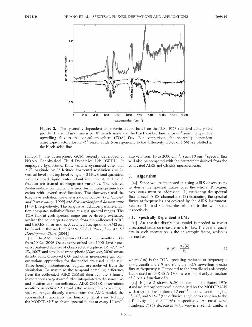
standard atmosphere profile computed by the MODTRAN5with a spectral resolution of 2 cm�1 for three zenith angles,0�, 60�, and 52.96� (the diffusive angle corresponding to thediffusivity factor of 1.66), respectively. At most wavenumbers, Rv(q) decreases with viewing zenith angle, a

Figure 2. The spectrally dependent anisotropic factors based on the U.S. 1976 standard atmosphereprofile. The solid gray line is for 0� zenith angle and the black dashed line is for 60� zenith angle. Theupwelling flux is the top-of-atmosphere (TOA) flux. For comparison, the spectrally dependentanisotropic factors for 52.96� zenith angle (corresponding to the diffusivity factor of 1.66) are plotted inthe black solid line.


4 of 16

D09110

dependence often referred to as ‘‘limb-darkening.’’ For allangles, the anisotropic factors in the atmospheric windowregions (850–1000 cm�1, 1100–1200 cm�1) and the watervapor pure rotational band (<500 cm�1) are closer to onethan those in other bands. The limb-darkening is stronger inthe ozone band (990–1070 cm�1), the Q-branch of methaneband (�1306 cm�1), and the water vapor v2 band (1200–2000 cm�1). In contrast, Rv(q) increases with viewing zenithangle in the center of the CO2 band (�667 cm�1),corresponding to ‘‘lime-brightening.’’ The contrast betweenthe CO2 band and other bands is primarily due to the factthat the effective emission levels for channels at the CO2

band center are located in the stratosphere rather than in thetroposphere. The larger the viewing zenith angle (q), thehigher the effective emission level. As temperatureincreases with the height in the stratosphere, this leads toa larger radiance intensity when q becomes larger. There-fore, if we define the frequency-dependent diffusive angle,qdiff, as pIv(qdiff) = Fv, then, for any q < qdiff, Rv(q) will besmaller than one; for any q > qdiff, Rv(q) will be larger thanone. In the troposphere, temperature decrease with thealtitude, which means that the opposite dependence ofRv(q) on q will occur.[17] As mentioned in section 2.1 and 2.2, necessary scene

type information can be retrieved from the CERES SSFproduct and then the scene type is directly applicable to thecollocated AIRS observation. According to Table 3 in thework of Loeb et al. [2005], clear-sky conditions over allsurface types are further stratified to 80 discrete intervals ofprecipitable water (pw), lapse rate (DT), and surface skintemperature (Ts). In practice, it turns out that only 14 out ofthe 80 intervals are needed to accommodate all possibleclear-sky scenes observed over the oceans, which are listedin detail in Table 1. Since we focus on tropical oceanregions in this study, we only need to construct appropriatespectral ADMs for the 14 intervals.[18] We use 6-hourly profiles from the ECMWF ERA-40

reanalysis [Uppala et al., 2005] in conjunction with theMODTRAN5 to derive the spectral ADMs for all 14intervals in the following way. Four months of ECMWFdata (October 2001, January 2002, April 2002, and July2002) are used. For each month, four 6-hourly time intervalsare chosen. For each selected 6-hourly period, temperature,

and humidity profiles between 60�S–60�N oceans are fedinto the MODTRAN5 to compute anisotropic factors ofindividual AIRS channels for zenith angles from 0� to 45�.By doing so, 80,640 profiles and associated synthetic AIRSspectra and anisotropic factors are archived. These profilesand anisotropic factors are then categorized into discreteintervals of pw, DT, and Ts as listed in Table 1. The meananisotropic factor from all samples belonging to a discreteinterval is defined as the anisotropic factor for that interval.By doing so, spectrally dependent ADMs for convertingAIRS radiances to spectra fluxes are constructed. Mean-while, broadband ADMs can also be obtained and checkedwith the CERES ADMs for consistency. For each discreteinterval, the CERES ADMs use a pair of slightly differentanisotropic factors (�0.1–0.4% difference in fraction), onefor the daytime scenes and the other for the nighttimescenes. Figure 3 shows a pair of such CERES anisotropicfactors for a given discrete interval (the gray solid lines withdiamonds and circles). The corresponding broadband an-isotropic factors derived from the aforementioned procedureare also shown in Figure 3 (black dash line). The threecurves closely follow each other with little differences. Thedifferences between the derived and the CERES daytimeanisotropic factor are �0.1%–0.2%. For the CERES night-time anisotropic factor, the differences range from �0.2% to�0.1%.

3.2. Estimating Spectral Fluxes at Frequencies NotCovered by AIRS

[19] In order to obtain spectral fluxes over the entirethermal-IR spectral range, a scheme has to be developedto estimate spectral fluxes at frequencies without the AIRScoverage. AIRS has no coverage at frequencies lower than649.6 cm�1 and between 1613.9 and 2000 cm�1. AIRS has

Table 1. The 14 Discrete Intervals of Precipitable Water (pw),

Lapse Rate (DT, Defined as the Vertical Temperature Change of

the First 300 hPa Above the Surface), and Surface Skin

Temperature (Ts) Used in the CERES LW ADMs to Determine

Clear-Sky OLR Over the Oceans

Discrete Interval pw(cm) DT(K) Ts (K)

1 0–1 <15 270–2902 0–1 <15 290–3103 0–1 15–30 270–2904 0–1 15–30 290–3105 1–3 <15 270–2906 1–3 <15 290–3107 1–3 15–30 270–2908 1–3 15–30 290–3109 1–3 15–30 310–33010 3–5 <15 270–29011 3–5 <15 290–31012 3–5 15–30 290–31013 >5 <15 290–31014 >5 15–30 290–310

Figure 3. The solid line with diamonds is LW broadbandanisotropic factor used in the CERES SSF product for thedaytime clear-sky scenes over the ocean with pw = 1–3 cm,DT < 15 K, and Ts = 290–310 K (discrete interval 6 inTable 1). The solid line with circles is used for thecorresponding nighttime clear-sky scenes. The thick dashedline is the LW broadband anisotropic factor derived fromthe procedure described in section 3.1.


5 of 16

D09110

12 modules assembled on the focal plane [Aumann et al.,2003], each having its own spectral range. The spectralranges of neighbor modules might overlap with each other.As a result, a few spectral ranges are sampled by more thanone module. Meanwhile, the modules do not provide acontinuous coverage from 649.6 cm�1 and 1613.9 cm�1.For example, no AIRS channel covers 1136.6–1217.0 cm�1

and 1046.2–1056.1 cm�1. To address the spectral coverageissue, the following strategy is adopted to cover the entirespectral range from 10 cm�1 to 2000 cm�1:[20] 1. For the spectral range continuously covered by

AIRS, AIRS channel frequency is used. For the spectralrange sampled by two overlapped channels, only onechannel is kept and used in later analysis.[21] 2. Frequency gaps between 649.6 cm�1 and

1613.9 cm�1 are covered with channels having the samespectral resolution as the nearest AIRS channels.[22] 3. For 10cm�1 to 649.6 cm�1, it is covered with

channels at a spectral resolution of 0.5 cm�1, approximatelythe same resolution as the nearest AIRS channel.[23] 4. For 1613.9 cm�1 to 2000cm�1, it is covered with

channels at a spectral resolution of 1.5 cm�1, approximatelythe same resolution as the nearest AIRS channel.[24] Hereafter, the above four sets of channels are referred

to as channel sets 1–4, respectively.[25] For AIRS channels in set 1, radiance Iv (q) can be

converted to the spectral flux Fv using the spectrallydependent ADMs described in section 3.1. For channelsin the sets of 2–4, a multiregression scheme based on thePrincipal Component Analysis is used to obtain thecorresponding spectra fluxes. Parameters in the regressionscheme are derived based on the ECMWF profiles andsynthetic spectra mentioned in section 3.1. For everyECMWF profile falling into a given discrete interval of(pw, DT, Ts), the synthetic spectral fluxes at all channels set1–4 are computed. Spectral EOF analysis (principal com-ponent analysis in the spectral domain) [Haskins et al.,1999; Huang et al., 2003; Huang and Yung, 2005] isapplied to the collection of synthetic spectral fluxes toderive a set of orthogonal basis in the frequency domain,

Fv ¼ �Fv þXNj¼1

ejfjv ð2Þ

where Fv is the synthetic spectral flux at frequency v fromone ECWMF profile and �Fv is the average of all syntheticspectral fluxes at v. N is the total number of channels, fv

j ( j =1�N) are the principal components (unit vectors) that consistof a complete set of orthogonal basis in the N-dimensionalspace, and ej is the projection of (Fv � �Fv) onto the jthprincipal component fv

j . In practice, it is found that 99.99%variance can be explained by the first 20 or even lessprincipal components. Therefore, we only retain the firstM principal components that account for 99.99% variance.In the matrix form, it means

F��F � f1;f2; . . . ;fM� �

e1e2. . .eM

2664

3775 ¼ Fe ð3Þ

where F, �F, f1, . . ., fI are vectors with a dimension ofN (N�M). Correspondingly, F is an NMmatrix and e isan M 1 vector. Note that the total number of channels inchannel sets 1–4 is N. The total number of AIRS channels(NAIRS) is smaller than N but much larger than M.[26] Since (3) holds for all channels, if we use AIRS in

subscript to denote a set of valid AIRS channels, we stillhave

FAIRS ��FAIRS � FAIRSe ð4Þ

[27] Note that FAIRS could be derived from AIRS mea-surement as described in section 3.1. �FAIRS, on the otherhand, are the mean spectral fluxes at the AIRS channels asderived from the set of synthetic spectra mentioned before.Equation (4) implies a least-square solution

e � FAIRSFAIRS

��1FAIRS FAIRS ��FAIRS

�ð5Þ

where F* is the transpose of F;. Once e is obtained forevery qualified AIRS observation, (3) can be used to derivethe spectral flux at each channel in sets 1–4, the channelsets not covered by the AIRS instrument. In practice,because of NAIRS � M, FAIRS is well-conditioned for everydiscrete intervals of (pw, DT, Ts) and inversion of (F*AIRSFAIRS) is numerically stable.[28] In summary, this method finds the least-square-fit of

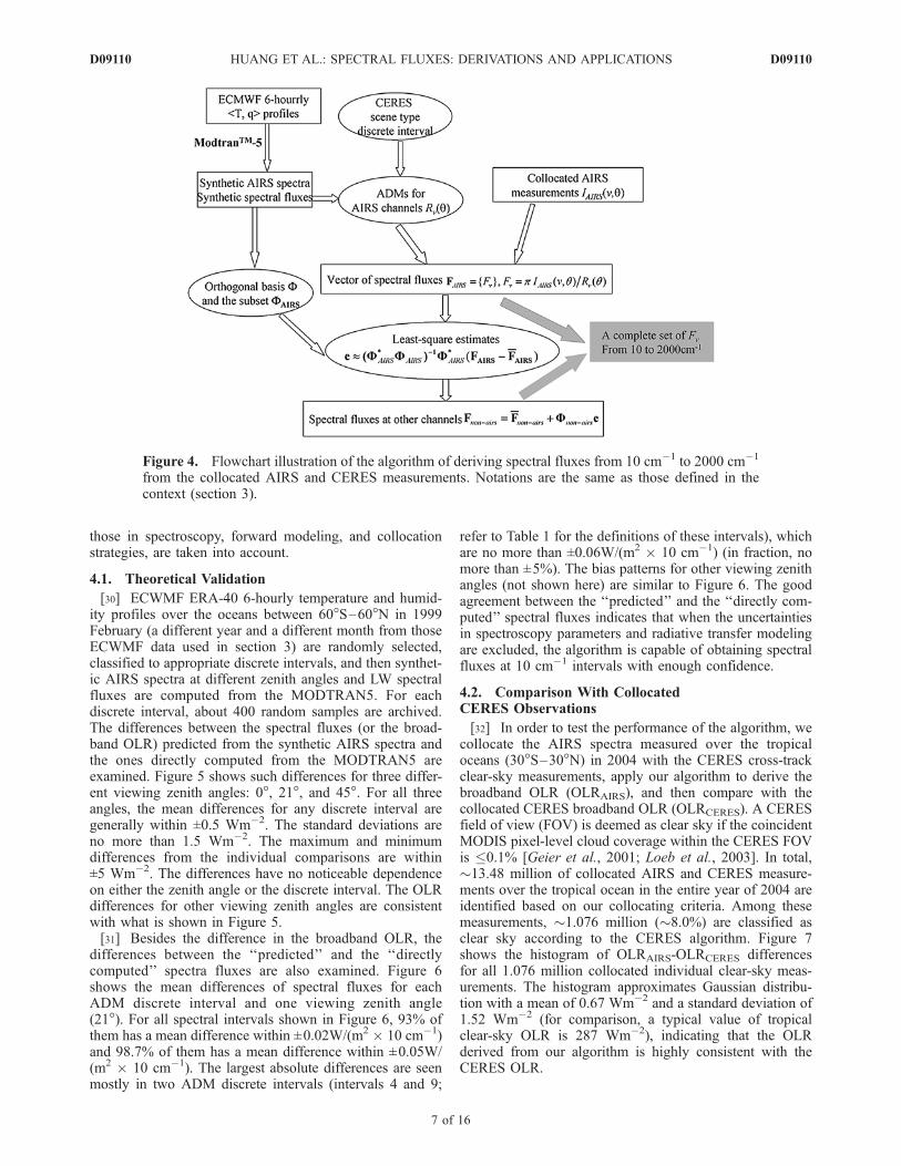
the projections of AIRS-derived spectral fluxes onto theprincipal components. Similar multivariate regression tech-nique has been used before to reconstruct global-scaletemperature patterns over the last six centuries [e.g., Mannet al., 1998]. While Mann et al. [1998] used this techniqueto fill missing spatial information, we used it here to fillmissing spectral information. In practice, an AIRS channelcould suffer from background electronic noise and, as aresult, it might provide meaningful observations most of thetime but could occasionally go wrong. This method is wellsuited for such situation since it only needs a subset ofAIRS channels with valid calibrated radiances. Thus, it cantolerate a varying set of qualified channels from measure-ment to measurement. It makes use of information from allavailable good channels yet avoids the painstaking errorhandling of bad channels for each individual measurement.A chart summarizing the whole algorithm described insection 3.1 and 3.2 is shown in Figure 4.

4. Validation

[29] Validating the algorithm described in section 3 isdone in two parts. The first part is ‘‘theoretical validation,’’synthetic AIRS spectra are used to derive the spectral fluxesand such spectral fluxes are compared with those directlycomputed from the MODTRAN5. The second part is usingthe algorithm to derive the broadband OLR from the AIRSspectrum and compare it with the collocated CERES OLR.The first part lets us assess the whole algorithm withoutconcerning the accuracy in spectroscopy and forward mod-eling since the MODTRAN5 is used as a surrogate ofradiative transfer in the real world. The second part is morerigorous in the sense that all realistic uncertainties, such as


6 of 16

D09110

those in spectroscopy, forward modeling, and collocationstrategies, are taken into account.

4.1. Theoretical Validation

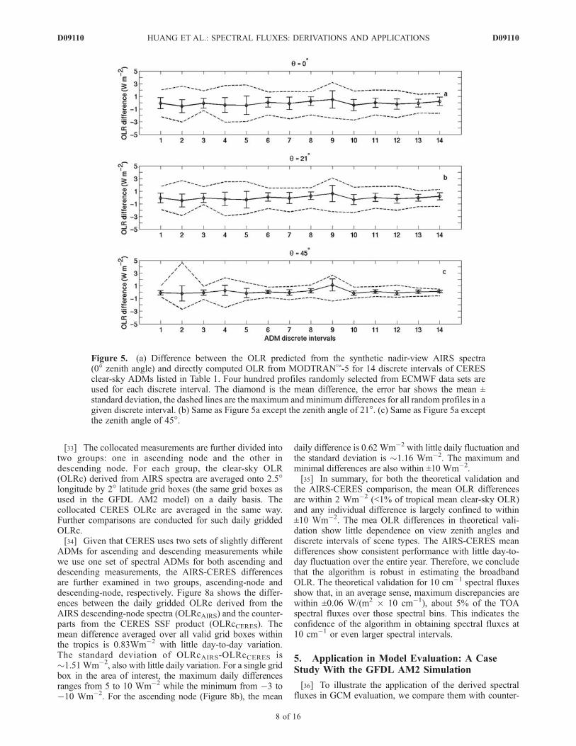
[30] ECWMF ERA-40 6-hourly temperature and humid-ity profiles over the oceans between 60�S–60�N in 1999February (a different year and a different month from thoseECWMF data used in section 3) are randomly selected,classified to appropriate discrete intervals, and then synthet-ic AIRS spectra at different zenith angles and LW spectralfluxes are computed from the MODTRAN5. For eachdiscrete interval, about 400 random samples are archived.The differences between the spectral fluxes (or the broad-band OLR) predicted from the synthetic AIRS spectra andthe ones directly computed from the MODTRAN5 areexamined. Figure 5 shows such differences for three differ-ent viewing zenith angles: 0�, 21�, and 45�. For all threeangles, the mean differences for any discrete interval aregenerally within ±0.5 Wm�2. The standard deviations areno more than 1.5 Wm�2. The maximum and minimumdifferences from the individual comparisons are within±5 Wm�2. The differences have no noticeable dependenceon either the zenith angle or the discrete interval. The OLRdifferences for other viewing zenith angles are consistentwith what is shown in Figure 5.[31] Besides the difference in the broadband OLR, the

differences between the ‘‘predicted’’ and the ‘‘directlycomputed’’ spectra fluxes are also examined. Figure 6shows the mean differences of spectral fluxes for eachADM discrete interval and one viewing zenith angle(21�). For all spectral intervals shown in Figure 6, 93% ofthem has a mean difference within ±0.02W/(m2 10 cm�1)and 98.7% of them has a mean difference within ±0.05W/(m2 10 cm�1). The largest absolute differences are seenmostly in two ADM discrete intervals (intervals 4 and 9;

refer to Table 1 for the definitions of these intervals), whichare no more than ±0.06W/(m2 10 cm�1) (in fraction, nomore than ±5%). The bias patterns for other viewing zenithangles (not shown here) are similar to Figure 6. The goodagreement between the ‘‘predicted’’ and the ‘‘directly com-puted’’ spectral fluxes indicates that when the uncertaintiesin spectroscopy parameters and radiative transfer modelingare excluded, the algorithm is capable of obtaining spectralfluxes at 10 cm�1 intervals with enough confidence.

4.2. Comparison With CollocatedCERES Observations

[32] In order to test the performance of the algorithm, wecollocate the AIRS spectra measured over the tropicaloceans (30�S–30�N) in 2004 with the CERES cross-trackclear-sky measurements, apply our algorithm to derive thebroadband OLR (OLRAIRS), and then compare with thecollocated CERES broadband OLR (OLRCERES). A CERESfield of view (FOV) is deemed as clear sky if the coincidentMODIS pixel-level cloud coverage within the CERES FOVis �0.1% [Geier et al., 2001; Loeb et al., 2003]. In total,�13.48 million of collocated AIRS and CERES measure-ments over the tropical ocean in the entire year of 2004 areidentified based on our collocating criteria. Among thesemeasurements, �1.076 million (�8.0%) are classified asclear sky according to the CERES algorithm. Figure 7shows the histogram of OLRAIRS-OLRCERES differencesfor all 1.076 million collocated individual clear-sky meas-urements. The histogram approximates Gaussian distribu-tion with a mean of 0.67 Wm�2 and a standard deviation of1.52 Wm�2 (for comparison, a typical value of tropicalclear-sky OLR is 287 Wm�2), indicating that the OLRderived from our algorithm is highly consistent with theCERES OLR.

Figure 4. Flowchart illustration of the algorithm of deriving spectral fluxes from 10 cm�1 to 2000 cm�1

from the collocated AIRS and CERES measurements. Notations are the same as those defined in thecontext (section 3).


7 of 16

D09110

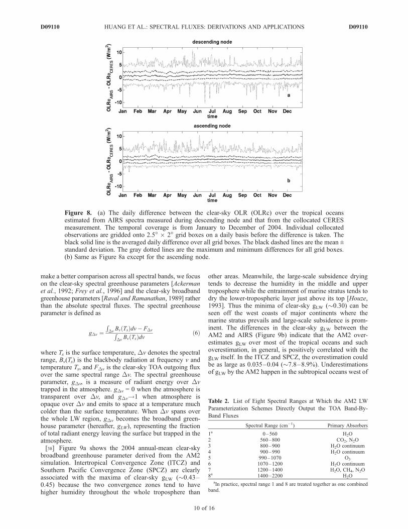
[33] The collocated measurements are further divided intotwo groups: one in ascending node and the other indescending node. For each group, the clear-sky OLR(OLRc) derived from AIRS spectra are averaged onto 2.5�longitude by 2� latitude grid boxes (the same grid boxes asused in the GFDL AM2 model) on a daily basis. Thecollocated CERES OLRc are averaged in the same way.Further comparisons are conducted for such daily griddedOLRc.[34] Given that CERES uses two sets of slightly different

ADMs for ascending and descending measurements whilewe use one set of spectral ADMs for both ascending anddescending measurements, the AIRS-CERES differencesare further examined in two groups, ascending-node anddescending-node, respectively. Figure 8a shows the differ-ences between the daily gridded OLRc derived from theAIRS descending-node spectra (OLRcAIRS) and the counter-parts from the CERES SSF product (OLRcCERES). Themean difference averaged over all valid grid boxes withinthe tropics is 0.83Wm�2 with little day-to-day variation.The standard deviation of OLRcAIRS-OLRcCERES is�1.51 Wm�2, also with little daily variation. For a single gridbox in the area of interest, the maximum daily differencesranges from 5 to 10 Wm�2 while the minimum from �3 to�10 Wm�2. For the ascending node (Figure 8b), the mean

daily difference is 0.62 Wm�2 with little daily fluctuation andthe standard deviation is �1.16 Wm�2. The maximum andminimal differences are also within ±10 Wm�2.[35] In summary, for both the theoretical validation and

the AIRS-CERES comparison, the mean OLR differencesare within 2 Wm�2 (<1% of tropical mean clear-sky OLR)and any individual difference is largely confined to within±10 Wm�2. The mea OLR differences in theoretical vali-dation show little dependence on view zenith angles anddiscrete intervals of scene types. The AIRS-CERES meandifferences show consistent performance with little day-to-day fluctuation over the entire year. Therefore, we concludethat the algorithm is robust in estimating the broadbandOLR. The theoretical validation for 10 cm�1 spectral fluxesshow that, in an average sense, maximum discrepancies arewithin ±0.06 W/(m2 10 cm�1), about 5% of the TOAspectral fluxes over those spectral bins. This indicates theconfidence of the algorithm in obtaining spectral fluxes at10 cm�1 or even larger spectral intervals.

5. Application in Model Evaluation: A CaseStudy With the GFDL AM2 Simulation

[36] To illustrate the application of the derived spectralfluxes in GCM evaluation, we compare them with counter-

Figure 5. (a) Difference between the OLR predicted from the synthetic nadir-view AIRS spectra(0� zenith angle) and directly computed OLR from MODTRAN

TM

-5 for 14 discrete intervals of CERESclear-sky ADMs listed in Table 1. Four hundred profiles randomly selected from ECMWF data sets areused for each discrete interval. The diamond is the mean difference, the error bar shows the mean ±standard deviation, the dashed lines are the maximum and minimum differences for all random profiles in agiven discrete interval. (b) Same as Figure 5a except the zenith angle of 21�. (c) Same as Figure 5a exceptthe zenith angle of 45�.


8 of 16

D09110

parts from the AM2 model simulation over the same periodas forced by observed sea surface temperature (SST). Asmentioned in section 2, the output of AM2 simulation isfurther sampled to ensure consistent temporal and spatialsampling patterns with the observations. All comparisonsare based on such a subsampled AM2 data set. Forsimplicity, all comparisons are done with data collectedduring the ascending node only. Similar conclusions can bereached when the descending data are examined. Occasion-ally, in order to contrast the differences between the AM2model and observations, 6-hourly NCEP-DOE reanalysisdata [Kanamitsu et al., 2002] for the year of 2004 is used togenerate a ‘‘third-party’’ comparison. The 6-hourly NCEP-DOE reanalysis data is processed in the same way as theAM2 model output and corresponding synthetic spectralfluxes are computed from the MODTRAN5. Section 5.1focuses on the band-by-band IR fluxes directly output fromthe AM2. Section 5.2 discusses the comparison at a finerspectral resolution, 10 cm�1 spectral interval.

5.1. Band-By-Band IR Fluxes

[37] The AM2 LW radiation parameterization schemeoutputs the LW fluxes over eight different spectral ranges(bands) as listed in Table 2. In practice, two of them (0–560 cm�1, 1400–2200 cm�1) are treated together as acombined band. The absolute flux can vary by a factor upto 10 from one band to another band used in the AM2. To

Figure 6. The mean difference between the predicted TOA spectra fluxes based on synthetic AIRSspectra and the directly computed TOA spectral fluxes from MODTRAN

TM

-5 for each ADM discreteinterval. The spectral flux is computed for every 10 cm�1 interval from 10 to 2000 cm�1. Ordinaterepresents the 14 discrete intervals of CERES clear-sky ADMs listed in Table 1. Four hundred profilesrandomly selected from ECMWF data sets are used to calculate the mean difference for each discreteinterval. The unit of the mean difference is W per m2 per 10 cm�1.

Figure 7. Histogram of differences between AIRS-derivedOLR and CERES OLR for all individually collocated AIRSand CERES clear-sky footprints over the tropical oceans in2004. In total 1.076 million collocated footprints areidentified. The mean is 0.67 Wm�2 and the standarddeviation is 1.52 Wm�2.


9 of 16

D09110

make a better comparison across all spectral bands, we focuson the clear-sky spectral greenhouse parameters [Ackermanet al., 1992; Frey et al., 1996] and the clear-sky broadbandgreenhouse parameters [Raval and Ramanathan, 1989] ratherthan the absolute spectral fluxes. The spectral greenhouseparameter is defined as

gDv ¼RDv

Bv Tsð Þdv� FDvRDv

Bv Tsð Þdv ð6Þ

where Ts is the surface temperature, Dv denotes the spectralrange, Bv(Ts) is the blackbody radiation at frequency v andtemperature Ts, and FDv is the clear-sky TOA outgoing fluxover the same spectral range Dv. The spectral greenhouseparameter, gDv, is a measure of radiant energy over Dvtrapped in the atmosphere. gDv = 0 when the atmosphere istransparent over Dv, and gDv!1 when atmosphere isopaque over Dv and emits to space at a temperature muchcolder than the surface temperature. When Dv spans overthe whole LW region, gDv becomes the broadband green-house parameter (hereafter, gLW), representing the fractionof total radiant energy leaving the surface but trapped in theatmosphere.[38] Figure 9a shows the 2004 annual-mean clear-sky

broadband greenhouse parameter derived from the AM2simulation. Intertropical Convergence Zone (ITCZ) andSouthern Pacific Convergence Zone (SPCZ) are clearlyassociated with the maxima of clear-sky gLW (�0.43–0.45) because the two convergence zones tend to havehigher humidity throughout the whole troposphere than

other areas. Meanwhile, the large-scale subsidence dryingtends to decrease the humidity in the middle and uppertroposphere while the entrainment of marine stratus tends todry the lower-tropospheric layer just above its top [Houze,1993]. Thus the minima of clear-sky gLW (�0.30) can beseen off the west coasts of major continents where themarine stratus prevails and large-scale subsidence is prom-inent. The differences in the clear-sky gLW between theAM2 and AIRS (Figure 9b) indicate that the AM2 over-estimates gLW over most of the tropical oceans and suchoverestimation, in general, is positively correlated with thegLW itself. In the ITCZ and SPCZ, the overestimation couldbe as large as 0.035–0.04 (�7.8–8.9%). Underestimationsof gLW by the AM2 happen in the subtropical oceans west of

Figure 8. (a) The daily difference between the clear-sky OLR (OLRc) over the tropical oceansestimated from AIRS spectra measured during descending node and that from the collocated CERESmeasurement. The temporal coverage is from January to December of 2004. Individual collocatedobservations are gridded onto 2.5� 2� grid boxes on a daily basis before the difference is taken. Theblack solid line is the averaged daily difference over all grid boxes. The black dashed lines are the mean ±standard deviation. The gray dotted lines are the maximum and minimum differences for all grid boxes.(b) Same as Figure 8a except for the ascending node.

Table 2. List of Eight Spectral Ranges at Which the AM2 LW

Parameterization Schemes Directly Output the TOA Band-By-

Band Fluxes

Spectral Range (cm�1) Primary Absorbers

1a 0–560 H2O2 560–800 CO2, N2O3 800–900 H2O continuum4 900–990 H2O continuum5 990–1070 O3

6 1070–1200 H2O continuum7 1200–1400 H2O, CH4, N2O8a 1400–2200 H2O

aIn practice, spectral range 1 and 8 are treated together as one combinedband.


10 of 16

D09110

major continents and the central and eastern Pacific (90–180�W) in the deep tropics, regions featured with large-scale subsidence. As we shall see later, such overestimationsand underestimations in the broadband gLW have in factoriginated from different spectral ranges.[39] Figure 9c shows the simulated annual-mean clear-

sky spectral greenhouse parameters (hereafter, gDv) over thecombined band of 0–560 cm�1 and 1400–2200 cm�1

(hereafter, the combined water vapor band). Both 0–560 cm�1 and 1400–2200 cm�1 bands are sensitive torelative humidity over a broad vertical layer approximatelyfrom 600 hPa to 200 hPa. As a result, the gDv is highlycorrelated with the water vapor amount in the middle andupper troposphere, with maxima over the ITCZ and SPCZand minima over the large-scale subsidence regions. Thecorresponding AM2-AIRS difference shown in Figure 9d ispositive over all of the tropical oceans. This suggests that

the AM2 overestimates the relative humidity in the middleand upper troposphere for the entire tropical oceans. Wenote here that satellite only samples the clear-sky footprintswhile the model output, even subsampled according to thesatellite tracks, could be cloudy profiles. Therefore, suchsampling difference might partly explain the differencesseen in Figure 9d, especially over the convective regions.Huang et al. [2006] examined the same model and showedthat the majority of model bias cannot be explained by suchsampling difference alone. The gDv in the window region(Figure 9e) is much smaller than both the gLW and the gDv ofthe combined water vapor band: the AM2-simulated gDv isonly �0.12–0.15 in the ITCZ and SPCZ and �0.04 in theother tropical oceans. This is because, besides the watervapor continuum absorption, the atmosphere is almosttransparent in the window region. The water vapor contin-uum absorption in this spectral region is proportional to the

Figure 9. (a) The 2004 annual-mean broadband greenhouse parameters (gLW) over the tropical oceanssimulated by the AM2. (b) The difference between AM2-simulated and AIRS-inferred gLW. (c)–(d) Sameas Figures 9a–9b except for the spectral greenhouse parameters over the combined band of 0–560 cm�1

and 1400–2200 cm�1. (e)–(f) and (g)–(h) Same as Figures 9c–9d except for spectral ranges of 560–800 cm�1 and 990–1070 cm�1, respectively. Please note four different color bars, corresponding to fourdifferent sets of value range, are used here.


11 of 16

D09110

square of water vapor concentration, which makes it mostsensitive to the water vapor concentration from the surfaceto �3 km. The AM2-AIRS difference over this spectralrange (Figure 9f) indicates an overestimation of �0.02–0.04 in the large-scale convergence zones. In the large-scalesubsidence regions, especially the oceans west of majorcontinents, gDv is underestimated by �0.01–0.02. Samegeographical patterns of the AM2-AIRS differences can beseen in other window regions as well (800–900 cm�1,1070–1200 cm�1, not shown here). Such differences sug-gest an overestimation of the lower tropospheric (0–3 km)humidity in the large-scale convergence zones and anunderestimation of it in the large-scale subsidence regionsby the AM2. In the large-scale subsidence regions, theunderestimation over the window regions (e.g., Figure 9f)slightly outplays the overestimation over the combinedwater vapor bands (Figure 9d) and other spectral ranges.As a result, the AM2 broadband gLW at these regions areslightly underestimated (Figure 9b). For the large-scaleconvergence zones, overestimations exist in both the watervapor bands and the window regions, which leads to a�10% overestimation in the AM2 broadband gLW.[40] Figure 9g shows the simulated gDv for the spectral

range of 990–1070 cm�1 (the ozone band). Unlike otherspectral ranges discussed above, the simulated gDv of thisspectral range has maxima in the subtropics rather than inthe deep tropics because of the higher lower stratosphericozone concentrations in the subtropics in comparison to thedeep tropics. The AM2-AIRS differences (Figure 9h) showa zonally uniform pattern with minima in the deep tropics.

Given the AM2 simulation is done with the 1990s ozoneclimatology, the AM2-AIRS differences here reflect (1) thedifference of ozone distribution between the 1990s clima-tology used in the simulation and the actual ozone distri-bution in 2004 and (2) the lower stratospheric temperaturedifference between the AM2 simulation and the reality.

5.2. Comparisons of 10 cm�1 Spectral Fluxes

[41] When comparisons are conducted in a finer spectralresolution, 10 cm�1 spectral interval, further compensatingdifferences within a given band can be revealed. Figure 10ashows the annual-mean clear-sky spectral fluxes averagedover tropical oceans for every 10 cm�1 interval from10 cm�1 to 2000 cm�1 as computed from the MODTRAN5based on the AM2 output (the solid line) and as derivedfrom collocated AIRS and CERES observations (the dashedline). The corresponding AM2-AIRS difference is shown inFigure 10c. The corresponding annual-mean spectral green-house parameters are shown in Figure 10b and their differ-ences in Figure 10d. The spectral flux difference from 10 to300 cm�1 is close to zero, followed by systematic negativedifference in the rest of water vapor rotational band (300–560 cm�1). Correspondingly, the AM2-AIRS difference ingDv is positive from 300 to 560 cm�1. The water vapor v2band (�1200–2000 cm�1) has the highest gDv (�0.6–0.85) among all spectral ranges and the difference in gDv

is also systematically positive. CO2 667 cm�1 band showscompensating errors from the different parts of the band: theflux (gDv) differences in the band center are positive(negative) while those in the band wings are negative

Figure 10. (a) The annual-mean clear-sky spectral flux (per 10 cm�1 intervals) over the tropical oceansas inferred from the AIRS and CERES collocated observations (dashed line) and simulated fromMODTRAN5 based on the AM2 6-hourly output (solid line). (b) Same as Figure 10a except for annual-mean clear-sky spectral greenhouse parameters (gDv) at 10 cm�1 intervals. The annual-mean gDv isderived from 12 monthly means of gDv. (c) The differences between the AM2-simulated and the AIRS-inferred spectra fluxes shown in Figure 10a. (d) The differences between the AM2 and AIRS gDv shownin Figure 10b. The dotted gray lines indicate the start and ending frequencies of the portion of AIRSspectrum used in this study.


12 of 16

D09110

(positive), indicating that the biases of the AM2-simulatedtropospheric and stratospheric temperatures have oppositesigns.[42] Besides the annual mean gDv, monthly variations

from the annual mean can be examined to reveal theseasonal cycle of gDv. Such monthly anomalies are shownin Figure 11a and 11b for the AM2 and observations,respectively. For the window regions, both the AM2 andobservations show positive variations (compared to theannual mean) from January to June with maxima in Apriland negative anomalies in the other months with minima inAugust. For part of the water vapor rotational bands (300–560 cm�1) and the whole water vapor v2 band, both theAM2 and observations have maximum positive variations inApril. However, the observed negative anomalies over thesame spectral regions peak in August while the simulatedones tend to have broad negative minima extended fromAugust to October and even to December. For comparison,6-hourly NCEP-DOE reanalysis (NCEP-II) data over the

same period is processed in the same way as the AM2model output and the corresponding monthly variations ofgDv are shown in Figure 11c. For NCEP-II reanalysis, thenegative minima in the water vapor bands are concentratedin October, different from both the AM2 simulation and theAIRS-inferred observations. This reflects differences insimulated, assimilated, and observed seasonality of tropicalmiddle and upper troposphere relative humidity, especiallyin the second half year. The AM2, AIRS, and NCEP-II allreveal prominent seasonal variations of gDv around the CO2

band center (640–690 cm�1) but the peaks in the AM2 lagthose in the observations by 1–2 months, suggesting thediscrepancies in simulating the phase of seasonal variationsin the middle and lower stratospheric temperature. TheNCEP-II, on the other hand, agrees with the AIRS to alarge extent for both the phase and amplitude of the seasonalvariations in the CO2 band center. The AIRS exhibit astrong seasonal variation in the O3 band center (1010–1065 cm�1) with maximum in July–September and mini-

Figure 11. (a) The AM2 monthly variations of the clear-sky spectral greenhouse parameters gDv

(per 10 cm�1 interval) from the annual mean gDv (the solid line in Figure 9b) as computed fromMODTRAN

TM

-5. (b) Same as Figure 11a except for the gDv derived from collocated AIRS and CERESobservations. (c) Same as Figure 11a except for the 2004 NCEP-DOE reanalysis 6-hourly output. The6-hourly NCEP-DOE reanalysis is processed in a way similar to the AM2 output. The dash gray linesindicate the start and ending frequencies of the portion of AIRS spectrum used in this study.


13 of 16

D09110

mum in January–March. This seasonal variation is primar-ily due to seasonal changes of ozone concentration becausewhen a constant tropical-mean ozone profile is used in theMODTRAN5 for generating all synthetic spectral fluxes forboth the AM2 and NCEP-II, such seasonal variations in theozone band are hardly seen (Figure 11a and 11c).[43] Sections 5.1 and 5.2 demonstrate that the spectral

fluxes derived from the collocated AIRS and CERES datacan be used to evaluate climate models in various ways. Theband-by-band fluxes calculated in the GCM can be directlycompared with the derived spectral fluxes. Compensatingerrors among different bands can be disclosed in this way.Also, using a narrow-band radiative transfer model like theMODTRAN5, comparison could be done at even finerspectral resolution and compensating errors within an indi-vidual band can be further revealed.

6. Conclusions and Discussions

[44] Collocated AIRS and CERES observations are usedin this study to derive clear-sky outgoing spectral fluxes at10 cm�1 interval from 10 to 2000 cm�1. The spectralADMs are developed based on the CERES scene types.Such ADMs are then used to convert the AIRS radiances tospectral fluxes. Fluxes over the spectral ranges not coveredby the AIRS instrument are derived using a multivariateregression scheme. The algorithm is validated against syn-thetic spectral fluxes as well as the collocated CERESbroadband OLR.[45] Using the GFDL AM2 model as a case study,

applications of the derived clear-sky spectral fluxes inGCM evaluations are also discussed. Such spectral fluxescan reveal the compensating errors that cannot be detectedin the traditional comparison of the broadband OLR. Com-pensating errors from different broad spectral ranges as wellas within a given spectral range can be quantitativelyrevealed. The comparisons with the AM2 simulation showhow the spatial distribution and temporal evolution of watervapor at different parts of the troposphere contribute to thespectral flux differences. As shown in Figure 9, the AM2tends to be more humid than the observations in the middleand upper troposphere for all tropical oceans. In the lowertroposphere, it tends to be more humid in the large-scaleconvergence zones but dryer in the large-scale subsidencezones. This suggests dynamical causes of simulated watervapor biases. As for the seasonal variations of the spectralfluxes in the water vapor rotational band and v2 band, theAM2 model agrees with the AIRS observation and NCEP-IIreanalysis for the first half year but not for the second halfyear: the AM2 model has broad negative variations span-ning from August to October and even to December whilethe AIRS shows negative minima concentrated in Augustand the NCPE-II data has negative minima in October. Suchdiscrepancies among model, observation, and reanalysis inthe spectral domain confirm the value of infrared spectralfluxes in model evaluation.[46] This study serves as the first step toward deriving the

TOA spectral cloud radiative forcing. While temperatureand humidity profiles retrieved from AIRS spectra can beused to compute the TOA clear-sky spectral fluxes, tocompute TOA cloudy spectral fluxes from retrieval productsis subject to more uncertainties because of the difficulty of

reliably retrieving cloud properties from IR sounders. Withan ultimate goal of deriving TOA spectral cloud radiativeforcing, we choose to work directly with radiance measure-ments so the CERES-like methodology can be applied toboth clear-sky and cloudy measurements consistently.Besides, AIRS retrieved temperature and humidity profilesare the averaged quantities over 3 3 AIRS footprints,which might bring additional difficulty when the OLRcomputed from such retrievals is to be compared withcollocated CERES OLR at the single FOV level.[47] Meanwhile, we acknowledge that in principle AIRS

level-2 retrieval products alone can be used to computespectral fluxes [Mehta and Susskind, 1999] independentlyand it has its own uniqueness [Susskind et al., 2003; Molnarand Susskind, 2006]. The concept of effective zenith angleintroduced by Mehta and Susskind [1999] makes it possibleto compute spectral fluxes from retrieval products in aneconomical way. AIRS retrieval adopts a cloud-clearingapproach [Susskind et al., 2003]. As a result, the clear-skyflux computed from such retrieval products represents theflux that would have gone to space if the scene wereotherwise identical but cloud free, which is consistent withthe definition of clear-sky flux computed from the climatemodels. To fully investigate the application of AIRS level-2retrieval products in deriving band-by-band flux and spec-tral cloud radiative forcing is beyond the scope of this studysince the focus here is a radiance-to-flux approach andcollocation with CERES is desired for ensuring the validityof this approach.[48] The confidence in the spectral fluxes derived from

the collocated AIRS and CERES observations depends onthe accuracy of the algorithm described in section 3.Uncertainties in the derived spectral fluxes could originatefrom various sources. The mean spectral fluxes and thecorresponding principal components used in the multivari-ate regression schemes have their limitations since they arederived from a set of finite samples. Another source of errorexists in the forward radiative transfer modeling, MOD-TRAN5, especially in the far IR, a spectral range notcovered by the AIRS instrument and therefore purelyrelying on the MODTRAN5 and the regression scheme.The importance of far-IR water vapor absorption to theclear-sky radiative budget has been long recognized[Clough et al., 1992; Sinha and Harries, 1995, 1997]. Thisstudy has to infer the far-IR spectral fluxes since AIRS hasno coverage in the far IR. Such inferences are feasiblebecause of the redundant information content between thewater vapor rotation band and the water vapor v2 band, thelatter being largely covered by the AIRS instrument. To alarge extent, the regression scheme infers the far-IR spectrafluxes through the close correlations between the two watervapor bands. With more investigative efforts on directlyobserving spectrally resolved radiance in the far IR fromspace [Mlynczak et al., 2006; Palchetti et al., 2006], thissituation could be improved in the future by mergingobservations from multiple spectrometer instruments tocreate a merged data set of spectral fluxes over the entirethermal-IR spectral range.

[49] Acknowledgments. The AIRS data were obtained from NASAGSFC DAAC and the CERES data from NASA Langley DAAC. TheNCEP-DOS reanalysis data were obtained from http://www.cdc.noaa.gov.


14 of 16

D09110

The ECMWF reanalysis data were obtained from http://data.ecmwf.int/data/d/era40_daily/. We thank R. Hemler, Y. Huang, E. Fetzer, E. Fishbein, S.Y.Lee, and S. Leroy for valuable discussion and help. One of the authors,Wenze Yang, was supported by a University of Michigan internal fund. Wealso wish to thank two anonymous reviewers for improving the quality ofthis paper.

ReferencesAckerman, S. A., et al. (1992), Radiation budget studies using collocatedobservations from Advanced Very High-Resolution Radiometer, High-Resolution Infrared Sounder/2, and Earth Radiation Budget Experimentinstruments, J. Geophys. Res., 97, 11,513–11,525.

Allan, R. P., et al. (2004), Simulation of the Earth’s radiation budget by theEuropean centre for Medium-Range Weather Forecasts 40-year reanalysis(ERA40), J. Geophys. Res., 109, D18107, doi:10.1029/2004JD004816.

Anderson, G., et al. (2006), Atmospheric sensitivity to spectral top-of-atmo-sphere solar irradiance perturbations, using MODTRAN-5 radiativetransfer algorithm, Eos Trans. AGU, 87(52), Fall Meet. Suppl., AbstractA11C-05.

Aumann, H. H., et al. (2003), AIRS/AMSU/HSB on the aqua mission:Design, science objectives, data products, and processing systems, IEEETrans. Geosci. Remote Sens., 41, 253–264, doi:10.1109/TGRS.2002.808356.

Barkstrom, B. R. (1984), The Earth Radiation Budget Experiment (ERBE),Bull. Am. Meteorol. Soc., 65, 1170 – 1185, doi:10.1175/1520-0477(1984)065<1170:TERBE>.

Berk, A., et al. (1998), MODTRAN cloud and multiple scattering upgradeswith application to AVIRIS, Remote Sens. Environ., 65, 367 –375,doi:10.1016/S0034-4257(98)00045-5.

Berk, A., et al. (2005), MODTRAN5: A reformulated atmospheric bandmodel with auxiliary species and practical multiple scattering options,Proc. SPIE Int. Soc. Opt. Eng., 5655, 88.

Bernstein, L. S., et al. (1996), Very narrow band model calculations ofatmospheric fluxes and cooling rates, J. Atmos. Sci., 53, 2887–2904,doi:10.1175/1520-0469(1996)053<2887:VNBMCO>.

Chahine, M. T., et al. (2006), AIRS: Improving weather forecasting andproviding new data on greenhouse gases, Bull. Am. Meteorol. Soc., 87,911–926, doi:10.1175/BAMS-87-7-911.

Clough, S. A., and M. J. Iacono (1995), Line-by-line calculation of atmo-spheric fluxes and cooling rates: 2. Application to carbon dioxide, ozone,methane, nitrous oxide and the halocarbons, J. Geophys. Res., 100,16,519–16,535, doi:10.1029/95JD01386.

Clough, S. A., et al. (1992), Line-by-line calculations of atmospheric fluxesand cooling rates: Application to water vapor, J. Geophys. Res., 97,15,761–15,785.

Clough, S. A., et al. (2005), Atmospheric radiative transfer modeling: Asummary of the AER codes, J. Quant. Spectrosc. Radiat. Transf., 91,233–244, doi:10.1016/j.jqsrt.2004.05.058.

DAO (1996), Algorithm Theoretical Basis Document for Goddard EarthObserving System Data Assimilation System (GOES DAS) With a FocusVersion 2, 310 pp., Data Assimilation Off., NASA Goddard Space FlightCent., Greenbelt, Md.

Feldman, D. R., et al. (2006), Direct retrieval of stratospheric CO2 infraredcooling rate profiles from AIRS data, Geophys. Res. Lett., 33, L11803,doi:10.1029/2005GL024680.

Freidenreich, S. M., and V. Ramaswamy (1999), A new multiple-band solarradiative parameterization for general circulation models, J. Geophys.Res., 104, 31,389–31,409, doi:10.1029/1999JD900456.

Frey, R. A., et al. (1996), Climate parameters from satellite spectral mea-surements. 1. Collocated AVHRR and HIRS/2 observations of spectralgreenhouse parameter, J. Clim., 9, 327–344, doi:10.1175/1520-0442(1996)009<0327:CPFSSM>2.0.CO;2.

Gaiser, S. L., et al. (2003), In-flight spectral calibration of the atmosphericinfrared sounder, IEEE Trans. Geosci. Rem. Sens., 41, 287 – 297,doi:10.1109/TGRS.2003.809708.

Geier, E. B., et al. (2001), Single Satellite Footprint TOA/Surface Fluxesand Clouds (SSF) Collection Documents, 243 pp., Clim. Sci. Branch,NASA Langley Res. Cent., Hampton, Va. (Available at http://asd-www.larc.nasa.gov/ceres/collect_guide/SSF-CG.pdf)

GFDL Global Atmosphere Model Development Team (2004), The newGFDL global atmosphere and land model AM2–LM2: Evaluation withprescribed SST simulations, J. Clim., 17, 4641–4673, doi:10.1175/JCLI-3223.1.

Goodberlet, M. A., et al. (1990), Ocean surface wind-speed measurementsof the Special Sensor Microwave Imager (SSM/I), IEEE Trans. Geosci.Remote Sens., 28, 823–828, doi:10.1109/36.58969.

Goody, R., et al. (1998), Testing climate models: An approach, Bull. Am.Meteorol. Soc., 79, 2541–2549, doi:10.1175/1520-0477(1998)079<2541:TCMAA>2.0.CO;2.

Harries, J. E., et al. (2005), The Geostationary Earth Radiation Budget(GERB) project, Bull. Am. Meteorol. Soc., 86, 945–960, doi:10.1175/BAMS-86-7-945.

Haskins, R., et al. (1999), Radiance covariance and climate models, J. Clim.,12, 1409–1422, doi:10.1175/1520-0442(1999)012<1409:RCACM>2.0.CO;2.

Horowitz, L. W. (2006), Past, present, and future concentrations of tropo-spheric ozone and aerosols: Methodology, ozone evaluation, and sensi-tivity to aerosol wet removal, J. Geophys. Res., 111, D22211,doi:10.1029/2005JD006937.

Houze, R. A. (1993), Cloud Dynamics, 573 pp., Elsevier, New York.Huang, X. L., and Y. L. Yung (2005), Spatial and spectral variability ofthe outgoing thermal IR spectra from AIRS: A case study of July 2003,J. Geophys. Res., 110, D12102, doi:10.1029/2004JD005530.

Huang, X. L., J. J. Liu, and Y. L. Yung (2003), Analysis of thermal emis-sion spectrometer data using spectral EOF and tri-spectral methods,Icarus, 165, 301–314, doi:10.1016/S0019-1035(03)00206-9.

Huang, X. L., V. Ramaswamy, and M. D. Schwarzkopf (2006), Quantifica-tion of the source of errors in AM2 simulated tropical clear-sky outgoinglongwave radiation, J. Geophys. Res., 111, D14107, doi:10.1029/2005JD006576.

Huang, Y., V. Ramaswamy, X. L. Huang, Q. Fu, and C. Bardeen (2007), Astrict test in climate modeling with spectrally resolved radiances: GCMsimulation versus AIRS observations, Geophys. Res. Lett., 34, L24707,doi:10.1029/2007GL031409.

Kanamitsu, M., et al. (2002), NCEP-DOEAMIP-II reanalysis (R-2), Bull. Am.Meteorol. Soc., 83, 1631–1643, doi:10.1175/BAMS-83-11-1631(2002)083<1631:NAR>2.3.CO;2.

Loeb, N. G., et al. (2001), Determination of unfiltered radiances fromthe clouds and the Earth’s Radiant Energy System instrument, J. Appl.Meteorol., 40, 822 – 835, doi:10.1175/1520-0450(2001)040<0822:DOURFT>2.0.CO;2.

Loeb, N. G., et al. (2003), Angular distribution models for top-of-atmosphere radiative flux estimation from the clouds and the Earth’sRadiant Energy System instrument on the Tropical Rainfall MeasuringMission satellite. part I: Methodology, J. Appl. Meteorol., 42, 240–265,doi:10.1175/1520-0450(2003)042<0240:ADMFTO>2.0.CO;2.

Loeb, N. G., et al. (2005), Angular distribution models for top-of-atmosphere radiative flux estimation from the Clouds and the Earth’sRadiant Energy System instrument on the Terra satellite. Part I: Methodol-ogy, J. Atmos. Ocean. Technol., 22, 338–351, doi:10.1175/JTECH1712.1.

Loeb, N. G., et al. (2007), Angular distribution models for top-of-atmosphere radiative flux estimation from the Clouds and the Earth’sRadiant Energy System instrument on the Terra satellite. Part II: Validation,J. Atmos. Ocean. Technol., 24, 564–584, doi:10.1175/JTECH1983.1.

Mann, M. E., R. S. Bradley, and M. K. Hughes (1998), Global-scale tem-perature patterns and climate forcing over the past six centuries, Nature,392, 779–787, doi:10.1038/33859.

Mehta, A., and J. Susskind (1999), Outgoing longwave radiation from theTOVS Pathfinder Path A data set, J. Geophys. Res., 104(D10), 12,193–12,212, doi:10.1029/1999JD900059.

Mlynczak, M. G., et al. (2006), First light from the Far-Infrared Spectro-scopy of the Troposphere (FIRST) instrument, Geophys. Res. Lett., 33,L07704, doi:10.1029/2005GL025114.

Molnar, G. I., and J. Susskind (2006), Satellite sounder-based OLR-,cloud- and atmospheric temperature climatologies for climate analyses,in Algorithms and Technologies for Multispectral, Hysperspectral, andUltraspectral Imagery XII, edited by S. S. Shen and P. E. Lewis, Proc.SPIE Int. Soc. Opt. Eng., 6233, 62331D.

Pagano, T. S., et al. (2003), Prelaunch and in-flight radiometric calibrationof the Atmospheric Infrared Sounder (AIRS), IEEE Trans. Geosci. RemoteSens., 41, 265–273, doi:10.1109/TGRS.2002.808324.

Palchetti, L., et al. (2006), Technical note: First spectral measurement of theEarth’s upwelling emission using an uncooled wideband Fourier trans-form spectrometer, Atmos. Chem. Phys., 6, 5025–5030.

Parkinson, C. L. (2003), Aqua: An earth-observing satellite mission toexamine water and other climate variables, IEEE Trans. Geosci. RemoteSens., 41, 173–183, doi:10.1109/TGRS.2002.808319.

Ramanathan, V., et al. (1989), Cloud-radiative forcing and climate: Resultsfrom the Earth Radiation Budget Experiment, Science, 243, 57–63,doi:10.1126/science.243.4887.57.

Randel, W. J., and F. Wu (2007), A stratospheric ozone profile data set for1979–2005: Variability, trends, and comparisons with column ozonedata, J. Geophys. Res., 112, D06313, doi:10.1029/2006JD007339.

Raval, A., and V. Ramanathan (1989), Observational determination of thegreenhouse effect, Nature, 342, 758–761, doi:10.1038/342758a0.

Raval, A., et al. (1994), Observed dependence of outgoing longwave radia-tion on sea-surface temperature and moisture, J. Clim., 7, 807–821,doi:10.1175/1520-0442(1994)007<0807:ODOOLR>2.0.CO;2.


15 of 16

D09110

Rothman, L. S., et al. (1998), The HITRAN molecular spectroscopic data-base and HAWKS (HITRAN Atmospheric Workstation): 1996 edition,J. Quant. Spectrosc. Radiat. Transfer, 60, 665–710, doi:10.1016/S0022-4073(98)00078-8.

Rothman, L. S., et al. (2005), The HITRAN 2004 molecular spectroscopicdatabase, J. Quant. Spectrosc. Radiat. Transfer, 96, 139 – 204,doi:10.1016/j.jqsrt.2004.10.008.

Schwarzkopf, M. D., and V. Ramaswamy (1999), Radiative effects of CH4,N2O, halocarbons and the foreign-broadened H2O continuum: A GCMexperiment, J. Geophys. Res., 104, 9467 – 9488, doi:10.1029/1999JD900003.

Sinha, A., and J. E. Harries (1995), Water vapor and greenhouse trapping:The role of far-infrared absorption, Geophys. Res. Lett., 22, 2147–2150,doi:10.1029/95GL01891.

Sinha, A., and J. E. Harries (1997), The Earth’s clear-sky radiation budgetand water vapor absorption in the far infrared, J. Clim., 10, 1601–1614,doi:10.1175/1520-0442(1997)010<1601:TESCSR>2.0.CO;2.

Slingo, A., and M. J. Webb (1992), Simulation of clear-sky outgoing long-wave radiation over the oceans using operational analyses, Q. J. R.Meteorol. Soc., 118, 1117–1144, doi:10.1002/qj.49711850806.

Slingo, A., et al. (1998), A 15-year simulation of the clear-sky greenhouseeffect using the ECMWF reanalyses: Fluxes and comparisons withERBE, J. Clim., 11, 690 – 708, doi:10.1175/1520-0442(1998)011<0690:AYSOTC>2.0.CO;2.

Strow, L. L., et al. (2003), Prelaunch spectral calibration of the AtmosphericInfrared Sounder (AIRS), IEEE Trans. Geosci. Remote Sens., 41, 274–286, doi:10.1109/TGRS.2002.808245.

Strow, L. L., et al. (2006), Validation of the Atmospheric Infrared Sounderradiative transfer algorithm, J. Geophys. Res., 111, D09S06, doi:10.1029/2005JD006146.

Susskind, J., C. D. Barnet, and J. M. Blaisdell (2003), Retrieval of atmo-spheric and surface parameters from AIRS/AMSU/HSB data in the pre-sence of clouds, IEEE Trans. Geosci. Remote Sens., 41, 390 –409,doi:10.1109/TGRS.2002.808236.

Uppala, S. M., et al. (2005), The ERA-40 re-analysis, Q. J. R. Meteorol.Soc., 131, 2961–3012, doi:10.1256/qj.04.176.

Wielicki, B. A., et al. (1996), Clouds and the Earth’s radiant energy system(CERES): An Earth observing system experiment, Bull. Am. Meteorol.Soc., 77, 853–868, doi:10.1175/1520-0477(1996)077<0853:CATERE>2.0.CO;2.

Wielicki, B. A., et al. (2002), Evidence for large decadal variability in thetropical mean radiative energy budget, Science, 295, 841–844, doi:10.1126/science.1065837.

Yang, S. K., et al. (1999), Evaluation of the earth radiation budget inNCEP-NCAR reanalysis with ERBE, J. Clim., 12, 477 – 493,doi:10.1175/1520-0442(1999)012<0477:EOTERB>2.0.CO;2.

��X. Huang, Department of Atmospheric, Oceanic, and Space Sciences,

University of Michigan, 2455 Hayward Street, Ann Arbor, MI 48109-2143,USA.N. G. Loeb, Radiation and Climate Branch, NASA Langley Research

Center, Hampton, VA 23681-2199, USA.V. Ramaswamy, Geophysical Fluid Dynamics Laboratory, NOAA,

Princeton University Forrestal Campus, Princeton, NJ 08542, USA.W. Yang, Now at Hunter College, City University of New York, 695 Park

Avenue, New York, NY 10065, USA.


16 of 16

D09110