spectral clustering on spherical coordinates under the

Spectral clustering on spherical coordinates underthe degree-corrected stochastic blockmodelFrancesco Sanna Passino1, Nicholas A. Heard1, and Patrick Rubin-Delanchy2

1Department of Mathematics, Imperial College London2School of Mathematics, University of Bristol

Abstract

Spectral clustering is a popular method for community detection in network graphs: starting froma matrix representation of the graph, the nodes are clustered on a low dimensional projection obtainedfrom a truncated spectral decomposition of the matrix. Estimating correctly the number of communitiesand the dimension of the reduced latent space is critical for good performance of spectral clusteringalgorithms. Furthermore, many real-world graphs, such as enterprise computer networks studied incyber-security applications, often display heterogeneous within-community degree distributions. Suchheterogeneous degree distributions are usually not well captured by standard spectral clustering algo-rithms. In this article, a novel spectral clustering algorithm is proposed for community detection underthe degree-corrected stochastic blockmodel. The proposed method is based on a transformation of thespectral embedding to spherical coordinates, and a novel modelling assumption in the transformed space.The method allows for simultaneous and automated selection of the number of communities and the la-tent dimension for spectral embeddings of graphs with uneven node degrees. Results show improvedperformance over competing methods in representing computer networks.

Keywords — degree–corrected stochastic blockmodel, network embeddings, random dot product graph, spectralclustering.

1 Introduction

Network data are commonly observed in a variety of scientific fields, representing, for example, interactionsbetween neurons in the brain in biology, or connections between computers in communication technologies.A fundamental problem in the statistical analysis of networks is the task of finding groups of similar nodes,known as community detection. Spectral clustering methods (Ng et al., 2001; von Luxburg, 2007) provideone of the most popular approaches for the community detection task. Such techniques essentially consistof two steps: (i) spectrally embedding the graph adjacency matrix, or some transformation thereof, into alow dimensional space, and (ii) apply a clustering algorithm, usually Gaussian mixture modelling (GMM)or k-means, in the low dimensional space.

Spectral clustering algorithms can be used to obtain estimates of the community structure under a varietyof classical network models. The traditional model for community detection is the stochastic blockmodel(SBM, Holland et al., 1983): each node in the network is assigned to one of K communities, and the proba-bility of a connection between two nodes only depends on their community memberships. Asymptotic the-ory suggests that embeddings arising from SBMs can be modelled using Gaussian mixture models (GMMs)(Rubin-Delanchy et al., 2017). This article mainly concerns the degree-corrected stochastic blockmodel(DCSBM, Karrer and Newman, 2011), which extends the SBM, allowing for heterogeneity in the within-community degree-distribution. In DCSBMs, the probability of a connection depends on the community

1

arX

iv:2

011.

0455

8v3

[st

at.M

L]

8 S

ep 2

021

Spectral clustering on spherical coordinates under the degree-corrected stochastic blockmodel

(a) SBM

3000 3500 4000 4500 5000Out-degree

0

5

10

15

20

25

Freq

uenc

y

(b) DCSBM

0 1000 2000 3000 4000 5000Out-degree

0

5

10

15

20

25

Freq

uenc

y

(c) ICL2, out-degree

0 1000 2000 3000 4000Out-degree

0

5

10

15

20

25

30

35

Freq

uenc

y

ChemistryCivil EngineeringMathematicsMedicine

Figure 1: Histogram of within-community degree distributions from three bipartite networks with size 439× 60,635,obtained from (a) a simulation of a SBM, (b) a simulation of a DCSBM, and (c) a real-world computernetwork (ICL2, cf. Section 6.2).

memberships, but is adjusted by node-specific degree-correction parameters. However, unlike the SBM,spectral embeddings under the DCSBM do not adhere to a GMM, since the communities are represented byrays.

In principle, DCSBMs appear to be particularly suitable for modelling graphs arising from cyber-security applications, and in particular computer network flow data representing summaries of connec-tions between Internet Protocol (IP) addresses, since machines within the same organisation tend to havedifferent levels of activity depending on their purpose. Furthermore, in computer networks, the need fordegree-correction seems most obvious when nodes are observed for different amounts of time, so that theirconnection probabilities scale with their “total time on test”. For example, if a new node enters the network,it would be beneficial to identify its community, despite having very few connections.

The suitability of DCSBMs for community detection in cyber-security, our application of interest, isdemonstrated in Figure 1, where the within-community out-degree distributions arising from two simulatedbipartite SBM (Figure 1a) and DCSBM (Figure 1b), are compared to the out-degree distribution of a realcomputer network (Figure 1c). A detailed description of the simulation is given in Section 6.2. The shape ofthe degree-distribution of the computer network resembles the simulated DCSBM much more closely thanthe SBM, suggesting that a degree-correction is required for correctly estimating the communities.

This article makes two main contributions. First, a novel spectral clustering algorithm for communitydetection under the DCSBM is proposed, based on a transformation of the embedding. Second, the proposedmethodology is incorporated within a model selection framework for d, the embedding dimension, andK, the number of communities, providing a joint estimation method for those two parameters and thecommunities. The proposed method is shown to be competitive on simulated and real-world computernetwork data.

The article is structured as follows: Section 2 describes the research question and related literature,followed by a preliminary discussion of spectral embedding techniques. Our proposed model is presentedin Section 3. Parameter estimation and model selection are then discussed in Section 4. The proposed modelis validated in Section 5, and results on simulated and real world computer network data are presented inSection 6.

2 Background and motivation

A network can be expressed as a graph G = (V,E), consisting of a set of nodes V of cardinality n, and aset of edges E ⊆ V ×V representing the pairs of nodes which have interacted. The graph is summarised byits adjacency matrix A ∈ {0, 1}n×n, where Aij = 1E{(i, j)} for 1 ≤ i, j ≤ n, with Aii = 0, 1 ≤ i ≤ n.If (i, j) ∈ E ⇐⇒ (j, i) ∈ E, the graph is undirected, implying that A is symmetric; otherwise the graph

2


is directed.The degree-corrected stochastic blockmodel (DCSBM, Karrer and Newman, 2011) is a popular model

for community detection in graphs. ForK communities, the nodes are divided into blocks by random assign-ment of community membership indicators z = (z1, . . . , zn) ∈ {1, . . . ,K}n, with community probabilitiesψ = (ψ1, . . . , ψK),

∑Kj=1 ψj = 1. Furthermore, each node is assigned a degree-correction parameter

ρi ∈ [0, 1]. Each entry of the adjacency matrix is then independently modelled as

Aij ∼ Bernoulli(ρiρjBzizj ), (2.1)

where B ∈ [0, 1]K×K is a K ×K matrix of probabilities such that Bk` is a baseline probability for a nodefrom community k interacting with a node from community `.

Beyond DCSBMs, random dot product graphs (RDPG, Young and Scheinerman, 2007) represent awider and more flexible class of models for network data. Each node is assigned a d-dimensional latentposition xi ∈ Rd such that xᵀ

ixj ∈ [0, 1] for i, j ∈ {1, . . . , n}. The probability of a link between iand j is then determined as Aij ∼ Bernoulli(xᵀ

ixj). The latent positions can be arranged in a matrixX = [x1, . . . ,xn]ᵀ ∈ Rn×d such that E(A) = XXᵀ. For a positive definite block connectivity probabilitymatrix B, DCSBMs can be expressed as RDPGs. If each community is assigned an uncorrected positionµk ∈ Rd, such thatBk` = µᵀ

kµ`, k, ` ∈ {1, . . . ,K}, the DCSBM is obtained by setting xi = ρiµzi , i ∈ V ,conditional on the communities z and degree-correction parameters ρ = (ρ1, . . . , ρn).

This article is primarily concerned with a novel technique for estimating the underlying node communi-ties given an adjacency matrix, under a RDPG interpretation of the DCSBM. A joint estimation method isproposed for the community structure z, the number of communities K, and the latent dimension d of thelatent positions.

2.1 Related literature, shortcomings, and proposed solutions

Community detection based on DCSBMs is an active field of research. Zhao et al. (2012) present a theory forassessing consistency under the DCSBM. Amini et al. (2013) use a pseudo-likelihood approach, providingconsistency results for the estimators. Peng and Carvalho (2016) frame the DCSBM in a Bayesian setting,using a logistic regression formulation with node correction terms. Chen et al. (2018) propose a convexifiedmodularity maximisation approach. Gao et al. (2018) obtain a minimax risk result for community detectionin DCSBMs and propose a two-step clustering algorithm based on k-medians.

Spectral clustering methods have emerged as one of the most popular approaches for community detec-tion under the DCSBM (Lei and Rinaldo, 2015; Gulikers et al., 2017). A common technique uses k-meanson the normalised rows of the embedding (Qin and Rohe, 2013) obtained from the spectral decompositionof the regularised Laplacian matrix (Chaudhuri et al., 2012). The row-normalisation of the embedding is awell-established approach for spectral clustering (Ng et al., 2001) under the DCSBM, but the normalisedrows live in a d − 1 dimensional manifold, so it is not fully appropriate to fit a model for d-dimensionalclusters to such an embedding. Alternative methods include the SCORE algorithm of Jin (2015), which pro-poses to use k-means on an embedding scaled by the leading eigenvector, showing that the effect of degreeheterogeneity can be largely removed.

This article proposes a novel methodology for spectral clustering under the DCSBM, interpreted as aspecial case of RDPG: the d-dimensional spectral embedding is reduced to a set of d − 1 directions, orangles, changing from a Cartesian coordinate system to a spherical system. This choice of transformationis carefully motivated by asymptotic theoretical properties of the embeddings arising from DCSBMs.

Additionally, many estimation methods commonly require the number of communities K to be known.Furthermore, spectral clustering methods require the specification of the embedding dimension d, and clus-tering is usually carried out after selecting this parameter. This sequential approach is suboptimal, since theclustering configuration and the number of communities K would ideally be estimated jointly with d. In

3


practice, selecting d and K is a difficult task. Sanna Passino and Heard (2020) and Yang et al. (2020) in-dependently proposed an automatic model selection framework for both the number of communities K andthe dimension d of the latent node positions in SBMs, interpreted as RDPGs. In this work, the methodologyis extended to DCSBMs, providing an algorithm for practitioners.

2.2 Spectral embedding

Given a network adjacency matrix, spectral embedding methods provide estimates X of the latent positionsX in RDPGs, from decompositions of the adjacency matrix or its Laplacian. This article will mainly discussthe adjacency spectral embedding, defined below.

Definition 1 (Adjacency spectral embedding). Consider a symmetric adjacency matrix A ∈ {0, 1}n×n anda positive integer d ∈ {1, . . . , n}. The adjacency spectral embedding (ASE) of A in Rd is X = Γ|Λ|1/2,where |Λ| is a diagonal d × d matrix containing on the main diagonal the absolute value of the top-deigenvalues of A in magnitude, in decreasing order, and Γ is a n × d matrix containing correspondingorthonormal eigenvectors.

For a directed graph, the RDPG model assumes each node i ∈ V has two latent positions xi,x′i ∈ Rd,such that Aij ∼ Bernoulli(xᵀ

ix′j). The corresponding spectral embedding uses singular value decomposi-

tion. Bipartite graphs can be interpreted as a special case of directed graphs, and therefore are also spectrallyembedded using the same procedure.

Definition 2 (Directed adjacency spectral embedding). Consider an adjacency matrix A ∈ {0, 1}n×n, notnecessarily symmetric, and a positive integer d ∈ {1, . . . , n}. The directed adjacency spectral embedding(DASE) of A in Rd is jointly given by X = US1/2 and X′ = VS1/2, where S is a diagonal d × d matrixcontaining on the main diagonal the top-d singular values of A in magnitude, in decreasing order, and Uand V are n×dmatrices containing corresponding orthonormal left and right singular vectors respectively.

2.3 Asymptotic properties of spectral embedding of DCSBMs

An important result in the RDPG literature establishes the rows of the ASE as consistent estimators of thelatent positions (Sussman et al., 2014). Furthermore, central limit theorems (ASE-CLTs, Athreya et al.,2016; Rubin-Delanchy et al., 2017; Tang and Priebe, 2018) provide strong justification for estimation of thelatent positions via ASE.

When ASE is applied to DCSBMs, the asymptotic theory (see, for example, Rubin-Delanchy et al.,2017) predicts that each community is represented as a ray from the origin in the embedding space. Anexample is given in Figure 2a, which shows the two-dimensional ASE for a simulated DCSBM with n =1,000 nodes and K = 4 communities.

To describe each community, let x = ρµk ∈ Rd be the underlying latent position for a node in commu-nity k. Further, let x(n) be the ASE estimator of x, obtained from a graph with n nodes. For d fixed andknown, the ASE-CLT (for example, Athreya et al., 2016), applied to DCSBMs, establishes that

limn→∞

P{√

n(Q(n)x(n) − x

)≤ v | x = ρµk

}→ Φd{v,Σk(ρ)}, (2.2)

where v ∈ Rd, Q(n) ∈ Rd×d is an orthogonal matrix, Σk(ρ) is a d×d community-specific covariance matrixdepending on ρ, and Φd{·,Σ} is the CDF of a d-dimensional Gaussian distribution with zero mean andcovariance Σ. Jones and Rubin-Delanchy (2020) extended the result (2.2) to the DASE (cf. Definition 2). Insimpler terms, (2.2) implies that, for n large, the estimated latent position xi is normally distributed aboutρiµzi , after a suitable orthogonal transformation has been applied to the embedding (accounting both for theambiguity in the choice of eigenvectors or singular vectors within the spectral embedding procedure, andthe latent position identifiability in the RDPG). The theorem is exemplified by Figure 2b, which displays the

4


(a) K = 4, coloured by community membership

−1 −0.8 −0.6 −0.4 −0.2 0

−0.6

−0.4

−0.2

0

0.2

0.4

X1

X2

(b) K = 2, with ASE-CLT contours

0 0.2 0.4 0.6 0.8

0

0.2

0.4

0.6

0.8

X1

X2

Estimated latent positions xi

Uncorrected latent positions µk

x1,` from ASE of A`

Adjacency embedding of ATrue latent positions xi

ASE-CLT contoursEstimated contours

µ1

µ2

x4x5

x6x3

x2

x1

x4

x5x6

x3

x2

x1

Figure 2: Scatterplots of the two-dimensional ASE of a simulated DCSBM with (a) K = 4, and (b) K = 2. Figure 2balso highlights the true and estimated latent position for 6 nodes, with the corresponding 50%, 75% and90% contours from the ASE-CLT, and the estimated latent positions x1,` for x1 from simulated DCSBMadjacency matrices A`, ` = 1, . . . , 1000.

two-dimensional ASE of a simulated DCSBM with n = 1,000 and K = 2 equally probable communities,with µ1 = [1/4, 3/4], µ2 = [3/4, 1/4], and ρi ∼ Uniform(0, 1). For 6 nodes, the plot highlights thetrue and estimated latent positions, and corresponding theoretical Gaussian contours from the ASE-CLT.Additionally, the simulation of the adjacency matrix is repeated 1,000 times using the same true underlyinglatent positions as the first simulation. Then, the ASE-estimated latent position for the first node is plottedfor each simulation, along with the Gaussian contours estimated from the 1,000 estimates. The empiricalcontours (dashed lines) remarkably correspond to the theoretical ASE-CLT contours (solid lines) around thetrue latent position x1. Also, Figure 2b shows that, within the same community, the true latent positionsall have the same spherical coordinates, or angle to the origin, whereas their corresponding ASE estimatesare distributed around the line of the true latent positions, forming a community-specific ray. The ASE-CLT (2.2) also establishes that estimated latent positions tend to asymptotically concentrate increasinglytightly around the rays connecting the origin and the unnormalised latent positions µk, k ∈ {1, . . . ,K}.Therefore, Figure 2 intuitively motivates the novel modelling choice proposed in this paper: estimating thenode communities from the spherical coordinates, or angles, obtained from the ASE. The use of alternativecoordinate systems for network analysis has been previously shown to have beneficial properties (see, forexample, Krioukov et al., 2010; Braun and Bonfrer, 2011; McCormick and Zheng, 2015; Alanis-Lobatoet al., 2016). Furthermore, a central limit theorem for the spherical coordinates of the latent positions isproved for d = 2 in Appendix A, further establishing the suitable properties of such a transformation of theembedding.

One of the main characteristics of the proposed methodology will be to allow for an initial misspeci-fication of the parameter d, choosing an m-dimensional embedding with m ≥ d, and then recovering thecorrect latent dimension by proposing a discriminative model for the extended embedding. In the remainderof the article, the notation X:d denotes the first d columns of X, and Xd: denotes the m − d remainingcolumns. Similarly, xi,:d represents the first d components (x1, . . . , xd) of the vector xi, and xi,d: the lastm−d components (xd+1, . . . , xm). Also, the row-normalised embedding is denoted as X = [x1, . . . , xn]ᵀ,where xi = xi/‖xi‖. Importantly, the parameter m is always assumed to be fixed.

5


3 Modelling a transformation of DCSBM embeddings

Consider an m-dimensional vector x ∈ Rm. The m Cartesian coordinates x = (x1, . . . , xm) can beconverted in m − 1 spherical coordinates θ = (θ1, . . . , θm−1) on the unit m-sphere using a mapping fm :Rm → [0, 2π)m−1 such that fm : x 7→ θ, where:

θ1 =

{arccos(x2/‖x:2‖) x1 ≥ 0,2π − arccos(x2/‖x:2‖) x1 < 0,

(3.1)

θj = 2 arccos(xj+1/‖x:j+1‖), j = 2, . . . ,m− 1, (3.2)

where ‖ · ‖ is the Euclidean norm.Consider an (m + 1)-dimensional adjacency embedding X ∈ Rn×(m+1) and define its transformation

Θ = [θ1, . . . , θn]ᵀ ∈ [0, 2π)n×m, where θi = fm+1(xi), i = 1, . . . , n. The symbols Θ:d and θi,:d willdenote respectively the first d columns of the matrix and d elements of the vector, and Θd: and θi,d: willrepresent the remaining m− d components.

In this article, a model is proposed for the transformed embeddings Θ. Suppose a latent space dimensiond, K communities, and latent community assignments z = (z1, . . . , zn). The transformed coordinates Θare assumed to be generated independently from community-specific m-dimensional multivariate normaldistributions:

θi|d, zi,ϑzi ,Σzi ,σ2zi ∼ Nm

([ϑzi

π1m−d

],

[Σzi 00 σ2

ziIm−d

]). (3.3)

where ϑk ∈ [0, 2π)d, k = 1, . . . ,K, represents a community-specific mean angle, 1m is a m-dimensionalvector of ones, Σk is a d × d full covariance matrix, and σ2

k = (σ2k,d+1, . . . , σ2k,m) is a vector of positive

variances. The model in (3.3) could be also completed in a Bayesian framework using the same priordistributions chosen in Sanna Passino and Heard (2020). For fixed d and K, consider a set of mixingproportionsψ = (ψ1, . . . , ψK) such that P(zi = k) = ψk, where ψk ≥ 0, k = 1, . . . ,K, and

∑Kk=1 ψk = 1.

After marginalising out z, the likelihood function is:

L(Θ|d,K) =n∏i=1

K∑j=1

ψjφd(θi,:d;ϑj ,Σj)φm−d(θi,d:;π1m−d,σ2j Im−d)

, (3.4)

where φq(·;ϑ,Σ) is the density of a q-dimensional normal distribution with mean ϑ and variance Σ. Notethat, normally, a wrapped normal distribution would be preferred for circular data. On the other hand, in thecontext of DCSBMs, it is known that Θ arises from a transformation of the embedding X, and the form ofthe transformation can be used to inform the modelling decisions. The arccosine function is monotonicallydecreasing, and communities will tend to have similar values in xi,j/‖xi,:j‖ for j = 1, . . . ,m−1, see (3.2).If two points in Θ reach the extremes 0 and 2π, then they are unlikely to belong to the same community.Therefore, wrapped distributions do not apply to this context.

The only case that could cause concern is θi,1, where the transformation (3.1) is not monotonic, but hasa discontinuity at 0. The first column X1 of the ASE corresponds to the scaled leading eigenvector of theadjacency matrix, and therefore its elements have all the same sign by the Perron-Frobenius theorem fornon-negative matrices (see, for example, Meyer, 2000). The theorem makes the transformation x:2 7→ θ1 in(3.1) monotonic, since one of the two conditions in the equation for θ1 is satisfied by all the values in X1.

The rationale behind the model assumptions in (3.3) is to utilise the method of normalisation to theunit circle (Qin and Rohe, 2013) but assume normality on the spherical coordinates, not on their Cartesiancounterparts, as discussed in the comments to Figure 2b. The transformed initial components θi,:d areassumed to have unconstrained mean vector ϑk ∈ [0, 2π)d, and a positive definite community-specific d×dcovariance matrix Σk.

6


In contrast to the structured model for Θ:d, the remaining m − d dimension of the embedding aremodelled as noise, using similar constraints on xi,d: to those imposed in Sanna Passino and Heard (2020) andYang et al. (2020): the mean of the distribution is a (m− d)-dimensional vector centred at 2 arccos(0) = π,and the covariance is a diagonal matrix σ2

kIm−d with positive diagonal entries. The mean value of π reflectsthe assumption in Sanna Passino and Heard (2020) and Yang et al. (2020) of clusters centred at zero: forj > d, xi,j is expected to be near 0, which makes the transformed coordinate centre fluctuate around π.Importantly, the assumption of cluster-specific variances on Θd: implies that d does not have the simpleinterpretation of being the number of dimensions relevant for clustering. This fundamentally differentiatesthe proposed modelling framework from traditional variable selection methods within clustering (see, forexample, Raftery and Dean, 2006). The parameter d+ 1 in this model represents the dimension of the latentpositions that generate the network, or the rank of the block connectivity matrix B.

It must be further remarked that the model (3.3) concerns the distribution of the spherical coordinates ofthe ASE estimator of the DCSBM latent positions, and it is not a generative model for DCSBMs. If used asa generative model, paired with a distributional assumption on the degree-correction parameters, the model(3.3) would generate a noisy DCSBM, where the underlying latent positions are scattered around the rays,and not perfectly on the rays as a traditional DCSBM (cf. Figure 2b). Considering the ASE-CLT (2.2), theestimation procedure proposed in this work would still be applicable also to such a noisy DCSBM.

Finally, note that the method relies on an initial choice of the embedding dimension m ≥ d. The param-eter should be large enough to avoid potential issues with the case m < d. Choosing m is arguably easierthan choosing d, and in principle one could pick m = n. As a rule of thumb, the parameter could be chosenas the third or fourth elbow based on the criterion of Zhu and Ghodsi (2006). Note that, for m ≥ d, Θ:d isinvariant to the choice of m: embeddings Θ:d calculated from m-dimensional and m∗-dimensional embed-dings, withm 6= m∗, are identical. This is not the case for the row-normalised embedding: embeddings X:d

obtained from m-dimensional and m∗-dimensional embeddings are in general not equal.

4 Model selection and parameter estimation

For selection of the number of communities K and latent dimension d, a classical approach of model com-parison via information criteria is adopted, already used by Yang et al. (2020) in the context of simultaneousmodel selection in SBMs. Suppose that the maximum likelihood estimate (MLE) of the model parametersfor fixed d and K is {ϑk, Σk, σ

2k, ψk}k=1,...,K . The Bayesian Information Criterion (BIC) is defined as:

BIC(d,K) = −2

n∑i=1

log

K∑k=1

ψjφ(θi,:d; ϑk, Σk)

m∏j=d+1

φ(θi,j ;π, σ2k,j)

+K log(n)(d2/2 + d/2 +m+ 1). (4.1)

The first term of the BIC (4.1) is the negative log-likelihood (3.4), whereas the second term is a penalty.The estimates of d and K will correspond to the pair that minimises (4.1), obtained using grid search:(d, K) = argmin(d,K) BIC(d,K). The latent dimension d has range {1, . . . ,m}, whereas K ∈ {1, . . . , n}.In practice, it is convenient to fix a maximum number of clusters K∗ in the grid search procedure, such thatK ∈ {1, . . . ,K∗}.

From (4.1), it follows that the MLE of the Gaussian model parameters is required for each pair (d,K).The expectation-maximisation (EM, Dempster et al., 1977) algorithm is typically used for problems involv-ing likelihood maximisation in model based clustering (for example, Fraley and Raftery, 2002). Finding theMLE for (3.4) only requires a simple modification of the standard algorithm for GMMs, adding constraintson the means and covariances of the last m − d components. Under the assumption that the model for thespherical coordinates is correctly specified, then the same framework described in Theorem 1 in Yang et al.(2020) could be used to obtain theoretical guarantees on the estimates.

7


Given the maximum likelihood estimates for (d,K), the communities are estimated as

zi = argmaxj∈{1,...,K}

{ψjφd

(θi,:d; ϑj , Σj

)}, i = 1, . . . , n, (4.2)

where a K-component GMM is fitted to the d-dimensional embedding, and the second Gaussian term inthe likelihood (3.4), accounting for the last m − d components of the embedding, is removed to reduce thebias-variance tradeoff (Yang et al., 2020).

For a given pair (d,K), fast estimation and convergence can be achieved by initialising the EM algorithmwith the MLE of a GMM fitted on the initial d components of them-dimensional embedding. This approachfor initialisation will be followed in Section 6.2. The full procedure is summarised in Algorithm 1. Itmust be remarked that the grid search procedure for estimating (d,K) from (4.1) requires m × K∗ EM-algorithms. This is computationally intensive, especially if the number of nodes is large, or m and K∗ arelarge. Therefore, the methodology for estimation of (d,K) is not scalable to very large graphs.

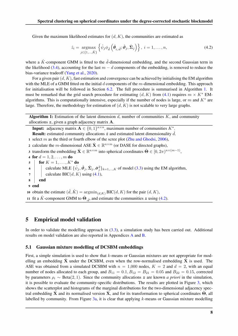
Algorithm 1: Estimation of the latent dimension d, number of communities K, and communityallocations z, given a graph adjacency matrix A.

Input: adjacency matrix A ∈ {0, 1}n×n, maximum number of communities K∗.Result: estimated community allocations z and estimated latent dimensionality d.

1 select m as the third or fourth elbow of the scree plot (Zhu and Ghodsi, 2006),2 calculate the m-dimensional ASE X ∈ Rn×m (or DASE for directed graphs),3 transform the embedding X ∈ Rn×m into spherical coordinates Θ ∈ [0, 2π)n×(m−1),4 for d = 1, 2, . . . ,m do5 for K = 1, . . . ,K∗ do6 calculate MLE {ψj , ϑj , Σj , σ

2j }k=1,...,K of model (3.3) using the EM algorithm,

7 calculate BIC(d,K) using (4.1),8 end9 end

10 obtain the estimate (d, K) = argmin(d,K) BIC(d,K) for the pair (d,K),11 fit a K-component GMM to Θ:d, and estimate the communities z using (4.2).

5 Empirical model validation

In order to validate the modelling approach in (3.3), a simulation study has been carried out. Additionalresults on model validation are also reported in Appendices A and B.

5.1 Gaussian mixture modelling of DCSBM embeddings

First, a simple simulation is used to show that k-means or Gaussian mixtures are not appropriate for mod-elling an embedding X under the DCSBM, even when the row-normalised embedding X is used. TheASE was obtained from a simulated DCSBM with n = 1,000 nodes, K = 2 and d = 2, with an equalnumber of nodes allocated to each group, and B11 = 0.1, B12 = B21 = 0.05 and B22 = 0.15, correctedby parameters ρi ∼ Beta(2, 1). Since the community allocations z are known a priori in the simulation,it is possible to evaluate the community-specific distributions. The results are plotted in Figure 3, whichshows the scatterplot and histograms of the marginal distributions for the two-dimensional adjacency spec-tral embedding X and its normalised version X, and for its transformation to spherical coordinates Θ, alllabelled by community. From Figure 3a, it is clear that applying k-means or Gaussian mixture modelling

8


(a) Scatterplot of xi

−1

0

1

X2

Community 1Community 2

−2 −1.5 −1 −0.5 0

X1

(b) Scatterplot of xi = xi/‖xi‖

−0.5

0

0.5

X2

Community 1Community 2

−1 −0.9 −0.8 −0.7 −0.6 −0.5

X1

(c) Histograms of θi = f2(xi)

0

0.5

1

1.5

3.8 4 4.2 4.4 4.6 4.8 5 5.2 5.4 5.6 5.8 6

0

1

2

3

Θ

Figure 3: Plots of xi, xi = xi/‖xi‖ and θi = f2(xi), obtained from the two dimensional ASE of a simulatedDCSBM. Joint (green) and community-specific (blue and red) marginal distributions with MLE Gaussianfit are also shown.

on X is suboptimal, since the joint distribution or cluster-specific marginal distributions are not normallydistributed, as predicted by the ASE-CLT (2.2). Figure 3b shows that row-normalisation is beneficial, sincethe marginal distributions for X2 are normally distributed within each community, but it is not appropriatefor modelling the joint distribution and for at least one of the two marginal distributions for X1. On the otherhand, the transformation Θ in Figure 3c visually meets the assumption of normality. This visual impressionis confirmed in Appendix A, which describes a CLT which strongly supports the normality in Θ for thetwo-dimensional case.

5.2 Structure of the likelihood

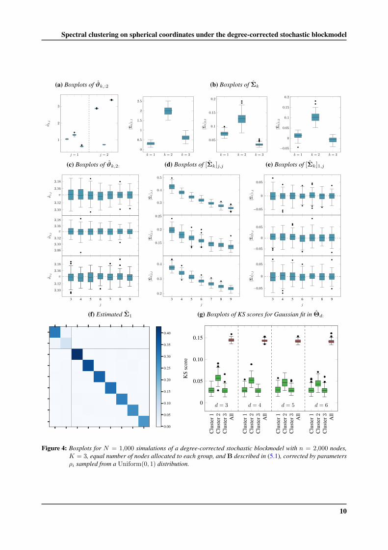
In order to validate the conjecture on the model likelihood proposed in (3.3), a simulation study has beencarried out. N = 1,000 DCSBMs with n = 2,000 nodes have been simulated, fixing K = 3, and pre-allocating the nodes to equal-sized clusters. The community-specific latent positions used in the simulationare µ1 = (0.7, 0.4, 0.1),µ2 = (0.1, 0.1, 0.5) and µ3 = (0.4, 0.8,−0.1), resulting in the block-probabilitymatrix:

B =

0.66 0.16 0.590.16 0.27 0.070.59 0.07 0.81

. (5.1)

The matrix is positive definite and has full rank 3, implying that d = 2 in the embedding Θ. For each ofthe N simulations, the link probabilities are corrected using the degree-correction parameters ρi sampledfrom a Uniform(0, 1) distribution, and the adjacency matrices A are obtained using (2.1). For each of thesimulated graphs ASE is calculated for a large value of m. The results are summarised in Figure 4.

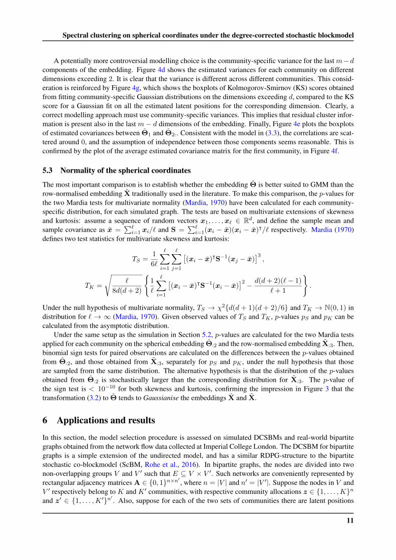
The true underlying cluster allocations are known in the simulation, and can be used to validate themodel assumptions. In this section, the community-specific mean and covariance matrices obtained fromthe embedding Θ of the sampled graph will be denoted as ϑk and Σk. Figure 4a shows the boxplots of thecommunity-specific estimated means for the first two components of Θ. The mean values show minimalvariation across the different simulations, and are clearly different from 0 and differ between clusters. InFigure 4b, boxplots for the community-specific estimated variances in Θ:d are plotted. Again, it seems thathaving cluster-specific variances is sensible, and at least one of the covariances is significantly different from0, as expected from the theory. On the other hand, Figure 4c shows the boxplots for the community-specificestimated means in Θd:, which are all centred at π. Hence, the assumption on the mean structure in (3.3)seems to be justified.

9


(a) Boxplots of ϑk,:2

j = 1 j = 2

1

2

3

ϑk,j

(b) Boxplots of Σk

k = 1 k = 2 k = 3

0

0.5

1

1.5

2

2.5

[Σk] 1,1

k = 1 k = 2 k = 3

0.05

0.1

0.15

0.2

[Σk] 2,2

k = 1 k = 2 k = 3

−0.05

0

0.05

0.1

0.15

0.2

[Σk] 1,2

(c) Boxplots of ϑk,2:

3.10

3.12

π

3.16

3.18

ϑ1,j

3.08

3.10

3.12

π

3.16

3.18

ϑ2,j

3 4 5 6 7 8 9

3.10

3.12

π

3.16

3.18

j

ϑ3,j

(d) Boxplots of [Σk]j,j

0.3

0.4

0.5

[Σ1] j,j

0.15

0.2

0.25

[Σ2] j,j

3 4 5 6 7 8 9

0.2

0.3

0.4

j

[Σ3] j,j

(e) Boxplots of [Σk]1,j

−0.05

0

0.05

[Σ1] 1,j

−0.05

0

0.05

[Σ2] 1,j

3 4 5 6 7 8 9

−0.05

0

0.05

j

[Σ3] 1,j

(f) Estimated Σ1

0.00

0.05

0.10

0.15

0.20

0.25

0.30

0.35

0.40

(g) Boxplots of KS scores for Gaussian fit in Θd:

Clu

ster

1C

lust

er2

Clu

ster

3A

ll

Clu

ster

1C

lust

er2

Clu

ster

3A

ll

Clu

ster

1C

lust

er2

Clu

ster

3A

ll

Clu

ster

1C

lust

er2

Clu

ster

3A

ll

0

0.05

0.10

0.15

d = 3 d = 4 d = 5 d = 6

KS

scor

e

Figure 4: Boxplots for N = 1,000 simulations of a degree-corrected stochastic blockmodel with n = 2,000 nodes,K = 3, equal number of nodes allocated to each group, and B described in (5.1), corrected by parametersρi sampled from a Uniform(0, 1) distribution.

10


A potentially more controversial modelling choice is the community-specific variance for the last m−dcomponents of the embedding. Figure 4d shows the estimated variances for each community on differentdimensions exceeding 2. It is clear that the variance is different across different communities. This consid-eration is reinforced by Figure 4g, which shows the boxplots of Kolmogorov-Smirnov (KS) scores obtainedfrom fitting community-specific Gaussian distributions on the dimensions exceeding d, compared to the KSscore for a Gaussian fit on all the estimated latent positions for the corresponding dimension. Clearly, acorrect modelling approach must use community-specific variances. This implies that residual cluster infor-mation is present also in the last m− d dimensions of the embedding. Finally, Figure 4e plots the boxplotsof estimated covariances between Θ1 and Θ2:. Consistent with the model in (3.3), the correlations are scat-tered around 0, and the assumption of independence between those components seems reasonable. This isconfirmed by the plot of the average estimated covariance matrix for the first community, in Figure 4f.

5.3 Normality of the spherical coordinates

The most important comparison is to establish whether the embedding Θ is better suited to GMM than therow-normalised embedding X traditionally used in the literature. To make this comparison, the p-values forthe two Mardia tests for multivariate normality (Mardia, 1970) have been calculated for each community-specific distribution, for each simulated graph. The tests are based on multivariate extensions of skewnessand kurtosis: assume a sequence of random vectors x1, . . . ,x` ∈ Rd, and define the sample mean andsample covariance as x =

∑`i=1 xi/` and S =

∑`i=1(xi − x)(xi − x)ᵀ/` respectively. Mardia (1970)

defines two test statistics for multivariate skewness and kurtosis:

TS =1

6`

∑i=1

∑j=1

[(xi − x)ᵀS−1(xj − x)

]3,

TK =

√`

8d(d+ 2)

{1

`

∑i=1

[(xi − x)ᵀS−1(xi − x)

]2 − d(d+ 2)(`− 1)

`+ 1

}.

Under the null hypothesis of multivariate normality, TS → χ2{d(d + 1)(d + 2)/6} and TK → N(0, 1) indistribution for ` → ∞ (Mardia, 1970). Given observed values of TS and TK , p-values pS and pK can becalculated from the asymptotic distribution.

Under the same setup as the simulation in Section 5.2, p-values are calculated for the two Mardia testsapplied for each community on the spherical embedding Θ:2 and the row-normalised embedding X:3. Then,binomial sign tests for paired observations are calculated on the differences between the p-values obtainedfrom Θ:2, and those obtained from X:3, separately for pS and pK , under the null hypothesis that thoseare sampled from the same distribution. The alternative hypothesis is that the distribution of the p-valuesobtained from Θ:2 is stochastically larger than the corresponding distribution for X:3. The p-value ofthe sign test is < 10−10 for both skewness and kurtosis, confirming the impression in Figure 3 that thetransformation (3.2) to Θ tends to Gaussianise the embeddings X and X.

6 Applications and results

In this section, the model selection procedure is assessed on simulated DCSBMs and real-world bipartitegraphs obtained from the network flow data collected at Imperial College London. The DCSBM for bipartitegraphs is a simple extension of the undirected model, and has a similar RDPG-structure to the bipartitestochastic co-blockmodel (ScBM, Rohe et al., 2016). In bipartite graphs, the nodes are divided into twonon-overlapping groups V and V ′ such that E ⊆ V × V ′. Such networks are conveniently represented byrectangular adjacency matrices A ∈ {0, 1}n×n′

, where n = |V | and n′ = |V ′|. Suppose the nodes in V andV ′ respectively belong to K and K ′ communities, with respective community allocations z ∈ {1, . . . ,K}nand z′ ∈ {1, . . . ,K ′}n′

. Also, suppose for each of the two sets of communities there are latent positions

11


(a) Undirected DCSBM

K = 2 K = 3

X X Θ X X Θ

Proportion of correct d 0.788 0.796 0.972 0.740 0.736 0.748Proportion of correct K 0.000 0.080 0.624 0.000 0.092 0.296

Average ARI 0.339 0.510 0.764 0.594 0.748 0.858

(b) Bipartite DCScBM

K = 2 K ′ = 3

X X Θ X′ X′ Θ′

Proportion of correct d 0.940 0.948 0.876 0.888 0.916 0.896Proportion of correct K 0.000 0.056 0.580 0.000 0.096 0.540

Average ARI 0.374 0.564 0.885 0.490 0.572 0.715

Table 1: Estimated performance for N = 250 simulated DCSBMs and bipartite DCScBMs.

µk ∈ Rd, k ∈ {1, . . . ,K}, and µ′` ∈ Rd, ` ∈ {1, . . . ,K ′}, such that µᵀkµ′` ∈ [0, 1]. This gives the link

probabilityAij ∼ Bernoulli(ρiρ

′jµ

ᵀziµ′z′j

), i ∈ V, j ∈ V ′, (6.1)

where ρi ∈ [0, 1] and ρ′j ∈ [0, 1] are degree correction parameters for each of the nodes in V and V ′.From A, it is possible to obtain embeddings X and X′ using the DASE in Section 2.2, and cluster the twoembeddings jointly or separately. In this work, the quality of the clustering is evaluated using the adjustedRand index (ARI, Hubert and Arabie, 1985). Higher values of the ARI correspond to better clusteringperformance, reaching a maximum of 1 for perfect agreement between the estimated clustering and the truelabels.

6.1 Synthetic networks

The performance of the model selection procedure described in Section 4 is evaluated on simulated DCS-BMs. N = 250 undirected graphs with n = 1,000 and K ∈ {2, 3} were simulated, randomly selecting Bfrom Uniform(0, 1)K×K and sampling the degree correction parameters from Beta(2, 1). The nodes wereallocated to communities of equal size. For each of the graphs, the models of Sanna Passino and Heard(2020) and Yang et al. (2020) are applied to the ASE X and its row-normalised version X for m = 10,selecting the estimates of d and K using BIC. The value m = 10 is usually approximately equal in thesimulations to the third elbow of the scree plot using the criterion of Zhu and Ghodsi (2006), considering atotal of 25 eigenvalues or singular values. Also, the model in (3.3) is fitted to Θ, estimating d and K usingthe selection procedure in Section 4, with K∗ = 6. The results of the simulations are reported in Table 1a.

A similar simulation has been repeated for bipartite DCScBMs. N = 250 graphs with n = 1,000 andn′ = 1,500 were generated, setting K = 2, K ′ = 3, communities of equal size, B ∼ Uniform(0, 1)K×K

′,

and ρi ∼ Beta(2, 1). The results are reported in Table 1b.The table shows that the transformed embedding sometimes has a slightly inferior performance when

estimating the correct value of the latent dimension d (cf. Table 1b), but outperforms the alternative method-ologies significantly in the ability to estimate the number of communities K. In particular, the Gaussianmixture model is not well suited to either the standard embedding X nor the row-normalised X, and thedistortion caused by the degree-corrections and row-normalisation does not allow correct estimation of K.This problem is alleviated when the spherical coordinates estimator is used. The improvement is reflected

12


(a) Proportion of correct dUndirected DCSBM

100 200 500 1000 20000

0.2

0.4

0.6

0.8

1

n

X

K = 2 X

K = 3 Θ

(b) Average ARIUndirected DCSBM

100 200 500 1000 20000

0.2

0.4

0.6

0.8

1

n

X

K = 2 X

K = 3 Θ

(c) Average ARIBipartite DCScBM

100 (150)200 (300)

500 (750)

1000 (1500)

2000 (3000)

0

0.2

0.4

0.6

0.8

1

+n (n′)

X (X′)K = 2 X (X′)K′ = 3 Θ (Θ′)

Figure 5: Estimated performance for N = 250 simulated DCSBMs and DCScBMs, for n ∈{100, 200, 500, 1000, 2000}. For bipartite DCScBMs, n′ ∈ {150, 300, 750, 1500, 3000}.

in a significant difference in the clustering performance, demonstrated by the average ARI scores for thethree different procedures. The table also shows that estimates of d based on the model of Sanna Passinoand Heard (2020) and Yang et al. (2020) on X and X′ seem to be slightly more accurate than alternativemethods on the DCScBM. It might be therefore tempting to construct a hybrid model that uses Θ:d forthe top-d embeddings and Xd: for the remaining components, and proceed to select the most appropriate dunder such a joint model. Unfortunately, model comparison via BIC is not possible in that setting.

The simulation is also repeated for different values of n, evaluating the asymptotic behaviour of theproposed community detection procedure. The results are plotted in Figure 5, demonstrating that the per-formance of the spherical coordinates estimator improves when the number of nodes in the graph increases.This appears to be consistent with the CLT presented in Appendix A. On the other hand, the results obtainedfrom the alternative estimators degrade with n, providing further evidence that the proposed model (3.3)appears to be more appropriate for community detection under the DCSBM.

Also, the boxplots for the paired differences between ARIs are plotted in Figure 6. The clusteringbased on Θ consistently outperforms X and X (cf. Figure 6a and 6c). The difference can be quantitativelyevaluated using binomial sign tests for paired observations, similarly to Section 5.3. For both undirected andbipartite graphs, the p-values of the sign tests are < 10−10, overwhelmingly suggesting that the clusteringbased on Θ is superior to the competing methodologies. Furthermore, the difference increases when thenumber of nodes increases (cf. Figure 6b). Overall, the simulations suggest that the proposed spectralclustering procedure for estimation of the DCSBM, based on the spherical coordinates of the ASE estimatorof the latent positions, appears to outperform competing estimators, including spectral clustering on therow-normalised ASE estimator.

6.2 Imperial College network flow data

The model proposed in this work has been specifically developed for clustering networks obtained fromthe network flow data collected at Imperial College London (ICL). Finding communities of machines withsimilar behaviour is important in network monitoring and intrusion detection (Neil et al., 2013). In thisapplication, the edges relate to all the HTTP (port 80) and HTTPS (port 443) connections observed frommachines hosted in computer labs in different departments at ICL in January 2020. The source nodes Vare computers hosted in college laboratories, and the destination nodes V ′ are internet servers. Intuitively,computers in a laboratory tend to have a heterogeneous degree distribution of their web connections becausethey are not used uniformly: a computer located closed to the entrance of the laboratory might be used more

13


(a) Undirected graphK ∈ {2, 3}, n = 1000

−0.5 0 0.5

Θ vs. XK = 3

Θ vs. XK = 3

Θ vs. XK = 2

Θ vs. XK = 2

Paired differences in ARI

(b) Undirected graph, K = 2Varying n, Θ vs. X

−1 −0.5 0 0.5

2000

1000

500

200

100


n

(c) Bipartite graph, K = 2, K ′ = 3,n = 1000, n′ = 1500

−0.5 0 0.5

Θ′ vs. X′

Θ′ vs. X′

Θ vs. X

Θ vs. X


Figure 6: Boxplots of differences in ARI for N = 250 simulated DCSBMs and DCScBM.

Name |V | |V ′| |E| K ZG3 ZG4

ICL1 628 54,111 668,155 3 24 52ICL2 439 60,635 717,912 4 24 53ICL3 1,011 84,664 1,470,074 5 27 51

Table 2: Summary statistics for the Imperial College London computer networks.

than a machine at the back. Therefore, the total time of activity is different across machines in the samecommunity, which suggests that the DCSBM is an appropriate modelling choice. This is confirmed by thewithin-community degree distributions in Figure 1 (Section 1), which compares one of the Imperial Collegenetworks (ICL2, cf. Figure 1c) with a simulated SBM and DCSBM (cf. Figures 1a and 1b)1.

Three real-world computer networks are considered here, and corresponding summary statistics are pre-sented in Table 2, where ZG` denotes the position of the `-th elbow of the scree plot according to the methodof Zhu and Ghodsi (2006). For the source nodes, a known underlying community structure is given by thedepartment to which each machine belongs. ICL1 corresponds to machines hosted in the departments ofPhysics, Electrical Engineering, and Earth Science, whereas computers in Chemistry, Civil Engineering,Mathematics, and Medicine are considered in ICL2. For ICL3, the departments are Aeronautical Engi-neering, Civil Engineering, Electrical Engineering, Mathematics, and Physics. Students use the computerlaboratories for tutorials and classes, and therefore some variation might be expected in the activities ofdifferent machines across different departments.

Figure 7 shows the scatterplots of the leading 2 dimensions of them-dimensional embeddings X, X andΘ for m = 30 for ICL2, showing that the clustering task is particularly difficult in this network, and thereis not much separation between the communities. Despite this, the transformation to spherical coordinates(cf. Figure 7c) appears to make the communities more Gaussian-shaped, as opposed to the standard androw-normalised DASE, where the within-community embeddings are curved (cf. Figure 7a and 7b), andtherefore not amenable to Gaussian mixture modelling. This impression is quantitatively confirmed by theMardia tests for multivariate normality on each community (cf. Section 5.3): the difference of the log-p-values obtained from the spherical coordinates transformation and the standard DASE is on average ≈ 42for the kurtosis and ≈ 82 for the skewness, further demonstrating that the proposed transformation tends toGaussianise the embedding.

1Figure 1a displays the within-community out-degree distribution of a simulated ScBM, see (6.1), with K = K′ = 4, equal-sized communities, and block-community matrix B/2 (see below). Figure 1b displays the same distribution for a simulatedDCScBM with block-community matrix 2B, corrected sampling ρi, ρ′j ∼ Beta(3, 5). For B: B11 = 0.35, B22 = 0.25,B33 = 0.15, B44 = 0.1, Bk` = 0.1 if k 6= `.

14


(a) X:2

−2 −1.5 −1 −0.5 0−1.5

−1

−0.5

0

0.5

1

1.5

2

X1

X2

ChemistryCivil EngineeringMathematicsMedicine

(b) X:2

−0.7 −0.6 −0.5 −0.4 −0.3 −0.2−0.8

−0.6

−0.4

−0.2

0

0.2

0.4

X1X

2

(c) Θ:2

3.5 4 4.5 5 5.5

1.5

2

2.5

3

3.5

4

4.5

5

Θ1

Θ2

Figure 7: ICL2: scatterplot of the leading two dimensions for X, X and Θ.

(a) Estimated (d,K)

m = 30 m = 50

X X Θ X X Θ

ICL1 (26, 6) (11, 6) (11, 4) (22, 5) (11, 6) (11, 4)ICL2 (28, 5) (8, 7) (15, 4) (29, 4) (8, 7) (15, 4)ICL3 (24, 10) (17, 5) (15, 5) (25, 6) (13, 6) (16, 5)

(b) ARIs for the estimated clustering

m = 30 m = 50 Alternative methods

X X Θ X X Θ Louvain Paris HLouvain

ICL1 0.259 0.324 0.418 0.262 0.317 0.418 0.107 0.082 0.152ICL2 0.441 0.736 0.938 0.359 0.743 0.938 0.488 0.560 0.602ICL3 0.246 0.342 0.409 0.269 0.265 0.364 0.079 0.032 0.157

Table 3: Estimates of (d,K) and ARIs for the embeddings X, X and Θ for m ∈ {30, 50} and alternative methodolo-gies.

For each of the three ICL network graphs, the DASE has been calculated for m = 30 and m = 50,and the model in Sanna Passino and Heard (2020) and Yang et al. (2020) has been fitted on the sourceembeddings X and the row-normalised version X, whereas the model (3.3) is used on the transformationΘ, setting K∗ = 20. The resulting estimated values of d and K, obtained using the minimum BIC, arereported in Table 3a. In order to reduce the sensitivity to initialisation, the model was fitted 10 times foreach pair (d,K), and the parameter estimates corresponding to the minimum BIC were retained. The choiceofm ∈ {30, 50} corresponds to values around the third and fourth elbows in the scree plot of singular values,according to the criterion of Zhu and Ghodsi (2006) (cf. Table 2).

Comparing Table 3a for the two different values of m, it seems that the estimates of K based on Θ arecloser to the underlying true number of communities. In particular, K = 3 for ICL1, K = 4 for ICL2, andK = 5 for ICL3, based on the number of departments.

Based on the estimates in Table 3a, the estimated community allocations zi were obtained using (4.2),and the adjusted Rand index was calculated using the department as labels. For further comparisons, the re-sults were compared to other popular community detection methods: the Louvain algorithm (Blondel et al.,2008) adjusted for bipartite graphs (Dugué and Perez, 2015), and the hierarchical Louvain (HLouvain) and

15


Paris methods (Bonald et al., 2018), all in their default implementation for bipartite graphs in the pythonlibrary scikit-network. The results are reported in Table 3b. Clearly, clustering on the embedding Θ out-performs the alternatives, including X and X, in all the three networks. In some cases, the improvement issubstantial, for example in ICL2, where the proposed method reaches the score 0.938, corresponding to only9 misclassified nodes out of 439, particularly remarkable considering the lack of separation of the clustersin Figure 7.

The results were confirmed by binomial paired sign tests on the difference between ARI scores forN = 25 iterations of the community detection algorithms, which returned p-values < 10−4 in favour of thespherical coordinates estimator over the alternative methodologies.

In terms of network structure, the results could be interpreted as follows: the computers connect to a setof shared college-wide web servers (for example, the virtual learning environment and the library services),and to services specific to the discipline carried out in each department. Furthermore, each machine hasdifferent levels of activity, which leads to heterogeneous within-community degree distributions. The SBM,corresponding to X, only clusters the nodes based on their degree, whereas the DCSBM is able to uncoverthe departmental structure, in particular when the spherical coordinates estimator Θ is used. Under theassumption that the networks were generated under a DCSBM, the results confirm that the estimate basedon spherical coordinates proposed in this work appears to produce superior results when compared to thestandard or row-normalised ASE.

7 Conclusion

In this article, a novel method for spectral clustering under the degree-corrected stochastic blockmodel hasbeen proposed. The model is based on a transformation to spherical coordinates of the commonly usedadjacency spectral embedding. Such a transformation seems more suited to Gaussian mixture modellingthan the row-normalised embedding, which is widely used in the literature for spectral clustering. Theproposed methodology is then incorporated within a simultaneous model selection scheme that allows themodel dimension d and the number of communities K to be determined. The optimal values of d and Kare chosen using the popular Bayesian information criterion. The framework also extends simply to includedirected and bipartite graphs. Results on synthetic data and real-world computer networks show superiorperformance over competing methods.

ReferencesAlanis-Lobato, G., Mier, P. and Andrade-Navarro, M. A. (2016) Efficient embedding of complex networks to hyper-

bolic space via their Laplacian. Scientific Reports, 6, 30108.

Amini, A. A., Chen, A., Bickel, P. J. and Levina, E. (2013) Pseudo-likelihood methods for community detection inlarge sparse networks. Annals of Statistics, 41, 2097–2122.

Athreya, A., Priebe, C. E., Tang, M., Lyzinski, V., Marchette, D. J. and Sussman, D. L. (2016) A limit theorem forscaled eigenvectors of random dot product graphs. Sankhya A, 78, 1–18.

Blondel, V. D., Guillaume, J.-L., Lambiotte, R. and Lefebvre, E. (2008) Fast unfolding of communities in largenetworks. Journal of Statistical Mechanics: Theory and Experiment, P10008.

Bonald, T., Charpentier, B., Galland, A. and Hollocou, A. (2018) Hierarchical graph clustering based on node pairsampling. In Proceedings of the 14th International Workshop on Mining and Learning with Graphs (MLG).

Braun, M. and Bonfrer, A. (2011) Scalable inference of customer similarities from interactions data using Dirichletprocesses. Marketing science, 30, 513–531.

Chaudhuri, K., Chung, F. and Tsiatas, A. (2012) Spectral clustering of graphs with general degrees in the extendedplanted partition model. In Proceedings of the 25th Annual Conference on Learning Theory, vol. 23.

16


Chen, Y., Li, X. and Xu, J. (2018) Convexified modularity maximization for degree-corrected stochastic block models.Annals of Statistics, 46, 1573–1602.

Dempster, A., Laird, N. and Rubin, D. (1977) Maximum likelihood from incomplete data via the EM algorithm.Journal of the Royal Statistical Society, Series B, 39, 1–38.

Dugué, N. and Perez, A. (2015) Directed Louvain: maximizing modularity in directed networks. Tech. Rep. hal-01231784, Université d’Orléans.

Fraley, C. and Raftery, A. E. (2002) Model-based clustering, discriminant analysis, and density estimation. Journal ofthe American Statistical Association, 97, 611–631.

Gao, C., Ma, Z., Zhang, A. Y. and Zhou, H. H. (2018) Community detection in degree-corrected block models. Annalsof Statistics, 46, 2153–2185.

Gulikers, L., Lelarge, M. and Massoulié, L. (2017) A spectral method for community detection in moderately sparsedegree-corrected stochastic block models. Advances in Applied Probability, 49, 686–721.

Holland, P. W., Laskey, K. B. and Leinhardt, S. (1983) Stochastic blockmodels: First steps. Social Networks, 5,109–137.

Hubert, L. and Arabie, P. (1985) Comparing partitions. Journal of Classification, 2, 193–218.

Jin, J. (2015) Fast community detection by SCORE. Annals of Statistics, 43, 57–89.

Jones, A. and Rubin-Delanchy, P. (2020) The multilayer random dot product graph. arXiv e-prints.

Karrer, B. and Newman, M. E. J. (2011) Stochastic blockmodels and community structure in networks. PhysicalReview E, 83.

Krioukov, D., Papadopoulos, F., Kitsak, M., Vahdat, A. and Boguñá, M. (2010) Hyperbolic geometry of complexnetworks. Physical Review E, 82.

Lei, J. and Rinaldo, A. (2015) Consistency of spectral clustering in stochastic block models. Annals of Statistics, 43,215–237.

von Luxburg, U. (2007) A tutorial on spectral clustering. Statistics and Computing, 17.

Mardia, K. V. (1970) Measures of multivariate skewness and kurtosis with applications. Biometrika, 57, 519–530.

McCormick, T. H. and Zheng, T. (2015) Latent surface models for networks using aggregated relational data. Journalof the American Statistical Association, 110, 1684–1695.

Meyer, C. D. (2000) Matrix analysis and applied linear algebra. SIAM.

Neil, J., Hash, C., Brugh, A., Fisk, M. and Storlie, C. B. (2013) Scan statistics for the online detection of locallyanomalous subgraphs. Technometrics, 55, 403–414.

Ng, A. Y., Jordan, M. I. and Weiss, Y. (2001) On spectral clustering: Analysis and an algorithm. In Proceedings of the14th International Conference on Neural Information Processing Systems: Natural and Synthetic, 849–856.

Peng, L. and Carvalho, L. (2016) Bayesian degree-corrected stochastic blockmodels for community detection. Elec-tronic Journal of Statistics, 10, 2746–2779.

Qin, T. and Rohe, K. (2013) Regularized spectral clustering under the degree-corrected stochastic blockmodel. InProceedings of the 26th International Conference on Neural Information Processing Systems, vol. 2, 3120–3128.

Raftery, A. E. and Dean, N. (2006) Variable selection for model-based clustering. Journal of the American StatisticalAssociation, 101, 168–178.

Rohe, K., Qin, T. and Yu, B. (2016) Co-clustering directed graphs to discover asymmetries and directional communi-ties. Proceedings of the National Academy of Sciences.

17


Rubin-Delanchy, P., Cape, J., Tang, M. and Priebe, C. E. (2017) A statistical interpretation of spectral embedding: thegeneralised random dot product graph. arXiv e-prints.

Sanna Passino, F. and Heard, N. A. (2020) Bayesian estimation of the latent dimension and communities in stochasticblockmodels. Statistics and Computing, 30, 1291–1307.

Sussman, D. L., Tang, M. and Priebe, C. E. (2014) Consistent latent position estimation and vertex classification forrandom dot product graphs. IEEE Transactions on Pattern Analysis and Machine Intelligence, 36, 48–57.

Tang, M. and Priebe, C. E. (2018) Limit theorems for eigenvectors of the normalized Laplacian for random graphs.Annals of Statistics, 46, 2360–2415.

Yang, C., Priebe, C. E., Park, Y. and Marchette, D. J. (2020) Simultaneous dimensionality and complexity modelselection for spectral graph clustering. Journal of Computational and Graphical Statistics, 30, 422–441.

Young, S. J. and Scheinerman, E. R. (2007) Random dot product graph models for social networks. In Algorithms andModels for the Web-Graph, 138–149.

Zhao, Y., Levina, E. and Zhu, J. (2012) Consistency of community detection in networks under degree-correctedstochastic block models. Annals of Statistics, 40, 2266–2292.

Zhu, M. and Ghodsi, A. (2006) Automatic dimensionality selection from the scree plot via the use of profile likelihood.Computational Statistics & Data Analysis, 51, 918 – 930.

A A central limit theorem on spherical coordinates

In this section, it is demonstrated that, for d = 2, the spherical coordinates obtained from ASE asymptoti-cally converge to the spherical coordinates of the true underlying latent positions, with Gaussian error. Thisproperty is particularly important, since points belonging to the same community share the same sphericalcoordinates under the DCSBM.

Consider the covariance Σk(ρ) appearing in the ASE-CLT (2.2), which holds under the assumptionof d fixed and known. The covariance matrix Σk(ρ) can be calculated explicitly, and arises as a corol-lary of the ASE-CLT, taking the RDPG inner product distribution to be the product measure F = Gρ ⊗∑K

k=1 ψkδµk,∑K

k=1 ψk = 1, ψk ≥ 0,whereGρ is the distribution of the degree-correction parameters, andδ· is the Dirac’s delta measure. Letting ξ ∼ F be a d-dimensional random vector, the k-th community covari-ance matrix then takes the form Σk(ρ) = ∆−1E{ρµᵀ

kξ(1− ρµᵀkξ)ξξᵀ}∆−1, where ∆ = E(ξξᵀ) ∈ Rd×d

is the second moment matrix, assumed to be invertible.The ASE-CLT (2.2) provides the theoretical framework for establishing a central limit theorem for the

spherical coordinates estimator under the DCSBM for d = 2. Let θ = f2(x) be the spherical coordinatesfor the true latent position x ∈ R2, and θ(n) = f2(x

(n)) be the corresponding estimator calculated fromx(n) ∈ R2. Note that for d = 2, Q(n) ∈ O(2), the orthogonal group in two dimensions, which consists inrotation and reflection matrices:

Qrot(ϕ) =

[cos(ϕ) sin(ϕ)− sin(ϕ) cos(ϕ)

], Qref(ϕ) =

[− cos(ϕ) sin(ϕ)sin(ϕ) cos(ϕ)

].

The rotation matrix Qrot(ϕ) applied to x ∈ R2 rotates the vector by an angle ϕ (taken clockwise) withrespect to the second axis, whereas a reflection matrix Qref(ϕ) reflects the vector with respect to a linepassing through the origin, with angle ϕ/2 (taken clockwise) to the second axis. It follows that any matrixQ(n) ∈ O(2) appearing in the ASE-CLT (2.2) is uniquely mapped to an angle ϕ(n) ∈ [−2π, 2π) such that:

f2(Q(n)x(n)) = (f2(x

(n)) + ϕ(n)) mod 2π = (θ(n) + ϕ(n)) mod 2π.

18


(a) Boxplots of ϑk,2

3

π

3.4

ϑ1,2

3

π

3.4

ϑ2,2

100 200 500 1000 2000

3

π

3.4

n

ϑ3,2

(b) Boxplots of [Σk]1,3

−0.5

0

0.5

[Σ1] 1,3

−1

0

1

[Σ2] 1,3

100 200 500 1000 2000

−0.5

0

0.5

n

[Σ3] 1,3

(c) Boxplots of [Σk]3,4

−0.4

−0.2

0

0.2

[Σ1] 3,4

−0.5

0

0.5

[Σ2] 3,4

100 200 500 1000 2000

−0.2

0

0.2

n

[Σ3] 3,4

Figure 8: Boxplots for N = 1,000 simulations of a degree-corrected stochastic blockmodel with varying number ofnodes n, K = 3, equal number of nodes allocated to each group, and B described in (5.1), corrected byparameters ρi sampled from a Uniform(0, 1) distribution.

The ASE-CLT (2.2) can be extended to spherical coordinates by the multivariate delta method, with trans-formation function f2(·), see (3.2). The multivariate delta method establishes that, conditional on the com-munity allocation, correction parameter and orthogonal matrices Q(n) ∈ O(2), the spherical coordinates areasymptotically Gaussian:

limn→∞

P{√

n(θ(n) − θ − ϕ(n)

)≤ v

∣∣∣ z = k, ρ}→ Φ1 {v,∇x(θ)ᵀΣk(ρ)∇x(θ)} ,

where v ∈ R, and ∇x(θ) is the gradient of θ with respect to x, under the assumption that (θ(n)+ϕ(n)) mod2π = θ(n) + ϕ(n). The gradient is:

∇x(θ) =

(∂θ

∂x1,∂θ

∂x2

)ᵀ

=

(0,−2 · sign(x1)

√1− x22/‖x‖2

/‖x‖

)ᵀ

.

B Empirical model validation: additional simulations

B.1 Asymptotic behaviour

The proposed model is further validated by a study with increasing values for the number of nodes n.N = 1,000 graphs are simulated using the same configuration as the simulation in Figure 4, for n ∈{100, 200, 500, 1000, 2000}. Figure 8 reports the boxplots for the different values of n for three of theestimated parameters, suggesting that the asymptotic behaviour of the embedding is consistent with themodelling choices in (3.3). In particular, three assumptions are checked: means centred at π in the lastm − d components (cf. Figure 8a), independence between the initial d and last m − d components (cf.Figure 8b), and independence within the last m− d components (cf. Figure 8c).

B.2 Changes in the correlation between blocks

The same model assumptions are also checked with different values of the correlation between blocks.N = 100 graphs with K = 2 equal-sized communities and n = 500 nodes are simulated from a DCSBM

19


with B11 = 0.5, B22 = 0.35 and B12 = B21 = r, r ∈ {0.05, 0.1, 0.15, 0.2, 0.25, 0.3, 0.35}, corrected byρi ∼ Uniform(0, 1). The results plotted in Figure 9 suggest that the assumptions in model (3.3) are robustto changes in the correlation between the blocks.

(a) Boxplots of ϑk,2

3

3.1

π

3.2

3.3

ϑ1,2

0.05 0.1 0.15 0.2 0.25 0.3

3

3.1

π

3.2

r

ϑ2,2

(b) Boxplots of [Σk]1,3

−0.1

0

0.1

[Σ1] 1,3

0.05 0.1 0.15 0.2 0.25 0.3

−0.1

0

0.1

r

[Σ2] 1,3

(c) Boxplots of [Σk]3,4

−0.1

0

0.1

[Σ1] 3,4

0.05 0.1 0.15 0.2 0.25 0.3

−0.1

0

0.1

r

[Σ2] 3,4

Figure 9: Boxplots for N = 100 simulations of a degree-corrected stochastic blockmodel with n = 500, K = 2,equal number of nodes allocated to each group, B11 = 0.5, B22 = 0.35 and B12 = B21 = r, for differentvalues of r, corrected by parameters ρi sampled from a Uniform(0, 1) distribution.

20

spectral clustering on spherical coordinates under the

Documents