Spectral analysis for point processes. Error bars.

Bijan Pesaran

Center for Neural Science

New York University

Overview

Spectral analysis for point processes

Estimating error bars for spectral quantities

Spectral analysis for point processes

Analyzing point processes

Conditional intensity Probability of finding a point conditioned on past

history Specifying the moments of functions

Correlation functions and spectra

Point process representations Counting process

Interval process

ii

dN tt t

dt i

i

dN tt t

dt

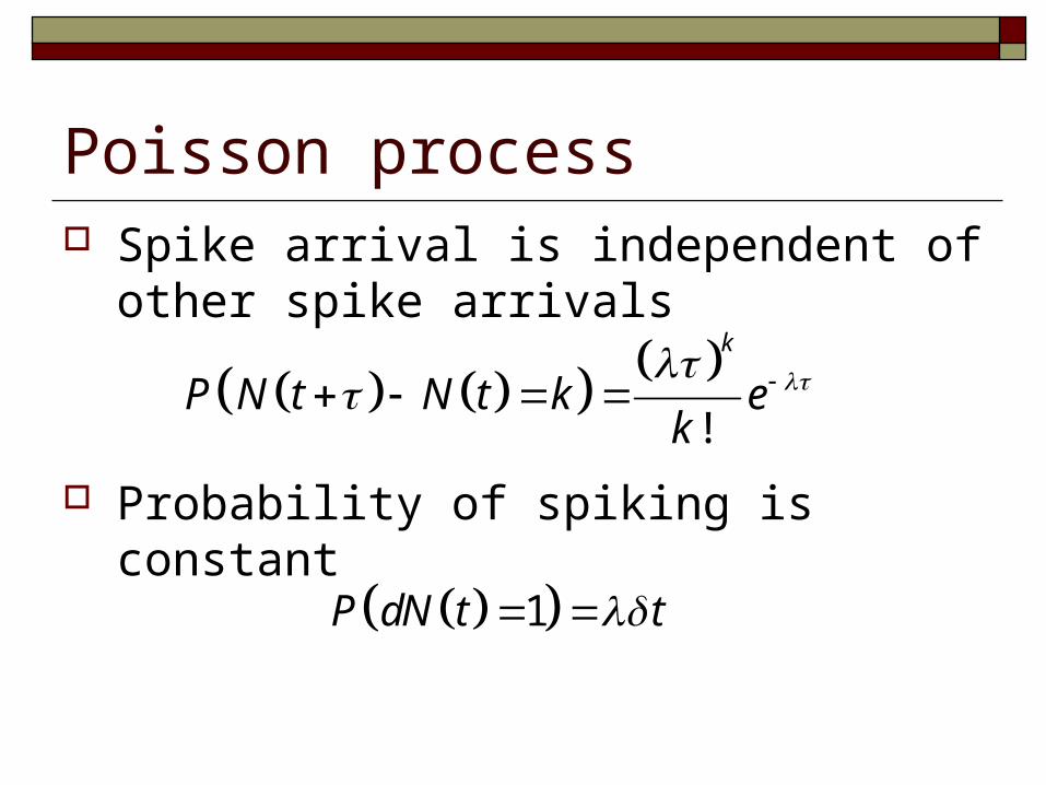
Poisson process Spike arrival is independent of other spike

arrivals

Probability of spiking is constant

!

k

P N t N t k ek

1P dN t t

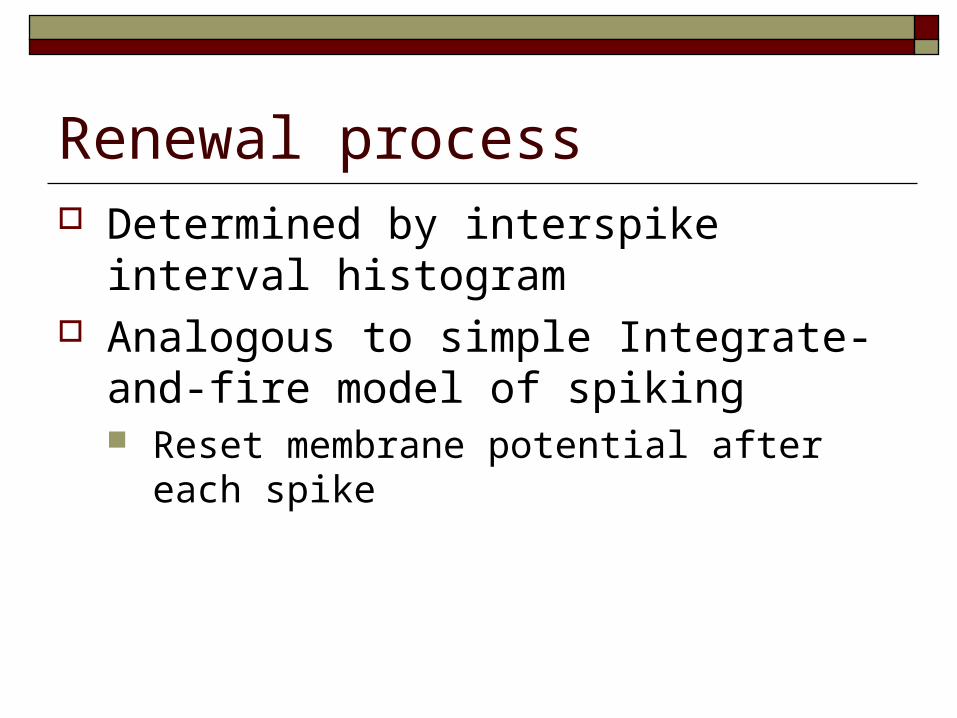
Renewal process Determined by interspike interval histogram Analogous to simple Integrate-and-fire model

of spiking Reset membrane potential after each spike

Conditional intensity process Probability of occurrence of a point at a given

time, given the past history of the process

This is a stochastic process that depends on the specific realization. It is not a rate-varying Poisson process

1 2| , ,..., ;nt t t t n

Probability of spike in t,t+dt

Methods of moments Specify process in terms of the moments of

the process i

i

dN tt t

dt

E dN t

dt

1 2

1 2

E dN t dN t

dt dt

First moment:

Second moment:

Second moment of point process Correlation function

1 2 1 2 1 2 1 2C t t dt dt E dN t dN t E dN t E dN t

Spectrum of point process Spectrum is the Fourier transform of the

correlation function

2 ifS f C e d

limfS f

0limT

V N TSF

S E N T

High-frequency limit:

Low-frequency limit:

Number covariation Low-frequency limit of the coherence is the

number covariation

0

cov ,lim

i j

ijf

i j

N NC f

V N V N

Illustrative point process spectra

Poisson Periodic Refractory

Features of spike spectrum Dip at low frequency due to refractoriness

Rate-varying Poisson process

2

22

1exp

22C

2 2 2exp 2S f f

S f S f

Example spike spectrum

Not Poisson process

Not rate-varying Poisson process

Spike correlation and spectrumAuto-correlation fn Multitaper spectrum

NT = 8

Spike cross-correlation and coherenceCross-correlation fn Multitaper coherence

9 trials, NT=9

Example correlation - coherence

Error bars

Asymptotic distribution of DFT Let be a Gaussian process

is Gaussian since it is a sum of Gaussian variables

has a distribution with chi-squared form with two degrees of freedom, since is complex.

is distributed independently of T Therefore, variance does not decrease as T

increases - the estimator is inconsistent This is true for non-Gaussian if is the

sum of many data points, from the CLT.

x t

TX f

TX f 2

TX f

2

TX f

x t TX f

Degrees of freedom Variance of is equal to square of mean

because it has 2 degrees of freedom

Multitaper estimates have more degrees of freedom

2

TX f

22

22

T

E X fVar X f

2 trv KN

2ˆ ~S f

S f

Finite size effects for point process spectrum (Jarvis and Mitra 2001) Number of spikes affects degrees of freedom

of point process spectral estimates

For tapering to help, need at least as many spikes per trial as tapers

22 2 2 1

Ttr

Var X f E X fN T

1 1 1

2eff trN T 2eff tr

NKN

N K

N is average number ofspikes in each trial

Distribution of coherence Under null hypothesis that there is no

coherence, coherence is distributed:

Coherence will exceed the value below with probability p

2 222 1P C C C

1 2 11 p

Rule of thumb for coherence According to analytic distribution

50 trials, 5 tapers, p=0.05, C > 0.11 50 trials, 19 tapers, p=0.05, C > 0.056

Rule of thumb: Variance of coherence is 2/DOF.

50 trials, 5 tapers, p=0.05, C>0.13 50 trials, 19 tapers, p=0.05, C>0.065

1.96

tr

CN K

Finite size effects for coherence Degrees of freedom for spike-spike coherence

and spike-field coherence are given by process with smallest number of degrees of freedom.

Phase of coherence Defined as

Gaussian distributed – 95% confidence interval:

2

2 1ˆ 2 1fC f

1ˆ tan Im Ref C C

Brillinger 1974

Rosenberg et al 1989

Variance-stabilizing transformations Spectrum: Logarithm

Variance constant and not equal to mean Coherence: Arc-tanh

Transforms 0-1 to real line. Coherence

Phase of the coherence

Jackknife Basic idea: Given sequence of observations

and a statistic

Define pseudovalues

Then, Jackknife estimate of is

1 2, , , nx x x 1 2, , , nx x x

1 1 1 1, , 1 , , , , ,in i i nn x x n x x x x

1

1 ni

JKin

Jackknife The jackknife estimate of the variance of is

It can be shown that

Approximately follows a t-distribution with n-1 degrees of freedom.

2

2

1

1

1

ni

JK JKin n

JK

JK

Jackknife The Jackknife can be applied to spectral

estimates by leaving one trial-taper combination in turn. Typically applied to the variance stabilized spectral and coherences

1 1ˆ ˆˆ ˆexp 1 exp 12 2m mS f t S S f t

Other resampling methods Resample to determine the empirical

distribution.

Estimate variance and use Normal approximation

Determine Percentile intervals Need a LOT of samples to estimate the tails of the

empirical distribution ~10,000

LFP spectrogram error barsMultitaper estimate

- 95% Chi2Multitaper estimate

- 95% Jackknife

Spike coherence error barsMultitaper coherence

9 trials, NT=12Multitaper coherence

9 trials, NT=8

Summary Spectral analysis can be used to understand

both continuous and point processes

Sensitive test to discriminate models of spike trains

Error bars can be constructed for all spectral quantities using standard procedures